Retrieving Secondary Forest Aboveground Biomass from Polarimetric ALOS-2 PALSAR-2 Data in the Brazilian Amazon

Abstract

Secondary forests (SF) are important carbon sinks, removing CO₂ from the atmosphere through the photosynthesis process and storing photosynthates in their aboveground live biomass (AGB). This process occurring at large-scales partially counteracts C emissions from land-use change, playing, hence, an important role in the global carbon cycle. The absorption rates of carbon in these forests depend on forest physiology, controlled by environmental and climatic conditions, as well as on the past land use, which is rarely considered for retrieving AGB from remotely sensed data. In this context, the main goal of this study is to evaluate the potential of polarimetric (quad-pol) ALOS-2 PALSAR-2 data for estimating AGB in a SF area. Land-use was assessed through Landsat time-series to extract the SF age, period of active land-use (PALU), and frequency of clear cuts (FC) to randomly select the SF plots. A chronosequence of 42 SF plots ranging 3–28 years (20 ha) near the Tapajós National Forest in Pará state was surveyed to quantifying AGB growth. The quad-pol data was explored by testing two regression methods, including non-linear (NL) and multiple linear regression models (MLR). We also evaluated the influence of the past land-use in the retrieving AGB through correlation analysis. The results showed that the biophysical variables were positively correlated with the volumetric scattering, meaning that SF areas presented greater volumetric scattering contribution with increasing forest age. Mean diameter, mean tree height, basal area, species density, and AGB were significant and had the highest Pearson coefficients with the Cloude decomposition (λ3), which in turn, refers to the volumetric contribution backscattering from cross-polarization (HV) (ρ = 0.57–0.66, p-value < 0.001). On the other hand, the historical use (PALU and FC) showed the highest correlation with angular decompositions, being the Touzi target phase angle the highest correlation (Φs) (ρ = 0.37 and ρ = 0.38, respectively). The combination of multiple prediction variables with MLR improved the AGB estimation by 70% comparing to the NL model (R² adj. = 0.51; RMSE = 38.7 Mg ha⁻¹) bias = 2.1 ± 37.9 Mg ha⁻¹ by incorporate the angular decompositions, related to historical use, and the contribution volumetric scattering, related to forest structure, in the model. The MLR uses six variables, whose selected polarimetric attributes were strongly related with different structural parameters such as the mean forest diameter, basal area, and the mean forest tree height, and not with the AGB as was expected. The uncertainty was estimated to be 18.6% considered all methodological steps of the MLR model. This approach helped us to better understand the relationship between parameters derived from SAR data and the forest structure and its relation to the growth of the secondary forest after deforestation events.

1. Introduction

Secondary forests (SFs) are defined as areas of forests where clear cut was made only by anthropic actions, whether or not for conversion to other land uses, according to the Convention on Biological Diversity (CDB) [1]. Despite the multiple definitions of SFs found in the literature [2,3,4,5], hereafter, we consider as SFs areas that are in a process of regeneration after complete removal of primary forests (PFs) through clear cut or areas with characteristics in conformity with the definition proposed by the CDB [1]. This definition was chosen because it adequately encompasses the classes of SF discriminated by satellite data on a regional or global scale [6].

According to Forest Resources Assessment FRA/FAO [7], from 106 nations located in the tropics, 36 have all remaining forests composed of SFs, almost half of all tropical countries have the majority of their forest land dominated by SFs, and only 19 of them have the dominance of PF in their territory, including Brazil. These numbers have led some authors to recognize the importance of SFs, not only because of the capacity of these forests in maintaining biodiversity and mitigating anthropogenic carbon emissions, but also because SFs are likely to be the dominant state of rainforests in the future [2,8,9,10,11,12].

Forests undergoing regeneration partially offset carbon emissions from land use change and fossil fuels by accumulating carbon in their biomass. It has been estimated that SFs have the potential to accumulate 0.86 Pg C year⁻¹ in Latin America [10]. This value is twice as large as carbon emissions from land-use, land-use change, and forestry (LULUCF), which accounts for 0.47 Pg C year⁻¹ [13]. In the Brazilian Amazon, estimates of C accumulation in SFs vary between 0.06 Pg C year⁻¹ and 0.15 Pg C year⁻¹ [14,15]. Despite large uncertainties in these estimates, carbon uptake by SFs is likely to represent 17–44% of total carbon emission from deforestation in the Brazilian Amazon. To improve these estimates, it is therefore crucial to accurately quantify the extent and growth rates of SFs in the Amazonia [10,13,15,16]. For instance, the mean annual increment (MAI) of the aboveground biomass (AGB) varies from 0.16 Mg ha⁻¹ year⁻¹ to 30 Mg ha⁻¹ year⁻¹ throughout the Brazilian Amazon, with higher growth rates in the central Amazon (dry season < 4 months 100 mm rainfall) than in the eastern Amazon (dry season ≥ 4 months) regardless of the previous land-use [17,18,19,20,21]. Furthermore, the intensity of the previous land-use reduces about 35% of the MAI (7.45 Mg ha⁻¹ year⁻¹) in areas subjected to pasture and agricultural practices and about 40% (8.05 Mg ha⁻¹ year⁻¹) if the frequency of clear cuts are greater than twice, when compared to SFs areas with previous “light” land use [18,19,22,23,24,25,26].

Secondary forests covered between 140,000 km² and 228,000 km² until 2010 in the Brazilian Amazon [27,28,29], representing approximately 30% of accumulated deforestation since 1988 (PRODES/INPE) [30]. The estimation of the extent of the SF is often made using data from optical sensors [31,32]. However, the low ability of these sensors in separating succession classes, confusion with other vegetation classes, and the persistence of rain clouds may reduce the accuracy of these estimates in the tropical regions [33,34]. To overcome these problems, the analysis of time-series of land cover maps is essential for mapping SFs to avoid misclassification in the tropics [27]. These time-series also provide relevant information about prior land-use history of each SF patch, including the period and type of land-use before abandonment, the clear-cut frequency, and the fire history [27,28,34,35]. This multi-temporal information is useful to model SF growth rates and to reduce the uncertainty of estimates throughout the Amazon region [26,36].

The estimation of AGB in the tropical SFs has often been performed using synthetic aperture radar (SAR) data due to the effects of high frequency of cloud cover in the tropical regions and to the sensitivity to biomass as the tree density increases in these complex structures [37,38,39,40]. Forest AGB is usually estimated through regression models based on empirical relationships between AGB and radar parameters, including backscattering intensity or polarimetric decompositions [37,38,41,42]. L-band SAR data is currently being used for AGB modeling, as the wavelength of its microwave pulse (23.5 cm) matches the dimensions of forest woody components, as twigs, secondary branches, and even the stems in the initial secondary successions. However, the sensitivity of L-band SAR data for estimating AGB is efficient until 100–150 Mg ha⁻¹, with saturation of the signal observed above these values [39]. To surpass this limitation, the use of multiple variables obtained from polarimetric decomposition has been proposed to describe these structurally complex environments [37,43,44,45,46]. Multiple linear regression (MLR) have achieved R² = 0.44 (RMSE = 54.32 Mg ha⁻¹) for AGB prediction (100–450 Mg ha⁻¹) in the secondary and primary forests of the Tapajós National Forest, Brazilian Amazon, using multiple variables from L-band (ALOS PALSAR) [37]. The best prediction variables were the Touzi helicity, the Freeman–Durden volumetric scattering, and the Cloude anisotropy, along with slope and elevation aspects from the digital elevation model [37]. Santos et al. [45] observed a R² = 0.75 (RMSE = 29 Mg ha⁻¹) at the same study site by adding the TanDEM-X interferometry in the MLR model. The best MLR model has two prediction variables: interferometric coherence γ_i from TanDEM-X and the Freeman–Durden volumetric scattering P_v from ALOS L-band. Although these studies have retrieved AGB using polarimetric data, they were carried out only on PFs or using logarithmic models. Therefore, the potential of polarimetric data for assessing AGB in the SFs is still rare in the literature.

Hence, the main goal of this paper is to retrieve the aboveground biomass for secondary forests across the Santarém study site by exploring polarimetric (quad-pol) data from the Advanced Land Observing Satellite-2 Phased Array L-band SAR-2 (ALOS-2 PALSAR-2). We tested two regression models commonly used in the literature: nonlinear regression (NL) and multiple linear regressions (MLR). Second, our objective is to evaluate the quad-pol data to characterize SFs according to past land-use, assessed through Landsat time-series classification to understand how the SAR parameters are related to forest regrowth pathways. It is expected that land-use history influences the relationship between the polarimetric decompositions (SAR data) and the biophysical variables (forest structure) and, from this, the accuracy for estimating AGB stock and dynamics can be substantially improved.

2. Materials and Methods

The study was carried out at the vicinity of the Tapajós National Forest (FLONA Tapajós), hereafter described as the Santarém site, located 80 km south of the city of Santarém, Pará state. This site comprises an area of 1.118 km² and was part of the REGROWTH-BR project, whose objective was to study SFs of varied ages and subjected to different historical land-use [28] (Figure 1).

2.1. A Brief History of the Land-Use in the Santarém Region

Santarém has a long tradition in the production of raw materials from agriculture to forest extractivism [47]. Archaeological discoveries in this region showed continuous human activities that date back to 7000–8000 years [48]. When the Europeans arrived in Santarém in the 17th century, the region was already a complex center with a structure formed by several indigenous nuclei that practiced agriculture, trade, and taxation [48].

Recently, the region underwent several agroforestry cycles: rubber (1924–1945), fiber production (1950s), and pepper (1970) [47]. At the beginning of the 21st century up to 2007 areas previously abandoned by slash-and-burn agriculture were deforested again, following developmental programs to accelerate the soybeans outflow from the Midwest to the port of Santarém with the paving of the BR-163 highway [49]. As a consequence of this “new land-use”, 57% of the SFs in this study area are 6–15 years old and have been deforested more than three times since 1984 [28]. Besides that, Santarém has passed through severe droughts and forest fires in 1998, 2005, 2010, and 2015, thus further changing the dynamics of LULUCF [50].

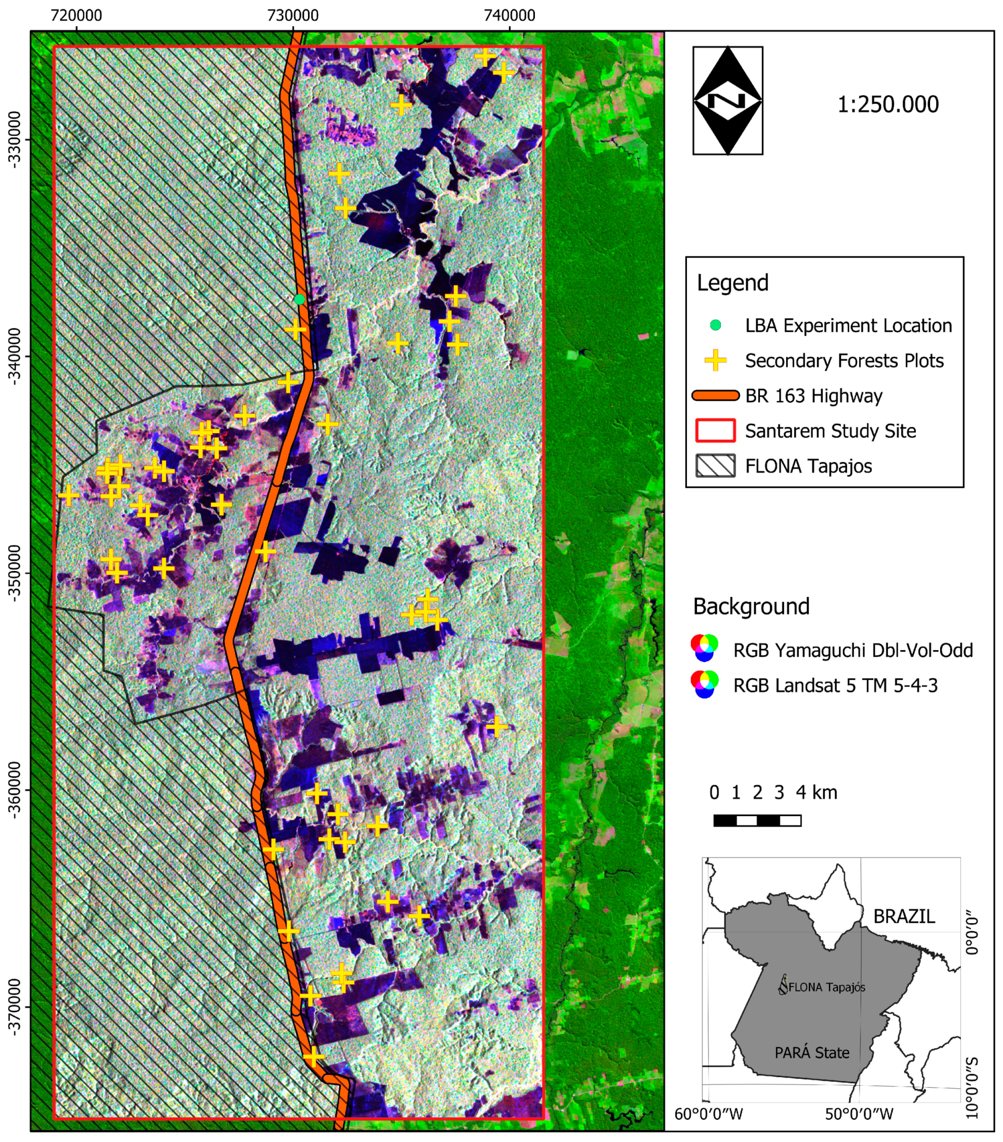
2.2. Site Description

The climate is classified as Am by Köppen climatic definition, with mean annual temperature between 25.5 and 26.7 °C [51,52]. According to Chave et al. [53], Santarém site is considered moist forest located in areas with annual rainfall between 1500 and 2500 mm and dry season length <5 months. The dry season, considering average monthly rainfall lower than 100 mm, occur from July to November. The soils are predominantly Oxisols (red-yellow Latosols), with low cation exchange capacity, high saturation by exchangeable aluminum Al+++, low pH, and are mainly found in non-flooded upland Terra-firme areas [54]. In a lesser proportion than Oxisols, Ultisols (Argisols) occurs in lowland and floodplain areas, which are also nutrient poor and often sandier [55,56,57]. The terrain is flat to undulate and the altitude is 100 m above sea level [58].

The vegetation prior to deforestation is classified as dense ombrophilous forest of Terra-firme and open rain forest composed of palm trees in the sandy soils as Attalea speciosa Mart. (Babaçu) and A. maripa (Aubl.) Mart. (Inajá) ([21,59], author’s observations). Dense ombrophilous forest of Terra-firme presents a bi-modal distribution of tree-canopy height, one stratum formed by emergent trees as Manilkara huberi (Ducke) Chev. (Maçaranduba) and Hymanaea courbaril L. (Jatobá) with an average height of 35–40 m and a lower stratum made of sub-dominant trees (average height = 15–30 m) [60,61,62]. The SFs, however, show a unimodal distribution of tree-height with mean 14.3 m where emergent trees are rare and represented by small individuals [63]. The species density ranged between 133 and 186 sp ha⁻¹, and the tree density is 441 ± 43 ind ha⁻¹ with the most prominent families being Lechytidaceae and Fabaceae [51,60,61].

2.3. Field and Satellite Imagery Data

The processing steps of field inventory and ALOS-2 PALSAR-2 data are shown in Figure 2 and are described in the following sections.

Field plot data were composed by two databases: 16 plots measured in this study and 26 plots measured by Silva [64] (

Table 1. Field plot information by age, diameter at breast height (DBH at 1.3 m height), inventory date, succession class, area, and plot size.

N	Plot Size (m)	DBH min (cm)	Age (Years)	Inventory Date (Year)	Succession	Area (ha)	Reference
16	10 × 100	5	16–28	2015	Advanced (Adv)	1.60	Our study
16	20 × 100	10	16–28	2015	Advanced (Adv)	3.20	Our study
16	60 × 100	20	16–28	2015	Advanced (Adv)	9.60	Our study
14	20 × 50	5	1–7	2012/13	Initial (ISS)	1.75	Silva et al. [64]
9	20 × 50	5	7–16	2012/13	Intermediate (IntSS)	2.40	Silva et al. [64]
3	25 × 100	10	>16	2012/13	Advanced (Adv)	1.35	Silva et al. [64]

). The sample plots were placed close to the FLONA of Tapajós on either side of the BR-163 highway, 100 km to the south of the city of Santarém (Figure 1).

In this study, we measured 16 nested plots of 60 × 100 m in advanced SFs (>16 years) during September 2015. In the nested plots, all trees with a diameter at the breast height (DBH at 1.3 m height) greater than or equal to 5 cm were measured within a 10 m × 100 m plot size. Trees with a DBH ≥ 10 cm were measured in a 20 m × 100 m plot size, and trees with a DBH ≥ 20 cm were measured in a 60 m × 100 m plot size.

Silva [64] carried out a field campaign between 2012 and 2013 at the same site (Table 1). The method consisted of the collection of 23 plots (20 m × 50 m) for the SF with initial secondary succession (ISS) and intermediate secondary succession (IntSS), and three plots for the advanced SF (25 m × 100 m). In both databases, all individuals were identified at the species level.

2.4. Aboveground Biomass (AGB) Allometric Equations

The total AGB is composed by the sum of three components of the forest plots: the living tree AGB, the palm AGB, and the standing dead tree AGB. Each of these components was addressed separately and has their own allometric equations for AGB estimation. The total AGB, hereafter named AGB, was then extrapolated to unit area (Mg ha⁻¹).

We evaluated 23 allometric equations to estimate AGB that are available from the literature for primary and secondary forests, and compared the equations’ estimates with those from 148 harvested trees [65,66]. All tested equations underestimated AGB, but the equation from Brown et al. [67] presented the lowest relative root mean square error (RMSE = 14%, obtained by the ratio between the RMSE and the average observed AGB). The underestimation was due to the errors concerning individuals with DBH 30 cm whose values were superior to 400 kg and to the high number of PFs species in the harvested trees. Hence, living AGB was estimated with the equation developed by Brown et al. [67] (1)

$${\mathrm{AGB}}_{\mathrm{live}}=\exp \left(-2.41+0.9522\ln \left({\mathrm{DBH}}^2 \mathrm{h} \mathsf{\rho }\right)\right)$$

(1)

where AGB is the live aboveground biomass in kg, DBH in cm, h is the total height estimated by hypsometric equations adjusted by ecological species groups by Cassol et al. [63], and ρ (rho) is the wood density collected from the literature and from the Global Wood Density Database [63,68]. Palm AGB was measured with distinct equations according to Table S1, Supplementary Materials.

The AGB of standing dead trees was estimated with Equation (1) using a rotten wood density ρ = 0.342 g cm⁻³ and with the equations in the Table S1, Supplementary Materials for dead palms using ρ = 0.327 g cm⁻³ [69].

The SF plots provided by Silva et al. 2016 had their AGB estimated by Uhl equation [18] (2)

$${\mathrm{AGB}}_{\mathrm{live}}=\exp \left(-2.17+1.02\ln \left({\mathrm{DBH}}^2\right)+0.39\ln \left(\mathrm{h}\right)\right)$$

(2)

2.5. Growth Models for Biophysical Variables

The SF growth was modeled to project the estimates of the biophysical variables to the SAR acquisition year in order to avoid temporal mismatch between both datasets, and also to provide the accumulation rates of these variables by age. Otherwise, the data from SAR could not be representative of the structural biophysical variables at the exact acquisition time, due to fast forest growth on these areas. The biophysical variables modeled were: the mean diameter (DBH), the mean total height (Ht), the basal area (G), the tree density (N), the species richness (S) and the aboveground biomass (AGB). The selected growth yield model was Chapman-Richards (8) as [70] (3)

$${\mathrm{Y}}_{\mathrm{t}}=\mathrm{A}{\left(1-{\mathrm{e}}^{-\mathrm{kt}}\right)}^{\mathrm{c}}+\mathsf{\epsilon }$$

(3)

where Yt represents the size of the variable at age t; A refers to the asymptote (maximum value of Y when the age tends to the infinite), the coefficient k is the growth rate of Y as a function of time t, c is the shape of the curve (inflection point), and ε is the experimental error. The negative exponential was used to estimate N (4) as [25]

$$\mathrm{N}={\mathrm{N}}_{\mathrm{a}}+\left({\mathrm{N}}_0-{\mathrm{N}}_{\mathrm{a}}\right){\mathrm{e}}^{-\mathrm{kt}}+\mathsf{\epsilon }$$

(4)

where ${\mathrm{N}}_0$ is the asymptote (tree density per hectare at t = 0), ${\mathrm{N}}_{\mathrm{a}}$ is the tree density per hectare at t = ∞, k is the decrease rate of N at time t. The parameters of the (3) and (4) were adjusted using the non-linear least squares method [71].

The input data for the growth models were obtained from SFs data located in Santarém region with ages varying from 1 to 30 years [72,73,74], along with the field plots measured in the present study. Plots obtained from these studies vary according to size, age, and methodology of measurement, but were carried out under similar environmental conditions (same geographic location)—first model assumption. However, the high variability of the dataset may result in the non-convergence of the growth model parameters; and a simple solution is to hold fixed each one of the model parameters, usually the asymptote [75]. Thus, we assumed that the asymptote (A, N, or ${\mathrm{N}}_0$) of each biophysical parameter of the SF resembles the values of adjacent PF—second model assumption [25]. These maximum values were obtained from the literature and correspond to the mean value observed in the PFs located nearby the study area (

Table 2. Asymptote of the biophysical variables in the primary forest used for modeling the secondary forest growth.

Biophysical Variables	Asymptote	Units	References
Mean diameter (DBH)	23.1	cm	[25,58,79,80,81,82,83,84]
Mean total tree height (Ht)	25.0	m	[25,79,82,85,86]
Basal area (G)	24.4	m2 ha−1	[25,79,82,85,87,88,89,90,91]
Species richness (S)	133.00	sp ha−1	[60]
Tree density (N)	433.00	individuals ha−1	[25,60,80,82,88,90,91]
Aboveground biomass (ABG)	314.00	Mg ha−1	[25,60,61,79,92]

). In this scope, were considered as PFs the forests that have never been clear cut in the Landsat time-series, according to the references of the Table 2. The goodness-of-fit of the Chapman-Richards models was evaluated according to the significance and the confidence interval of their parameters. Moreover, a visual analysis of their residuals was performed [76,77].

From the adjusted models, the accumulation rates of the biophysical variables were obtained through the partial derivatives of the growth curves. The mean annual increment (MAI) was obtained by the derivative of the second order, or simply by dividing the estimated value by the corresponding age [78]. The age at which SF growth rate is maximum (maximum MAI) was then estimated according to the MAI curves.

2.6. Landsat Time-Series Classification

Landsat data acquired over this site between 1984 and 2003 (

Table 3. Landsat 5 Thematic Mapper (TM) and Landsat 7 Enhanced TM plus (ETM+) data acquired over the Santarém site (Path 227, Row 62).

Date	Sensor	Date	Sensor	Date	Sensor
24 August 1984	TM	20 October 1993	TM	29 August 2003	TM
26 July 1985	TM	10 October 1995	TM	1 July 2005	TM
29 July 1986	TM	25 August 1996	TM	5 August 2006	TM
16 July 1987	TM	27 July 1997	TM	21 June 2007	TM
3 August 1988	TM	15 August 1998	TM	30 November 2008	TM
22 August 1989	TM	3 September 1999	TM	12 July 2009	TM
9 August 1990	TM	5 September 2000	TM	29 June 2010	TM
11 July 1991	TM	16 September 2001	ETM+

) were classified as PFs, non-forest and SFs using a fuzzy logic approach that was applied to the red (0.63–0.69 μm), near-infrared (0.76–0.90 μm), and shortwave infrared (1.55–1.77 μm) Landsat bands as well as derived fractional images from [93] (shade/moisture, vegetation, and soil) [21]. The time-series images were acquired by the USGS and were orthorectified and calibrated to units of spectral radiance (W m⁻² sr⁻¹ μm⁻¹); then they were calibrated to top of atmosphere (TOA) reflectance using calibration factors and equations provided by Chander et al. [94].

This time-series of land cover maps was extended to the period 2005–2010 and image classification of Landsat imagery was done with a machine learning algorithm (random forests) by Carreiras et al. [28]. The time-series were updated by visual interpretation only in the place where the sample plots were allocated.

Landsat time-series were used to extract the land-use history in SFs, such as the age, the period of active land-use (PALU), and the frequency of cuts (FC), according to methodology described in Carreiras et al. [28]. The SF age was defined by age since the last deforestation event, PALU is the period of active land use for agriculture or livestock practices, in years, and FC is the number of deforestation events (clear cut events).

2.7. ALOS-2 PALSAR-2 Data Processing

Two quad-pol scenes covering the study site were acquired in CEOS SAR format Single Look Complex (SLC) at processing level 1.1 in slant range and HBQ mode of acquisition (high sensitivity). SAR images were acquired at descending orbit in a right-looking off nadir angle (θ) of 28–31°. The SLC nominal resolution is 2.86 m and 3.13 m in range and azimuth respectively. Both scenes were acquired at the end of rainy season (6 February 2015) (Table S2, Supplementary Materials).

The cumulative rainfall on the date of acquisition and the day before was 10 mm [95]. The low accumulated precipitation at the previous date, however, should not cause major problems related to the increase in dielectric constant given the high evaporation in this season (about 3.5 mm day⁻¹), which partially cancels the cumulative rainfall.

In orbital low-frequency SAR systems, the path of the microwave pulse traverses twice the ionosphere, a region of free electrons pervaded by the magnetosphere resulting in the rotation of the plane of the polarization wave, known as Faraday rotation (FR) [96]. The magnitude of the FR depends on a number of factors, including RADAR wavelength, degree of ionization, solar activity, geographic position, and total electron content (TEC) at the acquisition date. The TEC is defined as the amount of free electrons in the ionosphere magnetic field and causes an increase in the FR angle (Ω). Due to intense solar activity, the TEC observed at the acquisition date was high, circa 70 × 10¹⁶ electrons m⁻², which resulted in a FR angle of approximately 15° in the plane of transmitted wave polarization and around 30° considering the transmitted and received wave [96,97,98].

According to Wright et al. [98], angles of rotation greater than 8.3° may reduce the accuracy of biophysical variables estimation. FR was previously corrected in one of the scenes, but preliminary analysis of the corrected data showed no significant changes in the polarimetric responses of the main forest targets. Therefore, we did not perform the FR correction in order to avoid unnecessary transformation of the coherence matrix, although we believe this correction is necessary when SAR data from different orbits and dates will be used for classification purposes.

Image processing consisted of the following procedures: multilooking, polarimetric filtering, extraction of attributes derived from covariance and coherency matrices, polarimetric decompositions, calibration, and finally geocoding (Figure 2).

The azimuth and range resampling factor (multilooking) was set at 2:1, resulting in a ground spatial resolution of approximately 6.25 m. Although multilooking is a process of de-speckling, we also performed a polarimetric filtering to further reduce speckle noise.

Since the size of the forest plots are several orders of magnitude greater than the SAR spatial resolution (10–15 times), we have tested different filter sizes with the objective of finding the most suitable window size for de-speckling. So, we used a Refined Lee polarimetric filter, tested 10 different filter sizes from 3 × 3 to 21 × 21 pixels, and compared the resulting of the mean intensity backscattering in all polarizations with the observed AGB (Supplementary Materials, Figure S1).

The optimal window size was set up to 11 × 11 pixels, selected by looking at the mean relative growth of R² between filters of different sizes and the AGB at plot level (Figure S1). This optimal window size was a trade-off between the gain obtained by the de-speckling caused by indiscriminate increase of the filter size and the loss of relevant radiometric information caused by spatial smoothing [65].

Several attributes from the coherency and covariance matrices and polarimetric decompositions were obtained using PolSARpro 5 (https://earth.esa.int/web/polsarpro/home) for characterizing SF and modeling forest AGB, generating 125 polarimetric attributes (

Table 4. Polarimetric attributes description.

Input Matrix	N°Attr.	Polarimetric Attributes	Reference
C3	9	I_C11, I_C12imag, I_C12real, I_C13imag, I_C13real, I_C22, I_C23imag, I_C23real, I_C33	[104]
C3	3	Freeman_Dbl, Freeman_Odd, Freeman_Vol	[105]
C3	2	ρhh-vv, |ρhh-vv|	[104]
C3	3	Neumann_mDelta, Neumann_phDelta, Neumann_tau	[106]
C3	3	VanZyl_Dbl, VanZyl_Odd, VanZyl_Vol	[107]
C3	4	Yamaguchi_Dbl, Yamaguchi_Hlx, Yamaguchi_Odd, Yamaguchi_Vol	[108]
C3	4	Bhattacharya_Dbl, Bhattacharya_Hlx, Bhattacharya_Odd, Bhattacharya_Vol	[109]
C3	5	MCSM_Dbl, MCSM_DblHlx, MCSM_Odd, MCSM_Vol, MCSM_Wire	[110]
C3	4	Singh_Dbl, Singh_Hlx, Singh_Odd, Singh_Vol	[111]
S, T3	16	TSVM_alpha_s, TSVM_alpha_s1, TSVM_alpha_s2, TSVM_alpha_s3, TSVM_phi_s, TSVM_phi_s1, TSVM_phi_s2, TSVM_phi_s3, TSVM_psi_s, TSVM_psi_s1, TSVM_psi_s2, TSVM_psi_s3, TSVM_tau_s, TSVM_tau_s1, TSVM_tau_s2, TSVM_tau_s3	[112]
T3	9	T11, T12imag, T12real, T13imag, T13real, T22, T23imag, T23real, T33	[104]
T3	15	A, H, α, β, λ, γ, δ, p1, p2, p3, HA, H_A, λ1, λ2, λ3	[113]
T3	9	T11_H, T12imag_H, T12real_H, T13imag_H, T13real_H, T22_H, T23imag_H, T23real_H, T33_H	[114]
T3	9	T11_C, T12imag_C, T12real_C, T13imag_C, T13real_C, T22_C, T23imag_C, T23real_C, T33_C	[115]
T3	9	T11_B, T12imag_B, T12real_B, T13imag_B, T13real_B, T22_B, T23imag_B, T23real_B, T33_B	[116]
T3	6	SE, SE_norm, SE_I, SE_I_norm, SE_P, SE_P_norm	[117]
T3	4	SERD, SERD_norm, DERD, DERD_norm	[118]
T3	1	PH—pedestal height	[119]
T3	1	PF—polarization fraction	[120]
T3	1	RVI—radar vegetation index	[107]
C3	3	VSI—vegetation scattering index, BMI—biomass index, CSI—canopy structure index	[121]
C3	1	RFDI—radar forest degradation index	[122]
C3	1	Span (Total Power)	[104]
C3	2	Rpp—parallel polarization ratio, Rcp—cross-polarization ratio	[123]
C3	1	Forest	[124]

Note: C3—covariance 3 × 3 matrix, T3—coherency 3 × 3 matrix, S—Sinclair 2 × 2 matrix. The complete nomenclature of the variables is in Appendix A Table A1.

).

Calibration consists of converting digital numbers to backscatter coefficient σ° (sigma-naught, in dB) in the four polarizations, and was calculated by (5) [101 < 99]

σ° = 10 log10 (I² + Q²) + CF

(5)

where I and Q are the phase image and complex image phase quadrature (SLC), respectively. CF is the calibration coefficient factor CF = −83 dB ± 0.406 dB [99].

After calibration and extraction of the polarimetric attributes, data was geocoded using the Range-Doppler rigorous method. This process performs the geocoding of the SAR data with the precise transformation of slant-range to ground-range using a digital elevation model (DEM) [100,101]. In this rigorous model, the backscattering from a point target is shifted in frequency by the proportion of the relative velocity between the satellite and target as a Doppler effect (6)

$${\mathrm{f}}_{\mathrm{DC}}=\frac{2}{\mathsf{\lambda }\mathrm{R}}\left(\overrightarrow{{\mathrm{V}}_{\mathrm{s}}}-\overrightarrow{{\mathrm{V}}_{\mathrm{t}}}\right).\left(\overrightarrow{{\mathrm{R}}_{\mathrm{s}}}-\overrightarrow{{\mathrm{R}}_{\mathrm{t}}}\right)$$

(6)

where ${\mathrm{f}}_{\mathrm{DC}}$ is the Doppler frequency of the returned echo, λ is the SAR wavelength, R is the sensor to target slant range, $\overrightarrow{{\mathrm{V}}_{\mathrm{s}}}$ and $\overrightarrow{{\mathrm{R}}_{\mathrm{s}}}$ are the vector velocity and position of the spacecraft, and $\overrightarrow{{\mathrm{V}}_{\mathrm{t}}}$ and $\overrightarrow{{\mathrm{R}}_{\mathrm{t}}}$ are the vector velocity and position of the target, respectively [100].

The unknown parameters are $\overrightarrow{{\mathrm{V}}_{\mathrm{t}}}$ and $\overrightarrow{{\mathrm{R}}_{\mathrm{t}}}$ which both can be obtained from a precise DEM that relates a pixel $\overrightarrow{\mathrm{P}}\left({\mathrm{P}}_{\mathrm{x}},{\mathrm{P}}_{\mathrm{y}}\right)$ on the SAR image with a correspondent pixel on the Earth surface by a revolution ellipsoid function model $\mathrm{f}\left(\mathsf{\lambda },\mathsf{\Phi },\mathrm{H}\right)$ as (7)

$$\overrightarrow{\mathrm{P}}\left({\mathrm{P}}_{\mathrm{x}},{\mathrm{P}}_{\mathrm{y}}\right)=\mathrm{f}\left(\mathsf{\lambda },\mathsf{\Phi },\mathrm{H}\right)= \frac{{\mathrm{p}}_{\mathrm{x}}^2+{\mathrm{p}}_{\mathrm{y}}^2}{\left(\mathrm{a}+\mathrm{h}\right)²}+\frac{{\mathrm{p}}_{\mathrm{z}}^2}{\left(\mathrm{b}\right)²}$$

(7)

where a and b are the major and minor axes of the revolution ellipsoid respectively, and h is the height of the pixel with respect to the ellipsoid. Finally, the backscatter in slant-range β is transformed into ground-range of the standard plot for a given local incident angle ${\mathsf{\theta }}_{\mathrm{i}}$ obtained from the DEM by (8) [102]

$$\mathsf{\sigma }°=\frac{\mathsf{\beta }°}{\mathrm{sen}\mathsf{\theta }}.\left({\mathrm{sen}\mathsf{\theta }}_{\mathrm{i}}/\mathrm{sen}\mathsf{\theta }\right)$$

(8)

In addition, the topographic effects are reduced by precise geocoding (Equations (6)–(8)), which are considered a source of associated uncertainty of the AGB estimation [37,103].

2.8. Correlation Analysis

Pearson’s correlation coefficient analysis was performed twice, namely: (1) to understand how the polarimetric attributes (SAR decompositions) are related to the biophysical variables (structure of the SFs) and also with the land-use history, and (2) to find the best subset of polarimetric attributes for retrieving AGB. In the first analysis (1), the adjusted biophysical, PALU, FC, and all polarimetric attributes were evaluated by the correlation matrix pairwise. Only the highest Pearson correlation coefficients are showed and the p-value is provided.

For the second analysis (2), a correlation-based feature selection (CFS) filter algorithm [125] was applied in order to reduce the dimensionality of the data in the FSelector package from R [126]. In the CFS approach, an algorithm selects a subset of attributes based on the correlation coefficients and the concept of information entropy theory. The metrics of Yang and Pedersen [127], such as information gain and chi-square test (χ²), were used to measure the degree of association between the class of intensity used and the attributes, as well as the interrelationship among attributes. The best subset of data is formed by the attributes having higher correlation and greater gain of information with the class and having also lower correlation amongst them [125,128].

2.9. Models to Retrieve Aboveground Biomass

We evaluated the performance of two different types of regression models for AGB estimation: (i) non-linear and (ii) multiple linear. Goodness-of-fit was calculated using (i) the significance and confidence interval of the regression parameters, (ii) the distribution of the standardized residuals from the regression to verify the presence of possible outliers, (iii) the Akaike information criterion (AIC), and (iv) the Breusch–Pagan test to evaluate the homoscedasticity of the residuals [76].

2.9.1. Non-Linear Regression Model

The non-linear regression model involves the logarithmic relationship between AGB (Yi) and a single independent variable (X), usually the backscatter coefficient, given by (9) [77]

$${\mathrm{Y}}_{\mathrm{i}}=\mathrm{E}\left({\mathrm{Y}}_{\mathrm{i}}{|\mathrm{X}}_{\mathrm{i}}\right)+{\mathsf{\epsilon }}_{\mathrm{i}}=\mathrm{f}\left({\mathrm{X}}_{\mathrm{i}},{\mathsf{\theta }}_{\mathrm{i}}\right)+{\mathsf{\epsilon }}_{\mathrm{i}}$$

(9)

whereby ${\mathrm{Y}}_{\mathrm{i}}$ is the average of the i-th AGB observations $\mathrm{E}\left({\mathrm{Y}}_{\mathrm{i}}{|\mathrm{X}}_{\mathrm{i}}\right)$ depend on ${\mathrm{X}}_{\mathrm{i}}$ in Mg ha⁻¹, by means of a mean kernel function of $\mathrm{f}\left({\mathrm{X}}_{\mathrm{i}},{\mathsf{\theta }}_{\mathrm{i}}\right)$; ${\mathrm{X}}_{\mathrm{i}}$ is the explanatory variable that can have one or more components and ${\mathsf{\theta }}_{\mathrm{i}}$ is the parameter vector. ${\mathsf{\epsilon }}_{\mathrm{i}}$ is the random error with mean $\mathrm{E}\left\{{\mathsf{\epsilon }}_{\mathrm{i}}\right\}=0$ and variance ${\mathsf{\sigma }}^2\left\{{\mathsf{\epsilon }}_{\mathrm{i}}\right\}={\mathsf{\sigma }}^2/\mathrm{w}$ by the non-linear least squares method. For many practical applications, w, which is the weight given to the variance, is equal to one. Non-linear models were fit with the “nls” package in R.

2.9.2. Multiple Linear Regression Model

In a multiple linear regression model, the dependent variable AGB (Yi) is estimated by multiple independent variables (Xi) from the SAR data by a linear (in the parameters) relationship with these variables (10)

$${\mathrm{Y}}_{\mathrm{i}}={\mathsf{\beta }}_0+{\mathsf{\beta }}_1{\mathrm{X}}_{\mathrm{i}1}+{\mathsf{\beta }}_2{\mathrm{X}}_{\mathrm{i}2}+\dots +{\mathsf{\beta }}_{\mathrm{p}-1}{\mathrm{X}}_{\mathrm{i},\mathrm{p}-1}+{\mathsf{\epsilon }}_{\mathrm{i}}$$

(10)

where ${\mathrm{Y}}_{\mathrm{i}}$ is AGB at the i-th observation in Mg ha⁻¹, ${\mathsf{\beta }}_0$, ${\mathsf{\beta }}_1$,…, ${\mathsf{\beta }}_{\left(\mathrm{p}-1\right)}$ are the model parameters and ${\mathrm{X}}_{\mathrm{i},\mathrm{p}-1}$ are the p − 1 explanatory variables (polarimetric attributes, Table 4) at the i-th observation, and ${\mathsf{\epsilon }}_{\mathrm{i}}$ is the random error with mean $\mathrm{E}\left\{{\mathsf{\epsilon }}_{\mathrm{i}}\right\}=0$ and variance ${\mathsf{\sigma }}^2\left\{{\mathsf{\epsilon }}_{\mathrm{i}}\right\}={\mathsf{\sigma }}^2$.

Multiple linear models were fit with the ordinary least squares (OLS) method. The analysis was performed using the exhaustive selection package “Glmulti” implemented in R [129]. The selection of the model was performed by the AIC criterion, whose models with ∆AIC < 2 were chosen; and the best model was determined by the weights given to the set of explanatory variables in the model. The greater the weight, the greater the contribution of each variable to the model. The selection of optimal subset was performed by CFS selector in order to reduce the input polarimetric attributes and to avoid overfitting of the MLR [76].

2.10. Evaluation of Model’s Performance

Validation of the regression models was carried out by assessing the distribution and coefficient of determination (R²) between predicted and reference values (from the validation sample). The root mean square error of bias and variance terms following reference [130] (11)

$$\mathrm{RMSE}=\sqrt{{\mathrm{bias}}^2+\mathrm{variance}}$$

(11)

In addition, the error distribution was presented for each model and the null hypothesis of the deviation (bias), which states that the estimate is equal to zero (without trend), was analyzed by the one-sample t-test. The number of plots was small (n = 42), thus limiting the separation in training and validation subsets. Therefore, a bootstrapping randomization process with 100 repetitions was carried out, maintaining the separation of 80% for training and 20% for validation.

3. Results

3.1. Structural Parameters of the Secondary Forests

The values of structural parameters, such as the mean diameter, tree height, basal area, and biomass increased with forest age and secondary succession stages (

Table 5. Mean and standard deviation (in brackets) of structural parameters in secondary forest plots by succession class: ISS—initial secondary succession, IntSS—intermediate secondary succession, and AdvSS—advanced secondary succession. The abbreviations are: FC—frequency of cuts, PALU—period of active land-use, DBH—diameter at the breast height, Ht—total height, G—basal area, S—species density, N—tree density, AGB—aboveground biomass.

Plot	n	Age *	FC	PALU	DBH	Ht	G	S	N	AGB
	(Plots)	(Years)	(x)	(Years)	(cm)	(m)	(m2 ha−1)	(sp ha−1)	(ind ha−1)	(Mg ha−1)
ISS	14	3.3(1.1)	2.8(0.5)	3.1(1.7)	11.9(2.8)	13.0(1.4)	14.0(5.6)	29(9)	841(145)	83.2(42.2)
IntSS	9	9.2(2.3)	2.2(1.1)	2.8(1.9)	12.9(1.1)	13.5(0.5)	16.7(2.3)	31(4)	785(57)	99.3(17.8)
Adv	19	20.2(2.6)	1.9(0.9)	1.4(0.5)	17.0(2.3)	15.0(1.1)	24.9(3.8)	49(7)	1274(424)	151.5(30.4)
Mean	42 †	12.2(7.9)	2.3(1.1)	2.3(1.5)	14.4(3.3)	14(1.5)	19.5(6.5)	39(12)	1025(373)	117.2(45.2)

Note: * Age at the field survey. ^† total.

). The exception was the tree density, which showed the lowest value in the intermediate secondary succession 785 ± 57 individuals (ind) ha⁻¹ (Table 5). For instance, the initial secondary succession (ISS) had, on average, 83 Mg ha⁻¹ of AGB and 3.3 ± 1.1 years, the intermediate secondary succession (IntSS) had 99 ± 18 Mg ha⁻¹ and 9.2 ± 2.3 years, and the maximum AGB was observed at a 28 years old secondary forest plot (AGB = 200.0 Mg ha⁻¹). The average AGB in the ISS was 55% lower than in the Adv. succession, and 20% lower than in the IntSS (Table 5). Due to the short time interval of land-use history, the PALU and FC were higher in the ISS and IntSS classes.

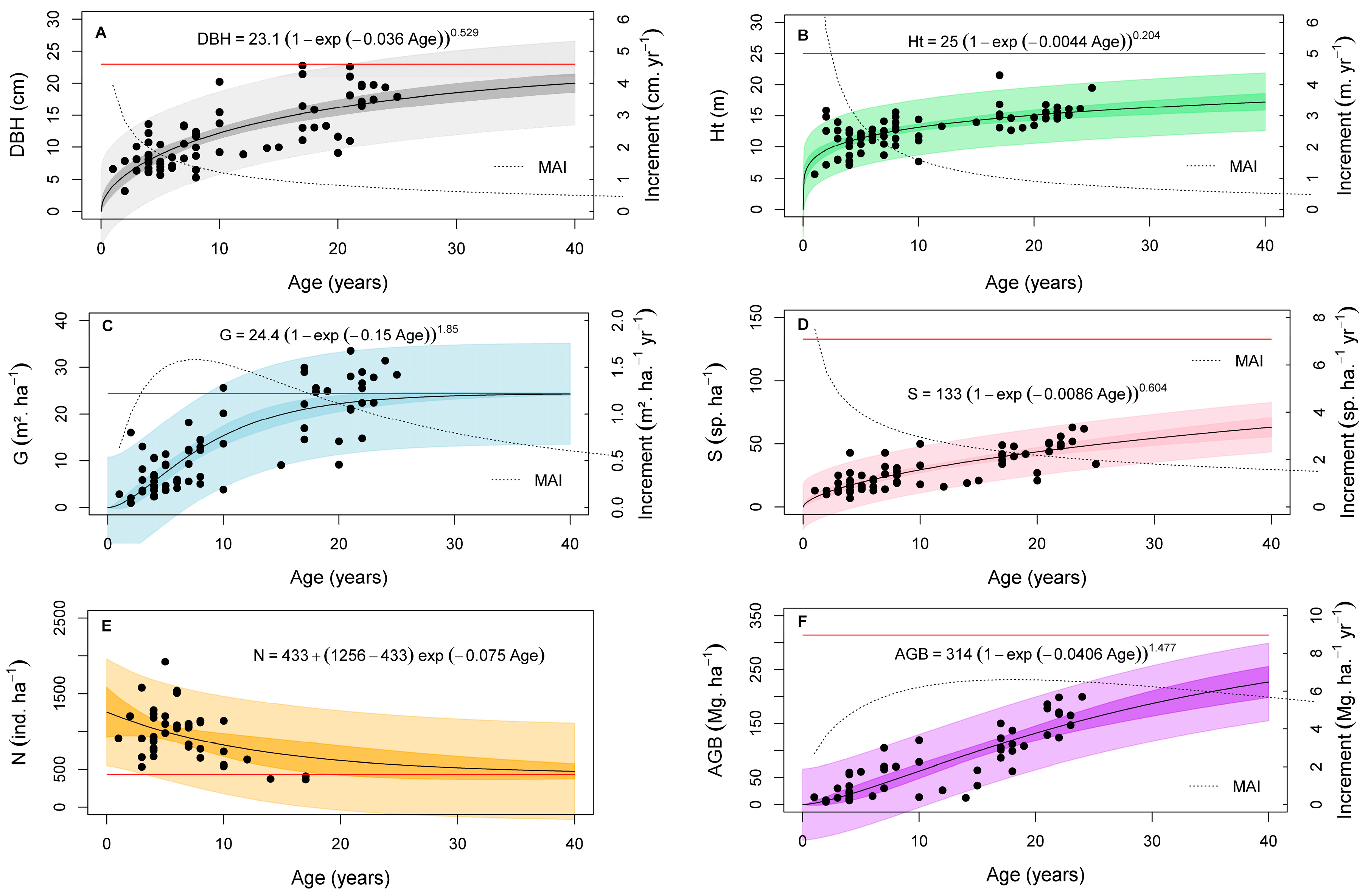
3.2. Growth Models and Accumulation Rates of the Secondary Forests Biophysical Variables

The curves of biophysical variables showed different behavior, indicating distinct accumulation rates. The fitted growth models for mean diameter (DBH), mean forest tree-height (Ht), and species richness (S) did not show a typical sigmoidal shape, but resembled a logarithmic model—inflection point c < 1 (Figure 3). As a consequence, the corresponding maximum MAI of these biophysical variables occurs in the first years of the forest life. All model parameters (A, k, and C) were significant for α = 0.05. For instance, mean DBH and mean Ht showed a rapid growth in the SFs of Santarém, reaching half of the PF value in approximately nine and eight years, respectively (Figure 3A,B). The MAI of mean DBH was higher than 2 cm year⁻¹ in the first five years (Figure 3A). The MAI of mean Ht was greater than 1 m year⁻¹ during the first 13–14 years (Figure 3B), with similar results reported by Neeff and Santos [25].

The basal area (G) was the biophysical parameter that reached the asymptote faster in the SFs, as reported by other authors [12,131]. For instance, SFs recover 90% of G observed in adjacent PF at 19 years age (Figure 3C). The maximum MAI of G was estimated at 1.6 m² ha⁻¹ year⁻¹ and occurred in the fourth year, while [25] observed maximum MAI in the sixth year. Along with the Ht and G, the tree density (N) quickly reached values close to the PFs [25,131]. At the age of 20, SFs have 70% N of the PF (Figure 3E). Due to different measurements methodologies regarding minimum DBH measured, we excluded some advanced SF aging plots >20 years from the analysis of tree density.

The S, on the other hand, showed the slowest accumulation rate in the SFs amongst the biophysical variables; the MAI of S was below to 4 sp ha⁻¹ year⁻¹ in the first 10 years and inferior to 2 sp ha⁻¹ year⁻¹ from the age of 25 years (Figure 3D). In this S recovery rate, the SFs of the Santarém site would present 72% of the S per hectare observed in the PF at approximately 100 years.

The mean AGB showed intermediate recovering rate. The MAI of AGB occurs at 18th year MAI = 6.6 Mg ha⁻¹ year⁻¹ (Figure 3F). At this growth rate, 50% of the asymptote can be reached at age 25; and 75% at age 44. Considering that approximately 50% of the AGB is organic carbon (C), the potential assimilation of C is greater than 3.7 Mg C ha⁻¹ year⁻¹ in the Santarém SF up to 10 years-old.

3.3. Characterization of Secondary Forest with Polarimetric Data

The polarimetric attributes have showed different responses or sensitivity for each biophysical variable, given by the Pearson’s correlation coefficient (Figure 4). For instance, the third eigenvalue, associated to the respective eigenvector of the Cloude decomposition (λ3), is related to the magnitude of the cross-polarization signal (HV) and showed the highest correlation ρ ≈ 0.6 with DBH, Ht, G, S, and AGB. With the exception of N, these biophysical variables obtained high ρ with the polarimetric attributes related to volumetric scattering, such as λ3, I_C22, the Forest index, and the volumetric scattering mechanisms of Singh, Freeman–Durden, and Yamaguchi decompositions (Figure 4). The term I_C22 refers to second element of the diagonal of the covariance matrix [C]₃ ${\mathrm{C}}_{22}=2⟨{\left|{\mathrm{S}}_{\mathrm{HV}}\right|}^2⟩$ and the Forest index refers to the contribution of volumetric and surface backscattering from forest canopies [124] by (12)

$${\mathsf{\sigma }}_{\mathrm{forest}}^0={\mathsf{\sigma }}_{\mathrm{hv}}^0+{\mathsf{\sigma }}_{\mathrm{hh}}^0.\frac{{\mathsf{\sigma }}_{\mathrm{hh}}^0}{{\mathsf{\sigma }}_{\mathrm{hv}}^0}$$

(12)

where ${\mathsf{\sigma }}_{\mathrm{forest}}^0$ is the backscattering from forest canopy, ${\mathsf{\sigma }}_{\mathrm{hv}}^0$ is the volumetric backscattering and ${\mathsf{\sigma }}_{\mathrm{hh}}^0$ is the surface backscattering.

As expected, the AGB, DBH, Ht, G, and S were positively correlated with the volumetric scattering, meaning that SFs areas presented greater volumetric scattering contribution with increasing forest age. However, the N showed no significant correlation with AGB, DBH, and Ht (p-value = 0.19, 0.28, and 0.76, respectively), and were weakly correlated with the SAR attributes. The highest correlation value with N (ρ = 0.30) was the real term off-diagonal of the covariance matrix ${\mathrm{C}}_{23}=\sqrt{2}⟨{\mathrm{S}}_{\mathrm{HV}}{\mathrm{S}}_{\mathrm{VV}}^{\ast }⟩$, although it was not significant at the α = 0.05 (Figure 4).

The land-use history of PALU and FC showed negative correlation with biophysical variables (Figure 4), which means that the longer is the PALU and higher is the FC the lower is the biophysical variables values in the SFs. The polarimetric attribute with the highest Pearson coefficient of PALU and FC was the Touzi target phase angle TVSM_phi_s (ρ = 0.37, p-value = 0.0.175 and ρ = 0.38, p-value = 0.014, respectively). Interestingly, the polarimetric attributes that were sensitive to the FC were angular decompositions as Touzi target phase angle (Φ_s), Touzi target ellipticity angle (τ_s), and Touzi target orientation angle (ψ_s).

The Touzi target phase angle showed a negative and significant correlation with PALU and FC, and also a positive and significant correlation with biophysical variables, being close to zero in high AGB. Touzi [112] described ${\mathsf{\varphi }}_{\mathrm{s}}=0$ as areas with ambiguity between dihedral-trihedral scattering types. SF areas subjected to a longer PALU and higher FC have greater contribution of trihedral scattering type, as shown by the distribution of Touzi target phase angle (${\mathsf{\varphi }}_{\mathrm{s}}$) (Figure 5).

3.4. Modeling AGB

The nonlinear (NL) model showed signal saturation for AGB values close to 150 Mg ha⁻¹ using the backscattering coefficient of the cross-polarized channel (σ⁰ HV), as has often been reported in the literature (Figure 6A). The fitted NL model has an AIC of 417.1 and low R² = 0.28 (

Table 6. Model’s performance evaluation. NL—nonlinear, MLR—multiple linear regression, RMSE—Root mean square error, ISS—initial secondary succession, IntSS—intermediate secondary succession, AdvSS—advanced secondary succession, PALU—period of active land-use.

	AIC	R2 Validation	RMSE (Mg ha−1)	RMSE ISS	RMSE IntSS	RMSE Adv	RMSE PALU 1–2 years	RMSE PALU 3–4 years	RMSE PALU >4 years	Bias (Mg ha−1)
NL	417.1	0.28	39.7	50.9	34.6	38.2	45.4	33.2	31.3	0.3
MLR	408.1	0.37	38.7	52.6	37.7	33.8	37.6	43.6	21.8	2.1

) when compared to other studies that used similar models R² = 0.44–0.86 [37,132,133]. We argue that this was due to the low amount of data available for the young SFs. In consequence, the mean error in the initial secondary succession (ISS) was higher than in the IntSS and advanced succession (Table 6). The RMSE from NL model represented about 12% of the mean value of the AGB (RMSE = 39.7 ± 6.8 Mg ha⁻¹, Table 6). The NL model had a bias of the estimate μ_bias = 0.26 ± 38.3 Mg ha⁻¹ and did not different from zero by the t-test (Figure 7I), besides of the tendency of overestimating the AGB > 150 Mg·ha⁻¹ (Figure 7A).

The young SFs have higher MAI of AGB and higher sensitivity to SAR microwave wavelength, which, in turn, has higher variability response of the radar signal than older SFs [25,39]. The standardized residues, otherwise, were heteroscedastic, rejecting the hypothesis of homoscedasticity of the residuals at the level α = 0.05 (BP: 4.8; p-value < 0.05, Figure 6B).

Due to the great number of polarimetric attributes tested (total of 125, Table 4 and Appendix A

Table A1. List of abbreviations, acronyms, and variables.

AdvSS	Advanced Secondary Succession
AIC	Akaike information criterion
ALOS-2	Advanced Land Observation Satellite-2
C, [C], [C]3	Covariance 3 × 3 matrix
CDB	Convention on Biological Diversity
CF	Calibration coefficient factor (dB)
CFS	Correlation-based feature selection
DEM	Digital elevation model
FC	Frequency of cuts (× times)
FLONA	National forest, in Portuguese
FR	Faraday rotation (Ω)
FRA	Forest resources assessment
I	Phase image
IntSS	Intermediate secondary succession
ISS	Initial secondary succession
LULUCF	Land use, land-use change, and forestry
MAI	Mean annual increment
MCSM	Multiple-component scattering model
MLR	Multiple linear regression
NL	Non-linear
OLS	Ordinary least squares
PALSAR-2	Phased Array L-band Synthetic Aperture Radar-2
PALU	Period of active land use (years)
PF	Primary forest
PRODES	Program for Monitoring Deforestation of the Amazon by Satellite
Q	Complex image phase quadrature
R	R Foundation for statistical computing
SAR	Synthetic aperture radar
SF	Secondary forest
SLC	Single look complex
T, [T], [T]3	Coherency 3 × 3 matrix
TanDEM	TerraSAR-X add-on for digital elevation measurement
TEC	Total electron content (electrons m−2)
TSVM	Target scattering vector model
VIF	Variance inflation factor
BP	Breusch–Pagan test
C	Organic carbon
CO2	Carbon dioxide
Mg	Mega grams (106 g)
Pg	Pentagrams (1015 g)
R2	Coefficient of determination
R2adj.	Coefficient of determination adjusted
RMSE	Root mean square error
|ρhh-vv|	Magnitude of complex coherency between linear polarizations (linear units) ([0, 1]; 0 = depolarized, 1 = completely polarized)
A	Asymptote
A	Anisotropy from Cloude & Pottier decomposition, related to the relative importance of secondary and tertiary scattering types A = (λ2 − λ3)/(λ2 + λ3)
AGB	Aboveground Biomass (kg or Mg ha−1)
alpha, α	Dominant scattering type angle in the trihedral-dihedral basis $\overline{\mathsf{\alpha }}={{\displaystyle \sum }}_{\mathrm{i}=1}^3{\mathrm{P}}_{\mathrm{i}}{\mathsf{\alpha }}_{\mathrm{i}}$ ([0, 90]; 0 = surface scattering, 45 = isotropic scattering (volumetric), 90 = double-bounce)
BMI	Biomass Index is an indicator of the relative amount of woody compared to leafy biomass $\mathrm{BMI}=\frac{{\sigma }_{\mathrm{hh}}^0+{\sigma }_{\mathrm{vv}}^0}{2}$
c	Shape of the curve (inflection point)
CSI	Canopy structure index is the relative importance of vertical versus horizontal structure in the vegetation $\mathrm{CSI}=\frac{{\sigma }_{\mathrm{vv}}^0}{{\sigma }_{\mathrm{vv}}^0+{\sigma }_{\mathrm{hh}}^0}$
DBH	Diameter at the breast height (cm)
DERD, DERD_norm	Double-bounce Eigenvalue relative difference, and normalized DERD ([0, 1]; 0 = 0 = multiple scattering mechanism, 1 = dominant double-bounce scattering)
Forest	Forest backscattering coefficient ${\sigma }_{\mathrm{forest}}^0={\sigma }_{\mathrm{hv}}^0+{\sigma }_{\mathrm{hh}}^0.\frac{{\sigma }_{\mathrm{hh}}^0}{{\sigma }_{\mathrm{hv}}^0}$
G	Basal area (m2 ha−1)
h	Tree height (m)
H	Entropy from Cloude & Pottier decomposition ([0, 1]; 0 = dominant scattering mechanism targets, 1 = random distributed targets) $\mathrm{H}=-{\displaystyle \sum }_{\mathrm{i}=1}^3{\mathrm{P}}_i\mathrm{lo}{\mathrm{g}}_3{\mathrm{P}}_i$
H_A	H(1–A) highlights a random scattering process (high H and low A, λ1, λ2, λ3
HA	H(A) highlights the presence of two scattering mechanisms with same pseudo-probabilities, high H and A, as forest targets ~λ3
Ht	Mean total tree height (m)
I_Cnm_imag, Cnm_imag	Imaginary term nm (row × column) of the covariance matrix (linear units)
I_Cnm_real, Cnm_imag	Real term nm (row × column) of the covariance matrix (linear units)
k	Growth rate
N	Tree density (ind ha−1)
N0	Tree density at t = 0
Na	Tree density at t = ∞
Neumann_mDelta	Scattering anisotropy magnitude from Neumann decomposition ([0, 2]; 0 = isotropic sphere, 1 = dipole) $\left|\delta \right|=\sqrt{\frac{⟨{\left|S_{\mathrm{hh}}-S_{\mathrm{vv}}\right|}^2⟩.⟨{\left|S_{\mathrm{hv}}\right|}^2⟩}{⟨{\left|S_{\mathrm{hh}}+S_{\mathrm{vv}}\right|}^2⟩}}$
Neumann_phDelta	$\mathrm{Phase} \mathrm{anisotropy} \arg (\mathsf{\delta }) \mathrm{from} \mathrm{Neumann} \mathrm{decomposition} ([-1, 1];-1=\mathrm{preferred} \mathrm{vertical} \mathrm{orientation}, 1=\mathrm{horizontal} \mathrm{orientation}) \arg \mathsf{\delta }=\arg \left\{⟨(S_{\mathrm{hh}}+S_{\mathrm{vv}}){(S_{\mathrm{hh}}-S_{\mathrm{vv}})}^{\ast }⟩\right\}$
Neumann_tau	$\mathrm{Normalized} \mathrm{degree} \mathrm{of} \mathrm{orientation} \mathrm{randomness} \mathrm{from} \mathrm{Neumann} \mathrm{decomposition} ([0, 1]; 0=\mathrm{preferred} \mathrm{orientation} \mathrm{direction}, 1 =\mathrm{completely} \mathrm{random} \mathrm{orientation}) \mathsf{\tau }=\frac{1}{\mathsf{\pi } p_{\mathsf{\psi }}(\overline{\mathsf{\psi }})}$
P	$\mathrm{Power} \mathrm{image} \mathrm{of} \mathrm{polarimetric} \mathrm{decomposition} P=P_s+P_d+P_v$
Ps	Proportion of odd-bounce or superficial scattering mechanism
Pd	Proportion of double-bounce scattering mechanism
Pv	Proportion of volumetric scattering mechanism
p1, p2, p3	Pseudo-probabilities of eigenvalues λi from Cloude & Pottier decomposition ([0, 1])
PF	Polarization fraction given by the difference between completely depolarized waves ([0, 1]; 0 = random distributed targets, 1 = dominant (pure) targets) $\mathrm{Fp}=1-(\frac{3{\mathsf{\lambda }}_3}{{\mathsf{\lambda }}_1+{\mathsf{\lambda }}_2+{\mathsf{\lambda }}_3})$
PH	$\mathrm{Pedestal} \mathrm{height} \mathrm{is} \mathrm{the} \mathrm{ratio} \mathrm{between} {\mathsf{\lambda }}_3 \mathrm{and} {\mathsf{\lambda }}_1 \mathrm{eigenvalues} \mathrm{from} \mathrm{Cloude} \& \mathrm{Pottier} \mathrm{decomposition}, \mathrm{or} \mathrm{contribution} \mathrm{of} \mathrm{depolarized} \mathrm{channel} \mathrm{PH}={\mathsf{\lambda }}_3/{\mathsf{\lambda }}_1$
phi, φ	Scattering type phase difference between trihedral-dihedral ([−90, 90]; 0 = phase ambiguity, −90° = trihedral, 90° dihedral)
psi, ψ	Target tilt angle related to orientation angle of SAR line-of-sight ([−45, 45]; ±45 = preferred orientation direction, 0 = completely random orientation)
Rcp	$\mathrm{Cross}-\mathrm{polarization} \mathrm{ratio} \mathrm{is} \mathrm{the} \mathrm{ratio} \mathrm{between} \mathrm{HV} \mathrm{and} \mathrm{HH} \mathrm{channel} (1 > \mathrm{higher} \mathrm{volumetric} \mathrm{contribution} \mathrm{in} \mathrm{relation} \mathrm{to} \mathrm{surface} \mathrm{scattering}) \mathrm{Rpc}=\frac{{\mathsf{\sigma }}_{\mathrm{hv}}^0}{{\mathsf{\sigma }}_{\mathrm{hh}}^0}$
RFDI	Radar Forest Degradation Index, is the normalized difference between σ0 hh and σ0 hv $([-1, 1]; 0>\mathrm{low} \mathrm{disturbed} \mathrm{forest}, <1 = \mathrm{high} \mathrm{disturbed} \mathrm{forest}) \mathrm{RFDI}=\frac{{\mathsf{\sigma }}_{\mathrm{hh}}^0-{\mathsf{\sigma }}_{\mathrm{hv}}^0}{{\mathsf{\sigma }}_{\mathrm{hh}}^0+{\mathsf{\sigma }}_{\mathrm{hv}}^0}$
Rpp	$\mathrm{Parallel} \mathrm{polarization} \mathrm{ratio} \mathrm{is} \mathrm{the} \mathrm{ratio} \mathrm{between} \mathrm{VV} \mathrm{and} \mathrm{HH} \mathrm{channel} (1 > \mathrm{dominant} \mathrm{double}-\mathrm{bounce} \mathrm{scattering}, <1 \mathrm{dominant} \mathrm{odd}-\mathrm{bounce} \mathrm{scattering}) \mathrm{Rpp}=\frac{{\mathsf{\sigma }}_{\mathrm{vv}}^0}{{\mathsf{\sigma }}_{\mathrm{hh}}^0}$
RVI	$\mathrm{Radar} \mathrm{vegetation} \mathrm{Index} \mathrm{given} \mathrm{by} \mathrm{the} \mathrm{backscattering} \mathrm{from} \mathrm{randomly} \mathrm{oriented} \mathrm{cylinders} ([0, 1.33]; 0 = \mathrm{thin} \mathrm{cylinders}, 1 = \mathrm{thick} \mathrm{cylinders}) \mathrm{RVI}= \frac{4{\mathsf{\lambda }}_3}{{\mathsf{\lambda }}_1+{\mathsf{\lambda }}_2+{\mathsf{\lambda }}_3}$
S	Species richness (sp ha−1)
SE	Shannon entropy, sum of the contribution of intensity (SE_I) and polarimetry (SE_P), in dB
SE_I, SE_I_norm	$\mathrm{Contribution} \mathrm{of} \mathrm{SE} \mathrm{intensity} \mathrm{normalized} ([0, 1]; 0 = \mathrm{low} \mathrm{coherent} \mathrm{entropy}, 1 = \mathrm{high} \mathrm{coherent} \mathrm{entropy}) S{E}_I=\log ({\mathsf{\pi }}^3{\mathrm{e}}^3{I}_T), \mathrm{IT}=\mathrm{Tr} [T]$
SE_P, SE_P_norm	Contribution of SE polarimetry normalized ([0, 1]; 0 = depolarized entropy, 1 = polarized entropy) $\mathrm{S}{\mathrm{E}}_{\mathrm{P}}=\log (1-{{\mathrm{p}}_{\mathrm{T}}}^2)$, ${\mathrm{p}}_{\mathrm{T}}=\sqrt{1-27\frac{\left|[\mathrm{T}]\right|}{\mathrm{Tr}{[\mathrm{T}]}^3}}$
SERD, SERD_norm	Single-bounce Eigenvalue relative difference, and normalized SERD ([0, 1]; 0 = multiple scattering mechanism, 1 = dominant single-bounce scattering)
Span	$\mathrm{Span} \mathrm{image} \mathrm{or} \mathrm{power} \mathrm{image} \mathrm{is} \mathrm{equal} \mathrm{to} \mathrm{the} \mathrm{sum} \mathrm{of} \mathrm{the} \mathrm{three} \mathrm{backscattering} \mathrm{coefficients} \mathrm{Span}={\left|{\mathsf{\sigma }}_{\mathrm{hh}}^0\right|}^2+2{\left|{\mathsf{\sigma }}_{\mathrm{hv}}^0\right|}^2+{\left|{\mathsf{\sigma }}_{\mathrm{vv}}^0\right|}^2$
t	Age
tau, τ	Helicity angle related to assess target symmetry ([−45, 45] 0 = symmetric target angle, ±45 = non-symmetric target angle)
Tnm_imag_Z	Imaginary term nm (row × column) of the coherency matrix from the Z decomposition, in linear units
Tnm_real_Z	Real term nm (row × column) of the coherency matrix from the Z decomposition, in linear units
VSI	Vegetation Scattering Index is an indicator of canopy thickness or density $\mathrm{VSI}=\frac{{\mathsf{\sigma }}_{\mathrm{hv}}^0}{{\mathsf{\sigma }}_{\mathrm{hv}}^0+\mathrm{BMI}}$
Xi	Explanatory variable of the regression model
Yi	Average of the AGB i-th observation of the regression model
Yt	Size of the variable at age t
Z_Dbl	Proportion of double-bounce scattering mechanism from the Z decomposition
Z_Hlx	Proportion of helix scattering mechanism from the Z decomposition
Z_Odd	Proportion of odd (surface) scattering mechanism from the Z decomposition
Z_Vol	Proportion of volumetric scattering mechanism from the Z decomposition
Z_Wire	Proportion of wire scattering mechanism from the Z decomposition
α, β, λ, γ, δ	Terms of the Cloude eigenvectors decomposition, respectively: dominant scattering type angle, target tilt angle, mean target eigenvalue, and phase differences between channels
ε	Experimental error of the regression model
ρ	Wood density in g cm−3
ρhh-vv	$\mathrm{Modulus} \mathrm{of} \mathrm{complex} \mathrm{coherency} \mathrm{between} \mathrm{linear} \mathrm{polarizations} \mathrm{in} \mathrm{linear} \mathrm{units} ([0,1]; 0 =\mathrm{low} \mathrm{coherence}, 1 = \mathrm{high} \mathrm{coherence}) \mathsf{\rho }=\frac{⟨S_{\mathrm{hh}}{S}_{\mathrm{vv}}^{\ast }⟩}{\sqrt{⟨{\left|S_{\mathrm{hh}}\right|}^2⟩⟨{\left|S_{\mathrm{vv}}\right|}^2}}$
σ°	Sigma-naught, in dB
σ° for	Total backscatter coefficient of the forest, in dB
χ2	Chi-square test

) the correlation filter selection (CFS) was used to choose the best subset for applying MLR. According to the CFS selection and leave-one-out criteria, only nine polarimetric attributes were selected with the highest importance value and ten models by the Akaike criteria ∆AIC < 2 (Supplementary Materials, Figure S2).

The attributes that presented the highest relative importance in the MLR models were: the real term T₁₂ between the channels (HH + VV) and (HH − VV) of the Barnes–Holm decomposition, the target ellipticity angle (τ) of the Neumann decomposition (Neumann_τ), and the target ellipticity angle (τ) of the third eigenvector of Touzi decomposition (TVSM_tau_s3) (Supplementary Materials, Figure S2).

The attributes of the Touzi decomposition as the Touzi target magnitude and the phase are commonly reported to present important information for modeling AGB in the tropics [37,79,83]. Bispo et al. [37] observed a high correlation between the AGB and the target ellipticity angle, but only for the first Touzi eigenvector (τ_s1) and did not for the third as described here (τ_s3).

Among the 10 models pre-selected by the ∆AIC < 2 the best model presented AIC = 407.42 with seven prediction polarimetric attributes, against AIC = 408.13 and AIC = 408.14 for the second and third best models with six and five attributes, respectively. However, the first and third models presented high variance inflation factor (VIF) values for the λ₃ and T23_imagB attributes, which both also have high correlation with AGB, indicating multicollinearity problems. So, the best MLR model was the second Equation (13)

$$\begin{array}{ll}\mathrm{AGB} \left({\mathrm{Mgha}}^{-1}\right)=& -1151.1+516.6 \left(\mathrm{Neumann}\_\mathsf{\tau }\right)+0.96 \left(\mathsf{\tau }\_\mathrm{s}3\right)+2809.1 \left(\mathrm{T}{23}_{\mathrm{imag}}\right)\\ & +592.91 \left({\mathrm{SE}}_{{\mathrm{P}}_{\mathrm{norm}}}\right)+319.52 \left({\mathrm{SE}}_{\mathrm{norm}}\right)+2306.73 \left(\mathrm{T}{12}_{\mathrm{realB}}\right)\end{array}$$

(13)

The selected model (Equation (13)) was able to explain slightly more than 50% of the AGB variability in the Santarém’s SF (R²_adj. = 0.51), whose parameters were significant at the α = 0.05 level, except for the τ_s3 and the imaginary component T₂₃ of the matrix [T] that were significant at the α = 0.1 level.

Interestingly, the prediction polarimetric attributes of the MLR model did not have the highest correlation with the AGB. For instance, the target ellipticity angle of Neumann decomposition (Neumann_τ) had highest and significant correlation with the G (p-value < 0.001); and the normalized Shannon Entropy (SE_norm) with the mean DBH (p-value = 0.001). These attributes also showed a significant correlation with the AGB, Ht, and S at the α = 0.05 level. The τ_s3 presented a higher correlation with the AGB, although it was not significant (p-value > 0.05). The T12_realB term of the Barnes–Holm decomposition and the T23imag have a negative correlation with the PALU (p-value = 0.18 and p-value = 0.42, respectively). The contribution of the degree of depolarization of the normalized Shannon entropy (SE_Pnorm), in turn, showed a higher and not significant correlation with the G. The regression residuals presented a normal distribution (p-value = 0.64), without the presence of possible outliers (Supplementary Materials, Figure S3), and we did not reject the hypothesis of homoscedasticity of the residuals at the level α = 0.05 by the Breusch–Pagan test (BP: 3.46, p-value = 0.063).

The residual errors of the both models were higher in the initial secondary succession (ISS) than in the advanced stages (Table 6, Figure 7C,D). It is well beyond the results reported by Bharadwaj et al. [134] who found lower RMSE in the AGB < 100 Mg ha⁻¹. However, in the mentioned study, the low AGB plots are composed by grassland and shrubs that have naturally low AGB. The initial SFs have different densities and species compositions, such as palm dominance on open forests, which culminates in high variations of the observed AGB. These differences on structural parameters will gradually disappear with the aging of the forest. After the age 20, the forest AGB is underestimated by the models (Figure 7C,D). However, this underestimation is more evident with the NL model (Figure 7C) due to saturation signal of the backscattering signal at high forest AGB.

Considering the PALU, the errors were consistently higher in the low intensity SFs areas, regardless of age (Table 6, Figure 7E,F). The possible reason is due to areas of light-use showed greater species compositions and richness that presented greater variation of their structural parameters that are sensitive to SAR parameters. On the other hand, there is no trend in the bias error of the AGB models regarding the cut frequency (Figure 7G,H). The errors are between the ±100 Mg ha⁻¹ regardless of the number of the clear cuts (Figure 7G,H).

The RMSE of the MLR after cross-validation was RMSE = 38.7 ± 9.8 Mg ha⁻¹ and the AGB prediction showed no clear signal saturation when multiple polarimetric attributes were combined (Figure 7B). However, prediction errors were higher in low AGB values because of multiple interactions between attributes resulted in spurious values resulting from low sampling at AGB about 20–70 Mg ha⁻¹. The mean bias error of MLR was higher than in the NL model μ_bias = 2.1 ± 37.9 Mg ha⁻¹ (Figure 7D) and it was not different from zero by the t-test (p-value = 0.1).

We observed the saturation signal in our AGB estimate using the NL model, as the estimated values AGB are in most cases below 100 Mg ha⁻¹, which appears in red in the Figure 8A. The agricultural areas were classified as no data (transparent) in both models and appear in magenta due to the bare soil reflectance of the background Landsat 5 TM 5-4-3 composite (Figure 8A,B). Using the MLR model it is noted the sharp demarcation at the top corner, which represents the second ALOS-2 scene. This inconformity occurs due to the calibration and processing parameters between the two scenes, that differs between them (Figure 8B). The great part of the SF nearby FLONA presents intermediate biomass values AGB = 25–100 Mg ha⁻¹ in the MLR model (Figure 8B), which are represented by young forests aging less than 16 years. This result is in agreement with the results obtained by Carreiras et al. [28] who observed 57% of SF was aged 6–15 years-old at the same study site.

4. Discussion

4.1. Growth Models for Biophysical Variables

By analyzing the empirical models we showed that biophysical variables had different accumulation rates. While DBH, Ht, G, and N could quickly recover during the regrowth of SFs, the AGB and S took a much longer time to recover the PFs values. So, the classification of the SF in the ISS, IntSS, and AdvSS should not be only based on structural parameters or species richness and composition [12]. Pioneer species comprise 33% of the S and almost 40% of the N in the Santarém study site [63,64]. The most common species were Guatteria poeppigiana Mart. and Casearia grandiflora Cambess, a pioneer species and early secondary species, respectively, which are virtually absent in the PFs and have a lifespan superior than 50 years [81]. Such findings have implications for modeling tree growth, as reported by Cassol et al. [63], who observed a higher initial MAI of the Ht in the secondary species in relation to pioneer species at the same study site.

Our results demonstrated the patterns of growth for different SF biophysical variables in the Santarém study site. Although the graphs showed the growth curves up to a 40-year interval, the input data included SFs younger than 30 years-old. This was the reason why the growth models tested could not be fitted without the asymptote being fixed—second model assumptions [25]. The age distribution of plots (up to 28 years) is quite narrow as the most pioneer species ages (48–162 years), so this approach might be less useful at more advanced stages of secondary succession [2,81].

Growth curves of AGB attained asymptotic values at more than 100 years, although we know, due to dynamic process of regrowth, that the asymptote is not static, it oscillates before reaching an older forest. For instance, Lebrija-Trejos [131] observed that N, S, and crown cover may exceed the values of mature forest in less than 40 years in a dry tropical deciduous forest, southern Mexico. Here, the fast accumulation of G was observed, overtaking the primary forest in some plots at age 20. So, the asymptote should not have been the same at this high variability sample plots, since it depends of other sources of variability as water and soil nutrient availability [89]. However, the small number of sampling plots limited our growth analysis at different environment conditions or land-use history.

Our results of SFs growth did not match observations made by Neeff and Santos [25], who found out the asymptote in the 40–50 years for AGB of young SFs in the Santarém site. However, they used power model for modeling AGB growth and fixed the maximum AGB values to 192.8 Mg ha⁻¹ for the mature forest. Other authors depicted similar accumulation of biomass in young SF up to 100 Mg ha⁻¹ at less than 15 years [2]. Houghton et al. [16] considered a superior AGB accumulation in their model at age 25, with almost 70% of AGB from PFs. The Houghton’s model was obtained by the product of the growth rate estimated by Brown and Lugo [2] MAI = 11 Mg ha⁻¹ year⁻¹ for SF < 10 years in the entire Brazilian Amazon, regardless of the land-use history [2]. Our value of MAI is almost 2.5 times higher than the 1.5 Mg C ha⁻¹ year⁻¹ estimated by Houghton et al. [16] for SFs with AGB < 100 Mg ha⁻¹ used in the model of annual carbon flux from regeneration areas in the Brazilian Amazon. We argue that the absence of emergent slow growth species, which have the largest contribution to AGB [60], as a possible cause for reducing the accumulation of AGB in our study at age 25.

These growth models are not only applicable for estimating biophysical variables of the SFs using ALOS-2 PALSAR-2 data, but also for carbon budget estimation and ecological application. The chronosequences of SFs were obtained in areas that suffered distinct land-use intensities and despite neglecting them in growth models it is rely on assumptions relating to the ecological process of the forest growth. The modeling of SF growth by land-use history was explored by Wandelli and Fearnside [26] in the central Amazonia. They found a 38% lower AGB accumulation at age 6 in the areas following pasture than that following slash-and-burn agriculture. These findings have implications for the estimation of carbon throughout the Amazon when the historic of land-use is not considered, because the uncertainties in the mapping of AGB increase.

The results of growth models indicate that the SF monitoring in the tropics should cover a broader range of ages, specifically including SFs older than 100 years. The widening of the age spectrum would allow an increase in accuracy of growth models due to a better characterization of the underlying sources of variation, such as the intensity of previous use, soil characteristics, and water availability, among others. These long-term surveys could be useful to confirm the hypothesis of the different degrees of SF resilience across the Amazon Basin [135,136].

4.2. Polarimetric Data for SF Characterization

The polarimetric attributes extracted from the ALOS-2 PALSAR-2 data showed different sensitivity with the biophysical variables. In general, the volumetric scattering from canopies was most correlated with the structural parameters (DBH, Ht, G, S, and AGB), whilst angular decomposition were most correlated with land-use history. These differences in the polarimetric attributes responses of PALU and FC can be attributed by the structural differences in the regrowth pathways. The high intensity of past-use reduces the complexity of the secondary forest by reducing not only the AGB, but also the species richness and composition [18,36]. For instance, the increment of the AGB in areas previously burned 4–5 times can be 50% less than in the areas abandoned right after clear-cut [35]. Uhl et al. [18] reported a strong reduction in biomass accumulation at eight years of the SF in the Central Amazon. The AGB was 60–87 Mg ha⁻¹ after 1 year of grazing, 28 Mg ha⁻¹ with 6 years of grazing and only 0.16 Mg ha⁻¹ with 11 years of grazing. This slow increment related to past land-use was significant up to 18-years-old, but disappear at AdvSS [36]. Such differences on structural parameters of the SFs could highlight the divergences among polarimetric attributes by land-use history and biophysical variables.

Apart from the temporal mismatch between field and SAR data, which implies in the loss of some important information due to the spatio-temporal smoothing of AGB, we argue that low sampling in the initial secondary succession may reduce the power of the polarimetric data to detect the complex structure and the rapid AGB accumulation of the SFs. Another limitation for characterizing the SFs by land-use history was the differences in age between them, in which, on average, the light land-use of SFs were older than high use of SF, due to the short interval of Landsat time-series classification.

The high importance of the angular polarimetric attributes of the Touzi and the Cloude and Pottier decompositions have been reported as a great predictor for modeling and mapping forest AGB [37,45,46], although the subjacent process that causes the signal response are not fully understood. A controlled experiment is needed in an effort to better understand the role of biophysical variables such as tree density, and not just forest AGB, in the response of the polarimetric attributes, in particular the angular attributes.

4.3. Regression Models

Our results showed good performance of the regression models varying from R² = 0.38 for the non-linear model to R² = 0.51 for the MLR model. The regression models presented weaker performance of the NL and MLR models using L-band data in the Brazilian Amazon SFs, whose R² found was R² > 0.67 [45,132,133]. Kuplich et al. [133] generated a AGB forest map for two different regions of the Brazilian Amazon (Manaus and Santarém) and presented better performance when SAR texture was included in the model, while Foody et al. [132] attained good model performance when the forest plots were divided in to Cecropia sp. and non Cecropia-dominated forest.

In the MLR, multiple scattering mechanisms and other parameters of SAR decomposition as the phase and orientation angles in one resolution cell can be used as prediction variables instead of only using the backscattering coefficient. However, MLR can have some limitations, namely, in terms of parameter interpretation and over fitting (many prediction variables). In the selected MLR model (Equation (13)) it was observed the importance of polarimetric attributes not commonly used for AGB estimation as the off-diagonal terms of the coherency and covariance matrices. The hypothesis that forested areas show reflection symmetry can be denied by the increasing value of the T23_imag and T12_realB terms, since according to Lee and Pottier [137] the terms off-diagonal are null if they satisfy the condition of reflection symmetry (monostatic case). This observation motivated us to apply unusual terms as angular responses from decompositions as well as the off-diagonal element of the [T] and [C] as prediction variables, despite the fact that their physical relationship with forest targets is not fully understood.

The importance off-diagonal terms of the [C] and [T] has been neglected from analysis in the literature by believe they were null under reflection symmetry assumption. Instead of being highly correlated to AGB given its relative importance in the MLR model, they were correlated to other biophysical variables such as the N, G, and average DBH, which in turn are related to the previous land-use. Furthermore, recent polarimetric decompositions approaches such as Shannon entropy and Neumann also presented good relationships with AGB and can be useful for other forest applications [108 < 106,118 < 117]. The use of terms off-diagonal of the [C] and [T] for forest studies with different structures, densities, and types is still a field to be developed.

4.4. Uncertainty Report

Several sources of uncertainty could be identified which are mainly originated by the propagation of errors from the field data to remote sensing analysis [138]. These errors included inherent inventory errors, the choice of the hypsometric equation for height estimation, the allometric equation for the AGB estimation, and the expansion errors of individual trees for the plot analysis. In addition, the errors related to the growth modeling and from the land-use history, the errors of the geometric co-registration and orthorectification, the inherent errors of the sensor instrument and, finally, the errors from regression models.

The inventory errors were set up at 10%, the error of the allometric equation was RMSE = 14%, and the errors of individual tree expansion for plot analysis was RMSE = 49%. The expansion error is defined as the sampling error to expand the sum of individuals in the plot to the hectare described in Cassol [65]. The errors of AGB growth models were RMSE = 5.4% and the ones from the history of use were on average 17% [28]. Inherent sensor instrument errors include speckle noise, calibration errors, topographic effects, and variability sources as moisture content, but they were not computed here. The value modeled by the sum of these components calculated by Ahmed et al. [139] was σ° = 0.025 dB, that is, less than 2% of the mean backscatter coefficient of the SF. Co-registration errors were not computed, but were smoothed due to the use of the mean of the attributes in each plot. The errors from MLR model were RMSE = 33%.

The error propagation was not modeled, but a good approximation can be made computing the mean errors, considering that they are independent and not correlated with each other [138]. In such a case, the mean error of AGB estimation was 18.6% considering all the mentioned sources of uncertainty. It is noted that the errors related to the choice of the allometric equation for the individual biomass estimation and to the expansion of the individual tree analysis for the plot analysis represent more than 50% of the total errors in Santarém site. It was due to the allometric equations for AGB estimation are, in most cases, generated from individuals of primary forests, resulting in an overestimation of the secondary forests AGB. The use of specific gravity may help to overcome this issue by reducing the mean specific gravity of the sum of the individuals in one hectare. However, the best option is the use of the species-specific allometric equations when available. The smallest errors come from SAR data and processing, as well as from the regression models, which were less than 20% of the average total errors.

5. Conclusions

The main goal of this research was to retrieve secondary forest (SF) aboveground biomass (AGB) at the Santarém site using the polarimetric ALOS-2 PALSAR-2 data. The Chapman-Richards (CR) models were used to update the biophysical variables to PALSAR-2 acquisition date time. According to these models, the mean diameter (DBH), mean tree-height (Ht), and basal area (G) presented highest increment amongst the biophysical variables, reaching half of asymptote in less than 15 years. The AGB and the species richness (S) may reach half of asymptote after 25 years, and 90% of asymptote beyond 100 years. Such finds have implications to biodiversity conservation and carbon sink purposes, since SFs are often recleared earlier.

The angular polarimetric attributes, as those from the Touzi decomposition, were more related to the land-use history, whilst the contribution of volumetric scattering was significantly correlated with the biophysical variables (forest structure). The period of active land-use and frequency of clear cuts showed ρ = 0.37 (p-value = 0.0175) and ρ = 0.38 (p-value = 0.014) with the Touzi phase module angle (Φ_s), respectively. The biophysical variables, such as mean DBH, mean Ht, G, S, and AGB were strongly correlated with the Cloude third eigenvalue (λ₃) (p-value < 0.001). The influence of SF historical use on angular decompositions is an open field to be explored in future research.

Amongst the models tested, the multiple linear regression (MLR) model presented the best performance R² = 0.51, RMSE = 38.7 Mg ha⁻¹ (RMSE% = 33%). It improves up to 70% of the model performance comparing with nonlinear model using only backscattering intensity (HV). The polarimetric attributes of the MLR model were strongly related with different structural parameters such as DBH, G, and Ht, instead of AGB. The uncertainties of the MLR in the whole processing steps were estimated to be 18.6%. For future researches, it is recommended the use of previous land-use activity or other auxiliary data as a prediction variable, such as presented in Santos et al. [45], which has improved the AGB estimation using interferometric coherency from TanDEM-X data in the MLR model. Other SAR missions, such as NISAR and BIOMASS, can improve AGB estimation by providing L-band interferometric data and polarimetric data in the P-band, respectively. These last generation data would have the potential to overcome the limitation of our methods regarding to the saturation point in the forests with complex structure that will allow a better characterization of the SFs in the Brazilian Amazon.

The reflection symmetric condition under forest environments was denied, given by the relative importance of the terms off-diagonal from covariance and correlation matrix in the MLR model, which violates the main polarimetric decomposition assumptions. Thus, the authors believe that the generation of new polarimetric decompositions directly from the T4 matrix (bistatic case) is a field to be explored in the future, incorporating the asymmetry nature of these targets in the polarimetric response.

References

1. CDB. Definitions: Indicative Definitions Taken from the Report of the ad hoc Technical Expert Group on Forest Biological Diversity. 2014. Available online: https://www.cbd.int/forest/definitions.shtml (accessed on 18 September 2014).
2. Brown, S.; Lugo, A.E. Tropical secondary forests. J. Trop. Ecol. 1990, 6, 1–32. [Google Scholar] [CrossRef]
3. Corlett, R.T. What is Secondary Forest? J. Trop. Ecol. 1994, 10, 445–447. [Google Scholar] [CrossRef]
4. Whitmore, T.C. An Introduction to Tropical Rainforests, 2nd ed.; Oxford University Press: New York, NY, USA, 1998; ISBN 978-0-19-850147-3. [Google Scholar]
5. FAO. Workshop on Tropical Secondary Forest Management in Africa: Reality and Perspectives. 2003. Available online: http://www.fao.org/docrep/006/j0628e/J0628E10.htm#P572_41806 (accessed on 15 May 2014).
6. FAO. Global Forest Resources Assessment 2000. FAO Forestry Paper, n. 140. Roma: Main Report. 2001. Available online: http://www.fao.org/forestry/fra/fra2010/en/ (accessed on 10 September 2014).
7. FAO. Global Forest Resources Assessment 2010. FAO Forestry Paper, n. 163. Roma: Main Report. 2010. Available online: http://www.fao.org/forestry/fra/86624/en/ (accessed on 10 September 2014).
8. Achard, F. Determination of Deforestation Rates of the World’s Humid Tropical Forests. Science 2002, 297, 999–1002. [Google Scholar] [CrossRef] [PubMed]
9. Chazdon, R.L. Tropical forest recovery: Legacies of human impact and natural disturbances. Perspect. Plant Ecol. Evol. Syst. 2003, 6, 51–71. [Google Scholar] [CrossRef]
10. Pan, Y.; Birdsey, R.A.; Fang, J.; Houghton, R.; Kauppi, P.E.; Kurz, W.A.; Phillips, O.L.; Shvidenko, A.; Lewis, S.L.; Canadell, J.G.; et al. A Large and Persistent Carbon Sink in the World’s Forests. Science 2011, 333, 988–993. [Google Scholar] [CrossRef] [PubMed]
11. Gibson, L.; Lee, T.M.; Koh, L.P.; Brook, B.W.; Gardner, T.A.; Barlow, J.; Peres, C.A.; Bradshaw, C.J.A.; Laurance, W.F.; Lovejoy, T.E.; et al. Erratum: Corrigendum: Primary forests are irreplaceable for sustaining tropical biodiversity. Nature 2014, 505, 710. [Google Scholar] [CrossRef]
12. Chazdon, R.L. Second Growth: The Promise of Tropical Forest Regeneration in an Age of Deforestation; Chicago Press: Chicago, IL, USA, 2014; ISBN 978-0-22-611807-9. [Google Scholar]
13. Harris, N.L.; Brown, S.; Hagen, S.C.; Saatchi, S.S.; Petrova, S.; Salas, W.; Hansen, M.C.; Potapov, P.V.; Lotsch, A. Baseline Map of Carbon Emissions from Deforestation in Tropical Regions. Science 2012, 336, 1573–1576. [Google Scholar] [CrossRef]
14. Chazdon, R.L.; Broadbent, E.N.; Rozendaal, D.M.A.; Bongers, F.; Zambrano, A.M.A.; Aide, T.M.; Balvanera, P.; Becknell, J.M.; Boukili, V.; Brancalion, P.H.S.; et al. Carbon sequestration potential of second-growth forest regeneration in the Latin American tropics. Sci. Adv. 2016, 2, e1501639. [Google Scholar] [CrossRef] [Green Version]
15. Aragão, L.E.O.C.; Poulter, B.; Barlow, J.B.; Anderson, L.O.; Malhi, Y.; Saatchi, S.; Phillips, O.L.; Gloor, E. Environmental change and the carbon balance of Amazonian forests. Biol. Rev. 2014, 89, 913–931. [Google Scholar] [CrossRef]
16. Houghton, R.A.; Skole, D.L.; Nobre, C.A.; Hackler, J.L.; Lawrence, K.T.; Chomentowski, W.H. Annual fluxes of carbon from deforestation and regrowth in the Brazilian Amazon. Nature 2000, 403, 301–304. [Google Scholar] [CrossRef]
17. Gehring, C.; Denich, M.; Vlek, P.L.G. Resilience of secondary forest regrowth after slash-and-burn agriculture in central Amazonia. J. Trop. Ecol. 2005, 21, 519–527. [Google Scholar] [CrossRef]
18. Uhl, A.C.; Buschbacher, R.; Serrao, E.A.S.; Uhl, C.; Buschbachertt, R. Abandoned Pastures in Eastern Amazonia. I. Patterns of Plant Succession. J. Ecol. 1988, 76, 663–681. [Google Scholar] [CrossRef]
19. Tucker, J.M.; Brondizio, E.S.; Moran, E.F. Rates of forest regrowth in Eastern Amazonia: A comparision of Altamira and Bragantina regions, Para state, Brazil. Interciencia 1998, 23, 64–73. [Google Scholar]
20. Junqueira, A.B.; Shepard, G.H.; Clement, C.R. Secondary forests on anthropogenic soils in Brazilian Amazonia conserve agrobiodiversity. Biodivers. Conserv. 2010, 19, 1933–1961. [Google Scholar] [CrossRef]
21. Prates-Clark, C.D.C.; Lucas, R.M.; dos Santos, J.R. Implications of land-use history for forest regeneration in the Brazilian Amazon. Can. J. Remote Sens. 2009, 35, 534–553. [Google Scholar] [CrossRef]
22. Steininger, M.K. Secondary forest structure and biomass following short and extended land-use in central and southern Amazonia. J. Trop. Ecol. 2000, 16, 689–708. [Google Scholar] [CrossRef]
23. Alves, D.; Soares, J.V.; Amaral, S.; Mello, E.; Almeida, S.; Silva, O.F.; Silveira, A. Biomass of primary and secondary vegetation in Rondonia, Western Brazilian Amazon. Glob. Chang. Biol. 1997, 3, 451–461. [Google Scholar] [CrossRef]
24. Vieira, I.C.G.; de Paiva Salomão, R.; de Araujo Rosa, N.; Nepstad, D.C.; Roma, J.C. O renascimento da floresta no rastro da agricultura. Ciênc. Hoje 1996, 20, 38–44. [Google Scholar]
25. Neeff, T.; dos Santos, J.R. A growth model for secondary forest in Central Amazonia. For. Ecol. Manag. 2005, 216, 270–282. [Google Scholar] [CrossRef]
26. Wandelli, E.V.; Fearnside, P.M. Secondary vegetation in central Amazonia: Land-use history effects on aboveground biomass. For. Ecol. Manag. 2015, 347, 140–148. [Google Scholar] [CrossRef]
27. Carreiras, J.M.B.; Pereira, J.M.C.; Campagnolo, M.L.; Shimabukuro, Y.E. Assessing the extent of agriculture/pasture and secondary succession forest in the Brazilian Legal Amazon using SPOT VEGETATION data. Remote Sens. Environ. 2006, 101, 283–298. [Google Scholar] [CrossRef]
28. Carreiras, J.M.B.; Jones, J.; Lucas, R.M.; Gabriel, C. Land Use and Land Cover Change Dynamics across the Brazilian Amazon: Insights from Extensive Time-Series Analysis of Remote Sensing Data. PLoS ONE 2014, 9, e104144. [Google Scholar] [CrossRef] [PubMed]
29. Almeida, C.A.; Valeriano, D.M.; Escada, M.I.S.; Rennó, C.D. Estimativa de área de vegetação secundária na Amazônia Legal Brasileira. Acta Amaz. 2010, 40, 289–301. [Google Scholar] [CrossRef] [Green Version]
30. INPE. Projeto PRODES: Monitoramento da Floresta Amazônica Brasileira por Satélite. 2014. Available online: http://www.obt.inpe.br/prodes/index.php (accessed on 20 September 2014).
31. Lucas, R.M.; Xiao, X.; Hagen, S.; Frolking, S. Evaluating TERRA-1 MODIS data for discrimination of tropical secondary forest regeneration stages in the Brazilian Legal Amazon. Geophys. Res. Lett. 2002, 29, 42-1–42-4. [Google Scholar] [CrossRef]
32. Asner, G.P.; Rudel, T.K.; Aide, T.M.; Defries, R.; Emerson, R. A Contemporary Assessment of Change in Humid Tropical Forests. Conserv. Biol. 2009, 23, 1386–1395. [Google Scholar] [CrossRef] [PubMed]
33. INPE. Projeto Terra Class: Levantamento de Informações de uso e Cobertura da Terra na Amazônia. 2010. Available online: http://www.inpe.br/cra/projetos_pesquisas/terraclass2010.php (accessed on 20 September 2014).
34. Lucas, R.M.; Honzák, M.; Do Amaral, I.; Curran, P.J.; Foody, G.M. Forest regeneration on abandoned clearances in central Amazonia. Int. J. Remote Sens. 2002, 23, 965–988. [Google Scholar] [CrossRef]
35. Zarin, D.J.; Davidson, E.A.; Brondizio, E.; Vieira, I.C.G.; Sá, T.; Schuur, E.A.G.; Mesquita, R.; Moran, E.; Delamonica, P.; Mark, J.; et al. Legacy of fire slows carbon accumulation in Amazonian forest regrowth. Ecology 2005, 3, 365–369. [Google Scholar] [CrossRef] [Green Version]
36. Bonner, M.T.L.; Schmidt, S.; Shoo, L.P. A meta-analytical global comparison of aboveground biomass accumulation between tropical secondary forests and monoculture plantations. For. Ecol. Manag. 2013, 291, 73–86. [Google Scholar] [CrossRef]
37. Bispo, P.C.; Santos, J.R.; Valeriano, M.M.; Touzi, R.; Seifert, F.M. Integration of Polarimetric PALSAR Attributes and Local Geomorphometric Variables Derived from SRTM for Forest Biomass Modeling in Central Amazonia. Can. J. Remote Sens. 2014, 40, 26–42. [Google Scholar] [CrossRef]
38. Vafaei, S.; Soosani, J.; Adeli, K.; Fadaei, H.; Naghavi, H.; Pham, T.; Tien Bui, D. Improving Accuracy Estimation of Forest Aboveground Biomass Based on Incorporation of ALOS-2 PALSAR-2 and Sentinel-2A Imagery and Machine Learning: A Case Study of the Hyrcanian Forest Area (Iran). Remote Sens. 2018, 10, 172. [Google Scholar] [CrossRef]
39. Saatchi, S.; Halligan, K.; Despain, D.G.; Crabtree, R.L. Estimation of Forest Fuel Load From Radar Remote Sensing. IEEE Trans. Geosci. Remote Sens. 2007, 45, 1726–1740. [Google Scholar] [CrossRef]
40. Vaglio Laurin, G.; Pirotti, F.; Callegari, M.; Chen, Q.; Cuozzo, G.; Lingua, E.; Notarnicola, C.; Papale, D. Potential of ALOS2 and NDVI to Estimate Forest Above-Ground Biomass, and Comparison with Lidar-Derived Estimates. Remote Sens. 2016, 9, 18. [Google Scholar] [CrossRef]
41. Sinha, S.; Jeganathan, C.; Sharma, L.K.; Nathawat, M.S. A review of radar remote sensing for biomass estimation. Int. J. Environ. Sci. Technol. 2015, 12, 1779–1792. [Google Scholar] [CrossRef] [Green Version]
42. Woodhouse, I.H. Predicting backscatter-biomass and height-biomass trends using a macroecology model. IEEE Trans. Geosci. Remote Sens. 2006, 44, 871–877. [Google Scholar] [CrossRef]
43. Ghasemi, N.; Sahebi, M.R.; Mohammadzadeh, A. Biomass estimation of a temperate deciduous forest using wavelet analysis. IEEE Trans. Geosci. Remote Sens. 2013, 51, 765–776. [Google Scholar] [CrossRef]
44. Avtar, R.; Suzuki, R.; Sawada, H. Natural Forest Biomass Estimation Based on Plantation Information Using PALSAR Data. PLoS ONE 2014, 9, e86121. [Google Scholar] [CrossRef] [PubMed]
45. Santos, J.R.; Silva, C.V.D.J.; Galvão, L.S.; Treuhaft, R.; Mura, J.C.; Madsen, S.; Gonçalves, F.G.; Keller, M.M. Determining aboveground biomass of the forest successional chronosequence in a test-site of Brazilian Amazon through X- and L-band data analysis. In Proceedings of the Second International Conference on Remote Sensing and Geoinformation of the Environment (RSCy2014), Paphos, Cyprus, 7–10 April 2014; Hadjimitsis, D.G., Themistocleous, K., Michaelides, S., Papadavid, G., Eds.; SPIE: Bellingham, WA, USA, 2014; Volume 9229, p. 92291E. [Google Scholar]
46. Pereira, L.O.; Furtado, L.F.A.; Novo, E.M.L.M.; Anna, S.J.S.S. Multifrequency and Full-polarimetric SAR Assessment for estimating Above Ground Biomass and Leaf Area Index in the Amazon Várzea Wetlands. Remote Sens. 2018, 10, 1355. [Google Scholar] [CrossRef]
47. Scatena, F.N.; Walker, R.T.; Homma, A.K.O.; de Conto, A.J.; Ferreira, C.A.P.; de Amorim Carvalho, R.; da Rocha, A.C.P.N.; dos Santos, A.I.M.; de Oliveira, P.M. Cropping and fallowing sequences of small farms in the “terra firme” landscape of the Brazilian Amazon: A case study from Santarem, Para. Ecol. Econ. 1996, 18, 29–40. [Google Scholar] [CrossRef]
48. Roosevelt, A.C.; Housley, R.A.; Da Silveira, M.I.; Maranca, S.; Johnson, R. Eighth Millennium Pottery from a Prehistoric Shell Midden in the Brazilian Amazon. Science 1991, 254, 1621–1624. [Google Scholar] [CrossRef]
49. Fearnside, P.M. Deforestation in Brazilian Amazonia: History, Rates, and Consequences. Conserv. Biol. 2005, 19, 680–688. [Google Scholar] [CrossRef]
50. Aragão, L.E.O.C.; Anderson, L.O.; Fonseca, M.G.; Rosan, T.M.; Vedovato, L.B.; Wagner, F.H.; Silva, C.V.J.; Silva Junior, C.H.L.; Arai, E.; Aguiar, A.P.; et al. 21st Century drought-related fires counteract the decline of Amazon deforestation carbon emissions. Nat. Commun. 2018, 9, 536. [Google Scholar] [CrossRef] [PubMed]
51. Gonçalves, F.G.; Santos, J.R. dos Composição florística e estrutura de uma unidade de manejo florestal sustentável na Floresta Nacional do Tapajós, Pará. Acta Amaz. 2008, 38, 229–244. [Google Scholar] [CrossRef]
52. Vieira, S.; de Camargo, P.B.; Selhorst, D.; da Silva, R.; Hutyra, L.; Chambers, J.Q.; Brown, I.F.; Higuchi, N.; dos Santos, J.; Wofsy, S.C.; et al. Forest structure and carbon dynamics in Amazonian tropical rain forests. Oecologia 2004, 140, 468–479. [Google Scholar] [CrossRef] [Green Version]
53. Chave, J.; Andalo, C.; Brown, S.; Cairns, M.A.; Chambers, J.Q.; Eamus, D.; Fölster, H.; Fromard, F.; Higuchi, N.; Kira, T.; et al. Tree allometry and improved estimation of carbon stocks and balance in tropical forests. Oecologia 2005, 145, 87–99. [Google Scholar] [CrossRef]
54. Quesada, C.A.; Lloyd, J.; Schwarz, M.; Patiño, S.; Baker, T.R.; Czimczik, C.; Fyllas, N.M.; Martinelli, L.; Nardoto, G.B.; Schmerler, J.; et al. Variations in chemical and physical properties of Amazon forest soils in relation to their genesis. Biogeosciences 2010, 7, 1515–1541. [Google Scholar] [CrossRef] [Green Version]
55. Silver, W.L.; Neff, J.; McGroddy, M.; Veldkamp, E.; Keller, M.; Cosme, R. Effects of Soil Texture on Belowground Carbon and Nutrient Storage in a Lowland Amazonian Forest Ecosystem. Ecosystems 2000, 3, 193–209. [Google Scholar] [CrossRef]
56. Telles, E.D.; de Camargo, P.B.; Martinelli, L.A.; Trumbore, S.E.; da Costa, E.S.; Santos, J.; Higuchi, N.; Oliveira, R.C. Influence of soil texture on carbon dynamics and storage potential in tropical forest soils of Amazonia. Glob. Biogeochem. Cycles 2003, 17. [Google Scholar] [CrossRef] [Green Version]
57. Lu, D.; Moran, E.; Mausel, P. Linking Amazonian secondary succession forest growth to soil properties. Land Degrad. Dev. 2002, 13, 331–343. [Google Scholar] [CrossRef]
58. De Castilho, C.V.; Magnusson, W.E.; de Araújo, R.N.O.; Luizão, R.C.C.; Luizão, F.J.; Lima, A.P.; Higuchi, N. Variation in aboveground tree live biomass in a central Amazonian Forest: Effects of soil and topography. For. Ecol. Manag. 2006, 234, 85–96. [Google Scholar] [CrossRef]
59. IBGE. Manual Técnico da Vegetação Brasileira: Sistema Fitogeográfico. Inventário das Formações Florestais e Campestres. Técnicas e Manejo de Coleções Botânicas. Procedimentos para Mapeamentos, 2nd ed.; IBGE: Brasília, Brazil, 2012; ISBN 978-8-52-404272-0.
60. Vieira, S.; Trumbore, S.; Camargo, P.B.; Selhorst, D.; Chambers, J.Q.; Higuchi, N.; Martinelli, L.A. Slow growth rates of Amazonian trees: Consequences for carbon cycling. Proc. Natl. Acad. Sci. USA 2005, 102, 18502–18507. [Google Scholar] [CrossRef] [Green Version]
61. Pyle, E.H.; Santoni, G.W.; Nascimento, H.E.M.; Hutyra, L.R.; Vieira, S.; Curran, D.J.; van Haren, J.; Saleska, S.R.; Chow, V.Y.; Carmago, P.B.; et al. Dynamics of carbon, biomass, and structure in two Amazonian forests. J. Geophys. Res. Biogeosci. 2008, 113. [Google Scholar] [CrossRef] [Green Version]
62. Hunter, M.O.; Keller, M.; Morton, D.; Cook, B.; Lefsky, M.; Ducey, M.; Saleska, S.; de Oliveira, R.C.; Schietti, J. Structural Dynamics of Tropical Moist Forest Gaps. PLoS ONE 2015, 10, e0132144. [Google Scholar] [CrossRef] [PubMed]
63. Cassol, H.L.G.; Shimabukuro, Y.E.; Carreiras, J.M.D.B.; Moraes, E.C. Improved tree height estimation of secondary forests in the Brazilian Amazon. Acta Amaz. 2018, 48, 179–190. [Google Scholar] [CrossRef]
64. Silva, C.V.D.J.; dos Santos, J.R.; Galvão, L.S.; da Silva, R.D.; Moura, Y.M. Floristic and structure of an Amazonian primary forest and a chronosequence of secondary succession. Acta Amaz. 2016, 46, 133–150. [Google Scholar] [CrossRef] [Green Version]
65. Cassol, H.L.G. Aplicação Dos Dados Polarimétricos Alos/Palsar-2 Para Modelagem De Biomassa. Ph.D. Thesis, Instituto Nacional de Pesquisas Espaciais, São José dos Campos, Brazil, 2017. [Google Scholar]
66. Chave, J.; Réjou-Méchain, M.; Búrquez, A.; Chidumayo, E.; Colgan, M.S.; Delitti, W.B.C.; Duque, A.; Eid, T.; Fearnside, P.M.; Goodman, R.C.; et al. Improved allometric models to estimate the aboveground biomass of tropical trees. Glob. Chang. Biol. 2014, 20, 3177–3190. [Google Scholar] [CrossRef] [PubMed]
67. Brown, S.; Gillespie, A.J.R.; Lugo, A.E. Biomass estimation methods for tropical forests with applications to forest inventory data. For. Sci. 1989, 35, 881–902. [Google Scholar]
68. Zanne, A.E.; Lopez-Gonzalez, G.; Coomes, D.A.; Ilic, J.; Jansen, S.; Lewis, S.L.; Miller, R.B.; Swenson, N.G.; Wiemann, M.C.; Chave, J. Global wood density database. Dryad 2009, 235, 33. [Google Scholar] [CrossRef]
69. Cummings, D.L.; Boone Kauffman, J.; Perry, D.A.; Flint Hughes, R. Aboveground biomass and structure of rainforests in the southwestern Brazilian Amazon. For. Ecol. Manag. 2002, 163, 293–307. [Google Scholar] [CrossRef]
70. Pienaar, L.V.; Turnbull, K.J. The Chapman-Richards generalization of von Bertalanffy’s growth model for basal area growth and yield in even-aged stands. For. Sci. 1973, 19, 2–22. [Google Scholar]
71. Draper, N.R.; Smith, H. Applied Regression Analysis, 2nd ed.; John Wiley: New York, NY, USA, 1981; 709p, ISBN 978-0-471-17082-2. [Google Scholar]
72. Luckman, A.; Baker, J.; Kuplich, T.M.; Freitas, C.C.; Frery, A.C. A study of the relationship between radar backscatter and regenerating tropical forest biomass for spaceborne SAR instruments. Remote Sens. Environ. 1997, 60, 1–13. [Google Scholar] [CrossRef]
73. Prates-Clark, C.C. Remote Sensing of Tropical Regenerating Forests in the Brazilian Amazon. Ph.D. Thesis, University of Wales, Aberystwyth, UK, 2004. [Google Scholar]
74. Santos, J. Airborne P-band SAR applied to the aboveground biomass studies in the Brazilian tropical rainforest. Remote Sens. Environ. 2003, 87, 482–493. [Google Scholar] [CrossRef]
75. Robinson, A.P.; Hamann, J.D. Forest Analytics with R; Gentleman, R., Hornik, K., Parmigiani, G., Eds.; Springer: New York, NY, USA, 2011; ISBN 978-1-4419-7761-8. [Google Scholar]
76. Neter, J.; Kutner, N.H.; Nachtssheim, C.J.; Wasserman, W. Applied Linear Statistical Models, 4th ed.; McGraw-Hill: Boston, MA, USA, 1996; 1408p. [Google Scholar]
77. Bates, D.M.; Watts, D.G. Nonlinear Regression Analysis and Its Applications, 2nd ed.; John Wiley & Sons, Inc.: New York, NY, USA, 1990; ISBN 978-0-470-13900-4. [Google Scholar]
78. Pretzsch, H. Forest Dynamics, Growth and Yield; Springer: Berlin/Heidelberg, Germany, 2010; ISBN 978-3-540-88306-7. [Google Scholar]
79. Baker, T.R.; Phillips, O.L.; Malhi, Y.; Almeida, S.; Arroyo, L.; Di Fiore, A.; Erwin, T.; Killeen, T.J.; Laurance, S.G.; Laurance, W.F.; et al. Variation in wood density determines spatial patterns in Amazonian forest biomass. Glob. Chang. Biol. 2004, 10, 545–562. [Google Scholar] [CrossRef]
80. Silva, C.V.D.J. Caracterização Florístico-Estrutural e Modelagem de Biomassa na Floresta Amazônica a Partir de Dados ALOS/PALSAR e TERRASAR/TANDEM-X. Ph.D. Thesis, Instituto Nacional de Pesquisas Espaciais, São José dos Campos, Brazil, 2014. [Google Scholar]
81. Chambers, J.Q.; dos Santos, J.; Ribeiro, R.J.; Higuchi, N. Tree damage, allometric relationships, and above-ground net primary production in central Amazon forest. For. Ecol. Manag. 2001, 152, 73–84. [Google Scholar] [CrossRef] [Green Version]
82. De Oliveira, A.A.; Mori, S.A. A central Amazonian terra firme forest. I. High tree species richness on poor soils. Biodivers. Conserv. 1999, 8, 1219–1244. [Google Scholar] [CrossRef]
83. Espírito-Santo, F.D.B. Caracterização e Mapeamento da Vegetação da Região da Floresta Nacional do Tapajós Através de Dados Óticos, Radar e Inventários Florestais. Ph.D. Thesis, Instituto Nacional de Pesquisas Espaciais, São José dos Campos, Brazil, 2003. [Google Scholar]
84. Holm, J.A.; Chambers, J.Q.; Collins, W.D.; Higuchi, N. Forest response to increased disturbance in the central Amazon and comparison to western Amazonian forests. Biogeosciences 2014, 11, 5773–5794. [Google Scholar] [CrossRef] [Green Version]
85. Hunter, M.O.; Keller, M.; Victoria, D.; Morton, D.C. Tree height and tropical forest biomass estimation. Biogeosciences 2013, 10, 8385–8399. [Google Scholar] [CrossRef] [Green Version]
86. Marra, D.M.; Higuchi, N.; Trumbore, S.E.; Ribeiro, G.H.; Santos, J.D.; Carneiro, V.M.; Lima, A.J.; Chambers, J.Q.; Negrón-Juárez, R.I.; Holzwarth, F.; et al. Predicting biomass of hyperdiverse and structurally complex central Amazonian forests—A virtual approach using extensive field data. Biogeosciences 2016, 13, 1553–1570. [Google Scholar] [CrossRef]
87. Milliken, W. Structure and Composition of One Hectare of Cental Amazonian Terra Firme Forest. Biotropica 1998, 30, 530–537. [Google Scholar] [CrossRef]
88. Narvaes, I.D.S. Avaliação de Dados SAR Polarimétricos Para Estimativa de Biomassa em Diferentes Fitofisionomias de Florestas Tropicais. Ph.D. Thesis, Instituto Nacional de Pesquisas Espaciais, São José dos Campos, Brazil, 2010. [Google Scholar]
89. Nascimento, H.E.M.; Laurance, W.F. Total aboveground biomass in central Amazonian rainforests: A landscape-scale study. For. Ecol. Manag. 2002, 168, 311–321. [Google Scholar] [CrossRef]
90. Rankin-de-Mérona, J.M.; Prance, G.T.; Hutchings, R.W.; Freitas da Silva, M.; Rodrigues, W.A.; Uehling, M.E. Preliminary results of a large-scale tree inventory of upland rain forest in the central Amazon. Acta Amaz. 1992, 22, 493–534. [Google Scholar] [CrossRef]
91. Suwa, R.; Sakai, T.; Dos Santos, J.; Da Silva, R.P.; Kajimoto, T.; Ishizuka, M.; Higuchi, N. Significance of Topographic Gradient in Stem Diameter—Height Allometry for Precise Biomass Estimation of a Tropical Moist Forest in the Central Amazon. Jpn. Agric. Res. Q. 2013, 47, 109–114. [Google Scholar] [CrossRef]
92. Keller, M.; Palace, M.; Hurtt, G. Biomass estimation in the Tapajos National Forest, Brazil. For. Ecol. Manag. 2001, 154, 371–382. [Google Scholar] [CrossRef]
93. Shimabukuro, Y.E.; Smith, J.A. The least-squares mixing models to generate fraction images derived from remote sensing multispectral data. IEEE Trans. Geosci. Remote Sens. 1991, 29, 16–20. [Google Scholar] [CrossRef]
94. Chander, G.; Markham, B.L.; Helder, D.L. Summary of current radiometric calibration coefficients for Landsat MSS, TM, ETM+, and EO-1 ALI sensors. Remote Sens. Environ. 2009, 113, 893–903. [Google Scholar] [CrossRef] [Green Version]
95. JAXA. Japan Aerospace Exploration Agency ALOS/PALSAR-2. Tokyo, Japan, 2015. Available online: http://global.jaxa.jp/projects/sat/ALOS2/pdf/daichi2_e.pdf (accessed on 15 April 2015).
96. Instituto Nacional de Meteorologia (INMET). Historic Data Precipitation. Available online: http://www.inmet.gov.br/portal/index.php?r=home2/index (accessed on 20 May 2017).
97. Freeman, A.; Saatchi, S.S. On the detection of Faraday rotation in linearly polarized L-band SAR backscatter signatures. IEEE Trans. Geosci. Remote Sens. 2004, 42, 1607–1616. [Google Scholar] [CrossRef]
98. EMBRACE/INPE. TEC Map. Available online: http://www2.inpe.br/climaespacial/portal/tec-map-home/ (accessed on 20 February 2017).
99. Wright, P.A.; Quegan, S.; Wheadon, N.S.; Hall, C.D. Faraday rotation effects on L-band spaceborne sar data. IEEE Trans. Geosci. Remote Sens. 2003, 41, 2735–2744. [Google Scholar] [CrossRef]
100. Curlander, J.C. Location of Spaceborne Sar Imagery. IEEE Trans. Geosci. Remote Sens. 1982, GE-20, 359–364. [Google Scholar] [CrossRef]
101. Small, D.; Schubert, A. Guide to ASAR Geocoding; University of Zürich: Zurich, Switzerland, 2008. [Google Scholar]
102. Small, D. Flattening gamma: Radiometric terrain correction for SAR imagery. IEEE Trans. Geosci. Remote Sens. 2011, 49, 3081–3093. [Google Scholar] [CrossRef]
103. Mermoz, S.; Réjou-Méchain, M.; Villard, L.; Le Toan, T.; Rossi, V.; Gourlet-Fleury, S. Decrease of L-band SAR backscatter with biomass of dense forests. Remote Sens. Environ. 2015, 159, 307–317. [Google Scholar] [CrossRef]
104. Woodhouse, I.H. Introduction to Microwave Remote Sensing; Taylor & Francis Group CRC Press: Boca Raton, FL, USA, 2006; p. 370. ISBN 0-415-27123-1. [Google Scholar]
105. Lee, J.-S.; Pottier, E. Polarimetric Radar Imaging: From Basics to Applications; Taylor & Francis Group CRC Press: New York, NY, USA, 2009; 440p, ISBN 978-1-4200-5497-2. [Google Scholar]
106. Zhang, L.; Zou, B.; Cai, H.; Zhang, Y. Multiple-Component Scattering Model for Polarimetric SAR Image Decomposition. IEEE Geosci. Remote Sens. Lett. 2008, 5, 603–607. [Google Scholar] [CrossRef]
107. Freeman, A.; Durden, S.L. A three-component scattering model for polarimetric SAR data. IEEE Trans. Geosci. Remote Sens. 1998, 36, 963–973. [Google Scholar] [CrossRef]
108. Neumann, M. Remote Sensing of Vegetation Using Multi-Baseline Polarimetric SAR Interferometry: Theoretical Modeling and Physical Parameter Retrieval. Ph.D. Thesis, Université de Rennes, Rennes, France, 2009. [Google Scholar]
109. Van Zyl, J.J. Application of Cloude’s target decomposition theorem to polarimetric imaging radar data. In Proceedings of the SPIE Conference on Radar Polarimetry (San Diego’92), San Diego, CA, USA, 22 July 1992; Mott, H., Boerner, W.-M., Eds.; SPIE: San Diego, CA, USA, 1993; Volume 1748, p. 184. [Google Scholar]
110. Yamaguchi, Y.; Moriyama, T.; Ishido, M.; Yamada, H. Four-component scattering model for polarimetric SAR image decomposition. IEEE Trans. Geosci. Remote Sens. 2005, 43, 1699–1706. [Google Scholar] [CrossRef]
111. Bhattacharya, A.; Muhuri, A.; De, S.; Manickam, S.; Frery, A.C. Modifying the Yamaguchi Four-Component Decomposition Scattering Powers Using a Stochastic Distance. IEEE J. Sel. Top. Appl. Earth Obs. Remote Sens. 2015, 8, 3497–3506. [Google Scholar] [CrossRef]
112. Singh, G.; Yamaguchi, Y.; Park, S.-E. General Four-Component Scattering Power Decomposition with Unitary Transformation of Coherency Matrix. IEEE Trans. Geosci. Remote Sens. 2013, 51, 3014–3022. [Google Scholar] [CrossRef]
113. Touzi, R. Target scattering decomposition of one-look and multi-look SAR data using a new coherent scattering model: The TSVM. In Proceedings of the IEEE International Geoscience and Remote Sensing Symposium (IGARSS’04), Anchorage, AK, USA, 20–24 September 2004; Volume 4, pp. 2491–2494. [Google Scholar]
114. Cloude, S.; Pottier, E. An entropy based classification scheme for land applications of polarimetric SAR. IEEE Trans. Geosci. Remote Sens. 1997, 35, 68–78. [Google Scholar] [CrossRef]
115. Huynen, J.R. Phenomenological Theory of Radar Targets. Ph.D. Thesis, Delft University of Technology, Rotetterdam, The Netherlands, 1970. [Google Scholar]
116. Cloude, S.R. Target decomposition theorems in radar scattering. Electron. Lett. 1985, 21, 22–24. [Google Scholar] [CrossRef]
117. Holm, W.A.; Barnes, R.M. On radar polarization mixed target state decomposition techniques. In Proceedings of the 1988 IEEE National Radar Conference, Ann Arbor, MI, USA, 20–21 April 1988; pp. 249–254. [Google Scholar]
118. Réfrégier, P.; Morio, J. Shannon entropy of partially polarized and partially coherent light with Gaussian fluctuations. J. Opt. Soc. Am. A Opt. Image Sci. Vis. 2006, 23, 3036–3044. [Google Scholar] [CrossRef] [PubMed]
119. Allain, S.; Ferro-Famil, L.; Pottier, E. New Eigenvalue-Based Parameters for Natural Media Characterization. In Proceedings of the European Radar Conference 2005 (EURAD 2005), Paris, France, 3–4 October 2005; Volume 2005, pp. 197–200. [Google Scholar]
120. Durden, S.L.; van Zyl, J.J.; Zebker, H.A. The unpolarized component in polarimetric radar observations of forested areas. IEEE Trans. Geosci. Remote Sens. 1990, 28, 268–271. [Google Scholar] [CrossRef]
121. Ainsworth, T.L.; Lee, J.S.; Schuler, D.L. Multi-frequency polarimetric SAR data analysis of ocean surface features. In Proceedings of the IGARSS 2000. IEEE 2000 International Geoscience and Remote Sensing Symposium. Taking the Pulse of the Planet: The Role of Remote Sensing in Managing the Environment. Proceedings (Cat. No.00CH37120), Honolulu, HI, USA, 24–28 July 2000; Volume 3, pp. 1113–1115. [Google Scholar]
122. Henderson, F.M.; Lewis, A.J. Manual of Remote Sensing: Principles and Applications of Imaging Radar, 3rd ed.; John Wiley Sons: New York, NY, USA, 1998; 896p. [Google Scholar]
123. Pope, K.O.; Rey-Benayas, J.M.; Paris, J.F. Radar remote sensing of forest and wetland ecosystems in the Central American tropics. Remote Sens. Environ. 1994, 48, 205–219. [Google Scholar] [CrossRef]
124. Saatchi, S.S.; Dubayah, R.; Clark, D.; Chazdon, R.; Hollinger, D. Estimation of forest biomass change from fusion of radar and lidar measurements. In Seminário de Atualização em Sensoriamento Remoto E Sistemas de Informações Geográficas Aplicados À Engenharia Florestal, 9 (Sengef, 2010); Personal Communication; SENGEF: Curitiba, Brasil; Available online: http://www.slideshare.net/grssieee/estimation-of-forest-biomass (accessed on 13 May 2016).
125. Nguyen, L.V.; Tateishi, R.; Nguyen, H.T.; Sharma, R.C.; To, T.T.; Le, S.M. Estimation of Tropical Forest Structural Characteristics Using ALOS-2 SAR Data. Adv. Remote Sens. 2016, 5, 131–144. [Google Scholar] [CrossRef]
126. Hall, M. Correlation-based Feature Selection for Machine Learning. Ph.D. Thesis, University of Waikato, Hamilton, New Zealand, 1999. [Google Scholar]
127. Romanski, P.; Kotthoff, L. FSelector: Selecting Attributes. R Package Version 0.31. 2015. Available online: https://CRAN.R-project.org/package=FSelector (accessed on 05 July 2017).
128. Yang, Y.; Pedersen, J.O. A comparative study on feature selection in text categorization. In Proceedings of the Fourteenth International Conference on Machine Learning (ICML’97), Nashville, TN, USA, 8–12 July 1997; Morgan Kaufmann Publishers Inc.: San Francisco, CA, USA, 1997; pp. 412–420. [Google Scholar]
129. Parimala, R.; Nallaswamy, R. A Study of Spam E-mail classification using Feature Selection package. Glob. J. Comput. Sci. Technol. 2011, 11, 45–54. [Google Scholar]
130. Calcagno, V. Glmulti: Model Selection and Multimodel Inference Made Easy. R Package Version 1.0.7. 2013. Available online: https://CRAN.R-project.org/package=glmulti (accessed on 18 February 2016).
131. Hastie, T.; Tibshirani, R.; Friedman, J. The Elements of Statistical Learning: Data Mining, Inference, and Prediction, 2nd ed.; Springer: Stanford, CA, USA, 2009; 745p. [Google Scholar]
132. Lebrija-Trejos, E.; Bongers, F.; Pérez-García, E.A.; Meave, J.A. Successional Change and Resilience of a Very Dry Tropical Deciduous Forest Following Shifting Agriculture. Biotropica 2008, 40, 422–431. [Google Scholar] [CrossRef]
133. Foody, G.M.; Green, R.M.; Lucas, R.M.; Curran, P.J.; Honzak, M.; Do Amaral, I. Observations on the relationship between SIR-C radar backscatter and the biomass of regenerating tropical forests. Int. J. Remote Sens. 1997, 18, 687–694. [Google Scholar] [CrossRef]
134. Kuplich, T.M.; Curran, P.J.; Atkinson, P.M. Relating SAR image texture to the biomass of regenerating tropical forests. Int. J. Remote Sens. 2005, 26, 4829–4854. [Google Scholar] [CrossRef]
135. Sai Bharadwaj, P.; Kumar, S.; Kushwaha, S.P.S.; Bijker, W. Polarimetric scattering model for estimation of above ground biomass of multilayer vegetation using ALOS-PALSAR quad-pol data. Phys. Chem. Earth Parts A/B/C 2015, 83–84, 187–195. [Google Scholar] [CrossRef]
136. Jakovac, C.C.; Peña-Claros, M.; Kuyper, T.W.; Bongers, F. Loss of secondary-forest resilience by land-use intensification in the Amazon. J. Ecol. 2015, 103, 67–77. [Google Scholar] [CrossRef] [Green Version]
137. Poorter, L.; Bongers, F.; Aide, T.M.; Almeyda Zambrano, A.M.; Balvanera, P.; Becknell, J.M.; Boukili, V.; Brancalion, P.H.S.; Broadbent, E.N.; Chazdon, R.L.; et al. Biomass resilience of Neotropical secondary forests. Nature 2016, 530, 211–214. [Google Scholar] [CrossRef]
138. Ahmed, R.; Siqueira, P.; Hensley, S. Analyzing the uncertainty of biomass estimates from l-band radar backscatter over the harvard and howland forests. IEEE Trans. Geosci. Remote Sens. 2014, 52, 3568–3586. [Google Scholar] [CrossRef]
139. Joshi, N.; Mitchard, E.; Schumacher, J.; Johannsen, V.; Saatchi, S.; Fensholt, R. L-Band SAR Backscatter Related to Forest Cover, Height and Aboveground Biomass at Multiple Spatial Scales across Denmark. Remote Sens. 2015, 7, 4442–4472. [Google Scholar] [CrossRef]
Figure 1. Site location and field plots (crosses) inside the Regrowth-BR project (red box) and the location of the Large-Scale Biosphere–Atmosphere Experiment in Amazonia (LBA) in green dot. Background image is ALOS-2 PALSAR-2 color composite of Yamaguchi three scattering mechanisms: RGB/odd-bounce (Odd), volumetric (Vol.), and double-bounce (Dbl.). Red continuous line represents BR-163 highway, which connects city of Santarém, Pará State, and Cuiabá, Mato Grosso State. Optical background image is Landsat 5 TM Path/Row 227/69 of 29 June 2010, RGB/short-infrared (band 5), near-infrared (band 4), and visible red (band 3).
Remotesensing 11 00059 g001
Figure 2. Methodological flowchart. Land use history of secondary forests (SFs) was obtained from the analysis of Landsat time-series [28], whereby were extracted the SF age, the period of active land use (PALU), the frequency of clear cuts (FC). Field data processing following forest inventory to obtain biophysical variables of SFs is highlighted in green. In yellow, we summarize the processing steps of full-polarimetric SAR data. The methodology to characterize and to model AGB in SFs is shown in the middle panel. Dashed boxes represent statistical analysis.
Remotesensing 11 00059 g002
Figure 3. Growth models of mean diameter at breast height (A); mean tree height (B); basal area (C); species density (D); tree density (E); and aboveground biomass (F) in Santarém site by age of secondary forests (continuous black line). Secondary axis represents the relative growth per year (increment). The continuous red line refers to primary forest asymptote. Confidence and prediction intervals are represented in dark and light shaded areas, respectively. Dashed line represents the mean annual increment (MAI).
Remotesensing 11 00059 g003
Figure 4. Correlation matrix of the highest Pearson coefficients between the biophysical variables of the secondary forests and the polarimetric attributes from ALOS-2 PALSAR-2. Note: Age—secondary forest age; DBH—mean diameter at breast height; Ht—mean tree-height; G—basal area; S—species richness; N—tree density; PALU—period of active land-use; FC—frequency of cuts; l3 and l2—third and second eigenvalue associated to the respective eigenvector of the Cloude decomposition (λ2 and λ3); I_C23real—real term off-diagonal of the covariance matrix C 23 = 2 S HV S VV ; TVSM_phi_s—Touzi target phase angle (Φs); Singh_Vol, Freeman_Vol, and Yamaguchi_Vol—volumetric contribution of the Singh, Freeman–Durden and Yamaguchi decompositions, respectively; TVSM_psi_s1 and TVSM_psi_s3—orientation angle of the first and the third eigenvector of Touzi (ψs1 and ψs3), respectively; T23_realC—real term off diagonal of the coherency matrix T 23 = ( S HH S VV ) S HV ; I_C22—second element of the diagonal of the covariance matrix C 22 = 2 | S HV | 2 ; TVSM_psi_s—Touzi mean target orientation angle (ψs); T13_real—real term off-diagonal of the coherency matrix T 13 = ( S HH + S VV ) S HV ; Forest—contribution of volumetric and surface backscattering σ forest 0 = σ hv 0 + σ hh 0 . σ hh 0 / σ hv 0 ; T33—third element of the diagonal of the coherency matrix T 33 = 4 | S HV | 2 ; TVSM_tau_s1—target ellipticity angle of the first eigenvector of Touzi (τs1).
Remotesensing 11 00059 g004
Figure 5. Scatter plot between Touzi target phase angle in degrees and period of active land-use in years (PALU). (A) and frequency of cuts in x times (FC); (B) Dashed lines represent the linear regression.
Remotesensing 11 00059 g005
Figure 6. Model performance for the nonlinear regression of AGB as a function of backscattering coefficient σ0 HV in dB. (A) Logarithmic fitting to AGB field data. Confidence and prediction intervals shown as dark and light shaded areas respectively; (B) Standardized residuals against predicted AGB values.
Remotesensing 11 00059 g006
Figure 7. Bootstrapped cross-validation results for AGB estimation in the secondary forests using non-linear (A,C,E,G,I) and multiple linear regression model (B,D,F,H,J). (A,B) Linear regression between reference AGB (x-axis) and predicted AGB (y-axis). The solid line represents the perfect 1:1 fit and the dotted line the adjustment after cross validation; (C,D) Bias of prediction by secondary forest age; (E,F) Bias of prediction by period of active land use (PALU) before abandonment; (G,H) Bias of prediction by frequency of cuts (FC); (I,J) Probability density function and histogram of bias of prediction AGB.
Remotesensing 11 00059 g007aRemotesensing 11 00059 g007b
Figure 8. (A) Map of above-ground biomass (AGB, Mg ha−1) in the secondary forests of Santarém with the non-linear (NL) model, and (B) with multiple linear regression (MLR) model. The background image is Landsat 5 TM false color composite 5-4-3 from 25 July 2015.
Remotesensing 11 00059 g008