sUAS-Based Remote Sensing of River Discharge Using Thermal Particle Image Velocimetry and Bathymetric Lidar


1
U.S. Geological Survey, Integrated Modeling and Prediction Division, Golden, CO 80403, USA
2
Department of Geography, University of Wyoming, Laramie, WY 82071, USA
*
Author to whom correspondence should be addressed.
Remote Sens. 2019, 11(19), 2317; https://doi.org/10.3390/rs11192317
Submission received: 19 August 2019
/
Revised: 29 September 2019
/
Accepted: 1 October 2019
/
Published: 5 October 2019
(This article belongs to the Special Issue Remote Sensing of Flow Velocity, Channel Bathymetry, and River Discharge)
Abstract
:This paper describes a non-contact methodology for computing river discharge based on data collected from small Unmanned Aerial Systems (sUAS). The approach is complete in that both surface velocity and channel geometry are measured directly under field conditions. The technique does not require introducing artificial tracer particles for computing surface velocity, nor does it rely upon the presence of naturally occurring floating material. Moreover, no prior knowledge of river bathymetry is necessary. Due to the weight of the sensors and limited payload capacities of the commercially available sUAS used in the study, two sUAS were required. The first sUAS included mid-wave thermal infrared and visible cameras. For the field evaluation described herein, a thermal image time series was acquired and a particle image velocimetry (PIV) algorithm used to track the motion of structures expressed at the water surface as small differences in temperature. The ability to detect these thermal features was significant because the water surface lacked floating material (e.g., foam, debris) that could have been detected with a visible camera and used to perform conventional Large-Scale Particle Image Velocimetry (LSPIV). The second sUAS was devoted to measuring bathymetry with a novel scanning polarizing lidar. We collected field measurements along two channel transects to assess the accuracy of the remotely sensed velocities, depths, and discharges. Thermal PIV provided velocities that agreed closely ( = 0.82 and 0.64) with in situ velocity measurements from an acoustic Doppler current profiler (ADCP). Depths inferred from the lidar closely matched those surveyed by wading in the shallower of the two cross sections ( = 0.95), but the agreement was not as strong for the transect with greater depths ( = 0.61). Incremental discharges computed with the remotely sensed velocities and depths were greater than corresponding ADCP measurements by 22% at the first cross section and <1% at the second.

1. Introduction
The U.S. Geological Survey (USGS) operates one of the largest streamflow information networks in the world, collecting water-level data at over 10,000 stations. In 2018, over 8200 of these stations continuously monitored streamflow (i.e., discharge) year-round and disseminated the data online [1]. USGS streamflow information is queried frequently by various agencies and the general public and is used for a broad range of purposes including flood hazard warning, water resource management, and recreation. Streamflow measurement stations (gaging stations) rely upon periodic measurements made by hydrographers, with an estimated 80,000 on-site streamflow measurements collected each year to develop rating curves that relate water level to discharge [1]. Developing remotely sensed approaches to on-site streamflow measurement could reduce or eliminate risk to hydrographers during extreme events, augment and economize current streamflow information networks, and facilitate expansion of networks into ungaged basins, including remote watersheds that are difficult to access.
Fundamentally, a streamflow computation requires measurement of two variables: the cross- sectional area of the channel and the velocity of the water flowing through that cross section. Acoustic Doppler current profilers (ADCPs) measure both of these variables. ADCP technology has evolved over the last few decades (e.g., [2,3]) and is now a widely used operational tool for hydrographers. Discharge and other relevant hydraulic characteristics can be viewed in real time as the ADCP traverses the channel. This real-time capability provides the hydrographer with immediate feedback in the field and allows the measurement to be repeated, if necessary, to ensure quality control and adhere to established standards of practice [4,5,6].
Although ADCPs are unlikely to be supplanted by an alternative technology in the near future, hydrographers already have experienced the transition from mechanical current meters to acoustic instrumentation; the next step in the evolution of hydrometry will be driven by remote sensing. A thorough review of the extensive literature on and rapid technological advances in remote sensing of streamflow is beyond the scope of this paper. To summarize in brief, research on remote sensing of discharge and other river characteristics is being actively pursued by many academic, governmental, and commercial institutions using a wide variety of platforms and sensors including ground-based approaches [7,8], manned [9,10] and unmanned aerial vehicles [11,12,13], and satellites [14,15].
Imagery acquired from fixed installations or airborne platforms can be used to remotely measure surface flow velocities in rivers. If floating objects (i.e., features) or textural patterns that are advected by the flow are present and the scaling (i.e., number of image pixels per meter of distance on the ground) of the imaging system and the time interval between images are known, the displacement of features or patterns between successive images can be tracked and their velocity computed. This technique, referred to as Large Scale Particle Image Velocimetry (LSPIV), has been used for decades to estimate water-surface velocity using sequences of visible imagery [7,16]. In addition to PIV, Particle Tracking Velocimetry (PTV) is a similar correlation-based technique for identifying and tracking particles in motion. An alternative approach relies on image-based methods (e.g., optical flow) that are applicable even in the absence of readily visible features and/or in the presence of non-stationary patterns [17,18].
Thermal image time series also can be used for estimating surface flow velocities. Water has a high heat capacity relative to the air or ground surface. Over the course of a day, solar radiation warms the water, and this energy is stored within the water to keep its bulk temperature relatively steady after sunset. The air and the ground adjacent to the channel, in contrast, cool much more rapidly overnight. Water also is a good emitter of infrared radiation, with an emissivity close to 1. Thermal cameras measure energy emitted from the thin (100 m) surface layer of the water column [19], and surface features produced by flow turbulence can be detected if the camera is sufficiently sensitive to subtle differences in temperature [9,20,21,22].
Although approaches for image-based surface velocity measurement have matured through the use of new sensors and/or algorithms, acquiring bathymetric information remotely has proven to be more challenging. Sensors for mapping river bathymetry can be classified as passive or active. Commonly used passive optical techniques can be broadly characterized as semi-empirical [23,24] or through-water stereo photogrammetric [25,26]. A recent comparison of these approaches is presented in [27]. Because the amount of incoming solar radiation and the proportion of this energy reflected from the river bottom determine the signal returned to the imaging system, water clarity is a limiting factor in passive optical mapping of river bathymetry [24]. Similarly, although some alternative approaches to calibrating image-derived quantities to water depth have been proposed [28,29], spectrally based passive optical techniques typically require simultaneous field measurements to establish an empirical relationship between depth and reflectance; through-water stereo photogrammetric techniques do not require such calibration [25,26].
In the last 20 years, an active form of remote sensing known as airborne laser bathymetry that was initially developed in coastal environments [30] has seen increased application in river studies [31,32,33,34]. However, water clarity and bottom reflectivity can limit the success of any passive or active optical method applied in rivers, including bathymetric lidar surveys [33,35]. Another active remote sensing alternative is ground penetrating radar (GPR), which has been used to measure bathymetry from terrestrial [36,37] and airborne platforms [38]. While GPR is sensitive to the specific conductance of the water (values over 1000 microSiemens/cm absorb the signal [37]), the technology has been applied in rivers with suspended sediment values up to 10,000 mg/L [36]. Thus, GPR technology shows promise for non-contact bathymetric mapping in freshwater rivers with high concentrations of suspended sediment.
The objectives of this paper are to demonstrate the application of sUAS-based thermal velocimetry and polarizing lidar for measuring surface flow velocity and cross-sectional area, respectively. When combined, these two components provide an integral, fully non-contact method of measuring river discharge. The following sections detail how the two instruments were deployed, describe the field data collected for accuracy assessment, and compare remotely sensed estimates of river discharge to in situ flow measurements.
2. Materials and Methods
2.1. Study Area
This study was conducted in Grand County, Colorado, USA, along the Blue River upstream of its confluence with the Colorado River (Figure 1). The USGS operates a real-time streamflow measurement station on the Blue River approximately 18 km upstream of the study site (USGS 09057500 Blue River below Green Mountain Reservoir, CO). The field evaluation was conducted on 18 October 2018, when the upstream gage indicated a relatively low but steady discharge of approximately 6 m/s. The study area consisted of two transects (XS1 and XS2) selected to span the range of depths, velocities, and substrate present within this short section of the Blue River. The two cross sections were located 230 m apart in a straight reach of the river that lacked a regular sequence of alternate bars, although a large shallow submerged bar was located on the right side of the channel upstream of XS2. The wetted channel widths at the time of the survey were 26 m at XS1 and 40 m at XS2. The mean ± standard deviation of the depths measured in the field at transects 1 and 2, were 0.50 ± 0.20 m and 0.67 ± 0.42 m, respectively.
2.2. Field Data
To establish survey control for the thermal imagery, we placed 12 aluminum disks, 0.41 m in diameter, along the banks of the Blue River on 17 October 2018, the day prior to the sUAS flights. We used aluminum disks because the low emissivity of this material made these targets easily identifiable in both the thermal and visible images (Figure 2). At each of the two transects, three disks were placed along each bank. Real Time Kinematic Global Navigation Satellite System (RTK-GNSS) surveying equipment was used to determine the locations of the disks and to measure water-surface and bed elevations while wading between transect end points. Depths were obtained by subtracting each bed elevation from the average of the water-surface elevations measured on each side of the channel. Additional RTK-GNSS water-surface elevation points were collected along the right bank of the Blue River on 18 October 2018. These elevations were confirmed to be essentially the same as those collected during the previous day’s survey.
Also on 17 October 2018, we used a Wet Labs ECO Triplet to measure several optical properties of the water column. This instrument recorded turbidity and concentrations of chlorophyll and colored dissolved organic matter (CDOM). The mean values of these three parameters were 1.94 NTU, 0.41 g/L, and 6.87 g/L, respectively.
ADCP profiles were collected along two transects on 18 October 2018. A SonTek S5 RiverSurveyor ADCP with RTK capability was mounted on a hydroboard; the ADCP’s RTK base station was placed nearby on the shore. The hydroboard was tethered to an inflatable kayak that traversed the river four times at each transect.
A portable weather station installed at the site approximately 100 m upstream of transect 2 on 18 October 2018 recorded wind speed and air temperature. The wind speed sensor was positioned approximately 1.5 m above the ground surface. In addition, water temperature was logged within the channel near the weather station using a submerged thermistor (Figure 1) . The air temperature at the field site was –5.3 °C, wind speed was near zero, and the water temperature was 6.9 °C at 07:00.
All of these field measurements are included in a USGS ScienceBase data release [39].
2.3. Remote Sensing Measurements
2.3.1. Thermal Image Acquisition and Particle Image Velocimetry
The thermal camera was deployed from a DJI Matrice 600 Pro sUAS operated by an independent, third-party contractor. Flights began at civil twilight, approximately 06:50 local time on 18 October 2018. Prior to the sUAS flights, the transect locations were provided to the flight contractor for input to the flight management software as waypoints. The sUAS carrying the thermal camera was programmed to navigate to each waypoint, hover approximately 100 m above the river, and collect imagery for approximately one minute. Image sequences were saved to a microSD card on the sUAS at a rate of 0.5 Hz. Specifications of the thermal camera used in the study are listed in Table 1. Imagery was transmitted to the ground in real-time, and the operator was able to toggle between views from the thermal camera and a visible camera also mounted on the sUAS (Figure 2).
We used the MATLAB-based software PIVlab [40,41,42] to compute the velocity of surface features imaged by the thermal camera using a work flow implemented entirely within MATLAB. A total of 26 frames were used for PIV analysis at each transect. The raw thermal images were first converted to grayscale, a Wiener spatial smoothing filter applied, and contrast-limited adaptive histogram equalization (CLAHE) used to enhance the imagery. Next, the raw image sequence was input to a video stabilization algorithm available within the MATLAB Computer Vision Toolbox. This procedure involved identifying point correspondences between successive pairs of images, applying an affine transformation based on these point correspondences to all images in the sequence, and warping the frames to produce a stabilized set of images. The spatial extent of each image (i.e., footprint) was plotted, and an area encompassing all footprints in the sequence was defined interactively. The image sequence was processed by calling the main PIVlab routine with the fast Fourier transform (FFT) window deformation option. The two key parameters of this cross-correlation algorithm are the interrogation window and the step size. In this study, we used a 128-pixel window and a 32-pixel step size. We did not apply any post-processing to the PIVlab output because the velocity vectors were of realistic magnitude and smoothly varying, without any obviously spurious vectors or noise that would have required filtering. Finally, all the velocity vectors produced by PIVlab were scaled (the resulting pixel size was 0.063 m) and transformed to real-world spatial coordinates (UTM zone 13) using an affine transformation based on the aluminum disks placed in the field to serve as ground control points (Figure 3).
2.3.2. Bathymetric Lidar Acquisition and Processing
Bathymetric lidar systems record the travel time of laser pulses reflected from both the water surface and the bed, yielding both terrestrial and submerged elevations and thus water depth. Existing bathymetric lidars, however, might fail to provide reliable depths and bed elevations in shallow water (<0.15 m) due to the difficulty of distinguishing between laser returns from the water surface and bed when the two surfaces are in close proximity. To overcome this signal separation issue, researchers at the University of Colorado and Atmospheric & Space Technology Research Associates Lidar Technologies (ASTRALiTe) developed an innovative bathymetric lidar, based on an alternative signal processing technique known as INtrapulse Phase Modification Induced by Scattering, or INPHAMIS.
In contrast to typical lidar systems that consider only time-of-flight, the INPHAMIS technique also considers the polarization of the returned laser pulses. The technique is described in detail by Mitchell et al. [43] and Mitchell and Thayer [44] and is only briefly summarized herein. When traveling from the air, across the air-water interface, and through water column to the bottom, the 532-nm laser pulse is scattered in planes both parallel and perpendicular to the transmitted signal. Dual photomultiplier tubes are used to evaluate the polarization orientation of the return signals, isolate the differently polarized returns, and use their timing to compute the range of each returned pulse.
At approximately 11:00 local time on 18 October 2018 the ASTRALiTE bathymetric lidar was deployed above the Blue River, also from a DJI Matrice 600 Pro sUAS operated by the same independent, third-party contractor. Specifications of the lidar are listed in Table 2. The lidar used an on-board inertial navigation system (INS) and a local GNSS base station to determine the position of the sUAS in post-processing. In order to ensure sufficient laser power to penetrate through the water column, the sUAS was operated at a relatively low altitude, approximately 4 m above the water surface. Due to potential hazards such as riparian vegetation along the channel margins, this flying height created difficulty in acquiring a transect that spanned the entire channel width while using an autonomous flight plan. For this reason, the sUAS was flown manually. The lidar system uses a whisk broom scanning technique ( off-nadir) to acquire a swath of data with a width of approximately one half the flying height above the water surface. In this study, a nominal height of 4 m above the water surface yielded a 2-m swath of data for each transect.
ASTRALiTe delivered a lidar point cloud that had been corrected for refraction and the change in the speed of the laser pulses in air versus water. The point cloud was smoothed by calculating the average elevation in each cell of a 10 cm by 10 cm grid. A single file including the easting and northing coordinates, average elevation, and a code to indicate whether a return was from the water surface or the bed was provided by ASTRALiTe for each lidar transect. The depth along the transect was obtained by using the code information to identify water surface and bed returns, finding coincident spatial locations for the two types of returns, and subtracting the bed elevation from the water-surface elevation. The lidar data were further processed to eliminate points where the depth was less than 0.15 m because water surface and bottom returns could not be distinguished unambiguously in these extremely shallow areas.
2.3.3. Comparison of Remotely Sensed Hydraulic Quantities with Field Measurements
We assessed the accuracy of remote sensing-derived estimates of velocity, depth, and discharge using field measurements of these hydraulic quantities. Making direct comparisons, however, was complicated by a number of different factors. For example, the thermal PIV output and the ADCP measurements did not have identical spatial and temporal coverage and resolution. The PIV algorithm produced a regular grid of surface velocity estimates, with a spacing dictated by the step size that provided detailed coverage of the entire channel area, with a spacing of approximately 2 m between velocity vectors. In addition, the PIV-derived velocity vectors were time averaged over the approximately 60 s duration of the image sequence. In contrast, ADCP measurements were collected along four transects that yielded an irregular spatial sampling of the flow field. Each ADCP measurement was an instantaneous profile and the data could not be time-averaged because the instrument was in motion. An additional complication in comparing the PIV output to the ADCP data was that the ADCP did not directly measure the velocity at the water surface. The ADCP itself generated a flow disturbance at the surface and a blanking distance beneath the surface was created by the time delay between when the transducer generated the acoustic signal and when the signal can be received. To reconcile and enable comparison between these two inherently different sampling methodologies and measurement types, the four ADCP traverses for each cross section were combined and spatially averaged to obtain a field-based data set more analogous to the PIV grid.
To facilitate spatial averaging, both types of data were transformed to a channel-centered frame of reference based on a centerline digitized on the thermal image. For the PIV output, the averaging window was 2 m wide in the cross-stream direction and 5 m in streamwise length (i.e., two rows of the PIV output grid). In addition to the average of the velocity magnitudes within this region, the minimum and maximum magnitudes were retained and used to define error bars. For the ADCP measurements, we used the same 2-m window width but used a greater streamwise extent to encompass all of the ADCP measurements at a given cross-stream position.
To enable comparison of the surface velocities inferred by PIV and the ADCP data, we used a velocity index approach to convert surface velocities to depth-averaged velocities. In open channel flows, the depth-averaged velocity is typically 0.85 of the velocity at the water surface, assuming a logarithmic velocity profile [16,37,45]. We applied this velocity index to the PIV magnitudes before comparing them to the depth-averaged velocities reported by the ADCP.
To compare the lidar-derived depths to the wading and ADCP measurements of depth, we projected both the remotely sensed and field data onto a common cross section. This transect was defined by fitting a line to the easting and northing coordinates of the lidar point cloud and discretizing the line with a 0.01-m increment in the cross-stream direction. The lidar-based depths that were within 0.5 m either up or downstream of the cross section were associated with the nearest cross-stream vertex along the line. This process served to project the three-dimensional lidar data onto a cross-sectional plane. We used a lowess (locally weighted scatterplot smoothing, [46,47]) fit to create a smooth line through the resulting two-dimensional point cloud of lidar depths. The lowess procedure was implemented with a span parameter of 0.1, specified as percentage of the total number of data points. The depths measured by wading the channel and by the ADCP were also projected onto the same cross section and a lowess fit applied to the ADCP point cloud. Whereas the wading measurements were collected in relatively close proximity to the lidar point cloud, many of the ADCP measurements were farther away from the cross section because the ADCP drifted in the current as it was towed behind the kayak (Figure 4). For this reason, we used wading depths to assess the accuracy of lidar-based depth estimates.
A discharge calculation involves integrating the product of velocity and cross-sectional area across the channel, typically by multiplying the depth-averaged velocity measured at each one of a series of verticals by the depth at that vertical and the cross-stream distance between adjacent verticals. In this study we calculated discharge from the remotely sensed data as follows. First, we extracted the thermal PIV velocity magnitudes closest to the lidar cross section and multiplied by 0.85 to obtain a depth-averaged velocity. The locations of these velocities also served to define the mid-points of each vertical. To determine the width of each vertical, half the distance between adjacent midpoints was added to and subtracted from the cross-stream coordinate of the midpoint. The cross-sectional area associated with each vertical was then obtained by multiplying this width by the mean depth computed from the smoothed lowess fit to the lidar point cloud. The product of this cross-sectional area with the corresponding depth-averaged velocity magnitude yielded an incremental discharge that was summed laterally across the channel to produce the total river discharge.
To ensure consistency in comparing discharges calculated from the remotely sensed data to discharges computed from in situ ADCP measurements, we performed an independent discharge calculation rather than using the total discharge reported by the ADCP software. Instead, we applied the same incremental procedure outlined in the preceding paragraph to the depth-averaged velocities and depths measured directly by the ADCP. Another reason for performing our own ADCP-based discharge calculation is that the lidar coverage did not extend all the way across the channel for cross section 1 due to the presence of vegetation that posed a hazard to the low-flying sUAS. For this reason, the discharge calculation for the ADCP considered only that portion of the channel for which lidar data were available. For cross section 2, the sUAS was able to traverse the entire channel width.
3. Results
Although this study focused on measuring discharge via remote sensing, a discharge calculation requires information on both flow velocity and channel cross-sectional area. Therefore, in the following subsections we assess the accuracy of velocities and depths inferred from remotely sensed data before comparing their integrated product to field-based discharge measurements. Herein, we emphasize results from cross section 1, but an analogous set of figures for cross section 2 is provided in the Supplementary Materials.
3.1. Comparison of Thermal PIV with ADCP Measurements of Velocity
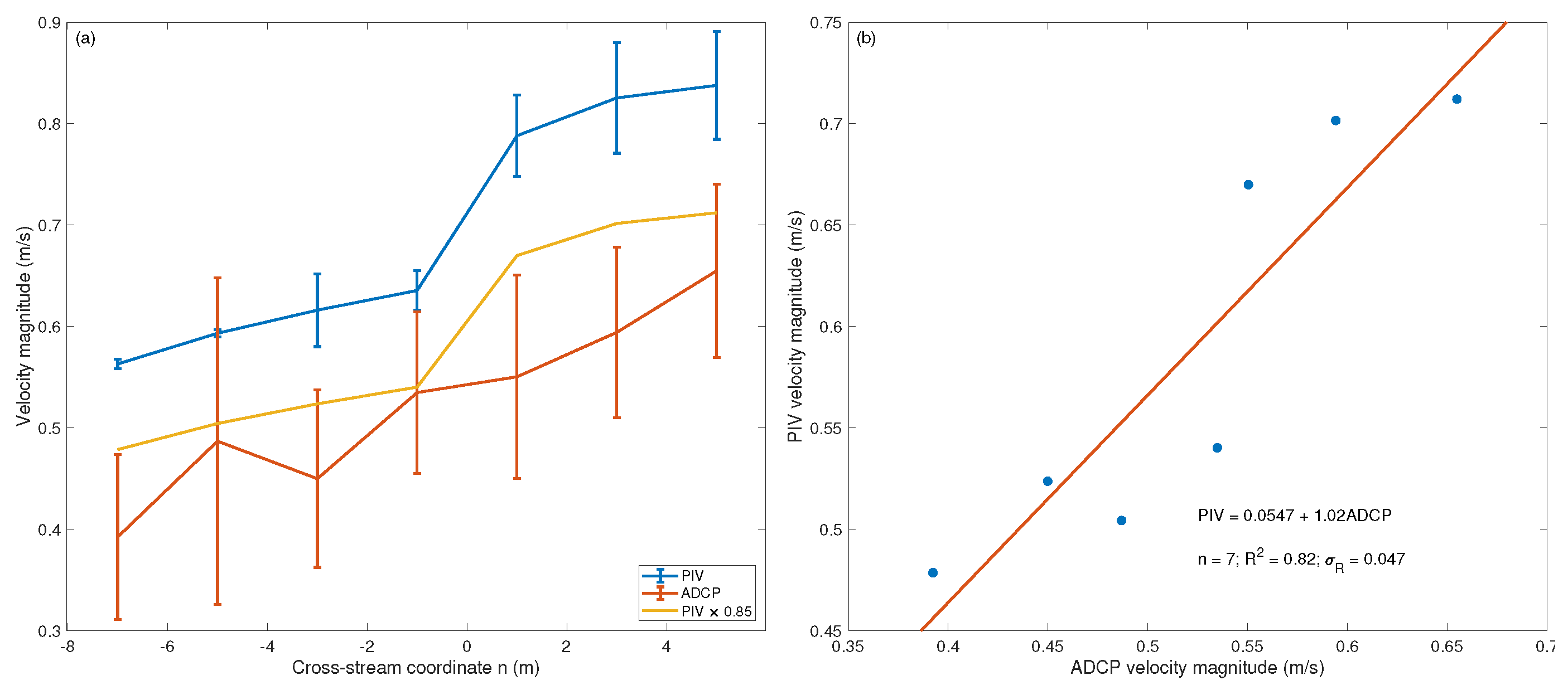
Figure 5a compares the magnitudes of time-averaged thermal PIV surface velocities and depth-averaged ADCP velocities along cross section 1. The error bars represent the total range of velocities within the streamwise extent of the spatial averaging window (at a given cross-stream position) for both the PIV output grid and the four passes made with the ADCP. Lower velocities were observed along the right side (facing downstream) of the channel (negative cross-stream coordinates relative to the channel centerline) and increased to a maximum PIV-based surface velocity of 0.84 m/s. The range of PIV-based surface velocities (i.e., error bars) for a given cross-stream coordinate varied from 0.01 to 0.1 m/s, whereas the ADCP velocities were less precise, with error bars from 0.16 to 0.32 m/s. Adjusting the PIV output with a velocity index of 0.85 brought the depth-averaged velocities from the PIV images within the range of velocities measured directly by the ADCP. Figure 5b quantifies the agreement between the PIV- and ADCP-based depth-averaged velocity magnitudes via linear regression. This analysis resulted in an of 0.82 and a slope approximately equal to 1. The positive intercept implied that, on average, the PIV overestimated the velocity by 0.05 m/s relative to the ADCP.
3.2. Comparison of Lidar-Derived Depths with Field Measurements
The correspondence between the wading, ADCP, and lidar-derived depths is shown in Figure 6a. The ADCP and lidar provided spatially distributed point clouds that were summarized and smoothed by fitting lowess lines to these data sets. The RTK GNSS-based wading measurements were discrete and fewer in number, and the individual points are simply connected by straight lines. All three methodologies captured the asymmetrical shape of cross section 1, with the depth increasing to a maximum of 0.7 m for the wading survey, 0.7 m for the ADCP, and 0.77 m for the lidar. For a given cross-stream location, the lidar-based depths typically varied by 0.10 to 0.12 m within the 1-m swath of data recorded by the ASTRALiTe edge. Because wading provided the simplest and most precise ( m) field-based depth measurements, the RTK GNSS survey was used to evaluate the accuracy of the lidar depths. The results of this analysis are summarized in Figure 6b, which indicates a strong agreement () and a regression line with a slope near one. The intercept term of 0.06 m, however, implied that the lidar overestimated the depth relative to the wading surveys.
3.3. Comparison of Remote Sensing-Based Discharge with Field Measurements
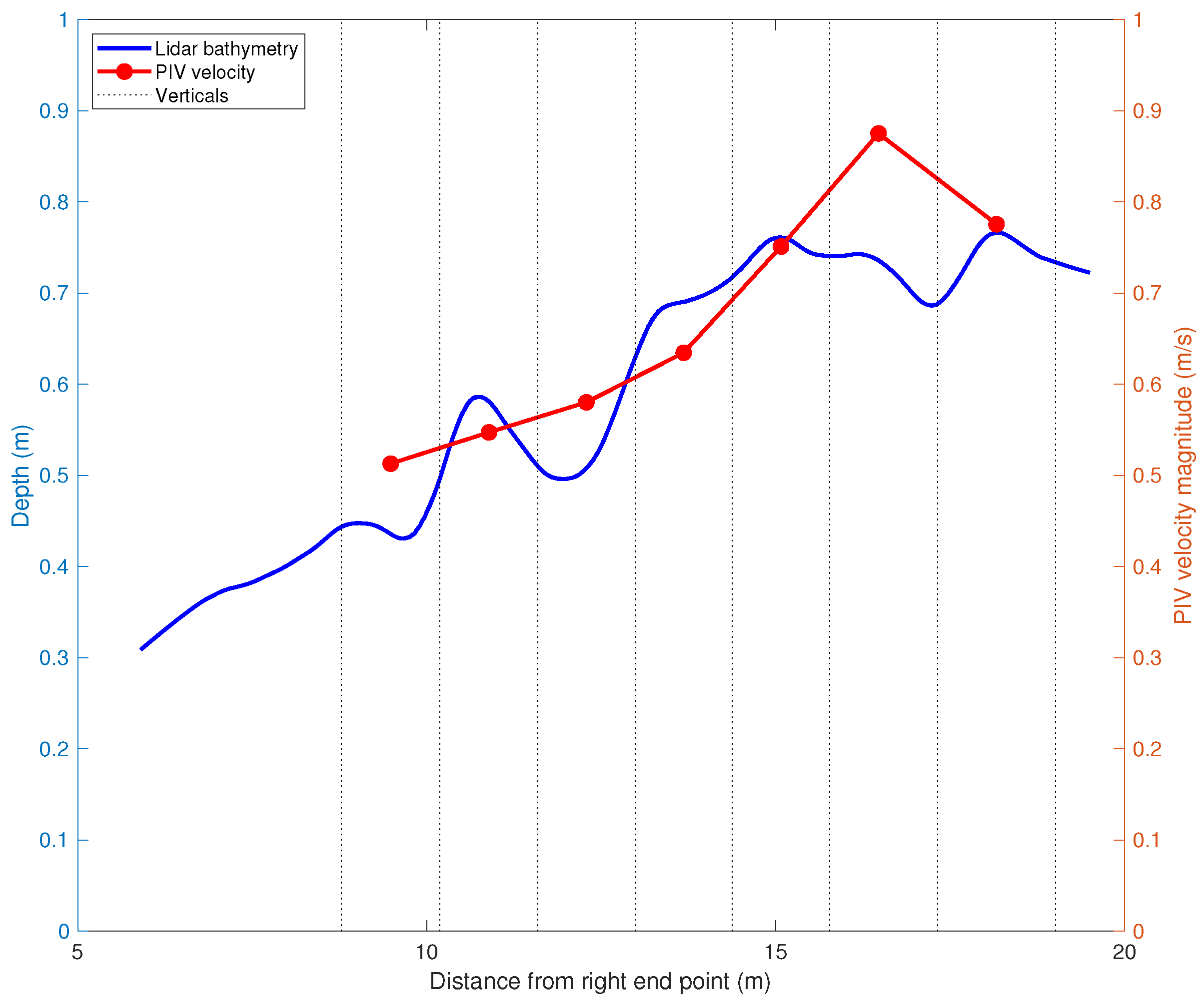
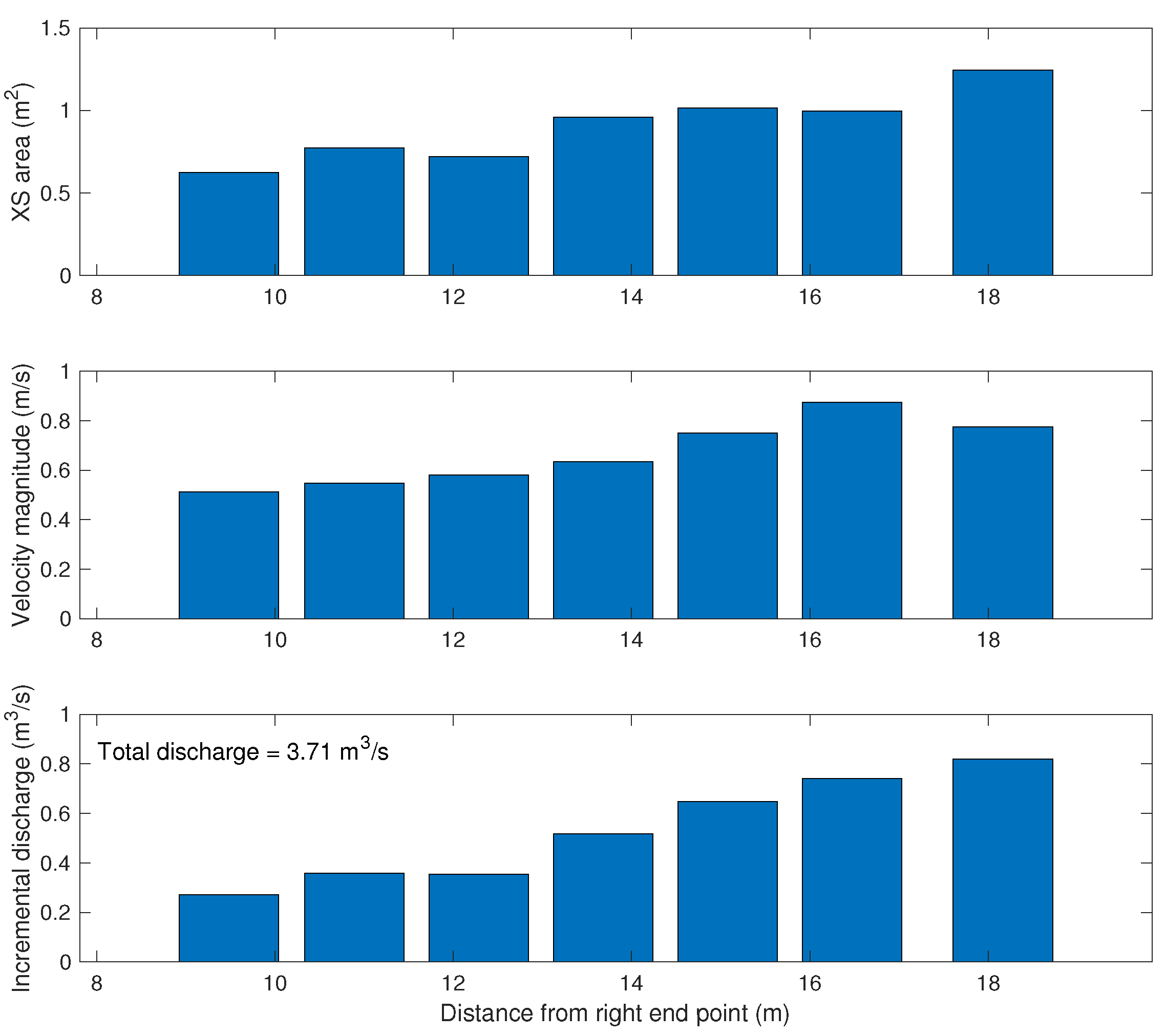
We combined the remotely sensed depths and velocities to calculate the discharge in the Blue River at the time these sUAS-based data sets were acquired. Figure 7 illustrates how both the PIV-derived velocities and lidar-based depths increased from right to left across the channel. Also shown as dashed lines are the left and right edges used to define the width of each vertical used in the incremental discharge calculation. This computation is summarized in Figure 8 for cross section 1. For each of the seven verticals, the cross-sectional area, depth-averaged velocity magnitude, and corresponding incremental discharge are represented by the bar symbols in each panel. Because both depth and velocity increase with distance from the right end point, most of the flow volume within the channel occurred closer to the left bank. Summing the discharge increments laterally across the channel resulted in a total discharge of 3.71 m/s. Applying the same procedure to the subset of the ADCP data that coincided with the lidar coverage resulted in a total discharge of 3.05 m/s. The remote sensing approach thus overestimated the discharge by 22% relative to the ADCP-based calculation for cross section 1. A similar analysis for cross section 2 (see Supplementary Materials Figures S3 and S4) produced much closer agreement, with remote sensing yielding a discharge estimate only 0.16% greater than the ADCP-based value of 6.32 m/s. The discharge for cross section 2 was greater than that for cross section 1 because the lidar was only able to traverse the entire channel width at the second cross section.
4. Discussion
4.1. Potential Sources of Uncertainty in Remotely Sensing of Streamflow
Although various remote sensing technologies could potentially facilitate more efficient, safer measurement of streamflow, the uncertainties inherent to these methods must be acknowledged. Ultimately, our objective was to obtain information on river discharge entirely from remotely sensed data, but this process involved measuring the two fundamental hydraulic quantities that comprise discharge: velocity and depth. In the following subsections, we examine the uncertainties associated with each of these variables in turn and then discuss the implications of these sources of error for discharge calculations.
4.1.1. Uncertainties Associated with Thermal PIV-Based Velocity Estimates
Thermal PIV- and ADCP-based velocities observed along Blue River cross section 1 were compared in Figure 5. For both types of data, the width of the error bars represents the range of velocities present within the spatial-averaging window, providing an indication of measurement precision. The ADCP yielded wider error bars than the PIV because the ADCP data consisted of instantaneous velocity profiles collected as the instrument traversed the channel, whereas the PIV-derived velocities were time-averaged over the one-minute acquisition period. In addition, the ADCP data were collected on four passes that were not exactly coincident with one another and had to be spatially aggregated. The output from the PIV algorithm, in contrast, was a regular grid of velocity vectors with a spacing dictated by the interrogation window and step size parameters we selected. This regular sampling provided a more smoothly varying pattern of cross-stream velocities as well as narrower error bars. Another advantage of PIV is that the method is image-based and produces continuous coverage (i.e., a velocity field) throughout the central portion of an image, not just a single isolated transect (Figure 3). This type of data thus provides greater flexibility in coupling velocity estimates with other data sources, such as bathymetry.
An important limitation of thermal PIV is that this method yields only a surface flow velocity that must somehow be converted to a depth-averaged velocity prior to discharge calculation; this shortcoming pertains to any surface-based velocity measurement technique (e.g., PIV of optical images, radar, GPS-based drifters). Typically, this conversion is achieved by multiplying the surface velocity by a velocity index and this approach brought the PIV-based surface velocities for Blue River cross section 1 to within the error bars of the ADCP data collected along this transect (Figure 5a). We used a value of 0.85, the most common velocity index e.g., [45], but a lower value would have provided better agreement between the PIV- and ADCP-based velocities. Using a velocity index of 0.85 overestimated the depth-averaged velocity in this case, resulting in a positive intercept term for the regression equation in Figure 5b that indicated a positive bias of the PIV-based velocities relative to the ADCP measurements. In general, the velocity index depends on the vertical structure of the flow field and thus varies among rivers and even locally within a reach. For example, Legleiter et al. [22] calculated velocity indices that ranged from 0.82 to 0.93 for five rivers in Alaska. Such variability in the velocity index will introduce a multiplicative error to any surface velocity estimate inferred from remotely sensed data.
4.1.2. Uncertainties Associated with Depths Inferred from Polarized Lidar
Depths measured while wading, by the ADCP and via lidar, were compared in Figure 6. Making this comparison involved determining the best-fit line through the horizontal coordinates of the lidar point cloud and projecting both types of field data onto this line. Although the wading measurements were fewer in number, they were in closer proximity to the lidar transect than the four more irregular passes of the ADCP, which could have contributed to the closer agreement between the lidar-based depths and the wading surveys. Because the wading survey coincided spatially with the lidar swath and consisted of a single transect that did not require spatial averaging, this data source was the most reliable independent check on the accuracy of the lidar-based depths. Relative to the wading data, the ADCP tended to underestimate the depth whereas the lidar was generally biased deep. However, the lidar appears to have captured more subtle features of the bed topography, such as the prominent bump located 12 m from the right end point in Figure 6a.
Another source of uncertainty in comparing the lidar to our field measurements was the nature of the river bed itself. Although the bed was primarily composed of sand and gravel, some submerged aquatic vegetation was also present. Whereas some of the laser pulses might have reflected off the top of the substrate surface (e.g., protruding gravel, vegetation canopy), the survey rod used while wading was more likely to come to rest at lower elevations within the sand, between gravels, or at the base of any plants. One thus might expect the unfiltered lidar point cloud to underestimate the depth relative to the wading survey. For cross section 1 on the Blue River, however, the lidar tended to overestimate the depth. The linear regression used to compare the lidar to the wading depths indicated a strong agreement (), but the intercept term of 0.05 m confirmed the positive bias evident in Figure 6a over the 0.3–0.7 m range of depths sampled along this transect. For cross section 2 (Supplemental Materials Figure S2), the lidar retrieved depths up to 1.2 m but a similar positive intercept of 0.06 m was observed.
Although an explanation for this deep bias is not immediately obvious, one factor that could contribute to this surprising result is the difficulty of identifying the water surface. Lidars do not directly measure the depth but rather calculate the depth as the difference between the range to the water surface and the river bed, as determined from the time of flight of laser pulses returned to the sensor. Any error in establishing the location of the water surface will affect depth estimation because both the refraction of the laser pulse and the change in the speed at which it travels must be accounted for at the air-water interface. The ASTRALiTe polarizing lidar provides an alternative means of distinguishing water surface and bottom returns, which can prove challenging for more common waveform-based bathymetric lidars, particularly in shallow depths where the air-water interface and the stream bed are in such close proximity to one another. However, the initial results presented herein suggest that incorporating polarization information did not enable a completely reliable, binary classification of returns as either water surface or bottom. More specifically, the ASTRALiTe lidar system consists of two channels. The nominal “water-surface channel“ can detect returns from the river bottom when none of the laser pulses experience a specular reflection from the water surface and return to the sensor. This situation is more likely to occur at greater off-nadir angles along the edges of the swath. Similarly, the nominal “bottom surface channel“ can record reflections from the water surface when the specular return from the water surface is strong and overwhelms the optics of the sensor.
4.1.3. Implications for Discharge Calculations
The hydraulic quantities computed from the remotely sensed data and in situ ADCP measurements collected are compared in Table 3. For both cross sections, the mean velocities and cross-sectional areas determined by the remote sensing approach were greater than those calculated from the ADCP measurements. Because each of these components was overestimated when inferred from remotely sensed data, the discharges calculated from thermal PIV and bathymetric lidar exceeded those based on the ADCP data. As shown in Figure 5, even after applying a velocity index of 0.85 thermal PIV overestimated the corresponding ADCP-derived depth-averaged velocity, which in turn lead to overestimation of the discharge. Similarly, the deep bias observed for the lidar bathymetry (Figure 6) yielded greater cross-sectional areas than the field surveys and also contributed to the overestimation of discharge. In general, an overprediction of the mean velocity from remotely sensed data could be compensated for by an underprediction of the cross-sectional area or vice versa, but for both of the cross sections sampled on the Blue River overestimation of both hydraulic quantities ensured that the total discharge would be overpredicted relative to the field measurements.
A notable feature of Table 3 is that the discharges calculated for the two cross sections, which were located in close proximity to one another, differed by 2.62 m/s for the remote sensing approach and by 3.27 m/s for the ADCP-based calculation. In addition, the agreement between the remote sensing and field-based discharges was much better for cross section 2, with only a 0.1% discrepancy at this transect, whereas the discharge was overestimated by the remotely sensed data by 22% at the upstream transect. These differences between the two cross sections are primarily a consequence of the greater coverage achieved by the lidar at cross section 2, where the sUAS was able to safely traverse the entire channel width. Vegetation along the left bank at cross section 1 prevented the sUAS from sampling the left side of the channel and restricted our discharge calculation to only a portion of the width. Because most of the flow through this reach of the Blue River was concentrated along the left side of the channel, a lack of data from this area precluded us from calculating an accurate total discharge for cross section 1. For the other transect, more complete coverage resulted in a calculated discharge closer to the value of approximately 6 m/s recorded at the upstream USGS gaging station (09057500 Blue River below Green Mountain Reservoir, CO).
4.2. Practical Considerations for Remotely Sensing of River Discharge
This initial pilot study revealed a number of factors that must be considered carefully in any application of an sUAS-based remote sensing approach to measuring river discharge. In this section, we discuss some of the practical lessons we learned to help guide future work based on the methodology described herein. We describe both instrumentation-related issues and operational restrictions that must be taken into account during mission planning.
Through several previous attempts to infer surface flow velocities from thermal image time series, we learned that suitable image data can only be acquired under certain environmental conditions. The thermal features tracked by the PIV algorithm are most pronounced when the temperature contrast between the water and the overlying air is greatest. This is most likely to occur at dawn when the air has cooled more overnight than the water, which has a much higher specific heat capacity. During the day, the air and water temperatures tend to converge, obscuring the water-surface thermal features of interest. In addition, reflected solar energy can become a significant fraction of the radiation recorded by the thermal camera when the sun is higher in the sky. Another way to enhance the detection of subtle differences in temperature is to use a cooled mid-wave infrared thermal camera. This type of sensor has a greater sensitivity, typically with a noise equivalent temperature difference <0.025 °C, and thus provides better clarity and contrast than more readily available uncooled thermal cameras. However, disadvantages of cooled thermal cameras include greater cost, larger size, and susceptibility to reflections from the sun [48]. Pixel size, frame acquisition rate, data capture rate, and on-board data storage capacity are also important criteria to evaluate in selecting an appropriate thermal camera.
Although this was the initial field test of the sUAS-based ASTRALiTe edge lidar in a river, we can make some general statements about the use of this technology for measuring river bathymetry. As with airborne lidar, water clarity is an important constraint on the ability of laser pulses to penetrate through the water column to the stream bed. Substrate reflectivity can also limit the number of bottom returns. While a more powerful laser might help to overcome these obstacles, greater power would likely come at the expense of a heavier payload that would not be conducive to sUAS deployments. Regulations that ensure eye safety also constrain the amount of laser power a lidar system can use. In this study, flying the ASTRALiTe edge 4 m above the water surface provided a high density of bottom returns in a clear-flowing channel up to 1.2 m deep. However, this low flying height limited the coverage that could be achieved because riparian vegetation presented a hazard to the sUAS. In designing and deploying a bathymetric lidar system, a safe compromise must be reached between at least three principal factors: (1) laser power and penetration depth, (2) system weight and flight duration, and (3) flying height and obstacle avoidance.
In addition to these instrumentation-related issues, regulatory restrictions also can limit the suitability of sUAS-based remotely sensed data for characterizing streamflow. Ideally, an sUAS would be flown high enough for the imaging system to capture not only the entire channel width but also at least a small area along the banks so that targets placed to provide ground control are visible. In this study, however, a small local airport with one runway located 2 km from our study area dictated a maximum flight altitude of 100 m, per Federal Aviation Administration (FAA) regulations. As a result, the channel and both banks were only included in a single image for one of the two cross sections. For the second, wider transect, two separate hovering waypoints were required to image both banks, which was necessary because spatially distributed ground control is needed to accurately scale and geo-reference the images and the velocity vectors derived therefrom. For cross section 2, the lack of targets on both sides of the images complicated geo-referencing and we used images acquired from only one of the two waypoints for PIV and discharge calculation. At this location, the vast majority of the flow was captured by images of the left side of the channel. Images from the right side encompassed a broad shallow area dominated by submerged vegetation that conveyed a negligible portion of the total river discharge. This local configuration allowed us to derive a reasonable discharge estimate from an image sequence that did not span the entire channel width, but this will not be the case in general. More typically, restrictions on flying height could dictate that partial discharges derived from multiple image sequences distributed laterally across the channel be combined to obtain the total discharge.
4.3. Future Research Directions
This pilot study served as an initial test of the feasibility of measuring river discharge via sUAS-based remote sensing and also highlighted some important topics for further investigation. In this section, we discuss some potential refinements to instrumentation and make suggestions to improve data collection and processing.
Although the sensors used in this study fulfilled their intended purpose, both the thermal camera and polarizing lidar system will require further development and testing before this approach can become more broadly applicable. For example, the frame acquisition and data capture rate of the thermal camera was limited to a relatively low 0.5 Hz, much less than the 25–30 Hz frame rates typically used in LSPIV applications based on conventional video cameras. In this case study, the low frame rate did not compromise PIV due to the relatively low surface flow velocities observed along the Blue River at a base flow discharge in late fall but could prove to be problematic at higher discharges and/or in more energetic channels. Similarly, the sensitivity of the lidar to various environmental conditions must be examined through additional field tests. Whereas the water surface of the Blue River was very smooth at the time of this study, rougher water surface textures could affect the interaction of laser pulses with the air-water interface and thus reduce the accuracy of lidar-derived bathymetric information. The Blue River also was relatively clear at the time of our survey, but the lidar system would not be expected to perform as well in more turbid water. Our study site only included depths up to 1.2 m, so further testing in deeper rivers is needed to quantify the maximum penetration depth of the ASTRALiTe edge. In the initial field evaluation described herein, the thermal camera and the lidar were deployed independently on separate sUAS, but in the future this instrumentation package could be deployed from a single sUAS platform. However, such consolidation would increase the weight of the payload and reduce flight duration and thus would only be beneficial if both sensors could acquire useful data from the same flying height.
Improvements to the data collection and processing we performed in this study could help remote sensing to become a viable operational tool for measuring river discharge. For example, in future field evaluations a cable (i.e., tagline) should be stretched across the channel for two reasons. First, the tagline would provide a clear linear feature that the pilot could use for guidance while operating the sUAS manually, rather than relying upon pre-programmed waypoints and automated navigation. Second, the tagline would facilitate collection of in situ velocity verification data by guiding the ADCP along a straight transect coincident with the lidar swath, rather than the irregular passes that we recorded in this study. Another, more general issue that requires further research is the selection of an appropriate velocity index to convert PIV-based surface velocities to depth-averaged velocities prior to calculating discharge. In this study we scaled and geo-referenced the thermal images based on ground control targets placed in the field, but a more efficient alternative would be direct geo-referencing of the images using position and orientation data logged on-board the sUAS; this approach would obviate the need to place ground control targets along the banks and/or in the river. If absolute spatial coordinates are not necessary for a given application, only the scale factor for converting pixels to meters is needed to perform PIV. This scale could be established by using a laser range finder or ultrasonic sensor to measure the distance from the sUAS down to the water surface and calculating the ground sampling distance based on the focal length of the camera. Finally, although the current workflow would require a hydrographer to collect data in the field and then post-process the images and analyze the lidar before performing a discharge computation, this workflow could be streamlined if some of this processing (i.e., PIV) could be performed in real-time on-board the sUAS, on the sensor directly, or processed on the ground control station system. Performing the data processing outside of the sUAS increases portability by keeping the sensor independent of the platform, thus providing the greatest flexibility for deployment. In addition, further development of the lidar processing algorithms could allow the point cloud to be visualized by an operator on the ground. This type of real-time feedback would help to ensure that remote sensing-based measurements of velocity and depth are of sufficient quality.
5. Conclusions
Remote sensing offers the potential to improve the safety of the hydrographer and increase the efficiency of on-site streamflow measurements. These advances would also allow the USGS and similar agencies worldwide to expand their hydrologic monitoring networks into remote, inaccessible locations and ungaged basins. Recent technological developments have reduced the size, weight, and power consumption of sensors to a degree that instrumentation that previously could only be carried on conventional occupied aircraft now can be deployed from sUAS platforms. In this paper, we describe a complete technique for collecting both the surface flow velocity and bathymetric data necessary to compute river discharge from an sUAS under natural conditions. This approach involved the use of a thermal infrared camera, a PIV algorithm, and a polarizing lidar. Importantly, the sensors, platforms, and software used in this study are all commercially available at this time, not just prototypes in an early stage of development.
We evaluated the performance of this approach by comparing remotely sensed velocities and depths to field measurements collected at two cross sections along the Blue River, CO, USA. The results of this investigation support the following principal conclusions:
- Compact, sUAS-deployable thermal infrared cameras of sufficient sensitivity can detect the movement of flow features expressed at the water surface as subtle differences in temperature, thus enabling PIV without requiring visible tracer materials or artificial seeding of the flow.
- Incorporating information on the polarization of returned laser pulses provides an alternative means of distinguishing the water surface from the channel bed even in very shallow water; these polarizing lidar systems also are small enough to be deployed from an sUAS.
- Due to limited payload capacity and differences in flying height during data collection, the thermal camera and polarizing lidar had to be deployed from separate sUAS.
- Surface flow velocities inferred from thermal images via PIV agreed closely ( = 0.82 and 0.64) with depth-averaged flow velocities measured in situ with an ADCP when multiplied by the commonly assumed velocity index of 0.85.
- Depths derived from the polarizing lidar closely matched those surveyed by wading in the shallower of the two cross sections ( = 0.95), but the agreement was not as strong for the transect with greater depths ( = 0.61), although the sensor was able to detect the bottom in depths up to 1.2 m.
- These remotely sensed velocities and depths were combined to calculate incremental discharges that were summed laterally across the channel to obtain the total streamflow. As compared with discharges calculated in a similar manner directly from the ADCP data, the sUAS-based methodology resulted in a discharge that was 22% greater at one cross section but within 0.1% of the ADCP-based discharge at the second cross section.
Supplementary Materials
The following are available online at https://www.mdpi.com/2072-4292/11/19/2317/s1.
Author Contributions
Conceptualization, P.J.K., C.J.L.; methodology, P.J.K., C.J.L.; software, C.J.L., P.J.K.; validation, P.J.K., C.J.L.; resources, P.J.K., C.J.L.; writing—original draft preparation, P.J.K., C.J.L.; writing—review and editing, P.J.K., C.J.L.; visualization, C.J.L., P.J.K.; project administration, P.J.K., C.J.L.
Funding
This research was supported by the U.S. Geological Survey’s Water Mission Area Hydrologic Remote Sensing Branch and the U.S. Geological Survey’s National Unmanned Aircraft Systems Project Office.
Acknowledgments
Jonathan Nelson, Yutaka Higashi, Jeff Sloan, Jack Eggleston, and Cian Dawson (USGS); Cotton Anderson, Bill Adams, and Gerald Thompson (ASTRALiTe); Jeffery Thayer, Rory Barton-Grimley, Toby Minear, and Brian Straight (University of Colorado at Boulder); David White, Jack Davis, and Evan Menke (Juniper Unmanned). The field measurements and image data sets used in this study are available through the USGS ScienceBase Catalog data release listed in the references. Any use of trade, firm, or product names is for descriptive purposes only and does not imply endorsement by the U.S. Government.
Conflicts of Interest
The authors declare no conflict of interest.
References
- Eberts, S.; Woodside, M.; Landers, M.; Wagner, C. Monitoring the pulse of our Nation’s rivers and streams—The U.S. Geological Survey streamgaging network. U.S. Geol. Surv. Fact Sheet 2018-3021 2018. [Google Scholar] [CrossRef]
- Gordon, R.L. Acoustic Measurement of River Discharge. J. Hydraul. Eng. 1989, 115, 925–936. [Google Scholar] [CrossRef]
- Simpson, M.R.; Oltmann, R.N. Discharge-measurement system using an acoustic Doppler current profiler with applications to large rivers and estuaries. USGS Water Supply Pap. 2395 1993, 32. [Google Scholar] [CrossRef]
- Oberg, K.A.; Morlock, S.E.; Caldwell, W.S. Quality assurance plan for discharge measurements using acoustic Doppler current profilers. U.S. Geol. Surv. Sci. Investig. Rep. 5135 2005, 35. [Google Scholar] [CrossRef]
- Mueller, D.S. Extrap: Software to assist the selection of extrapolation methods for moving-boat ADCP streamflow measurements. Comput. Geosci. 2013, 54, 211–218. [Google Scholar] [CrossRef]
- Turnipseed, D.; Sauer, V. Discharge measurements at gaging stations. U.S. Geol. Surv. Tech. Methods Book 3 2010, 87. [Google Scholar] [CrossRef]
- Fujita, I.; Komura, S. Application of Video Image Analysis for Measurements of River-Surface Flows. Proc. Hydraul. Eng. JSCE 1994, 38, 733–738. [Google Scholar] [CrossRef]
- Lin, D.; Grundmann, J.; Eltner, A. Evaluating Image Tracking Approaches for Surface Velocimetry With Thermal Tracers. Water Resour. Res. 2019, 55, 3122–3136. [Google Scholar] [CrossRef]
- Dugan, J.P.; Anderson, S.P.; Piotrowski, C.C.; Zuckerman, S.B. Airborne Infrared Remote Sensing of Riverine Currents. IEEE Trans. Geosci. Remote. Sens. 2014, 52, 3895–3907. [Google Scholar] [CrossRef]
- Altenau, E.H.; Pavelsky, T.M.; Moller, D.; Lion, C.; Pitcher, L.H.; Allen, G.H.; Bates, P.D.; Calmant, S.; Durand, M.; Smith, L.C. AirSWOT measurements of river water surface elevation and slope: Tanana River, AK. Geophys. Res. Lett. 2017, 44, 181–189. [Google Scholar] [CrossRef] [Green Version]
- Tauro, F.; Pagano, C.; Phamduy, P.; Grimaldi, S.; Porfiri, M. Large-Scale Particle Image Velocimetry From an Unmanned Aerial Vehicle. IEEE/ASME Trans. Mechatronics 2015, 20, 3269–3275. [Google Scholar] [CrossRef]
- Tauro, F.; Porfiri, M.; Grimaldi, S. Surface flow measurements from drones. J. Hydrol. 2016, 540, 240–245. [Google Scholar] [CrossRef] [Green Version]
- Bandini, F.; Olesen, D.; Jakobsen, J.; Kittel, C.M.M.; Wang, S.; Garcia, M.; Bauer-Gottwein, P. Technical note: Bathymetry observations of inland water bodies using a tethered single-beam sonar controlled by an unmanned aerial vehicle. Hydrol. Earth Syst. Sci. 2018, 22, 4165–4181. [Google Scholar] [CrossRef] [Green Version]
- Gleason, C.J.; Smith, L.C. Toward global mapping of river discharge using satellite images and at-many-stations hydraulic geometry. Proc. Natl. Acad. Sci. USA 2014, 111, 4788–4791. [Google Scholar] [CrossRef] [PubMed] [Green Version]
- Bjerklie, D.M.; Birkett, C.M.; Jones, J.W.; Carabajal, C.; Rover, J.A.; Fulton, J.W.; Garambois, P.A. Satellite remote sensing estimation of river discharge: Application to the Yukon River, Alaska. J. Hydrol. 2018, 561, 1000–1018. [Google Scholar] [CrossRef]
- Muste, M.; Fujita, I.; Hauet, A. Large-scale particle image velocimetry for measurements in riverine environments. Water Resour. Res. 2008, 44. [Google Scholar] [CrossRef] [Green Version]
- Perks, M.T.; Russell, A.J.; Large, A.R.G. Technical Note: Advances in flash flood monitoring using unmanned aerial vehicles (UAVs). Hydrol. Earth Syst. Sci. 2016, 20, 4005–4015. [Google Scholar] [CrossRef] [Green Version]
- Tauro, F.; Tosi, F.; Mattoccia, S.; Toth, E.; Piscopia, R.; Grimaldi, S. Optical Tracking Velocimetry (OTV): Leveraging Optical Flow and Trajectory-Based Filtering for Surface Streamflow Observations. Remote. Sens. 2018, 10, 2010. [Google Scholar] [CrossRef]
- Dugdale, S.J. A practitioner’s guide to thermal infrared remote sensing of rivers and streams: Recent advances, precautions and considerations. Wiley Interdiscip. Rev. Water 2016, 3, 251–268. [Google Scholar] [CrossRef]
- Chickadel, C.C.; Horner-Devine, A.R.; Talke, S.A.; Jessup, A.T. Vertical boil propagation from a submerged estuarine sill. Geophys. Res. Lett. 2009, 36. [Google Scholar] [CrossRef] [Green Version]
- Puleo, J.A.; McKenna, T.E.; Holland, K.T.; Calantoni, J. Quantifying riverine surface currents from time sequences of thermal infrared imagery. Water Resour. Res. 2012, 48. [Google Scholar] [CrossRef] [Green Version]
- Legleiter, C.J.; Kinzel, P.J.; Nelson, J.M. Remote measurement of river discharge using thermal particle image velocimetry (PIV) and various sources of bathymetric information. J. Hydrol. 2017, 554, 490–506. [Google Scholar] [CrossRef]
- Gilvear, D.J.; Waters, T.M.; Milner, A.M. Image analysis of aerial photography to quantify changes in channel morphology and instream habitat following placer mining in interior Alaska. Freshw. Biol. 1995, 34, 389–398. [Google Scholar] [CrossRef]
- Legleiter, C.J.; Roberts, D.A.; Lawrence, R.L. Spectrally based remote sensing of river bathymetry. Earth Surf. Process. Landforms 2009, 34, 1039–1059. [Google Scholar] [CrossRef]
- Westaway, R.M.; Lane, S.N.; Hicks, D.M. The development of an automated correction procedure for digital photogrammetry for the study of wide, shallow, gravel-bed rivers. Earth Surf. Process. Landforms 2000, 25, 209–226. [Google Scholar] [CrossRef]
- Dietrich, J.T. Bathymetric Structure-from-Motion: Extracting shallow stream bathymetry from multi-view stereo photogrammetry. Earth Surf. Process. Landforms 2017, 42, 355–364. [Google Scholar] [CrossRef]
- Kasvi, E.; Salmela, J.; Lotsari, E.; Kumpula, T.; Lane, S. Comparison of remote sensing based approaches for mapping bathymetry of shallow, clear water rivers. Geomorphology 2019, 333, 180–197. [Google Scholar] [CrossRef]
- Legleiter, C.J. Calibrating remotely sensed river bathymetry in the absence of field measurements: Flow REsistance Equation-Based Imaging of River Depths (FREEBIRD). Water Resour. Res. 2015, 51, 2865–2884. [Google Scholar] [CrossRef]
- Legleiter, C.J. Inferring river bathymetry via Image-to-Depth Quantile Transformation (IDQT). Water Resour. Res. 2016, 52, 3722–3741. [Google Scholar] [CrossRef] [Green Version]
- Guenther, G.; Cunningham, A.; LaRoque, P.; Reid, D. Meeting the accuracy challenge in airborne lidar bathymetry. In Proceedings of the 20th EARSeL Symposium: Workshop on LiDAR Remote Sensing of Land and Sea, Dresden, Germany, 16–17 June 2000. [Google Scholar]
- Kinzel, P.J.; Wright, C.W.; Nelson, J.M.; Burman, A.R. Evaluation of an Experimental LiDAR for Surveying a Shallow, Braided, Sand-Bedded River. J. Hydraul. Eng. 2007, 133, 838–842. [Google Scholar] [CrossRef] [Green Version]
- Hilldale, R.C.; Raff, D. Assessing the ability of airborne LiDAR to map river bathymetry. Earth Surf. Process. Landforms 2008, 33, 773–783. [Google Scholar] [CrossRef]
- Kinzel, P.J.; Legleiter, C.J.; Nelson, J.M. Mapping river bathymetry with a small footprint green LiDAR: Applications and challenges. J. Am. Water Resour. Assoc. 2013, 49, 183–204. [Google Scholar] [CrossRef]
- Mandlburger, G.; Pfennigbauer, M.; Wieser, M.; Riegl, U.; Pfeifer, N. Evaluation of a novel uav-borne topo-bathymetric laser profiler. Int. Arch. Photogramm. Remote. Sens. Spat. Inf. Sci. 2016, XLI-B1, 933–939. [Google Scholar] [CrossRef]
- Legleiter, C.J.; Overstreet, B.T.; Glennie, C.L.; Pan, Z.; Fernandez-Diaz, J.C.; Singhania, A. Evaluating the capabilities of the CASI hyperspectral imaging system and Aquarius bathymetric LiDAR for measuring channel morphology in two distinct river environments. Earth Surf. Process. Landforms 2016, 41, 344–363. [Google Scholar] [CrossRef]
- Spicer, K.R.; Costa, J.E.; Placzek, G. Measuring flood discharge in unstable stream channels using ground-penetrating radar. Geology 1997, 25, 423. [Google Scholar] [CrossRef]
- Costa, J.E.; Spicer, K.R.; Cheng, R.T.; Haeni, F.P.; Melcher, N.B.; Thurman, E.M.; Plant, W.J.; Keller, W.C. Measuring stream discharge by non-contact methods: A Proof-of-Concept Experiment. Geophys. Res. Lett. 2000, 27, 553–556. [Google Scholar] [CrossRef]
- Melcher, N.B.; Thurman, E.M.; Buursink, M.; Spicer, K.R.; Hayes, E.; Plant, W.J.; Keller, W.C.; Hayes, K.; Costa, J.E.; Haeni, F.P.; et al. River discharge measurements by using helicopter-mounted radar. Geophys. Res. Lett. 2002, 29, 41–44. [Google Scholar] [CrossRef]
- Legleiter, C.J.; Kinzel, P.J. UAS-based remotely sensed data and field measurements of flow depth and velocity from the Blue River, Colorado, October 18, 2018. U.S. Geol. Surv. Data Release 2019. [Google Scholar] [CrossRef]
- Thielicke, W.; Stamhuis, E.J. PIVlab—Towards User-friendly, Affordable and Accurate Digital Particle Image Velocimetry in MATLAB. J. Open Res. Softw. 2014, 2, e30. [Google Scholar] [CrossRef]
- Thielicke, W. The Flapping Flight of Birds—Analysis and Application. Ph.D. Thesis, Rijksuniversiteit Groningen, Groningen, The Netherlands, 2014. [Google Scholar]
- Thielicke, W.; Stamhuis, E.J. PIVlab—Time-Resolved Digital Particle Image Velocimetry Tool for MATLAB (version: 1.43). Available online: http://dx.doi.org/10.6084/m9.figshare.1092508 (accessed on 29 April 2019).
- Mitchell, S.; Thayer, J.P.; Hayman, M. Polarization lidar for shallow water depth measurement. Appl. Opt. 2010, 49, 6995–7000. [Google Scholar] [CrossRef]
- Mitchell, S.E.; Thayer, J.P. Ranging through Shallow Semitransparent Media with Polarization Lidar. J. Atmos. Ocean. Technol. 2014, 31, 681–697. [Google Scholar] [CrossRef]
- Rantz, S.; Others, A. Measurement and Computation of Streamflow: Volume 1. Measurement of Stage and Discharge. U.S. Geol. Surv. Water Supply Pap. 1982, 2175, 284. [Google Scholar] [CrossRef]
- Helsel, D.R.; Hirsch, R.M. Statistical Methods in Water Resources (Techniques of Water-Resources Investigations of the United States Geological Survey, Book 4, Hydrologic Analysis and Interpretation, Chapter A3). U.S. Geol. Surv. 2002, 1–524. [Google Scholar] [CrossRef]
- Dilbone, E.; Legleiter, C.J.; Alexander, J.S.; McElroy, B. Spectrally based bathymetric mapping of a dynamic, sand-bedded channel: Niobrara River, Nebraska, USA. River Res. Appl. 2018, 34, 430–441. [Google Scholar] [CrossRef]
- Gade, R.; Moeslund, T.B. Thermal cameras and applications: A survey. Mach. Vis. Appl. 2014, 25, 245–262. [Google Scholar] [CrossRef]
Figure 1.
Location of study area and the two cross sections on the Blue River where discharge calculations were made. The edge of water, a shallow submerged bar, and the positions of the weather station and thermistor are also shown.
Figure 1.
Location of study area and the two cross sections on the Blue River where discharge calculations were made. The edge of water, a shallow submerged bar, and the positions of the weather station and thermistor are also shown.

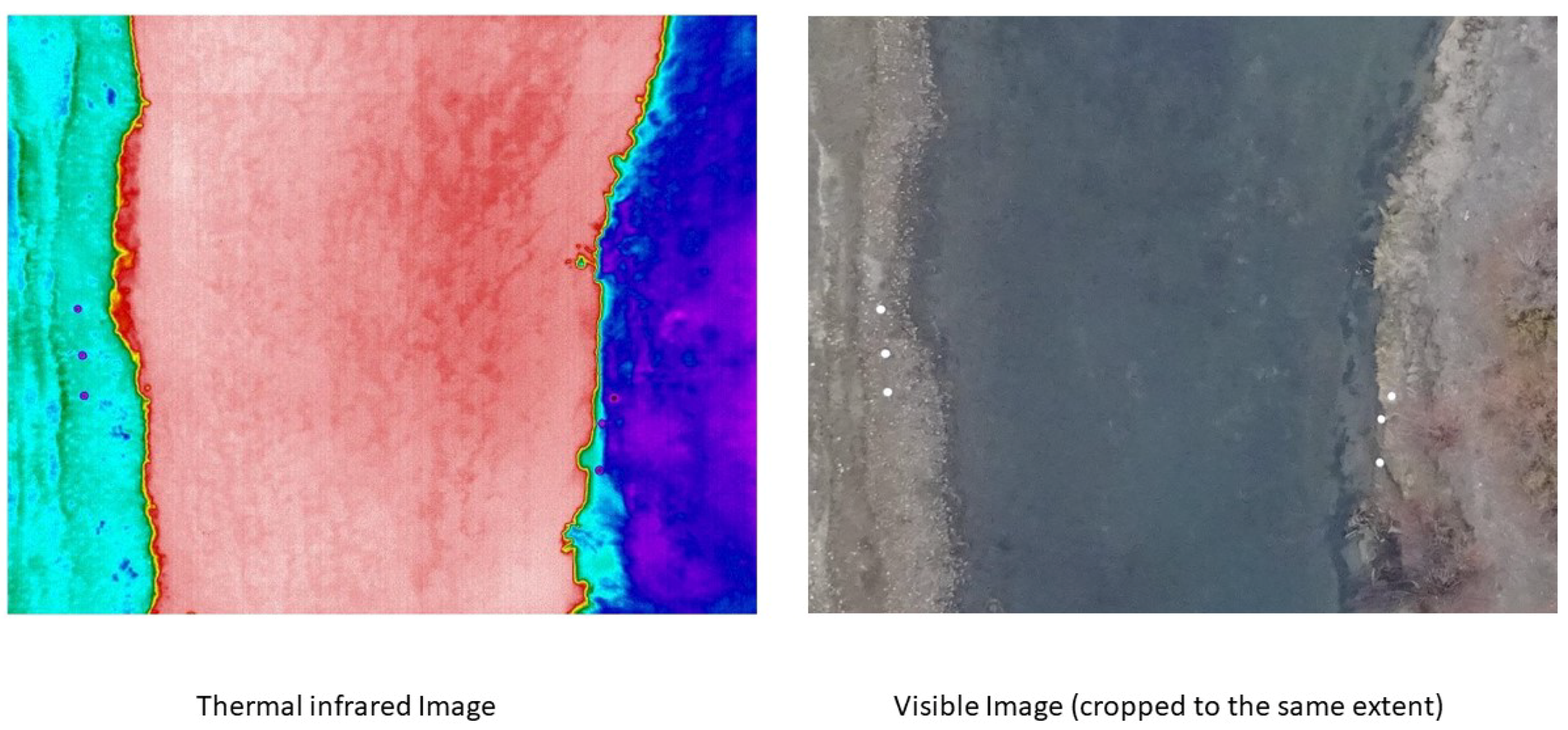
Figure 2.
Imagery collected by sUAS camera platform over cross section 1. The aluminum disks used as ground control points appear as dark purple circular features in the thermal image and as white circles in the visible image.
Figure 2.
Imagery collected by sUAS camera platform over cross section 1. The aluminum disks used as ground control points appear as dark purple circular features in the thermal image and as white circles in the visible image.

Figure 3.
PIV-derived velocity vectors for cross section 1.

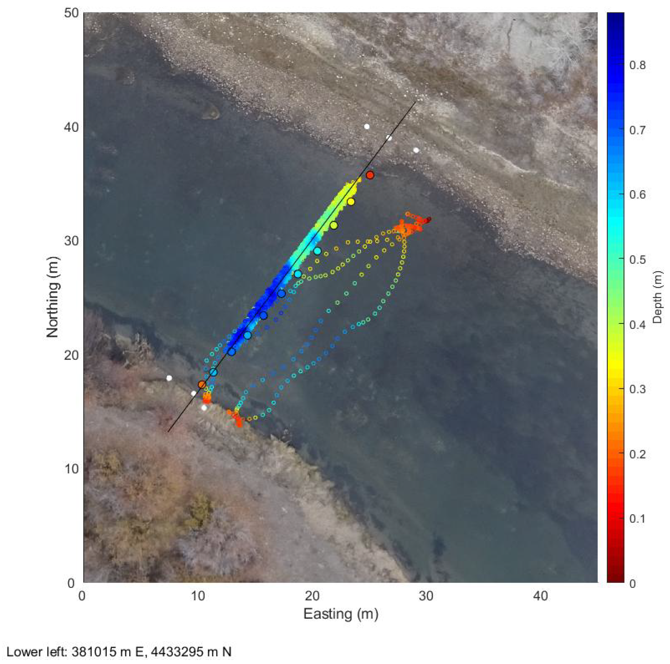
Figure 4.
Depths measured by wading (large filled symbols with black circle outlines), ADCP (mid-size open symbols with colored circle outlines), and lidar (small filled symbols) collected at cross section 1.
Figure 4.
Depths measured by wading (large filled symbols with black circle outlines), ADCP (mid-size open symbols with colored circle outlines), and lidar (small filled symbols) collected at cross section 1.

Figure 5.
(a) Comparison of PIV-derived velocities and ADCP measurements along cross section 1. (b) Accuracy assessment of PIV-derived depth-averaged velocities via linear regression.
Figure 5.
(a) Comparison of PIV-derived velocities and ADCP measurements along cross section 1. (b) Accuracy assessment of PIV-derived depth-averaged velocities via linear regression.

Figure 6.
(a) Depth comparison between lidar, wading, and ADCP measurements along cross section 1. (b) Accuracy assessment of lidar-derived depths via linear regression.
Figure 6.
(a) Depth comparison between lidar, wading, and ADCP measurements along cross section 1. (b) Accuracy assessment of lidar-derived depths via linear regression.

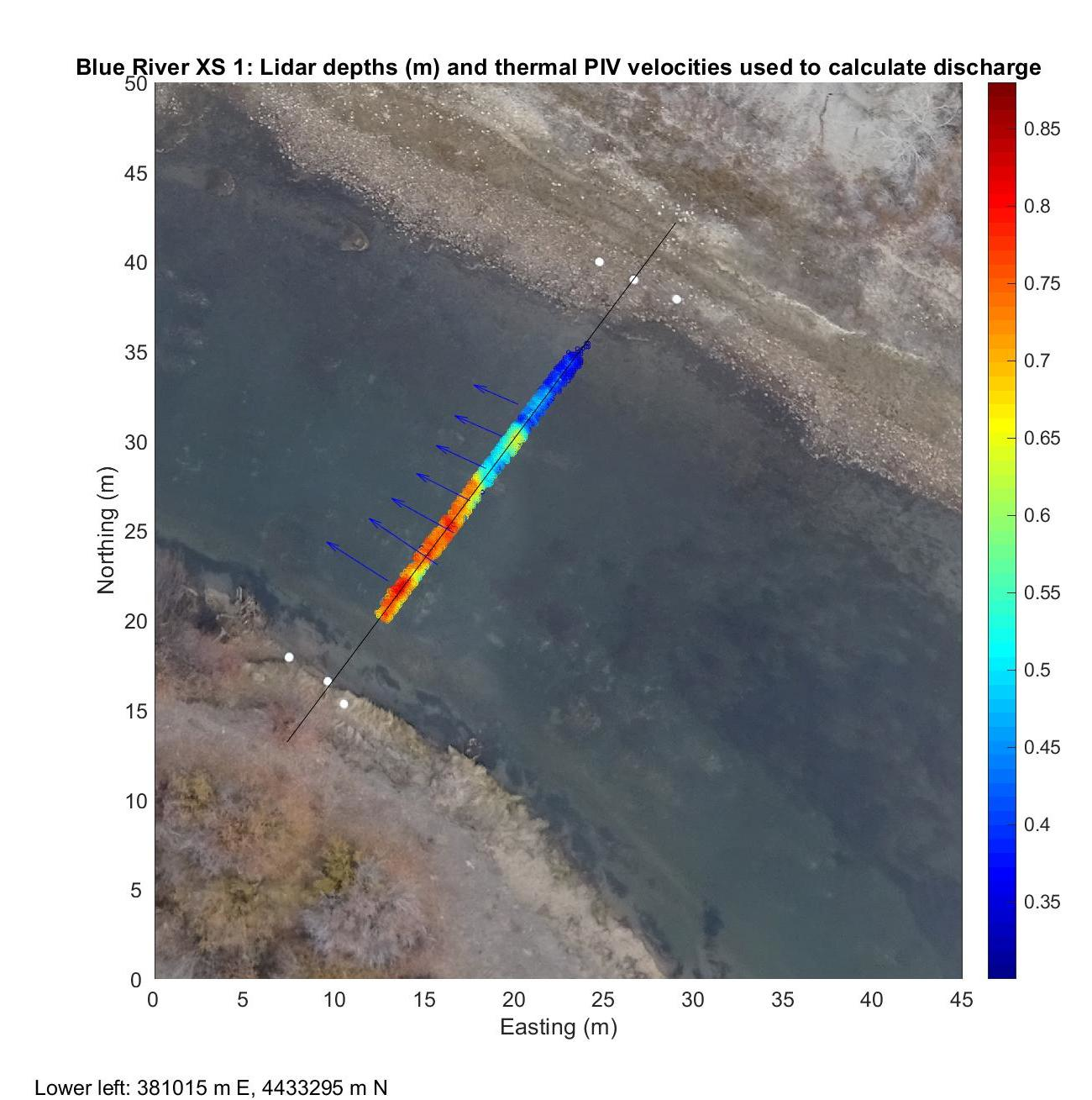
Figure 7.
PIV-derived velocities, lidar depths, and left and right edges for each vertical used in the incremental discharge calculation for cross section 1 based entirely on remotely sensed data.
Figure 7.
PIV-derived velocities, lidar depths, and left and right edges for each vertical used in the incremental discharge calculation for cross section 1 based entirely on remotely sensed data.

Figure 8.
Illustration of how the cross sectional area associated with each vertical is multiplied by the corresponding velocity magnitude to yield a series of incremental discharges that are then summed laterally to obtain the total discharge. This example is based on remotely sensed data from cross section 1 on the Blue River.


Table 1.
Specifications of small Unmanned Aerial System (sUAS) thermal camera.
| Model | ICI Mirage 640 |
|---|---|
| Lens | 25 mm lens (26° field of view) |
| Detector | Cooled Indium Antimonide |
| Pixel dimensions on focal array | 15 m |
| Number of pixels | 640 × 512 |
| Wavelength range | 3.4 m–5.1 m |
| Noise-equivalent temperature difference | <0.012 °C at 30 °C |
| Bits per pixel | 14 |
| Camera dimensions | 111 × 96 × 131 mm |
| Camera weight | 765 g |
| Power | 12 V |
Table 2.
Specifications of small Unmanned Aerial System (sUAS) bathymetric lidar.
| Model | ASTRALiTe edge |
|---|---|
| Laser Wavelength | 532 nm |
| Laser Power | 30 mW |
| Swath Width | 1/2 flight altitude |
| Depth Penetration | Secchi depth |
| Scan Technique | Whisk broom |
| Positioning | SBG Ellipse2-D INS |
| Weight | 5 kg |
| Dimensions | 0.18 m × 0.2 m × 0.23 m |
| Flight Duration | 10–12 min on DJI Matrice 600 Pro |
Table 3.
Hydraulic quantities calculated from remotely sensed data and field-based ADCP measurements for two cross sections on the Blue River.
Table 3.
Hydraulic quantities calculated from remotely sensed data and field-based ADCP measurements for two cross sections on the Blue River.
| Quantity | Cross Section | Remote sensing | ADCP |
|---|---|---|---|
| Mean velocity (m/s) | 1 | 0.67 | 0.58 |
| 2 | 0.42 | 0.36 | |
| cross sectional area (m) | 1 | 6.33 | 5.06 |
| 2 | 16.31 | 14.10 | |
| Total discharge (m/s) | 1 | 3.71 | 3.05 |
| 2 | 6.33 | 6.32 |
© 2019 by the authors. Licensee MDPI, Basel, Switzerland. This article is an open access article distributed under the terms and conditions of the Creative Commons Attribution (CC BY) license (http://creativecommons.org/licenses/by/4.0/).
Share and Cite
MDPI and ACS Style
Kinzel, P.J.; Legleiter, C.J. sUAS-Based Remote Sensing of River Discharge Using Thermal Particle Image Velocimetry and Bathymetric Lidar. Remote Sens. 2019, 11, 2317. https://doi.org/10.3390/rs11192317
AMA Style
Kinzel PJ, Legleiter CJ. sUAS-Based Remote Sensing of River Discharge Using Thermal Particle Image Velocimetry and Bathymetric Lidar. Remote Sensing. 2019; 11(19):2317. https://doi.org/10.3390/rs11192317
Chicago/Turabian StyleKinzel, Paul J., and Carl J. Legleiter. 2019. "sUAS-Based Remote Sensing of River Discharge Using Thermal Particle Image Velocimetry and Bathymetric Lidar" Remote Sensing 11, no. 19: 2317. https://doi.org/10.3390/rs11192317
Note that from the first issue of 2016, this journal uses article numbers instead of page numbers. See further details here.