Empirical Assessment Tool for Bathymetry, Flow Velocity and Salinity in Estuaries Based on Tidal Amplitude and Remotely-Sensed Imagery

 , , and
Abstract
:
1. Introduction
2. Methods
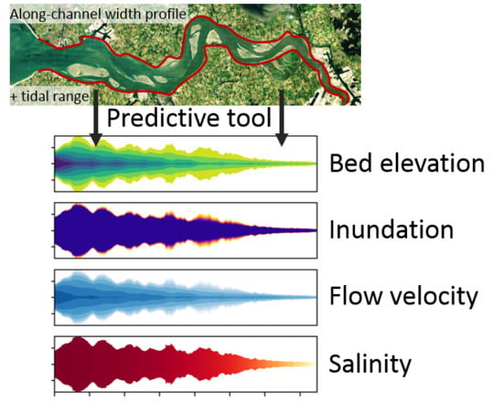
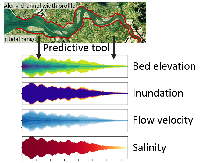
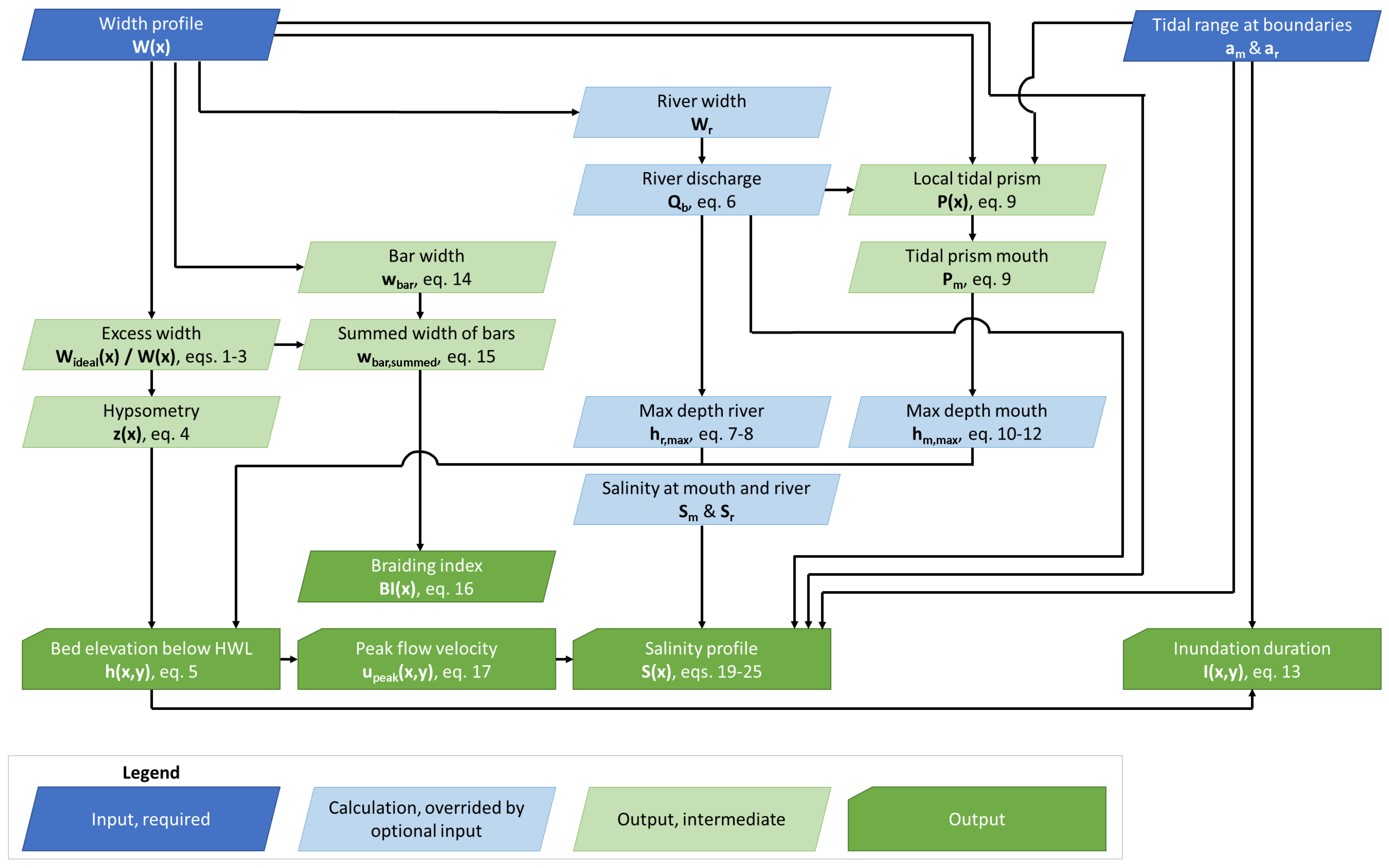
2.1. Tool Approach
2.2. Bed Elevation Prediction
2.2.1. Estuary Shape Predicts Cross-Sectional Hypsometry
2.2.2. Tidal Prism and River Discharge Predict Channel Geometry at the Mouth and Landward River
2.3. Inundation Duration Prediction
2.4. Bar Pattern Prediction: Bar Width and Braiding Index
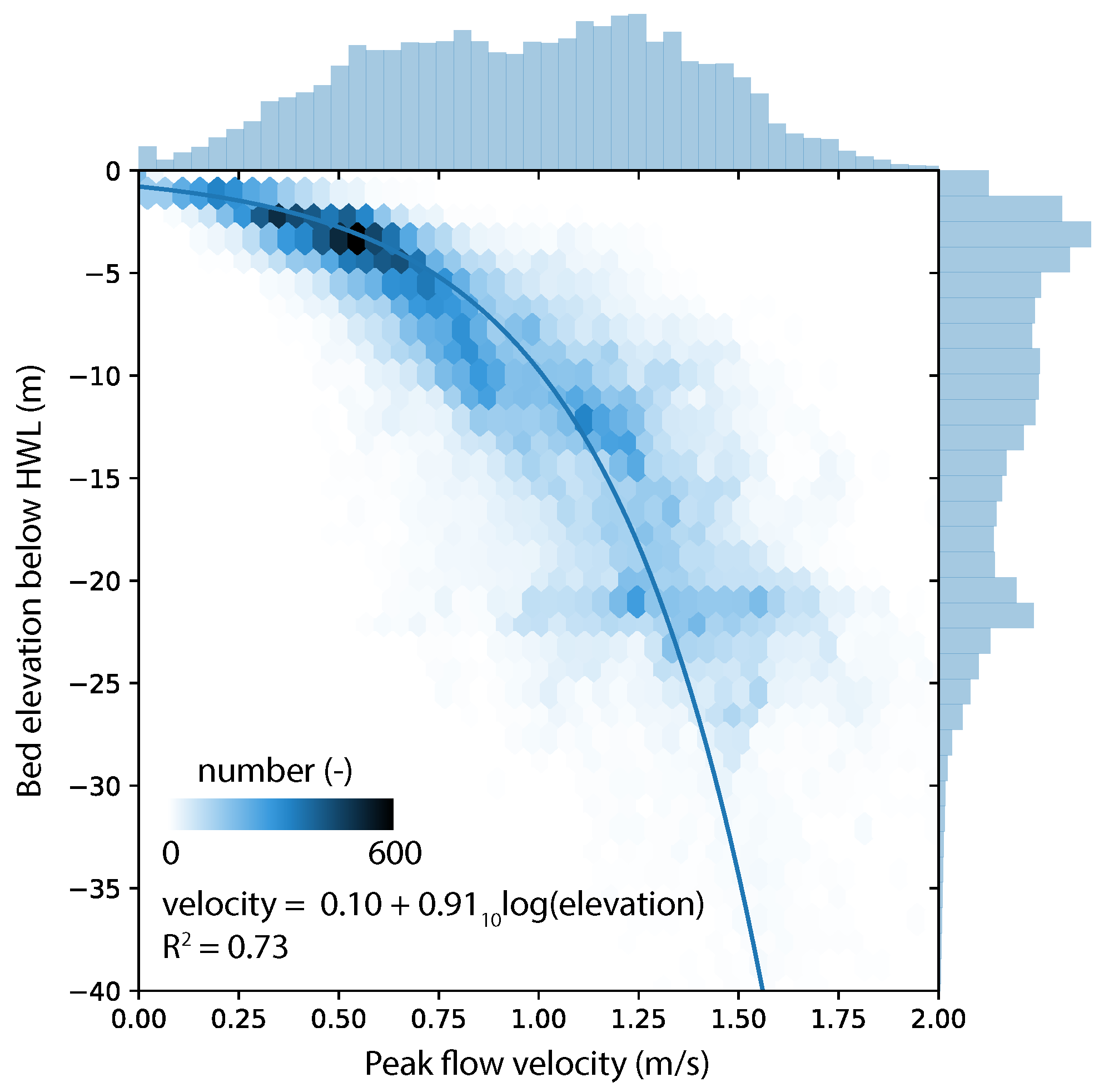
2.5. Flow Velocity Prediction
2.6. Salinity Prediction
2.7. Tool Validation
2.8. Tool Application to End-Member Cases
3. Results
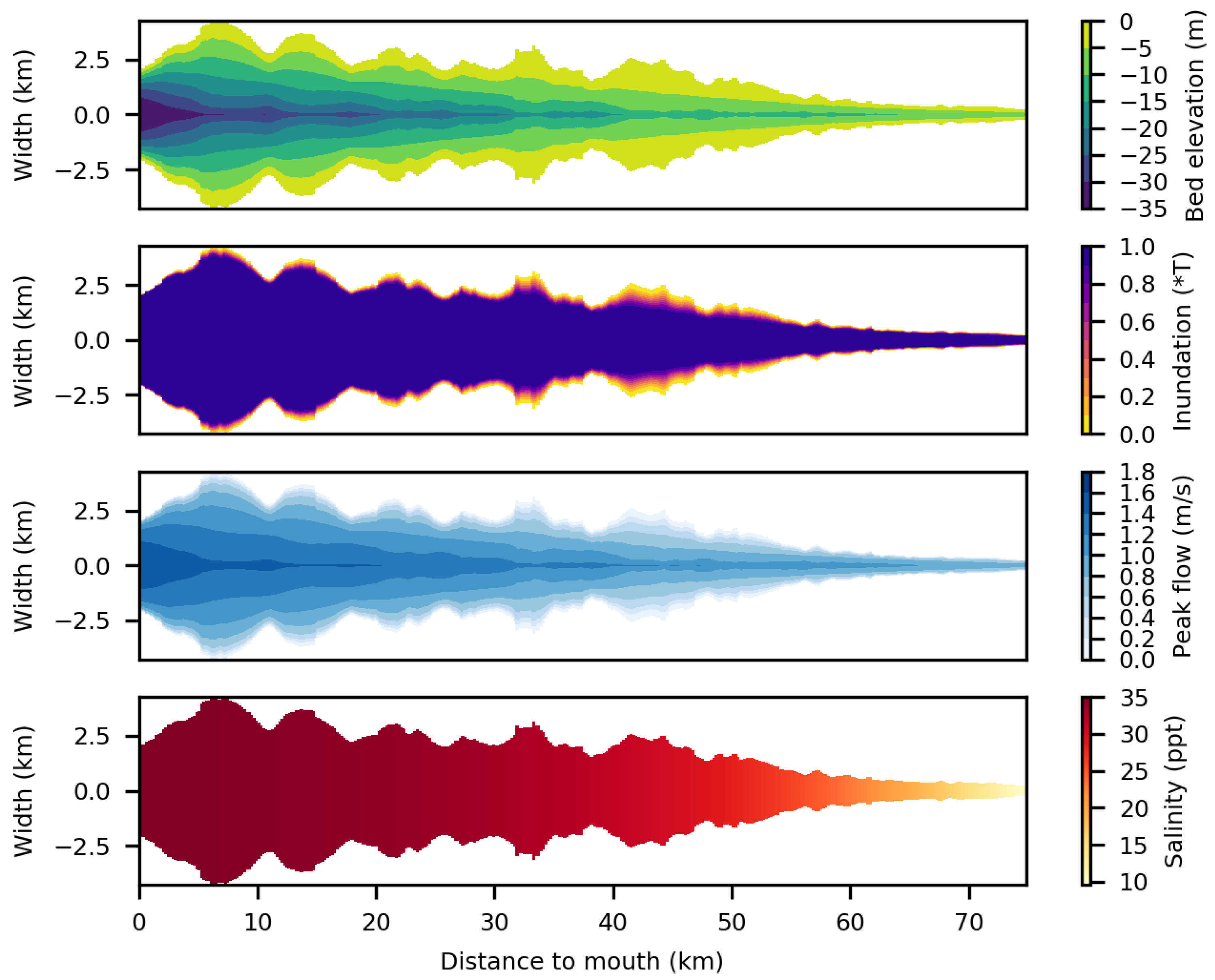
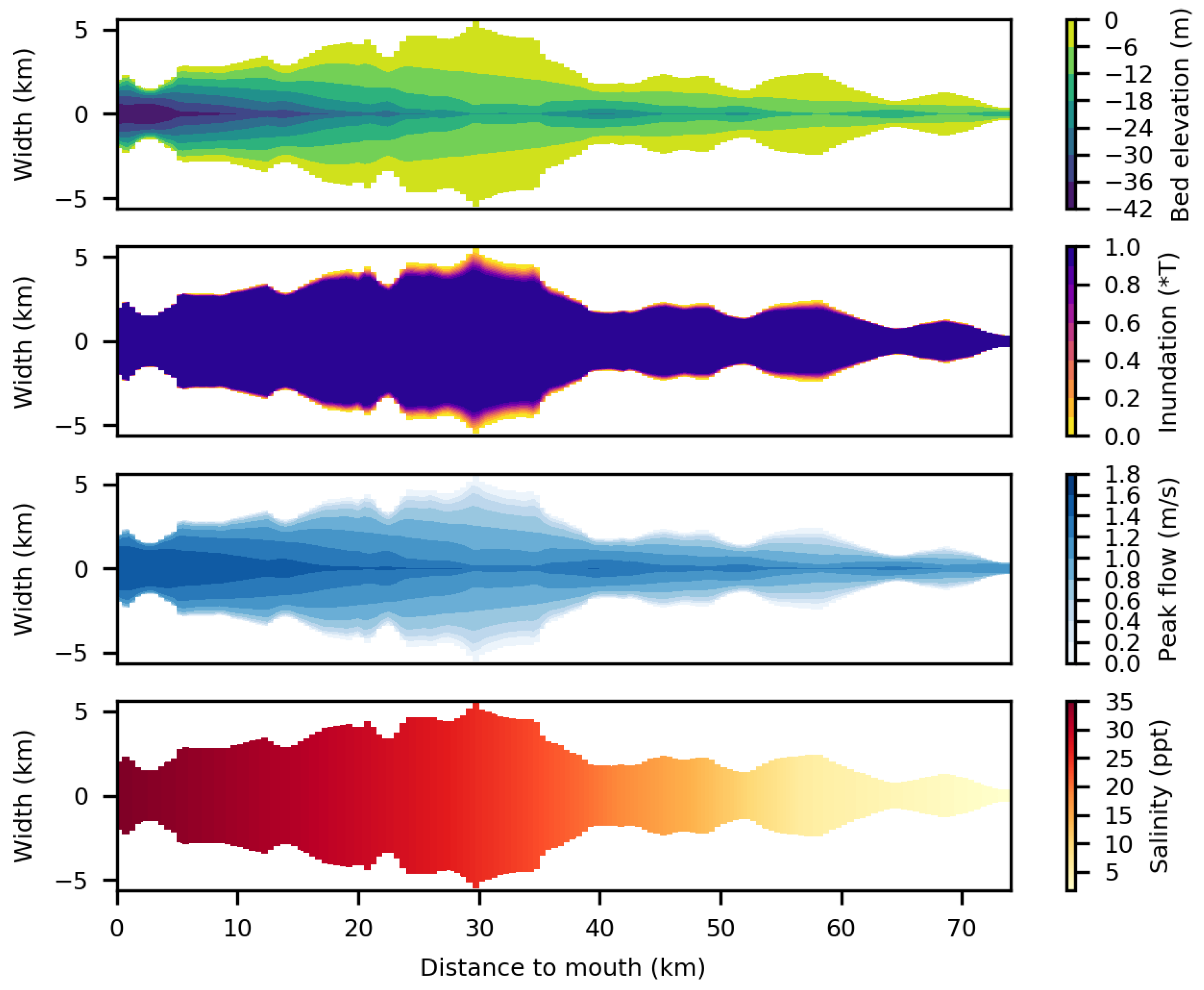
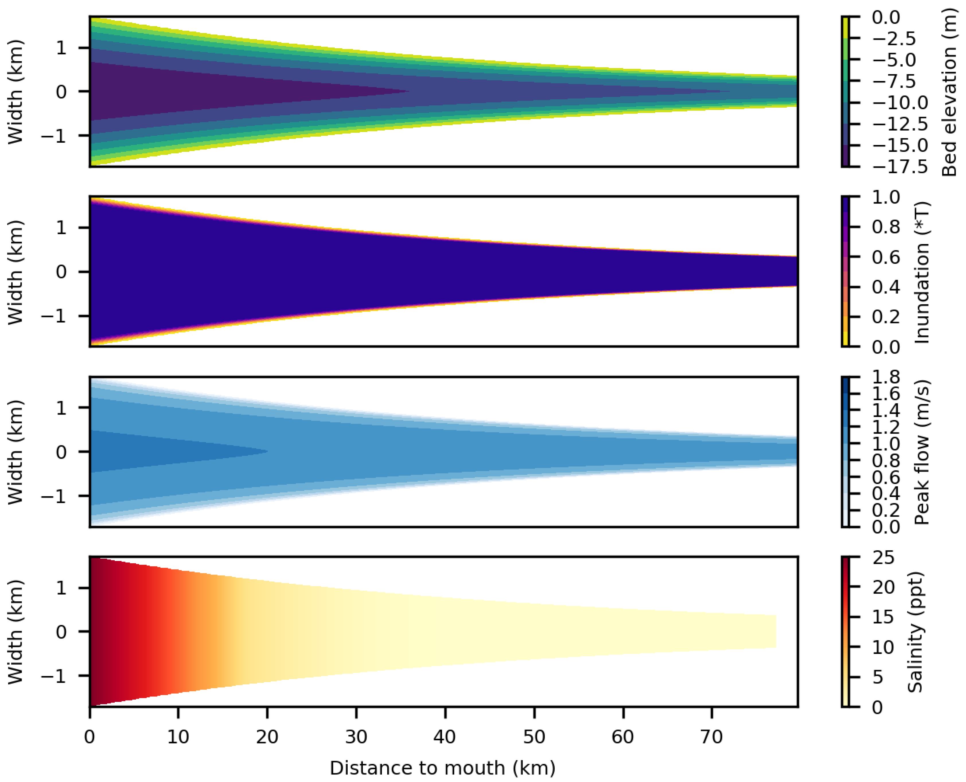
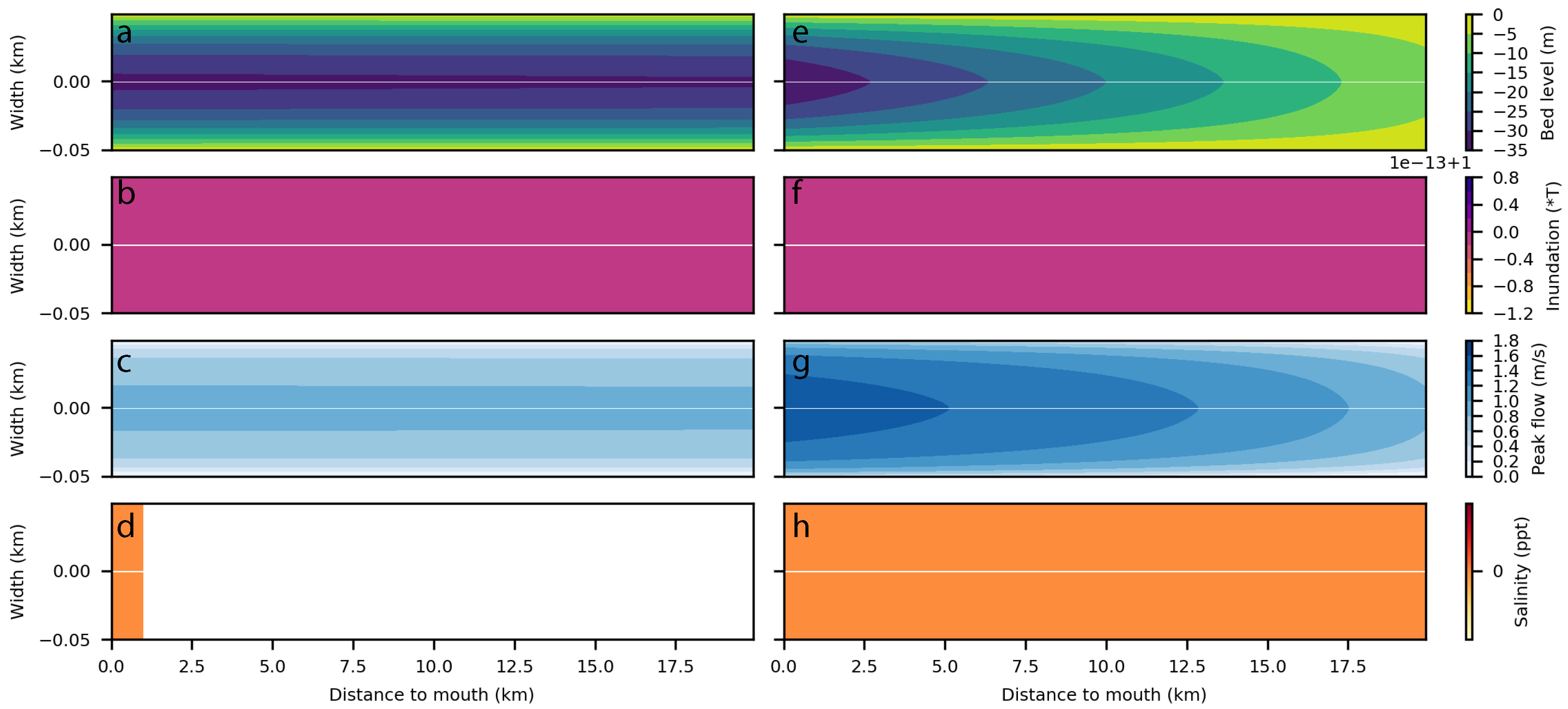
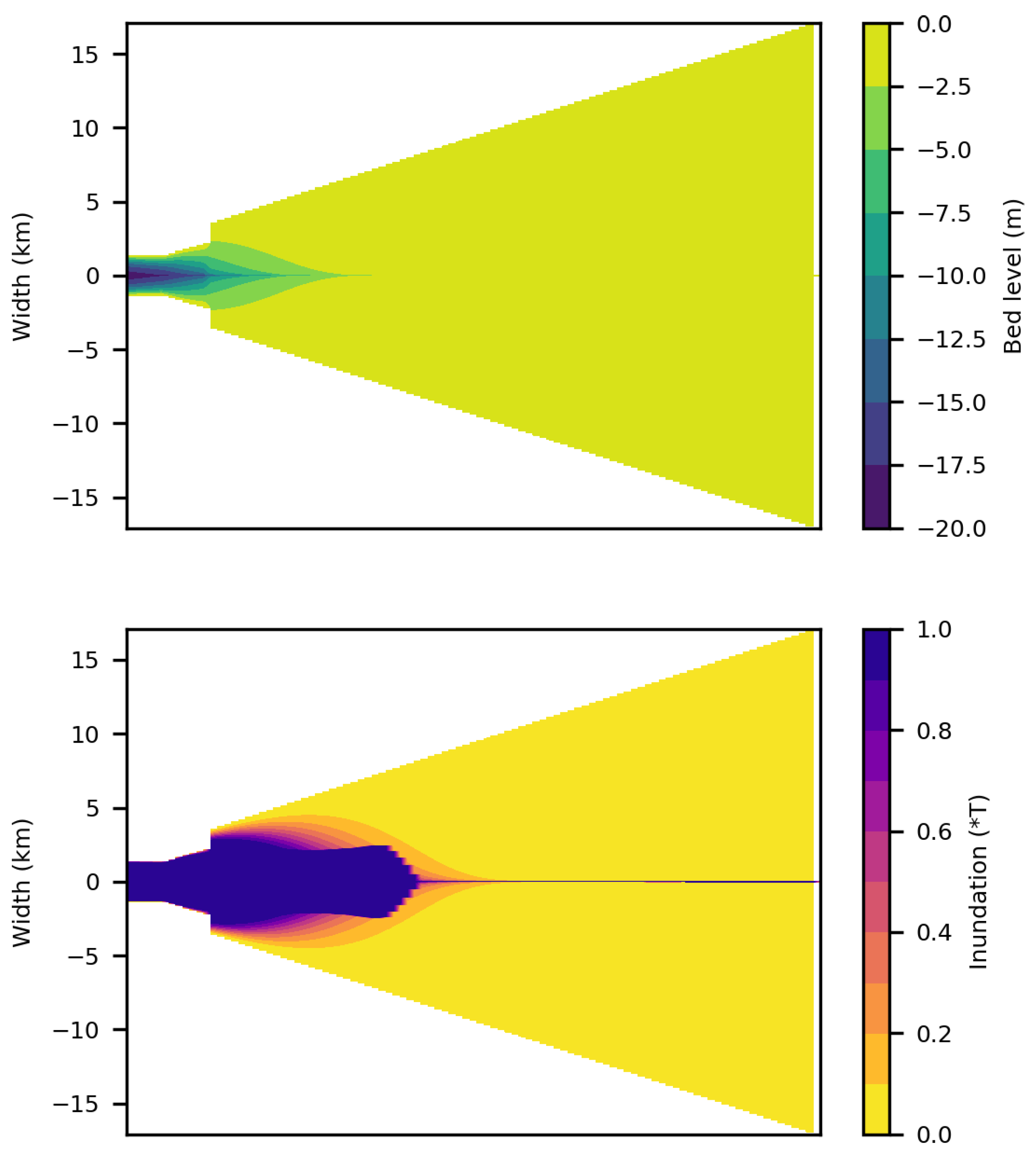
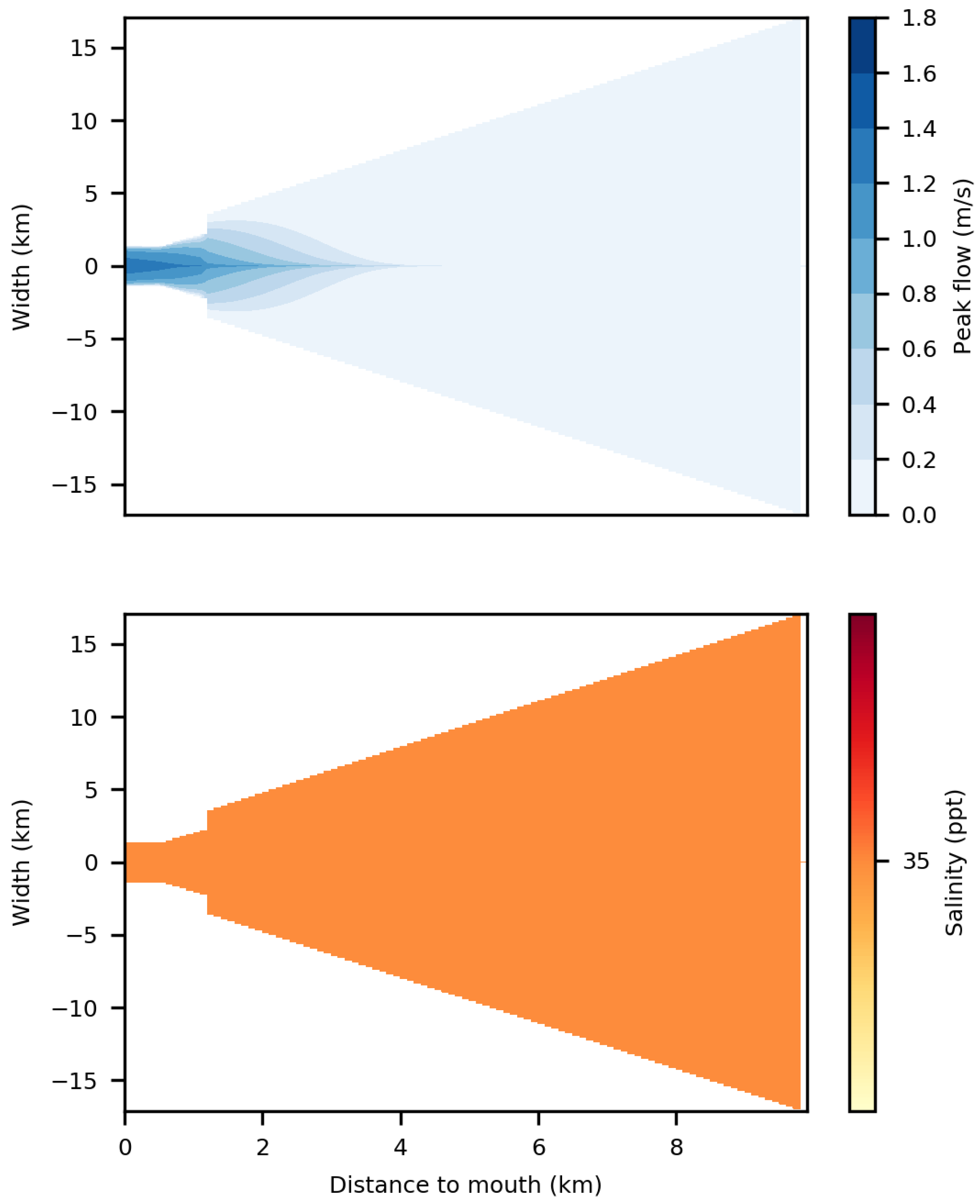
3.1. Tool Output
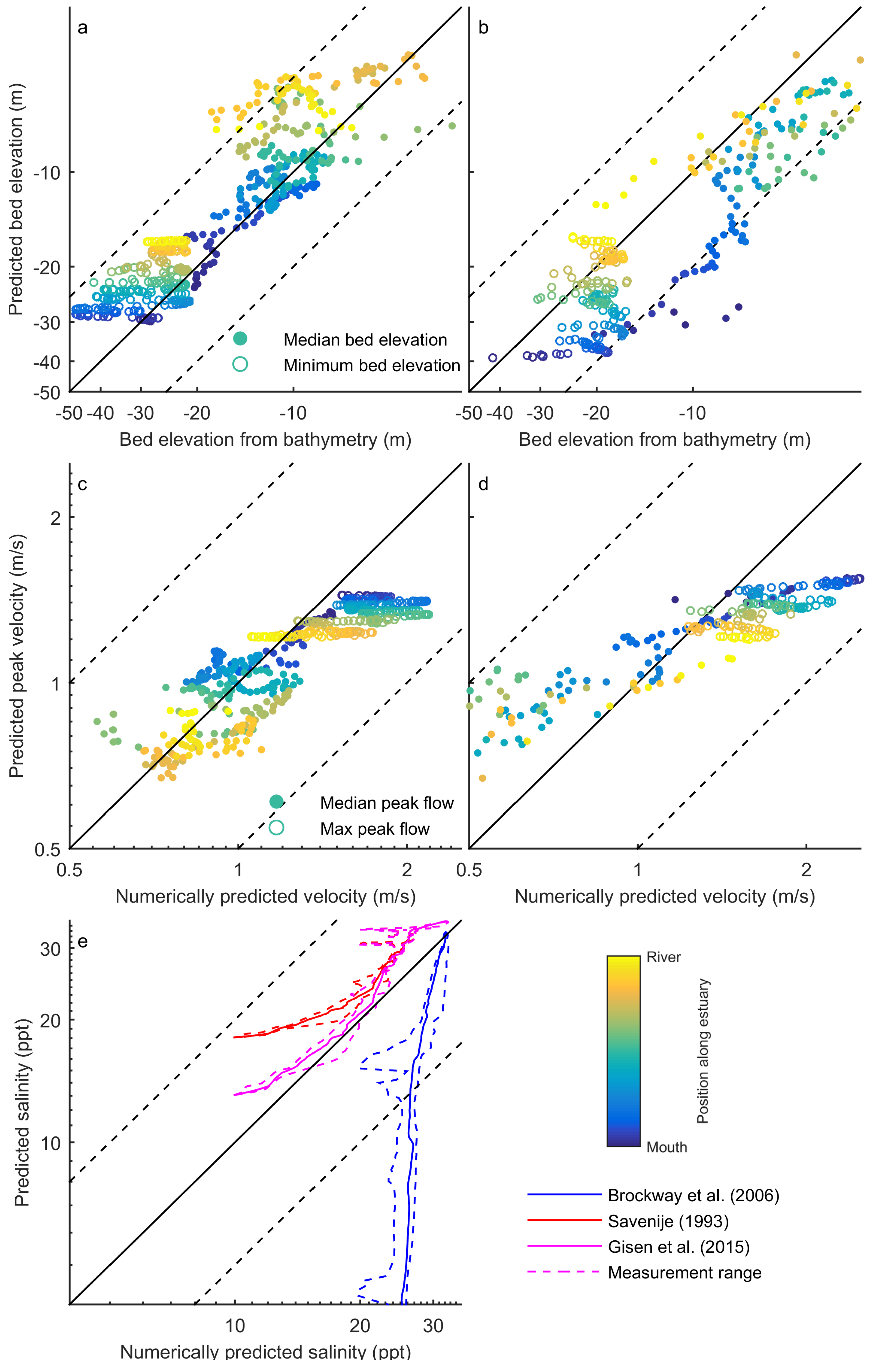
3.2. Tool Validation
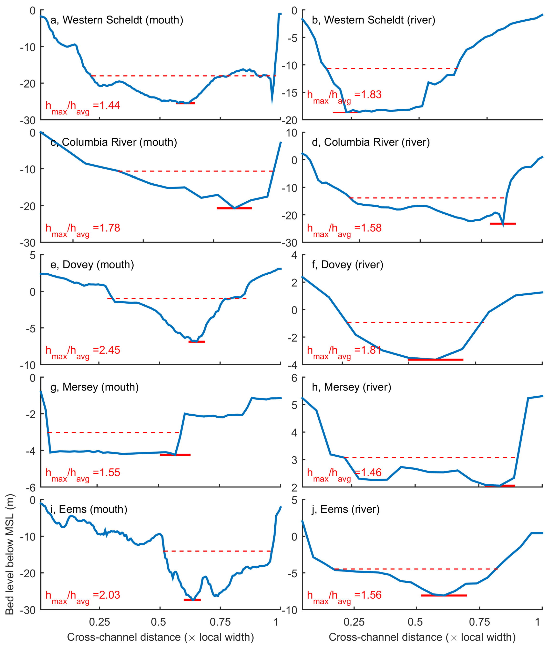
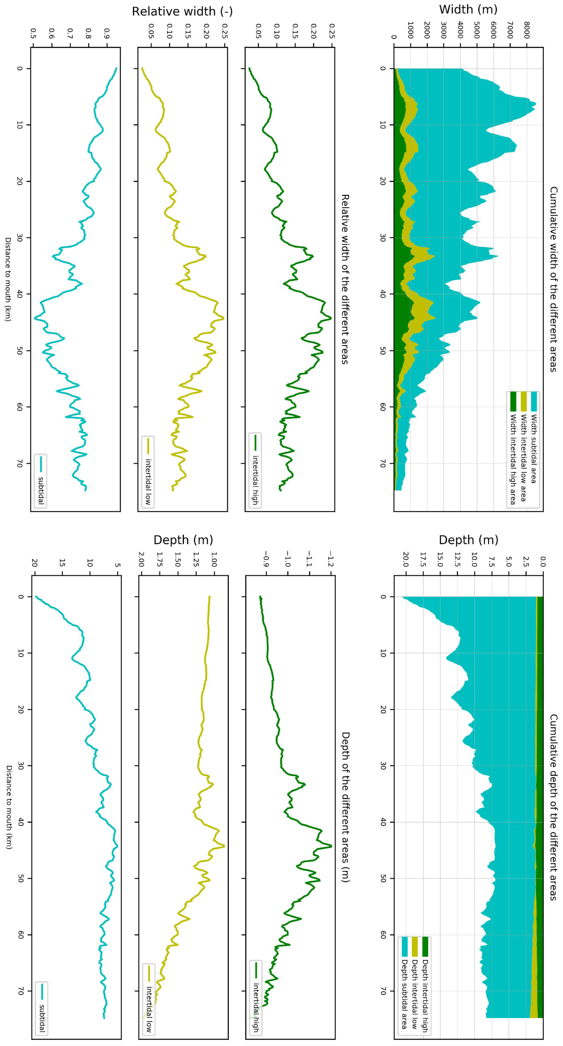
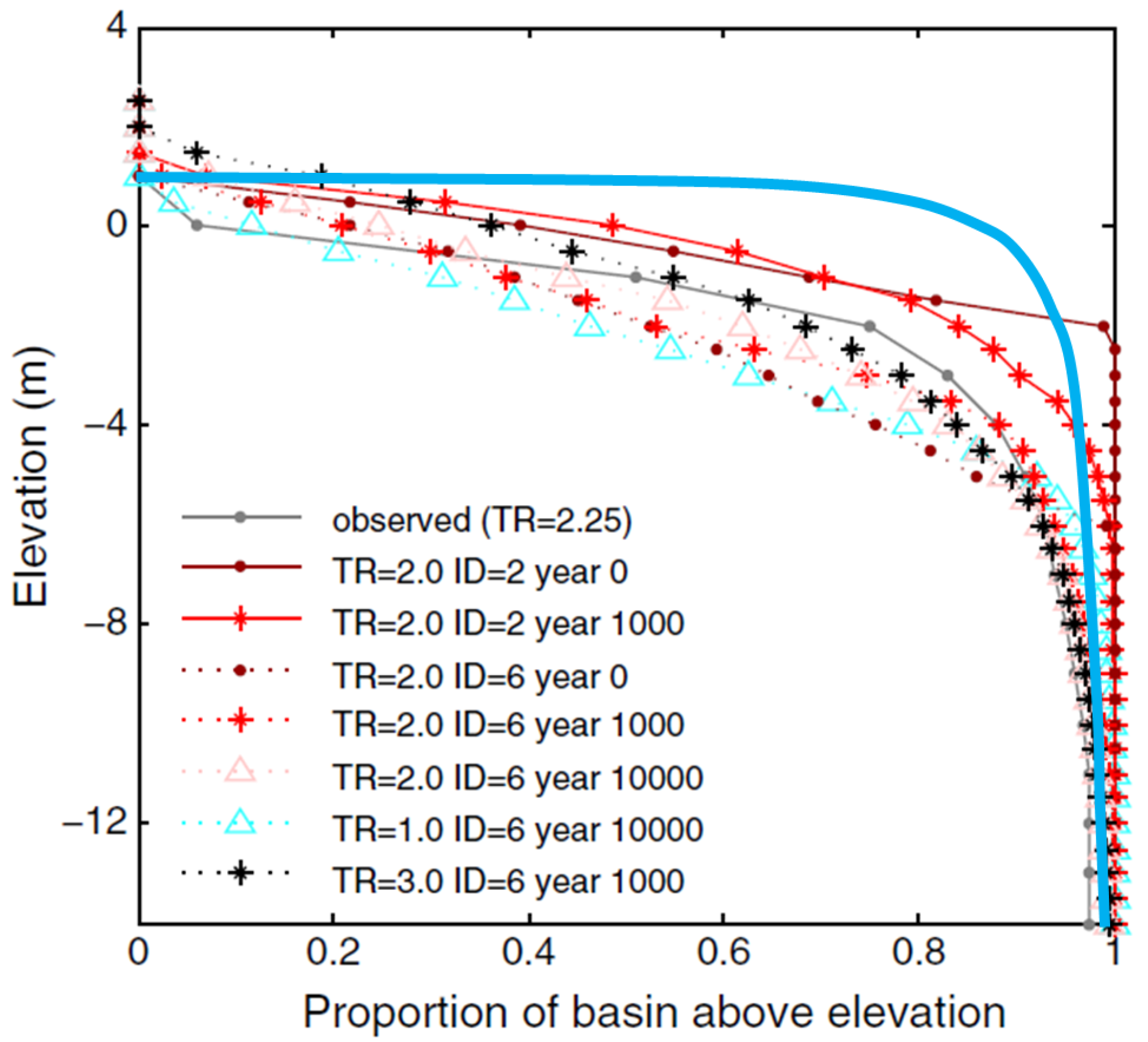
3.2.1. Bed Elevations
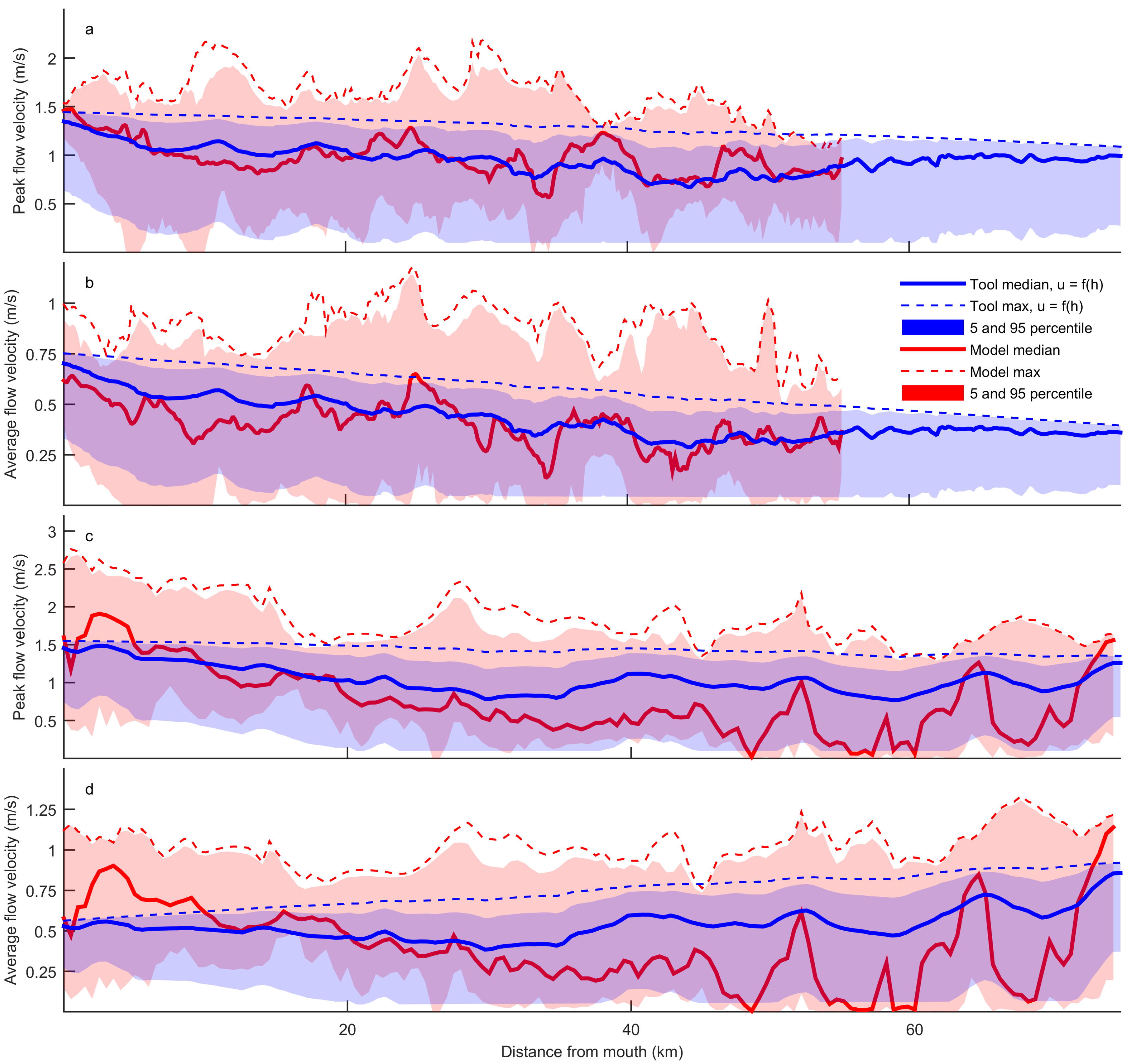
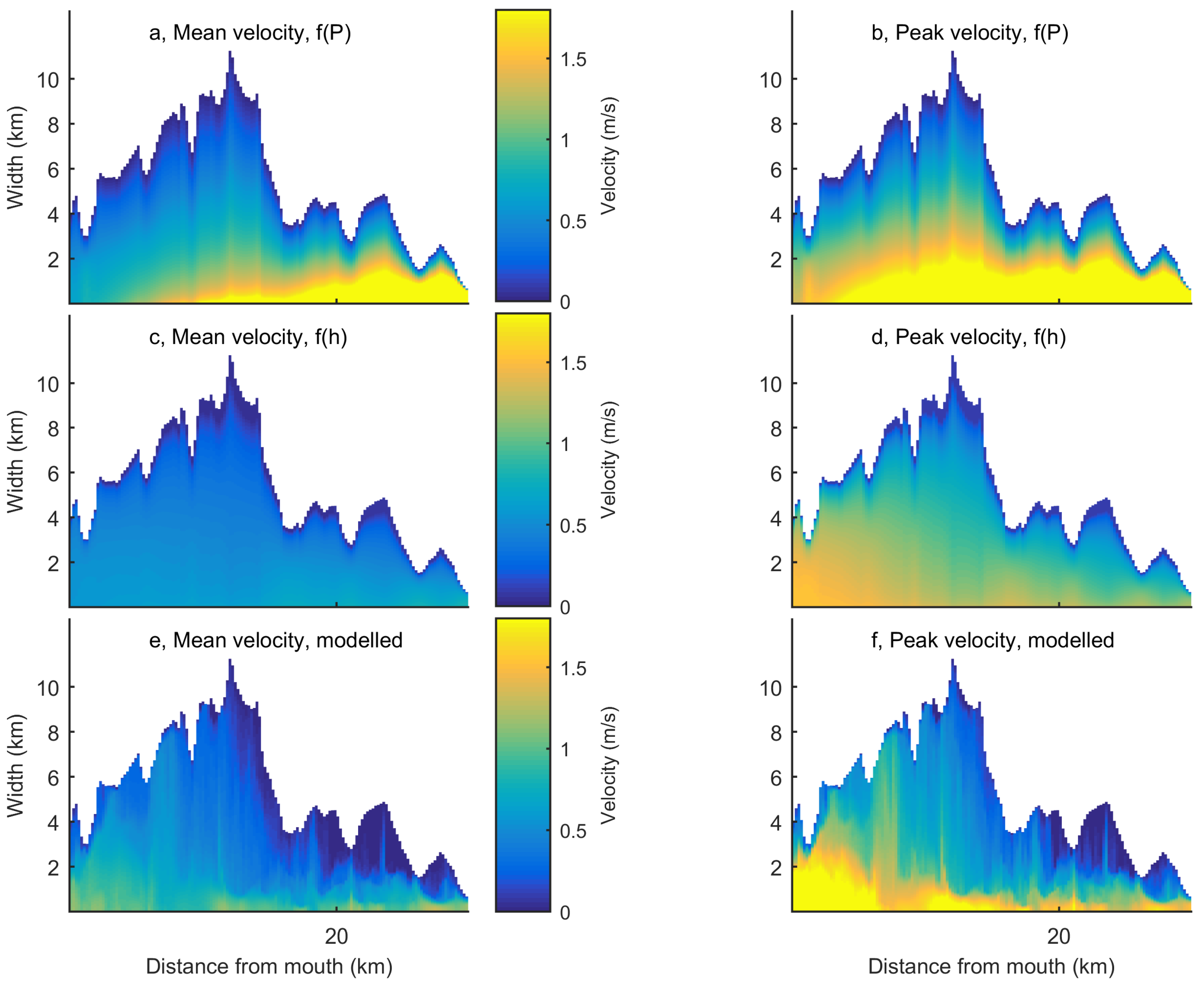
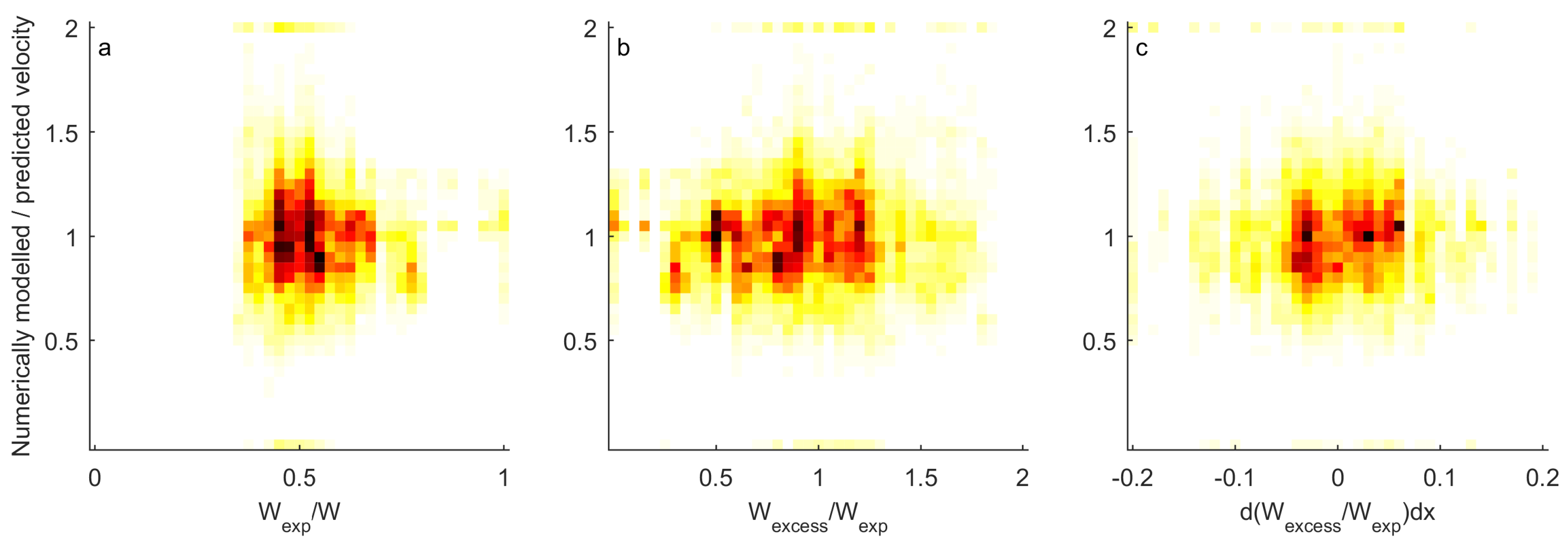
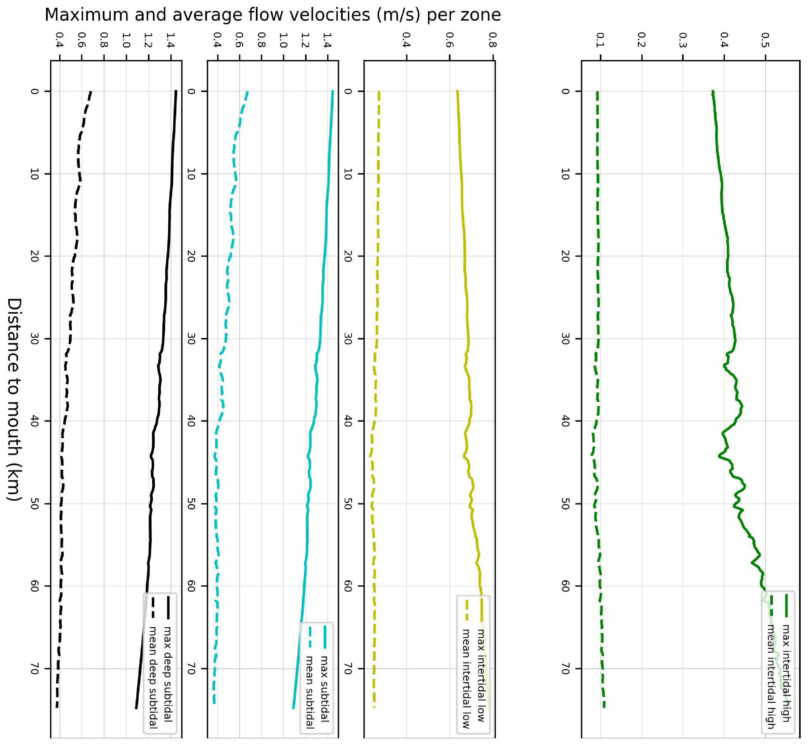
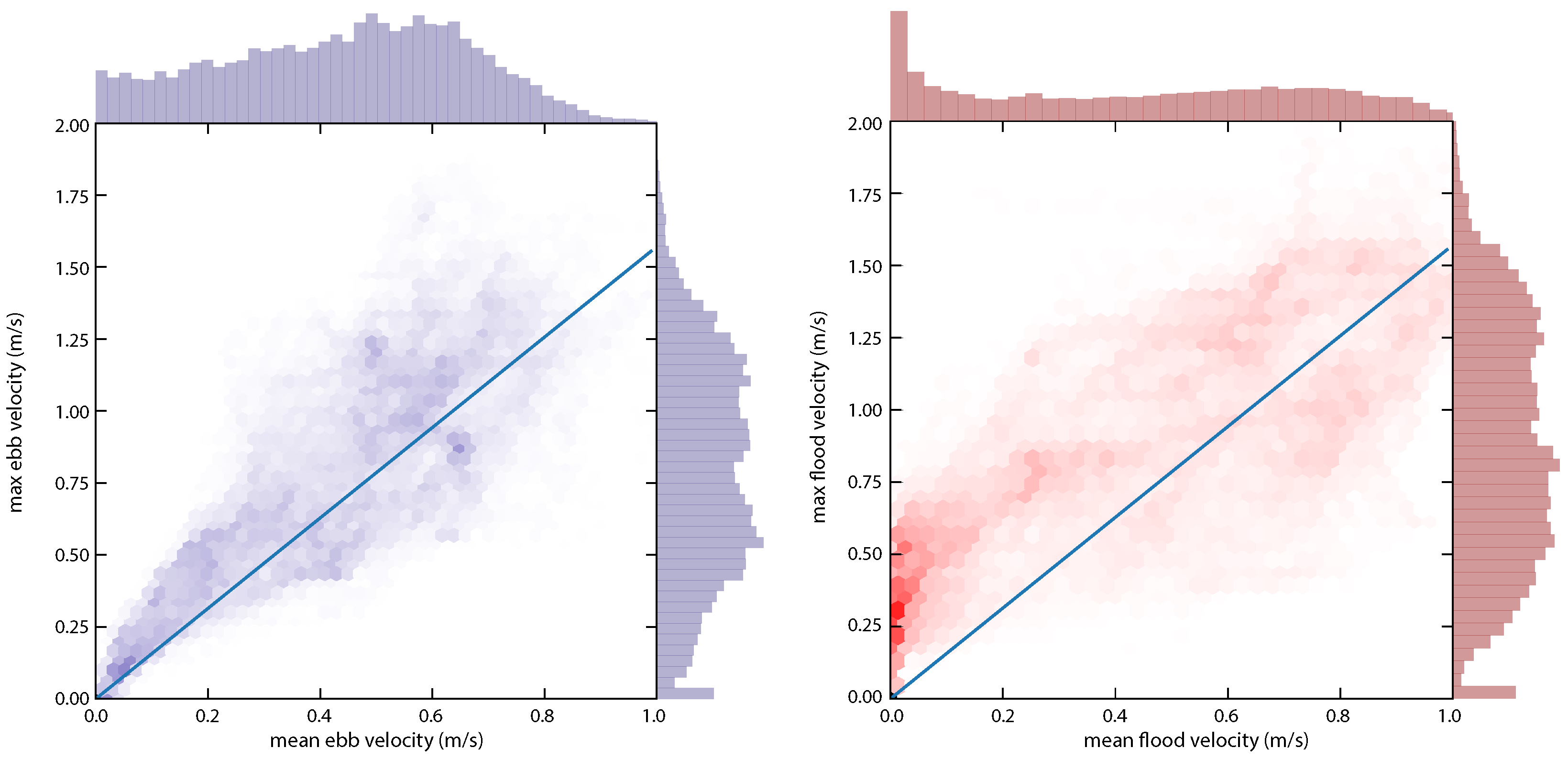
3.2.2. Flow Velocity
3.2.3. Salinity
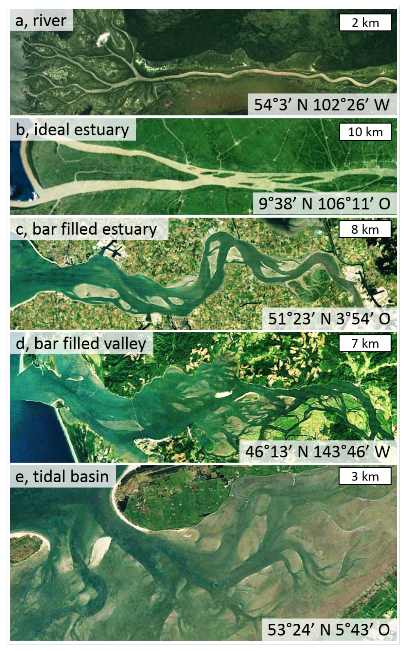
3.3. Applicability to End-Member Systems: A River, an Ideal Estuary, and a Tidal Basin
4. Discussion
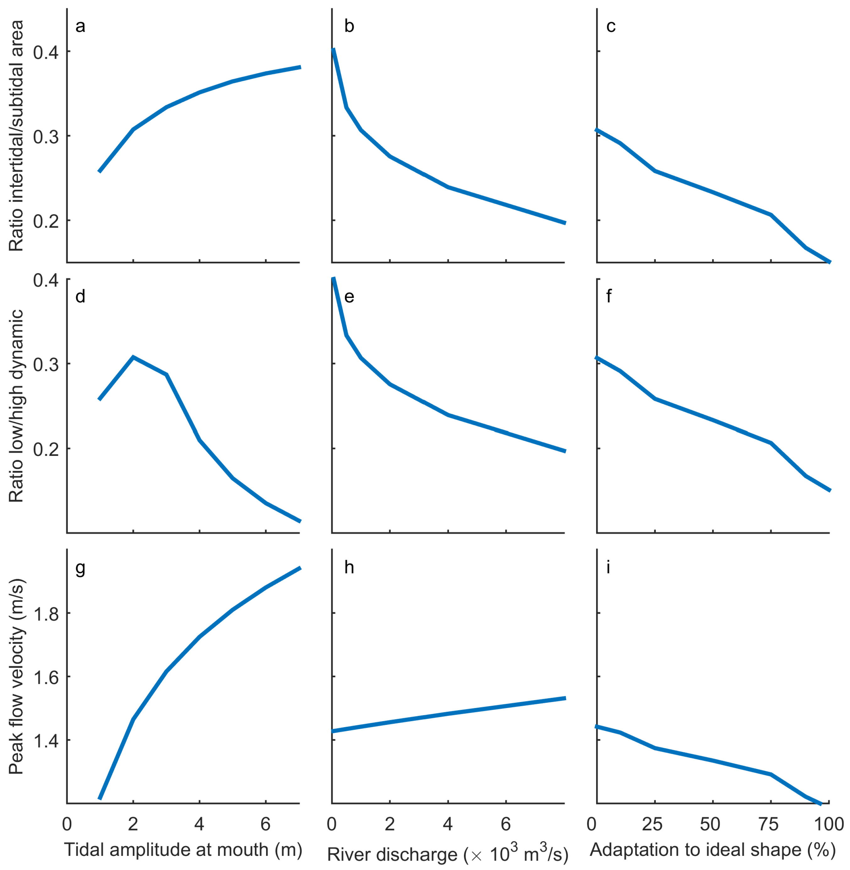
4.1. Sensitivity of Tool Output to Tidal Range, River Discharge, and along-Channel Width Profile
4.2. Applications
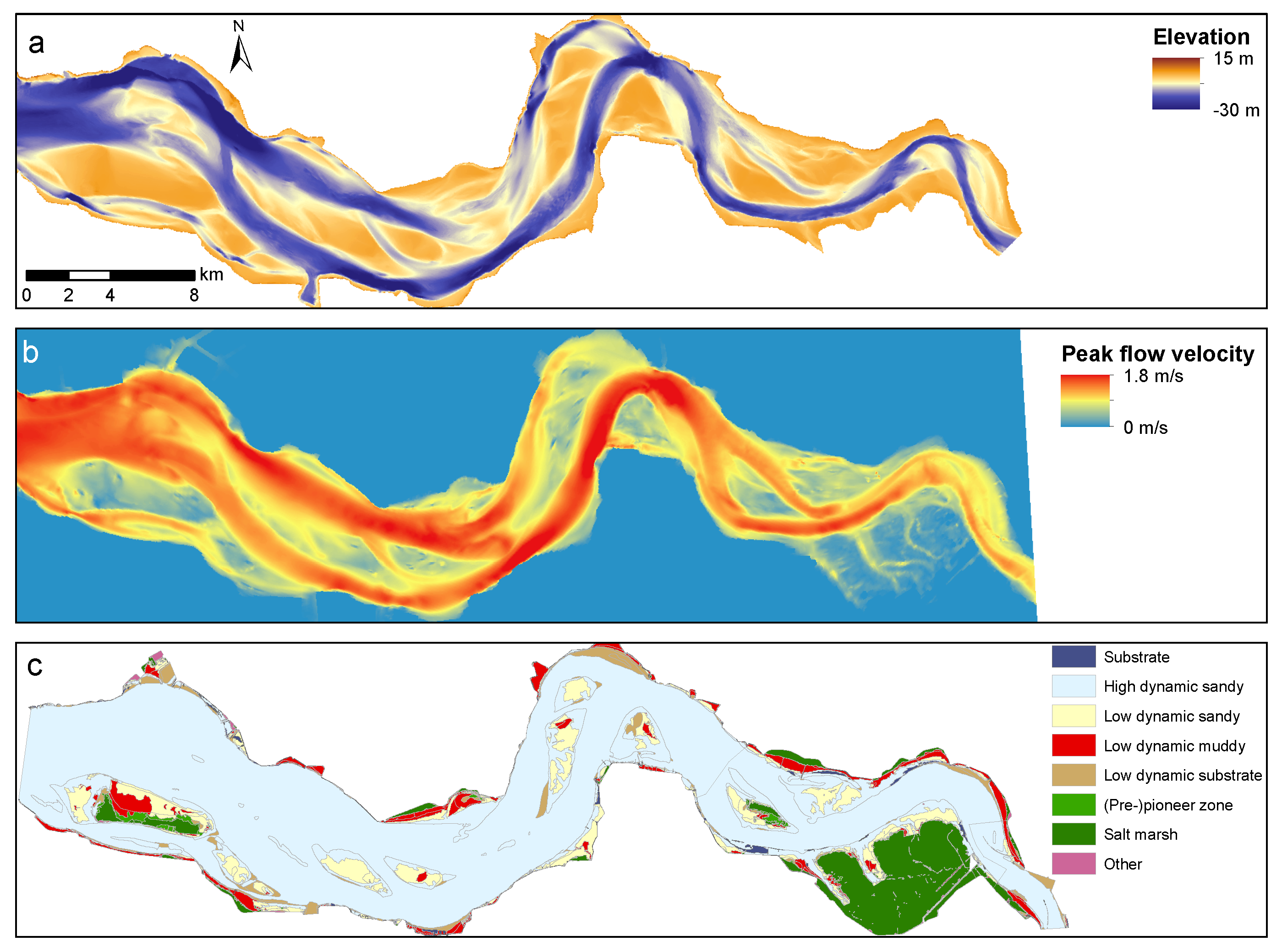
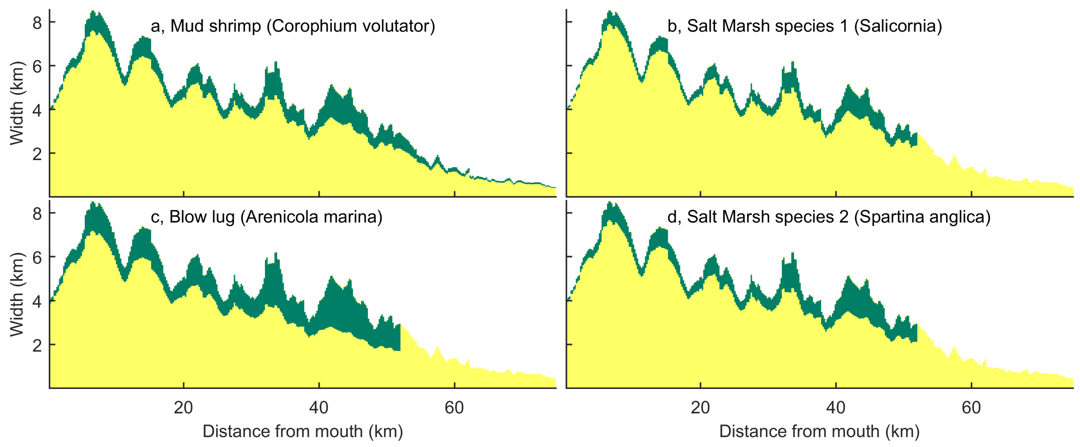
4.2.1. Illustration of Application for Ecological Assessment
4.2.2. Application for Management of Estuaries
4.2.3. Application in Palaeogeographic Reconstruction
5. Conclusions
Supplementary Materials
Author Contributions
Funding
Acknowledgments
Conflicts of Interest
Appendix A. Supplementary Figures and Table


| Symbol | Units | Variable |
|---|---|---|
| [m] | Cross-sectional area at the mouth | |
| [m] | Cross-sectional area at coordinate x | |
| [m] | Tidal range at the mouth | |
| [m] | Tidal range at the mouth | |
| [-] | Braiding Index at coordinate x | |
| [ms] | Chezy roughness at the estuary mouth | |
| [ms] | Dispersion coefficient at the mouth of the estuary | |
| [ms] | Dispersion coefficient at coordinate x | |
| [-] | Density difference between salt and fresh water | |
| E | [m] | Tidal excursion length |
| g | [ms] | Gravitational acceleration |
| [m] | Maximum channel depth at the landward boundary | |
| [m] | Average channel depth at the landward boundary | |
| [m] | Maximum channel depth at the estuary mouth | |
| [m] | Average channel depth at the estuary mouth | |
| [-] | Dimensionless bed elevation at coordinate (x,y) | |
| [m] | Dimensional bed elevation at coordinate (x,y) | |
| [× t] | Inundation duration | |
| K | [ms] | Empirical equation for the longitudinal mixing coefficient |
| [-] | Longitudinal Van der Burgh mixing coefficient in Savenije [21] | |
| [-] | Longitudinal Van der Burgh mixing coefficient in Gisen et al. [23] | |
| [m] | Width convergence length | |
| [m] | Cross-sectional area convergence length | |
| [-] | Estuarine Richardson number | |
| [m] | Local tidal prism at coordinate x | |
| [m] | Local tidal prism at the estuary mouth | |
| [ms] | Bankfull river discharge | |
| [ms] | Average river discharge | |
| r | [-] | Coefficient in the Strahler [33] equation |
| [-] | Storage ratio (intertidal area/subtidal area) | |
| [kgm] | Water density | |
| [ppt] | Salinity at the estuary mouth | |
| [ppt] | Salinity at the landward boundary | |
| [ppt] | Salinity at coordinate x [22] | |
| [ppt] | Salinity at coordinate x [23] | |
| [ppt] | Salinity at coordinate x [21] | |
| s | [s] | Distance between the mouth and landward boundary |
| [-] | Shape factor of the channel at the estuary mouth | |
| [-] | Shape factor of the channel at the landward boundary | |
| t | [s] | Duration of half a tidal cycle |
| [ms] | Tidal average flow velocity at coordinate (x,y) | |
| [ms] | Peak tidal flow velocity at coordinate (x,y) | |
| [ms] | Peak tidal flow velocity at the estuary mouth | |
| [m] | Excess width at coordinate x | |
| [m] | Ideal width at coordinate x | |
| [m] | Width at the estuary mouth | |
| [m] | Width at the landward boundary | |
| [m] | Local width at coordinate x | |
| [m] | Predicted bar width at coordinate x | |
| [m] | Summed width of bars at coordinate x | |
| x | [m] | Streamwise coordinate measured from the mouth along the centreline |
| y | [m] | Coordinate perpendicular to the centreline |
| z | [-] | Coefficient in the Strahler [33] equation |
| [-] | Value of z-coefficient at coordinate x |
References
- De Vriend, H.J.; Wang, Z.B.; Ysebaert, T.; Herman, P.M.; Ding, P. Eco-morphological problems in the Yangtze Estuary and the Western Scheldt. Wetlands 2011, 31, 1033–1042. [Google Scholar] [CrossRef]
- Bouma, H.; de Jong, D.; Twisk, F.; Wolfstein, K. A Dutch Ecotope System for Coastal Waters (ZES. 1). To Map the Potential Occurence of Ecological Communities in Dutch Coastal And Transitional Waters; Technical Report, Rijkswaterstaat, Report RIKZ/2005.024; Rijksinstituut voor Kust en Zee/RIKZ: Middelburg, The Netherlands, 2005. [Google Scholar]
- De Jong, D. Ecotopes in the Dutch Marine Tidal Waters: A Proposal for a Classification of Ecotopes and a Method to Map Them; Technical Report, Rijkswaterstaat, Report RIKZ/99.017; Rijksinstituut voor Kust en Zee/RIKZ: Middelburg, The Netherlands, 1999. [Google Scholar]
- Gurnell, A.M.; Bertoldi, W.; Corenblit, D. Changing river channels: The roles of hydrological processes, plants and pioneer fluvial landforms in humid temperate, mixed load, gravel bed rivers. Earth-Sci. Rev. 2012, 111, 129–141. [Google Scholar] [CrossRef]
- Cozzoli, F.; Smolders, S.; Eelkema, M.; Ysebaert, T.; Escaravage, V.; Temmerman, S.; Meire, P.; Herman, P.M.; Bouma, T.J. A modeling approach to assess coastal management effects on benthic habitat quality: A case study on coastal defense and navigability. Estuar. Coast. Shelf Sci. 2017, 184, 67–82. [Google Scholar] [CrossRef] [Green Version]
- Van der Wegen, M.; Roelvink, J. Reproduction of estuarine bathymetry by means of a process-based model: Western Scheldt case study, the Netherlands. Geomorphology 2012, 179, 152–167. [Google Scholar] [CrossRef]
- Elias, E.P.; Gelfenbaum, G.; Van der Westhuysen, A.J. Validation of a coupled wave-flow model in a high-energy setting: The mouth of the Columbia River. J. Geophys. Res. Oceans 2012, 117, C09011. [Google Scholar] [CrossRef]
- Braat, L.; van Kessel, T.; Leuven, J.R.F.W.; Kleinhans, M.G. Effects of mud supply on large-scale estuary morphology and development over centuries to millennia. Earth Surf. Dyn. 2017, 5, 617–652. [Google Scholar] [CrossRef] [Green Version]
- Townend, I. The estimation of estuary dimensions using a simplified form model and the exogenous controls. Earth Surf. Process. Landf. 2012, 37, 1573–1583. [Google Scholar] [CrossRef]
- Seminara, G.; Tubino, M. Sand bars in tidal channels. Part 1. Free bars. J. Fluid Mech. 2001, 440, 49–74. [Google Scholar] [CrossRef]
- Schramkowski, G.; Schuttelaars, H.; De Swart, H. The effect of geometry and bottom friction on local bed forms in a tidal embayment. Cont. Shelf Res. 2002, 22, 1821–1833. [Google Scholar] [CrossRef] [Green Version]
- Leuven, J.R.F.W.; Kleinhans, M.G.; Weisscher, S.A.H.; van der Vegt, M. Tidal sand bar dimensions and shapes in estuaries. Earth-Sci. Rev. 2016, 161, 204–233. [Google Scholar] [CrossRef]
- O’Brien, M.P. Equilibrium flow areas of inlets on sandy coasts. In Journal of the Waterways and Harbors Division: Proceedings of the American Society of Civil Engineers (ASCE); American Society of Civil Engineers: New York, NY, USA, 1969; pp. 43–52. [Google Scholar] [CrossRef]
- Wang, Z.; Jeuken, C.; De Vriend, H. Tidal Asymmetry and Residual Sediment Transport in Estuaries; Delft Hydraulics Report Z2749; Deltares (WL): Delft, The Netherlands, 1999. [Google Scholar]
- Lanzoni, S.; D’Alpaos, A. On funneling of tidal channels. J. Geophys. Res. Earth Surf. 2015, 120, 433–452. [Google Scholar] [CrossRef] [Green Version]
- Zhou, Z.; Coco, G.; Townend, I.; Gong, Z.; Wang, Z.; Zhang, C. On the stability relationships between tidal asymmetry and morphologies of tidal basins and estuaries. Earth Surf. Process. Landf. 2018, 43, 1943–1959. [Google Scholar] [CrossRef]
- Langbein, W. The hydraulic geometry of a shallow estuary. Hydrol. Sci. J. 1963, 8, 84–94. [Google Scholar] [CrossRef]
- Savenije, H.H. Salinity and Tides in Alluvial Estuaries; Elsevier: Amsterdam, The Netherlands, 2006. [Google Scholar]
- Leuven, J.R.F.W.; Haas, T.; Braat, L.; Kleinhans, M.G. Topographic forcing of tidal sand bar patterns for irregular estuary planforms. Earth Surf. Process. Landf. 2018, 43, 172–186. [Google Scholar] [CrossRef]
- Leuven, J.R.F.W.; Selaković, S.; Kleinhans, M.G. Morphology of bar-built estuaries: empirical relation between planform shape and depth distribution. Earth Surf. Dyn. 2018, 6, 763–778. [Google Scholar] [CrossRef]
- Savenije, H.H. Predictive model for salt intrusion in estuaries. J. Hydrol. 1993, 148, 203–218. [Google Scholar] [CrossRef]
- Brockway, R.; Bowers, D.; Hoguane, A.; Dove, V.; Vassele, V. A note on salt intrusion in funnel-shaped estuaries: Application to the Incomati estuary, Mozambique. Estuar. Coast. Shelf Sci. 2006, 66, 1–5. [Google Scholar] [CrossRef]
- Gisen, J.; Savenije, H.; Nijzink, R. Revised predictive equations for salt intrusion modelling in estuaries. Hydrol. Earth Syst. Sci. 2015, 19, 2791–2803. [Google Scholar] [CrossRef]
- Haasnoot, M.; van de Wolfshaar, K. Combining a conceptual framework and a spatial analysis tool, HABITAT, to support the implementation of river basin management plans. Int. J. River Basin Manag. 2009, 7, 295–311. [Google Scholar] [CrossRef]
- Van Oorschot, M.; Kleinhans, M.; Buijse, T.; Geerling, G.; Middelkoop, H. Combined effects of climate change and dam construction on riverine ecosystems. Ecol. Eng. 2018, 120, 329–344. [Google Scholar] [CrossRef]
- Dalrymple, R.W.; Zaitlin, B.A.; Boyd, R. Estuarine facies models: Conceptual basis and stratigraphic implications: Perspective. J. Sediment. Res. 1992, 62. [Google Scholar] [CrossRef]
- De Haas, T.; Pierik, H.; van der Spek, A.; Cohen, K.; van Maanen, B.; Kleinhans, M. Holocene evolution of tidal systems in The Netherlands: Effects of rivers, coastal boundary conditions, eco-engineering species, inherited relief and human interference. Earth-Sci. Rev. 2017, 177, 139–163. [Google Scholar] [CrossRef]
- Stevens, A.; Gelfenbaum, G.; MacMahan, J.; Reniers, A.; Elias, E.; Sherwood, C.; Carlson, E. Oceanographic Measurements and Hydrodynamic Modeling of the Mouth of the Columbia River, Oregon and Washington, 2013; Technical Report; U.S. Geological Survey: Reston, VA, USA, 2017. [CrossRef]
- Marciano, R.; Wang, Z.B.; Hibma, A.; de Vriend, H.J.; Defina, A. Modeling of channel patterns in short tidal basins. J. Geophys. Res. Earth Surf. 2005, 110, F01001. [Google Scholar] [CrossRef]
- Wang, Z.B.; Hoekstra, P.; Burchard, H.; Ridderinkhof, H.; De Swart, H.E.; Stive, M.J.F. Morphodynamics of the Wadden Sea and its barrier island system. Ocean Coast. Manag. 2012, 68, 39–57. [Google Scholar] [CrossRef]
- van Maanen, B.; Coco, G.; Bryan, K.R. Modelling the effects of tidal range and initial bathymetry on the morphological evolution of tidal embayments. Geomorphology 2013, 191, 23–34. [Google Scholar] [CrossRef]
- Verbeek, H.; Van der Male, K.; Jansen, M. Het SCALWEST-model (in Dutch); Technical Report, Technical Report RIKZ/OS/2000.814; Rijksinstituut voor Kust en Zee/RIKZ: Middelburg, The Netherlands, 2000. [Google Scholar]
- Strahler, A.N. Hypsometric (area-altitude) analysis of erosional topography. Geol. Soc. Am. Bull. 1952, 63, 1117–1142. [Google Scholar] [CrossRef]
- Boon, J.D.; Byrne, R.J. On basin hyposmetry and the morphodynamic response of coastal inlet systems. Mar. Geol. 1981, 40, 27–48. [Google Scholar] [CrossRef]
- Townend, I.H. Hypsometry of estuaries, creeks and breached sea wall sites. Proc. Inst. Civ. Eng.-Marit. Eng. 2008, 161, 23–32. [Google Scholar] [CrossRef]
- Leopold, L.B.; Maddock, T., Jr. The Hydraulic Geometry of Stream Channels and Some Physiographic Implications; Technical Report, U.S. Geological Survey, Professional Paper 252; U.S. Geological Survey: Reston, VA, USA, 1953.
- Hey, R.D.; Thorne, C.R. Stable channels with mobile gravel beds. J. Hydraul. Eng. 1986, 112, 671–689. [Google Scholar] [CrossRef]
- Eysink, W. Morphologic response of tidal basins to changes. Coast. Eng. Proc. 1990, 1, 1948–1961. [Google Scholar] [CrossRef]
- Friedrichs, C.T. Stability shear stress and equilibrium cross-sectional geometry of sheltered tidal channels. J. Coast. Res. 1995, 11, 1062–1074. [Google Scholar]
- Pavelsky, T.M.; Smith, L.C. RivWidth: A software tool for the calculation of river widths from remotely sensed imagery. IEEE Geosci. Remote Sens. Lett. 2008, 5, 70–73. [Google Scholar] [CrossRef]
- Donchyts, G.; Schellekens, J.; Winsemius, H.; Eisemann, E.; van de Giesen, N. A 30 m resolution surface water mask including estimation of positional and thematic differences using landsat 8, srtm and openstreetmap: A case study in the Murray-Darling Basin, Australia. Remote Sens. 2016, 8, 386. [Google Scholar] [CrossRef]
- Savenije, H.H. Prediction in ungauged estuaries: An integrated theory. Water Resour. Res. 2015, 51, 2464–2476. [Google Scholar] [CrossRef] [Green Version]
- Davies, G.; Woodroffe, C.D. Tidal estuary width convergence: Theory and form in North Australian estuaries. Earth Surf. Process. Landf. 2010, 35, 737–749. [Google Scholar] [CrossRef]
- Pillsbury, G. Tidal Hydraulics, rev. ed.; US Army Corps of Engineers: Washington, DC, USA, 1956.
- Dronkers, J. Convergence of estuarine channels. Cont. Shelf Res. 2017, 144, 120–133. [Google Scholar] [CrossRef]
- Wang, Z.; Jeuken, M.; Gerritsen, H.; De Vriend, H.; Kornman, B. Morphology and asymmetry of the vertical tide in the Westerschelde estuary. Cont. Shelf Res. 2002, 22, 2599–2609. [Google Scholar] [CrossRef]
- Toffolon, M.; Crosato, A. Developing macroscale indicators for estuarine morphology: The case of the Scheldt Estuary. J. Coast. Res. 2007, 23, 195–212. [Google Scholar] [CrossRef]
- Jarrett, J.T. Tidal Prism-Inlet Area Relationships; Technical Report, DTIC Document WES-GITI-3; DTIC: Fort Belvoir, VA, USA, 1976.
- Shigemura, T. Tidal prism–throat area relationships of the bays of Japan. Shore Beach 1980, 48, 30–35. [Google Scholar]
- Gisen, J.I.A.; Savenije, H.H. Estimating bankfull discharge and depth in ungauged estuaries. Water Resour. Res. 2015, 51, 2298–2316. [Google Scholar] [CrossRef] [Green Version]
- Jay, D.A.; Smith, J.D. Circulation, density distribution and neap-spring transitions in the Columbia River Estuary. Prog. Oceanogr. 1990, 25, 81–112. [Google Scholar] [CrossRef]
- De Brauwere, A.; De Brye, B.; Blaise, S.; Deleersnijder, E. Residence time, exposure time and connectivity in the Scheldt Estuary. J. Mar. Syst. 2011, 84, 85–95. [Google Scholar] [CrossRef]
- Vroom, J.; De Vet, L.; Van der Werf, J. Validatie Waterbeweging Delft3D-NeVla model Westerscheldemonding; Technical Report, Rapport 1210301-001-ZKS-0001; Deltares: The Nederland, 2015. [Google Scholar]
- Nguyen, A.; Savenije, H. Salt intrusion in multi-channel estuaries: A case study in the Mekong Delta, Vietnam. Hydrol. Earth Syst. Sci. Discuss. 2006, 10, 743–754. [Google Scholar] [CrossRef]
- Nowacki, D.J.; Ogston, A.S.; Nittrouer, C.A.; Fricke, A.T.; Van, P.D.T. Sediment dynamics in the lower Mekong River: Transition from tidal river to estuary. J. Geophys. Res. Oceans 2015, 120, 6363–6383. [Google Scholar] [CrossRef] [Green Version]
- Xing, F.; Meselhe, E.; Allison, M.; Weathers, H., III. Analysis and numerical modeling of the flow and sand dynamics in the lower Song Hau channel, Mekong Delta. Cont. Shelf Res. 2017, 147, 62–77. [Google Scholar] [CrossRef]
- Van Maanen, B.; Coco, G.; Bryan, K.R. A numerical model to simulate the formation and subsequent evolution of tidal channel networks. Aust. J. Civ. Eng. 2011, 9, 61–72. [Google Scholar] [CrossRef]
- Dissanayake, D.; Roelvink, J.; Van der Wegen, M. Modelled channel patterns in a schematized tidal inlet. Coast. Eng. 2009, 56, 1069–1083. [Google Scholar] [CrossRef]
- Dame, R. Estuaries. In Encyclopedia of Ecology; Jörgensen, S.E., Fath, B.D., Eds.; Academic Press: Oxford, UK, 2008; pp. 1407–1413. [Google Scholar]
- Kemp, W.M.; Batleson, R.; Bergstrom, P.; Carter, V.; Gallegos, C.L.; Hunley, W.; Karrh, L.; Koch, E.W.; Landwehr, J.M.; Moore, K.A.; et al. Habitat requirements for submerged aquatic vegetation in Chesapeake Bay: Water quality, light regime, and physical-chemical factors. Estuaries 2004, 27, 363–377. [Google Scholar] [CrossRef] [Green Version]
- Vinagre, C.; Fonseca, V.; Cabral, H.; Costa, M.J. Habitat suitability index models for the juvenile soles, Solea solea and Solea senegalensis, in the Tagus estuary: Defining variables for species management. Fish. Res. 2006, 82, 140–149. [Google Scholar] [CrossRef]
- Barnes, T.; Volety, A.; Chartier, K.; Mazzotti, F.; Pearlstine, L. A habitat suitability index model for the eastern oyster (Crassostrea virginica), a tool for restoration of the Caloosahatchee Estuary, Florida. J. Shellfish Res. 2007, 26, 949–959. [Google Scholar] [CrossRef]
- Degraer, S.; Verfaillie, E.; Willems, W.; Adriaens, E.; Vincx, M.; Van Lancker, V. Habitat suitability modelling as a mapping tool for macrobenthic communities: An example from the Belgian part of the North Sea. Cont. Shelf Res. 2008, 28, 369–379. [Google Scholar] [CrossRef] [Green Version]
- Feyrer, F.; Newman, K.; Nobriga, M.; Sommer, T. Modeling the effects of future outflow on the abiotic habitat of an imperiled estuarine fish. Estuar. Coasts 2011, 34, 120–128. [Google Scholar] [CrossRef]
- Lokhorst, I.; Braat, L.; Leuven, J.R.F.W.; Baar, A.W.; van Oorschot, M.; Selaković, S.; Kleinhans, M.G. Morphological effects of vegetation on the fluvial-tidal transition in Holocene estuaries. Earth Surf. Dyn. Discuss. 2018, 2018, 1–28. [Google Scholar] [CrossRef] [Green Version]
- Lotze, H.K.; Lenihan, H.S.; Bourque, B.J.; Bradbury, R.H.; Cooke, R.G.; Kay, M.C.; Kidwell, S.M.; Kirby, M.X.; Peterson, C.H.; Jackson, J.B. Depletion, degradation, and recovery potential of estuaries and coastal seas. Science 2006, 312, 1806–1809. [Google Scholar] [CrossRef] [PubMed]
- Yap, W.Y.; Lam, J.S.L. 80 million-twenty-foot-equivalent-unit container port? Sustainability issues in port and coastal development. Ocean Coast. Manag. 2013, 71, 13–25. [Google Scholar] [CrossRef]
- Depreiter, D.; Sas, M.; Beirinckx, K.; Liek, G.J. Flexible Disposal Strategy: Monitoring as a Key to Understanding And Steering Environmental Responses to Dredging and Disposal in the Scheldt Estuary; Technical Report; International Marine & Dredging Consultants: Antwerp, Belgium, 2012. [Google Scholar]
- Vikolainen, V.; Bressers, H.; Lulofs, K. A shift toward building with nature in the dredging and port development industries: Managerial implications for projects in or near natura 2000 areas. Environ. Manag. 2014, 54, 3–13. [Google Scholar] [CrossRef] [PubMed]
- Vos, P.; de Koning, J.; Van Eerden, R. Landscape history of the Oer-IJ tidal system, Noord-Holland (The Netherlands). Neth. J. Geosci. 2015, 94, 295–332. [Google Scholar] [CrossRef]
- Pierik, H.; Cohen, K.; Stouthamer, E. A new GIS approach for reconstructing and mapping dynamic late Holocene coastal plain palaeogeography. Geomorphology 2016. [Google Scholar] [CrossRef]
- Wood, L.J. Predicting tidal sand reservoir architecture using data from modern and ancient depositional systems, integration of outcrop and modern analogs in reservoir modeling. AAPG Mem. 2004, 80, 45–66. [Google Scholar]
- Yoshida, S.; Johnson, H.D.; Pye, K.; Dixon, R.J. Transgressive changes from tidal estuarine to marine embayment depositional systems: The Lower Cretaceous Woburn Sands of southern England and comparison with Holocene analogs. AAPG Bull. 2004, 88, 1433–1460. [Google Scholar] [CrossRef]
- Jackson, M.D.; Yoshida, S.; Muggeridge, A.H.; Johnson, H.D. Three-dimensional reservoir characterization and flow simulation of heterolithic tidal sandstones. AAPG Bull. 2005, 89, 507–528. [Google Scholar] [CrossRef]
- Steel, R.J.; Plink-Bjorklund, P.; Aschoff, J. Tidal deposits of the Campanian Western Interior Seaway, Wyoming, Utah and Colorado, USA. In Principles of Tidal Sedimentology; Springer: Berlin, Germany, 2012; pp. 437–471. [Google Scholar] [CrossRef]
- Saha, S.; Burley, S.D.; Banerjee, S.; Ghosh, A.; Saraswati, P.K. The morphology and evolution of tidal sand bodies in the macrotidal Gulf of Khambhat, western India. Mar. Pet. Geol. 2016, 77, 714–730. [Google Scholar] [CrossRef]
- Gray, A.J. Saltmarshes: Morphodynamics, Conservation and Engineering Significance; Allen, J., Pye, K., Eds.; Cambridge University Press: Cambridge, UK, 1992; pp. 63–79. [Google Scholar]
- Thomson, A.; Huiskes, A.; Cox, R.; Wadsworth, R.; Boorman, L. Short-term vegetation succession and erosion identified by airborne remote sensing of Westerschelde salt marshes, The Netherlands. Int. J. Remote Sens. 2004, 25, 4151–4176. [Google Scholar] [CrossRef]
- Van der Wal, D.; Wielemaker-Van den Dool, A.; Herman, P.M. Spatial patterns, rates and mechanisms of saltmarsh cycles (Westerschelde, The Netherlands). Estuar. Coast. Shelf Sci. 2008, 76, 357–368. [Google Scholar] [CrossRef]
- Bolla Pittaluga, M.; Coco, G.; Kleinhans, M.G. A unified framework for stability of channel bifurcations in gravel and sand fluvial systems. Geophys. Res. Lett. 2015, 42, 7521–7536. [Google Scholar] [CrossRef] [Green Version]


| Name | Depth Range (-) | Flow Velocity (ms) | Salinity (ppt) |
|---|---|---|---|
| Mud shrimp (Corophium volutator) | Intertidal | <0.5 | 2–40 |
| Blow lug (Arenicola marina) | Intertidal | <4.0 | 18–40 |
| Salt marsh species 1 (Salicornia) | Intertidal above Mean Sea Level | <0.5 | 18–40 |
| Salt marsh species 2 (Spartina anglica) | Intertidal above | <1.0 | 18–40 |
© 2018 by the authors. Licensee MDPI, Basel, Switzerland. This article is an open access article distributed under the terms and conditions of the Creative Commons Attribution (CC BY) license (http://creativecommons.org/licenses/by/4.0/).
Share and Cite
Leuven, J.R.F.W.; Verhoeve, S.L.; Van Dijk, W.M.; Selaković, S.; Kleinhans, M.G. Empirical Assessment Tool for Bathymetry, Flow Velocity and Salinity in Estuaries Based on Tidal Amplitude and Remotely-Sensed Imagery. Remote Sens. 2018, 10, 1915. https://doi.org/10.3390/rs10121915
Leuven JRFW, Verhoeve SL, Van Dijk WM, Selaković S, Kleinhans MG. Empirical Assessment Tool for Bathymetry, Flow Velocity and Salinity in Estuaries Based on Tidal Amplitude and Remotely-Sensed Imagery. Remote Sensing. 2018; 10(12):1915. https://doi.org/10.3390/rs10121915
Chicago/Turabian StyleLeuven, Jasper R. F. W., Steye L. Verhoeve, Wout M. Van Dijk, Sanja Selaković, and Maarten G. Kleinhans. 2018. "Empirical Assessment Tool for Bathymetry, Flow Velocity and Salinity in Estuaries Based on Tidal Amplitude and Remotely-Sensed Imagery" Remote Sensing 10, no. 12: 1915. https://doi.org/10.3390/rs10121915