Article

Estimation of Alpine Grassland Forage Nitrogen Coupled with Hyperspectral Characteristics during Different Growth Periods on the Tibetan Plateau

1
State Key Laboratory of Grassland Agro-Ecosystems, Key Laboratory of Grassland Livestock Industry Innovation, Ministry of Agriculture and Rural Affairs, Engineering Research Center of Grassland Industry, Ministry of Education, College of Pastoral Agriculture Science and Technology, Lanzhou University, Lanzhou 730000, China
2
Center for Advanced Measurements in Extreme Environments and Department of Geological Sciences, University of Texas at San Antonio, San Antonio, TX 78249, USA
*
Author to whom correspondence should be addressed.
Remote Sens. 2019, 11(18), 2085; https://doi.org/10.3390/rs11182085
Submission received: 2 August 2019 / Revised: 2 September 2019 / Accepted: 4 September 2019 / Published: 6 September 2019
(This article belongs to the Section Remote Sensing in Agriculture and Vegetation)

Abstract

:
The applicability of hyperspectral remote sensing models for forage nitrogen (N) retrieval during different growth periods is limited. This study aims to develop a multivariate model feasible for estimating the forage N for the growth periods (June to November) in an alpine grassland ecosystem. The random forest (RF) algorithm is employed to determine the optimum combinations of 38 spectral variables capable of capturing dynamic variations in forage N. The results show that (1) throughout the growth period, the red-edge first shifts toward longer wavelengths and then shifts toward shorter wavelengths, the amplitude (AMP) and absorption depth (AD) gradually decrease, and the absorption position (AP) changes slightly; (2) the importance of spectral variables for forage N estimation differs during the different growth periods; (3) the multivariate model achieves better results for the first four periods (June to October) than for the last period (when the grass is completely senesced) (V-R2: 0.58–0.68 versus 0.23); and (4) for the whole growth period (June to November), the prediction accuracy of the general N estimation model validated by the unknown growth period is lower than that validated by the unknown location (V-R2 is 0.28 and 0.55 for the validation strategies of Leave-Time-Out and Leave-Location-Out, respectively). This study demonstrates that the changes in the spectral features of the red wavelength (red-edge position, AMP and AD) are well coupled with the forage N content. Moreover, the development of a multivariate RF model for estimating alpine grasslands N content during different growth periods is promising for the improvement of both the stability and accuracy of the model.

Graphical Abstract

1. Introduction

Nitrogen (N) is a key nutrient for vegetation growth and reproduction and plays an important role in the sustainability of natural grassland resources and animal husbandry on the Tibetan Plateau [1,2]. As a crucial component of proteins, nucleic acids, phospholipids, and chlorophyll in plants, N affects plant photosynthesis and water absorption [3,4,5]. Insufficient N supply could result in changes in the external morphology and internal metabolism of plants. According to these changes, corresponding agricultural practices should be implemented to ensure the N status of the plants [6]. The accurate and efficient monitoring of the spatial distribution characteristics and seasonal dynamics of forage N contribute to the improvement of livestock productivity and the maintenance of the safety and health of alpine grassland ecosystems.
Hyperspectral remote sensing of grassland has been widely used in recent studies, including the monitoring of the nutritional status, aboveground biomass (AGB) and coverage of grasslands [7,8,9,10], species recognition [11,12], and health assessments [13]. In particular, the development of estimation models and the spatial mapping of forage N, based on a wide variety of hyperspectral spectrometers and sensors, has been a popular research topic [8,14,15]. Studies have indicated that several specific known absorption bands for N, proteins, and chlorophyll (i.e., 640 nm, 910 nm, 1510 nm, and 2300 nm) can be successfully used for forage N estimation [14,16,17,18,19]. Moreover, some often-used red-edge parameters, such as the red-edge slope, red-edge vegetation indexes (VIs), and red-edge position (REP), have a strong relationship with forage N [20,21]. Hence, some scholars have successfully estimated and mapped forage N at the regional level using new-generation, high-resolution multispectral sensors (i.e., Sentinel-2, RapidEye, and WorldView-2) equipped with specialized red-edge wavebands suitable for detecting vegetation growth information [15,21]. Most studies have employed empirical spectral VIs to map forage N, such as the soil-adjusted vegetation index (SAVI), normalized difference vegetation index (NDVI), normalized difference nitrogen index (NDNI), and structure-independent pigment index (SIPI) [9,14,22]. The aforementioned spectral variables, VIs, and absorption features that are all sensitive to N, have a significant effect on monitoring the spatial variation and distribution characteristics of forage N. However, although the aforementioned studies yielded high N estimation accuracy, the generality and applicability of the spectral indexes were rarely discussed.
As a result of the differences in the vegetation spectral reflectance and canopy structure of grasslands in different ecological regions, nutritional stresses, and growth periods, the accuracy of hyperspectral remote sensing models generally has certain limitations [23,24]. The growth period of forage has a strong correlation with the changes and distribution of N content, and it significantly affects the characteristics and morphology of the vegetation canopy spectrum. Most of the aforementioned hyperspectral parameters (i.e., VIs and absorption features) were proposed based on a specific growth period, especially the vigorous growing stage when the effect of biomass on N can be minimized [8,9]. Moreover, most studies have focused on the detection of spatial differences in forage N during a particular period without considering changes in the temporal dimension (different growth periods) [25,26]. Although these spectral variables have shown great potential in estimating N, whether their ability to estimate N differs during different growth periods should be investigated. In conclusion, many factors contribute to the different sensitivities of spectral variables to the physiological parameters of vegetation. Therefore, it is significant to determine spectral variables suitable for estimating the forage N by developing a stable, universal, and high-precision inversion model.
Many nonparametric machine learning algorithms, for example, artificial neural network (ANN), support vector machine (SVM), and random forest (RF), have been employed for variable selection and model development because of their superior performance in addressing nonlinear and multivariate problems in comparison with traditional algorithms. With particular respect to regression algorithms, RF was found to be outstanding when compared with other methods because it has a superior capability to correct incorrect and missing data [27] and circumvents overfitting and multicollinearity problems [28]. In addition, RF can also rank the importance of variables that contributes to a model, suggesting that variable selection can be achieved with this distinct advantage. Recent studies have indicated that the use of RF for the estimation of forage biochemical parameters (e.g., N, phosphorus, lignin, cellulose) is very promising, both in an African tropical grassland and an alpine grassland ecosystem [15,29,30].
Therefore, to further explore the applicability of spectral variables during different growth periods, this paper presents a study based on five field experiments across the growth periods on alpine grassland in the Tibetan Plateau (from the end of June to the middle of November) and the RF algorithms to (1) analyze the variations in forage N and the canopy spectrum; (2) explore the relationship between spectral variables and forage N; (3) identify the VIs and spectral features that are sensitive to forage N based on RF algorithm; and (4) establish multivariate models to estimate forage N during different growth periods. According to this study, we expect to improve the prediction accuracy of the hyperspectral forage N inversion model and provide technical support for the accurate monitoring of vegetation growth.

2. Materials and Methods

2.1. Study Area

The study area (33.11°N–35.57°N, 100.77°E–102.98°E) lies in the northeastern margin of the Tibetan Plateau, and it has an average altitude of over 3000 m. As shown in Figure 1, the area includes three counties, from the northeast to southwest: Xiahe, Luqu, and Maqu. The area is characterized by a continental plateau climate with an average annual temperature of 1.6–13.6 °C, with an average annual precipitation of 400–800 mm, and it exhibits significant spatial differences and temporal variations. The study area is rich in natural alpine grassland resources and 87% of its land is covered with grassland (18,978.3 km2); the major grassland types are alpine meadow and alpine steppe. The dominant species mainly include Stipa aliena, Festuca ovina, Poa pratensis var. pratensis, Kobresia capillifolia, and Potentilla chinensis. Fertilization and mowing are rarely carried out in the study area, and grassland utilization is mainly dominated by four-season rotational grazing and grazing blocked by fencing.

2.2. Grassland Observation Data

Four sampling areas (GJ, YLJ, XC, and AZ) were set in the study area from north to south according to the spatial representation, accessibility and management mode, as shown in Figure 1. Among those sampling areas, AZ is located in the Azi yak propagation bases of Maqu County, XC is located in the Xicang Township of Luqu County, and YLJ and GJ are located in the Yaliji Township and Ganjia Township of Xiahe County, respectively. In comparison with other sampling areas, XC is nearest to YLJ, and the distance between them is approximately 30 km. In each area, five sample plots were selected as permanent observation sites. The distance between the plots is limited to approximately 3 km in consideration of the homogeneity of the plot, and the dimension of each plot is 100 m × 100 m. Five subplots (0.5 m × 0.5 m) were set up within each plot to obtain the plot variability.
During the grassland growth period (GP, June to November), five field investigations began on 24 June, 27 July, 30 August, 27 September, and 15 November 2017. Each fieldwork campaign lasted approximately four to six days; to present the specific time of each field work more intuitively, the beginning date of every investigation was used as a reference for naming the period, namely, GP170624, GP170727, GP170830, GP170927, and GP171115. GP-ALL is used to represent the whole growth period from June to November. A total of 100 sample were collected. In each subplot, the canopy reflectance spectra of the mixed grassland community were measured 10 times using a portable ASD Field Spec Pro FR2500 spectroradiometer (Analytical Spectral Devices Inc., Boulder, CO, USA) with spectral range of 350–2500 nm and a view angle of 25° between 10:00 and 14:00 on a sunny day. The height of the sensor was approximately 1 m from the plant canopy. The reflectance spectra were then averaged as the final spectrum of each plot for the data. In addition, we collected the conventional observations for each subplot, including the geographic location, grassland community height and coverage, dominant species, dead component percent of grassland and AGB; grass samples were also collected.
After each investigation, all the grass samples were transferred to the lab for further physical processing (oven-dried at 65 °C for 48 h, smashed and sieved) and chemical analysis. After the samples were boiled and digested with concentrated H2SO4 solution, dehydrated and carbonized, and a series of oxidation reactions were performed. A FIAstar 5000 flow injection analyzer was used to quantify the N content. The method uses K2SO4/CuSO4 as a catalyst, and the operation steps are simple and fast and do not interfere with the quantification of N elements.

2.3. Spectral Variables

Table 1 summarizes the 38 spectral variables, including 20 VIs, 10 absorption bands, 4 red-edge parameters, and 4 absorption features, which are widely used for estimating forage N. This study aims to assess the performance of all these variables in the estimation of N during different growth periods of grassland.
Narrow-band VIs has been widely used to qualitatively and quantitatively evaluate the growth status of grasslands. The specific known protein, chlorophyll, and N absorption bands have been successfully used for the estimation of grass N [14,16,19]. The red-edge parameters, such as REP, amplitude (AMP), Slope725 and Slope_mean, have shown to be significantly correlated with the N of vegetation [31]. The red-edge parameters were calculated based on the first derivative spectrum to effectively reduce the interference of soil and the atmospheric background [32]. Studies have also found that the absorption features of the absorption position (AP), absorption depth (AD), normalized band depth index (NDBI) and band depth ratio (BDR) in the red-edge range (550–750 nm) based on continuum-removed spectra reflectance can effectively extract the biochemical parameters of grassland vegetation, especially N and chlorophyll [8,9,33].

2.4. Data Analysis and Modeling

2.4.1. RF Algorithm

The nonparametric and multivariate RF algorithm is used to establish a forage N estimation model from different spectral variables during different growth periods. RF can improve the performance of classification and regression trees (CARTs) through the use of a multitude of decision trees. The algorithm was developed by and is commonly used to solve complicated multiple regression problems [27]. The advantages of this algorithm include being less prone to overfitting, handling highly nonlinear data, exhibiting strong anti-noise ability, showing high accuracy, and having relatively simple implementation [54,55]. When using the RF algorithm, it is necessary to optimize three pivotal parameters, mtry (number of predictors tested at each node), ntree (number of regression trees), and nodesize (minimal size of the terminal nodes of the trees). In this study, the RF program is processed using MATLAB 2016a software.

2.4.2. Variable Selection

For different growth periods, the sequential backward search (SBS) method, based on the RF algorithm, is used to determine feature variables. SBS relies on the importance of each spectral variable, which is calculated by measuring the percent increase of the root mean squared error (RMSE) when the out-of-bag (OOB) data of each variable are permuted while all others remain unchanged. We rank the variables (importance not equal to 0) by importance (from large to small) and then evaluate the prediction ability of each RF model, which was established by the first n variables. Finally, we choose the feature set with the least number of variables and the optimal prediction ability as a result of feature selection. For the whole growth period, the forward feature selection (FFS) algorithm that works in conjunction with target-oriented validation is used to determine variables to improve the generalization ability of the model. The algorithm first tunes and trains the RF models using all possible combinations of any two spectral variables. The best initial model in view to target oriented performance is kept. Then, the number of variables is iteratively increased. The improvement of the model is tested for each additional predictor using target-oriented cross-validation (CV). The process stops when none of the remaining variables decreases the error of the current best model. Finally, the predictor variables with best modeling performance is determined as the feature variables. The details of this algorithm can be found in Meyer et al. [56].

2.4.3. Validation Strategies

When establishing the RF model of forage N during different growth periods using the corresponding feature variables, we iterate the two core parameters (ntree and mtry) and choose the default values for the other parameters (e.g., nodesize, minimum impurity split, minimum samples leaves, and minimum samples splits). The ntree values increase from 10 to 1000 in intervals of 10 for each iteration, with a total of 100 iterations, and mtry is increased from 1 to m (m is the number of variables) in intervals of 1 each time for a total of m iterations.
To assess the performance and stability of all models (i.e., models of different growth periods and whole growth period) in forage N estimation, Leave-One-Out (LOO) CV is used in this study because of its merits of unbiased estimation and outlier detection [57]. Moreover, to evaluate the prediction performance of the general model on unknown locations (sample area) and unknown points in time (growth period), three “target-oriented” validation strategies are used is this study: Leave-Time-Out (LTO) CV, Leave-Location-Out (LLO) CV and Leave-Location-and-Time-Out (LLTO) CV [56]. The goodness of fit of the measured and simulated forage N is evaluated by the coefficient of determination (R2), mean absolute error (MAE), RMSE, and coefficient of variation in the RMSE (CVRMSE) (Equation (1)).
CVRMSE   ( % ) = i = 1 n ( y i ŷ i ) 2 n × 100 ȳ
where y i and ŷ i are the N values of the test set for the simulated and measured; ȳ is the measured mean value; and n equals the sample size of the test dataset. If the CVRMSE < 10%, the predictive capability is considered excellent; if the CVRMSE ranges from 10–20%, the predictive power is good; if the CVRMSE > 20%, the predictive performance is unsatisfactory.

3. Results

3.1. Variations in Forage N Contents and Reflectance Spectra during Different Growth Periods

The highest N content was observed at site GJ and the lowest at site YLJ during the different growth periods, as shown in Table 2. The overall forage N contents of different sampling areas during different growth periods show a clear decreasing trend with plant growth (P < 0.05). The forage N content in AZ is significantly different in the different growth periods (P < 0.05), indicating that there is significant spatial heterogeneity of grassland vegetation in this sampling area. Moreover, significant differences are not observed in the N contents in YLJ and GJ among GP170727, GP170830, and GP170927. In addition, the mean forage N content of the four sampling areas ranges from 0.89% to 2.16% throughout the growth period and presents a coefficient of variation of 7.71–15.81%. In particular, the coefficient of variation of GP170927 and GP171115 (15.81% and 15.22%) are much greater than those of the other periods, indicating that a large spatial difference occurs in the forage N content in the last two periods. From the typical photographs of samples during different growth periods, some information about the status of the grass can be obtained (i.e., color, morphology, and blossom).
The changes in canopy spectral reflectance at the four sampling areas during different growth periods, as shown in Figure 2. Overall, from the early period of forage growth (GP170624) to the vigorous growth period (GP170830), the plant mainly undergoes vegetative and reproductive growth. The vegetative stage refers to the developmental period comprising leaf growth and development, and the grass grows rapidly and the vegetation coverage increases gradually. The absorption of the visible region by the grass canopy is obviously enhanced, and the reflectance in the visible region decreases gradually. In addition, the absorption in the red valley between 650 and 710 nm becomes more obvious, and the reflectance in the near-infrared bands also increases significantly due to multiple scattering. After the vigorous grass growth period, the vegetation coverage decreases gradually and the forage stops growing and begins to senesce. As the grass gradually senesces, the absorption of the visible region by the grass gradually weakens, the reflectance in the visible region increases while the near-infrared region decreases significantly (GP170830 to GP170927). When the grass is completely senesced in November (GP171115), the spectrum is similar to the spectral characteristics of the soil, showing a slowly increasing trend within the wavelengths from 350–1350 nm without obvious absorption or reflection features. In addition, the higher shortwave near-infrared (1420–1800 nm and 1930–2300 nm) reflectance might be largely due to less water absorption in senesced grass. The absorption features on the spectral curve (i.e., obvious absorption valleys and reflection peaks) are gradually weakened with the advancement of the growth period, which may be related to the biochemical parameters of the forage.

3.2. Spectral Absorption Features and Red-Edge Shift

The changes rule of the spectrum absorption features (AP and AD) and red-edge parameters (REP and AMP) throughout the alpine grassland growth period (June to November) are shown in Figure 3. Overall, the AD of the red region (550–750 nm) in the different sampling areas present a gradually decreasing trend with the advancement of the growth period. The AP (between 676 and 679 nm) of the different sampling areas and growth periods are not significantly different. The AD of the AZ, XC and YLJ change little from GP170624 to GP170830 but significantly change from GP170830 to GP171115. Especially in GP171115 (when the grass is completely senesced), the absorption features become very weak and the AP simultaneously tends to be stable at 677 nm. In addition, the AD in GJ fluctuates slightly (first decreases and then increases) in the first three periods (GP17064–GP170830), which may be related to the large spatial heterogeneity of the sampling area, as shown in Figure 3.
According to Figure 3, the REP first shifts toward longer wavelengths and then shifts toward shorter wavelengths with the advancement of the growth period as a whole. Similar to the trend of the variation in AD, the REP of the first three periods (GP170624–GP170830) changes slightly; however, it changes significantly in the last three periods (GP170830–GP171115), which may be closely related to the chlorophyll concentration of the forage. Because the chlorophyll has a close relationship with REP, when the grass gradually senesces in the latter three periods, chlorophyll is gradually decomposed and decreases significantly, resulting in significant REP changes. Moreover, the average REP of the different sampling areas in the GP171115 is 694 nm, which may contribute to identifying the growth period of alpine grassland.
Overall, as the N content decreases, the REP, AMP, and AD present gradually decreasing variation trends throughout the growth period, as shown in Figure 4. Due to the impacts of spatial heterogeneity between different areas, the changes in red region absorption features and red-edge parameters inevitably exhibit a certain degree of fluctuation with changes in the growth period. The above findings indicate that dynamic changes in the spectral characteristics within the red region during different growth periods may be related to the forage N.

3.3. Relationship between the Forage N Content and Different Variables

Variable importance based on the RF algorithm is applied to rank the importance of the 38 spectral variables. The measured importance of the spectral variables for estimating forage N during different growth periods, as shown in Figure 5. The spectral variables for forage N estimation clearly differs during different growth periods. In GP170727 and GP170830, REP is the most important variable. In GP170624, NDGI, NDNI, PRI1, and NDCI are the four most important variables for estimating forage N, and the absorption bands, red-edge parameters, and absorption features are not important variables. In GP170727, the Slope_mean and R2060 are the two most important variables for N estimation. In GP171115, the two red region absorption features (NBDI and BDR) are important for N estimation. These findings further indicate that a N model should be developed with a combination of different spectral variables for alpine grassland during different growth periods because of the applicability of different spectral variables during different growth periods.

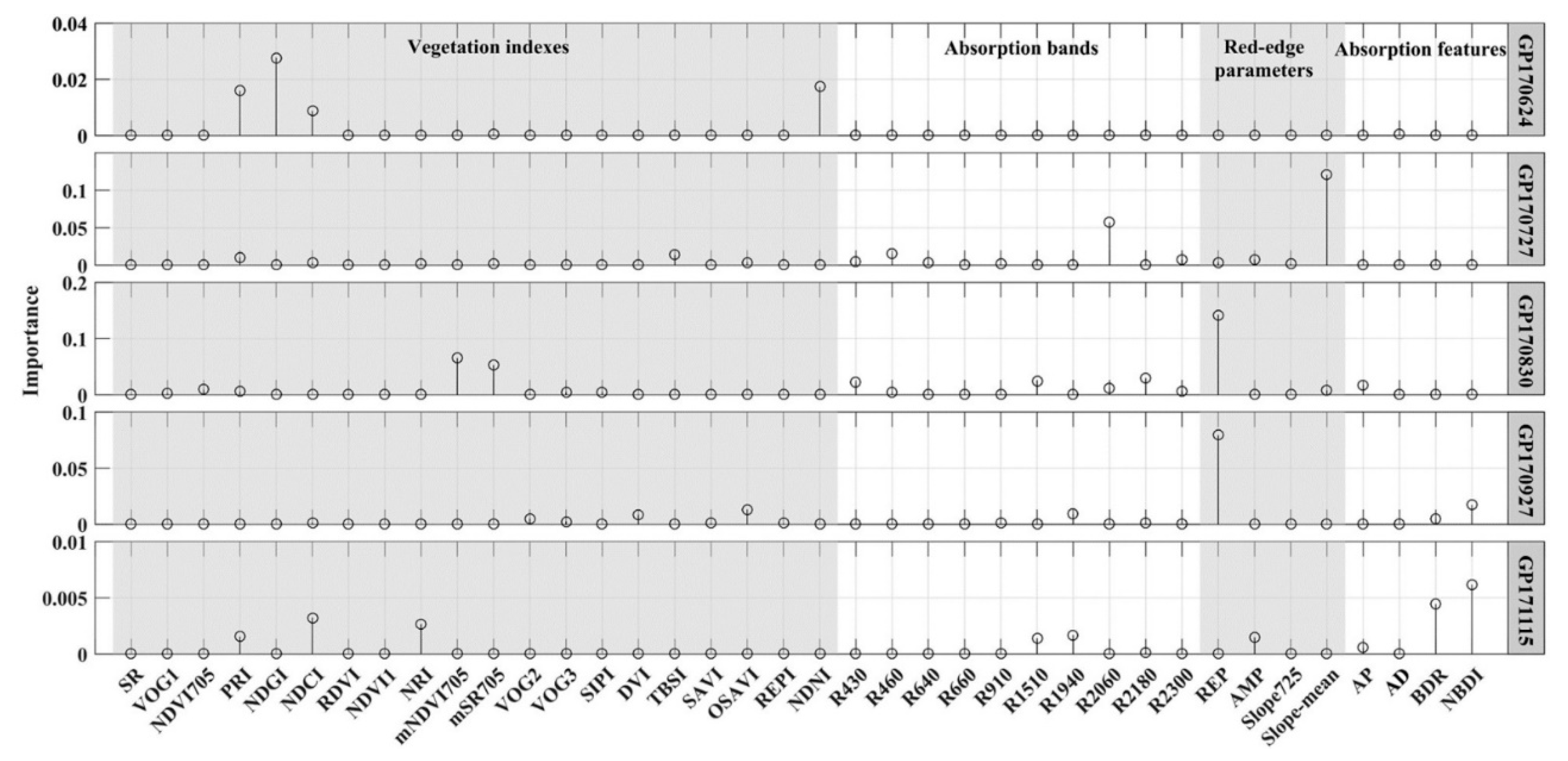
3.4. Estimation Model for Forage N during Different Growth Periods

In this study, the SBS algorithm and V-R2 are employed to determine the optimal variable combinations that have the least number of variables and the best modeling performance for estimating forage N during different growth periods, as shown in Table 3. From GP170624 to GP171115, the number of selected variables ranges from four to six, thus accounting for 10.5–15.8% of all variables, indicating that the variable selection method based on the RF algorithm yields the desired result (the information contained in a few variables can represent the majority of variables). To further evaluate the predictive ability of the N estimation model at different growth periods, we use LOO CV to assess the accuracy of the model, as shown in Table 3. The results show that the N model for the first four periods (GP170624–GP170927) can explain 58–68% of the variance in the forage N content, except for the last period (GP171115), which is only 23%, as shown in Table 3 and Figure 6. The N model yields higher accuracy in GP170624 (V-R2 = 0.68, V-RMSE = 0.2046%, 9.46% of the mean) and GP170830 (V-R2 = 0.67, V-RMSE = 0.2202%, 12.78% of the mean) than in the other periods. The accuracy in GP171115 may be related to the low N content and weak absorption features during the grass senescent period. Overall, the CVRMSE of the model during different growth periods are all less than 20%, indicating that these N models have good predictive capability.

3.5. Estimation Model for Forage N throughout the Growth Periods

To further develop a N estimation model applicable for each growth period, the FFS and four CV strategies (LOO, LTO, LLO, and LLTO) are employed to select feature variables and evaluate the predictive ability of the model to data of unknown growth periods and unknown sample areas, as shown in Table 4. For the whole growth period (entire datasets), the NDVI, PRI, REP, Slope_mean, and R640 are determined to detect variations in forage N. Among the four validation strategies, LOO CV shows a good performance between the measured and simulated data (V-R2 = 0.51, V-RMSE = 0.3741). In addition, the ability of the model to predict the N of the unknown locations (LLO CV) within the four sample areas remains high (V-R2 = 0.55). However, for an unknown growth period (LTO CV) or faced with unknown location and period simultaneously (LLTO CV), the prediction ability of the model is lower than the other validation strategies (V-R2 is 0.28 and 0.29 for LTO CV and LLTO CV, respectively). These findings indicate that the model based on the above five variables and the entire datasets can overcome the spatial differences between different sample areas in the study area; however, predicting the temporal changes of forage N in the unknown growth period is difficult. A significant reason may be that the forage N content varies greatly on a temporal scale (different growth period). The spectral variables available in this study cannot easily capture the variations in N at each growth period, which indicates that the sensitivity of spectral variables to N are not consistent in different growth periods.

4. Discussion

4.1. Variation in Forage N Contents during Different Growth Periods

This study shows that the forage N content presents a gradual decrease with the advancement of the growth period in the alpine grassland (from the end of June to the middle of November), as shown in Table 2. Especially in the latter three periods (GP170830–GP171115), the forage N decreases rapidly. The N content is the highest in GP170624 (2.16%), when it is approximately 2.5 times higher than that in GP171115. Many previous studies have also found that the crude protein of grass in alpine grasslands on the Tibetan Plateau gradually decreases with plant growth, and the content is the highest in June [58,59,60]. These findings also indirectly confirming our result about the variation trend in forage N.
In the present study, the reason for the changes in forage N can be explained by dividing the whole growth period into two stages. The first stage is from the end of June to the end of August (GP170624–GP170830), when grass mainly undergoes vegetative and reproductive growth. As dry matter accumulates in the plant, the biomass also increases, the mechanical tissues of plants grow, and the proportion of physiologically active, nonmechanical tissues declines gradually [61,62]. Because there are large amounts of crude fiber, such as lignin and cellulose but little N in mechanical tissues, crude protein eventually shows a decreasing trend as the forage quantity increase [63]. The second stage is from the end of August to the middle of November (GP170830–GP171115); when the temperature decreases, the frost-free period becomes shorter, and the forage stops growing and begins to senesce. Meanwhile, the resorption of plants has weakened, resulting in the continuous decrease in forage N content [64,65].

4.2. Spectral Characteristics of the Forage Canopy during Different Growth Periods

The spectral reflectance of grassland vegetation is characterized by the canopy morphology and structure, the internal structure of leaves, and the compounds of different components, which are affected by various factors such as water content, chlorophyll content, vegetation coverage, growth period, soil condition, and atmospheric condition [23,24]. In the visible region, the chlorophyll content in leaves is the most important factor that affects the characteristics of leaf reflectance [66,67,68]. Especially in the red-edge region (680–750 nm), the spectral features are closely related to the biochemical parameters, such as N, protein, and chlorophyll [21,31,69,70]. This study has shown that, as the growth period advances, the red-edge first shifts toward longer wavelengths and then toward shorter wavelengths; AMP and AD gradually decrease, and AP changes slightly (most at 678 nm), as shown in Figure 3. In a related study, Zhang et al. also indicated that the REP first shifts to the near-infrared direction then to the green direction from the late stage of returning to green to the vigorous growth period and then to a yellowing and withering period of vegetation [71,72]. The general variation trends of AD and AMP are similar to those observed in this study.
The regular changes in these spectral feature parameters during the growth period can also reflect the growth and development of grassland, which may be related to the morphological changes in vegetation and some physicochemical parameters. For instance, the REP and AMP has a significant relationship with the N content, and the red-edge shift towards longer wavelengths when the N supply increases [31]. For the entire growth period (GP170624–GP171115), the changes of the forage N are similar to that of the spectral features (REP, AMP, and AD) as a whole, as shown in Figure 4; this suggests that the dynamic changes in the spectral feature parameters during different growth periods in the red region may be coupled with the variations in N content. Furthermore, the results of this study also indicated that those features (REP, Slope725, Slope_mean, NBDI, etc.) contribute to the estimation of forage N during different growth periods, as shown in Table 3 and Table 4.

4.3. Applicability of Spectral Variables for Estimating Forage N during Different Growth Periods

The study shows that the importance of the spectral parameters differs during different growth periods, as shown in Figure 5, and the general model of forage N developed with all available datasets has a lower estimation accuracy (LOO CV, V-R2: 0.51 versus V-R2: 0.58–0.68) compared with the single growth period (GP170624–GP170927), as shown in Figure 6 and in Table 3 and Table 4. The reason for this trend may be that the morphological structure and physicochemical characteristics of the plants change significantly as the growth and development of vegetation; thus, the applicability of different spectral parameters will inevitably differ during different growth periods. According to our results, the N model yields higher accuracy in GP170624 (V-R2 = 0.68) and GP170830 (V-R2 = 0.67) than in the other periods. In comparison with the results for estimating the concentration of N by using the reflectance of a tropical grass (Cenchrus ciliaris) (R2 = 0.73) [31], the estimation results of our model are satisfactory. However, most studies only detect forage N content during a particular period without considering changes in different growth periods. This study attempts to estimate forage N content in alpine grassland during different growth stages for covering the shortcoming due to using a single period.
As shown in Figure 6, the model overestimates N at lower levels and underestimates it at higher ones. This may be attributable to the prediction results of RF model, which are determined by multiple decision trees through voting, and the simulation results tend to be the average of the training data. We analyzed the reasons for model results overestimating and underestimating in this study, and found that (1) the small sample size is one of the fundamental reasons for this phenomenon, and (2) the parameters of the RF model and small correlations between predictors also affect overestimation or underestimation of the model. The overestimation is due to the fact that the OOB observations used to derive predictions from the trees might not be representative. Using stratified subsampling for both tuning parameter selection and error estimation in random forests might therefore be a solution to reduce the bias in the estimated value [73]. In addition, the estimation result of the N model shows a large bias in the last period (GP171115), and the phenomenon of overestimation and underestimation is more obvious. This may be caused by the low N content and vegetation coverage of grassland during this period when most variables are less sensitive to forage N. Moreover, bare soil also has a significant influence on N estimates.
During vegetative growth and reproductive growth, the chlorophyll in plants increases and organic matter accumulates continuously. Some spectral variables (i.e., NDNI, VOG, PRI, SIPI, and REP) that are sensitive to chlorophyll and N play a significant role in the estimation of forage N [31,42,74,75], and the N model in the corresponding period also exhibits acceptable estimation accuracy, as shown in Table 3. In addition, when the leaf area index (LAI) of vegetation is very high (i.e., the vegetation is very dense), the sensitivity of SR and NDVI to N will be decreased [31,76,77]. As the plant undergoes senescence, chlorophyll decomposes gradually and the coverage and canopy density decrease rapidly; accordingly, variables that were previously sensitive to N and chlorophyll previously may become insensitive. However, some spectral variables, such as SAVI, OSAVI, BDR, and NBDI, may contribute significantly to the detection of N during this period because SAVI and OSAVI have the potential to effectively eliminate the soil background effect [47,78]; BDR and NBDI are calculated from the continuum-removed spectrum in which the absorption features of forage nutrients are strengthened [8,26]. These results support the findings of this study that the NBDI, OSAVI, and BDR are three of the first five most important variables for N estimation in GP170927, as shown in Table 3. In particular, when the grassland is completely senesced (GP171115), the majority of the spectral variables are no longer sensitive to the weak absorption features of N, which directly results in the unsatisfactory accuracy of the forage N model (V-R2 = 0.23).
According to the preliminary results of this study, multivariate models should be developed for the estimation of forage biochemical parameters during different growth periods in the alpine grasslands. However, developing a spectral variable suitable for estimating forage N in alpine grasslands over the whole growth period is challenging. In subsequent studies, it will be meaningful to focus on estimating the forage N during the grass senescing period while further optimizing the multivariate models during different growth periods.

4.4. Target-Oriented Validation

Our study shows that the predictive performance of the N estimation model based on an unknown growth period is lower than that based on an unknown sample area (V-R2 = 0.28 of LTO CV vs. V-R2 = 0.55 of LLO CV), as shown in Table 4, which indicated that the difference in grassland vegetation at different growth periods is the primary factor restricting the prediction accuracy of the model. The reasons for this finding may related to (1) the considerable variations in the vegetation canopy morphology, biochemical substance concentration, coverage, and height, as well as soil background during different growth periods; and (2) limitations of the available sample size in this study. An ideal RF model relies on the analysis of large amounts of data to establish robust models [27]. Most validation strategies for spatial and temporal models in previous studies are based on random k-fold CV or a random validation subset of the entire dataset [79,80]. However, some studies have concluded that the spatio-temporal machine learning models are prone to temporal or spatial over-fitting and need to be evaluated by LLO CV and LTO CV [56,81]. This study attempted to develop a general forage N estimation model suitable for each growth period using a target-oriented FFS algorithm and validation strategies; however, a low predictive ability was observed for the model based on LTO CV. For this, subsequent studies will need to integrate more sample data and a wider variety of spectral variables to further explore this issue to develop a more practical and applicable forage N estimation model across the whole growth period of alpine grassland.

5. Conclusions

On the basis of the 20 permanent sample plots in four sampling areas and five field observations from the end of June to the middle of November (GP170624–GP171115), this study finds that the changes between the forage N and spectral features (REP, AMP, and AD) are similar throughout the grass growth period. This result indicates that the forage N contents during different growth periods can be estimated based on the aforementioned relationship. Furthermore, the importance of 38 spectral variables for estimating forage N were measured; results show that the applicability of spectral variables are different during different growth periods, indicating that a multivariate forage N estimation model for different growth periods has the potential to improve the stability and accuracy of the results, especially under the background of the large spatial heterogeneity of alpine grasslands.
This study provides insights towards enhancing the universality of forage N models and the sustainable utilization and management of natural alpine grassland resources. However, the result presents an unsatisfactory accuracy (V-R2 = 0.23) when grass is completely senesced (GP171115), possible related to the low N contents and weak absorption features. This result also provides new insights for further developing a novel model for monitoring the forage N content in dead components of grasslands. The grass withering period lasts for five months (from November to March) in alpine grasslands, and the nutrition status of grass greatly affects the growth and reproduction of grazing livestock on the Tibetan Plateau during this period. In addition, four target-oriented validation strategies (LOO CV, LTO CV, LLO CV, and LLTO CV) are applied to assess the predictive performance of the general N model, which is established using all data sets. The results indicate that the difference of grassland vegetation at different growth periods is the primary factor restricting the prediction accuracy of the model. However, it is necessary to verify the predictive ability of spatio-temporal model by using different validation strategies in further studies.

Author Contributions

All authors contributed significantly to this manuscript. J.G. (Jinlong Gao) and T.L. designed this study. J.G. (Jinlong Gao), J.Y., J.G. (Jing Ge), Q.F., C.W., M.H. and J.L. were responsible for the data processing, analysis, and paper writing. H.X. made valuable revisions and editing of the paper.

Funding

This research was funded by the National Natural Science Foundation of China (31672484, 31702175, and 41401472), the Program for Changjiang Scholars and Innovative Research Team in University (IRT_17R50), the National Key Research and Development Program of China project (2017YFC0504801), and the 111 Project (B12002).

Acknowledgments

We acknowledge editors and reviewers for their positive and constructive comments and suggestions.

Conflicts of Interest

All coauthors declare that there is no conflict of interests.

References

  1. He, J.S.; Wang, L.; Flynn, D.F.B.; Wang, X.P.; Ma, W.H.; Fang, J.Y. Leaf nitrogen: Phosphorus stoichiometry across Chinese grassland biomes. Oecologia 2018, 155, 301–310. [Google Scholar] [CrossRef]
  2. Lu, X.; Yan, Y.; Sun, J.; Zhang, X.K.; Chen, Y.C.; Wang, X.D.; Cheng, G.W. Carbon, nitrogen, and phosphorus storage in alpine grassland ecosystems of Tibet: Effects of grazing exclusion. Ecol. Evol. 2015, 5, 4492–4504. [Google Scholar] [CrossRef]
  3. Adams, M.A.; Turnbull, T.L.; Sprent, J.I.; Buchmann, N. Legumes are different: Leaf nitrogen, photosynthesis, and water use efficiency. Proc. Natl. Acad. Sci. USA 2016, 113, 4098–4103. [Google Scholar] [CrossRef] [Green Version]
  4. Heckathorn, S.A.; Delucia, E.H.; Zielinski, R.E. The contribution of drought-related decreases in foliar nitrogen concentration to decreases in photosynthetic capacity during and after drought in prairie grasses. Physiol. Plant. 1997, 101, 173–182. [Google Scholar] [CrossRef]
  5. Lu, J.L.; Hu, A.T. Plant Nutriology; Higher Education Press: Beijing, China, 2006. [Google Scholar]
  6. Reich, P.B.; Walters, M.B.; Tjoelker, M.G.; Vanderklein, D.; Buschena, C. Photosynthesis and respiration rates depend on leaf and root morphology and nitrogen concentration in nine boreal tree species differing in relative growth rate. Funct. Ecol. 2010, 12, 395–405. [Google Scholar] [CrossRef]
  7. Beeri, O.; Phillips, R.; Hendrickson, J.; Frank, A.B.; Kronberg, S. Estimating forage quantity and quality using aerial hyperspectral imagery for northern mixed-grass prairie. Remote Sens. Environ. 2007, 110, 216–225. [Google Scholar] [CrossRef]
  8. Mutanga, O.; Adam, E.; Adjorlolo, C.; Rahman, E.M.A. Evaluating the robustness of models developed from field spectral data in predicting African grass foliar nitrogen concentration using WorldView-2 image as an independent test dataset. Int. J. Appl. Earth Obs. Geoinf. 2015, 34, 178–187. [Google Scholar] [CrossRef]
  9. Mutanga, O.; Skidmore, A.K.; Prins, H.H.T. Predicting in situ pasture quality in the Kruger National Park, South Africa, using continuum-removed absorption features. Remote Sens. Environ. 2004, 89, 393–408. [Google Scholar] [CrossRef]
  10. Singh, L.; Mutanga, O. Remote sensing of key grassland nutrients using hyperspectral techniques in KwaZulu-Natal, South Africa. J. Appl. Remote Sens. 2017, 11, 036005. [Google Scholar] [CrossRef]
  11. Shoko, C.; Mutanga, O.; Dube, T. Progress in the remote sensing of C3 and C4 grass species aboveground biomass over time and space. ISPRS J. Photogramm. Remote Sens. 2016, 120, 13–24. [Google Scholar] [CrossRef]
  12. Adjorlolo, C.; Cho, M.A.; Mutanga, O.; Ismail, R. Optimizing spectral resolutions for the classification of C3 and C4 grass species, using wavelengths of known absorption features. J. Appl. Remote Sens. 2012, 6, 217–224. [Google Scholar] [CrossRef]
  13. Mccann, C.; Repasky, K.S.; Lawrence, R.; Powell, S. Multi-temporal mesoscale hyperspectral data of mixed agricultural and grassland regions for anomaly detection. ISPRS J. Photogramm. Remote Sens. 2017, 131, 121–133. [Google Scholar] [CrossRef]
  14. Ramoelo, A.; Skidmore, A.K.; Cho, M.A.; Mathieu, R.; Heitkönig, I.M.A.; Dudeni-Tlhone, N.; Schlerf, M.; Prins, H.H.T. Non-linear partial least square regression increases the estimation accuracy of grass nitrogen and phosphorus using in situ hyperspectral and environmental data. ISPRS J. Photogramm. Remote Sens. 2013, 82, 27–40. [Google Scholar] [CrossRef]
  15. Ramoelo, A.A. Monitoring grass nutrients and biomass as indicators of rangeland quality and quantity using random forest modelling and WorldView-2 data. Int. J. Appl. Earth Obs. Geoinf. 2015, 43, 43–54. [Google Scholar] [CrossRef]
  16. Curran, P.J. Remote sensing of foliar chemistry. Remote Sens. Environ. 1989, 30, 271–278. [Google Scholar] [CrossRef]
  17. Knox, N. Observing Temporal and Spatial Variability of Forage Quality. Ph.D. Thesis, Faculty Geo-Information Science and Earth Observation and Twente University, Enschede, The Netherlands, 2010. [Google Scholar]
  18. Schlerf, M.; Atzberger, C.; Hill, J.; Buddenbaum, H.; Werner, W.; Schüler, G. Retrieval of chlorophyll and nitrogen in Norway spruce (Picea abies L. Karst.) using imaging spectroscopy. Int. J. Appl. Earth Obs. Geoinf. 2010, 12, 17–26. [Google Scholar] [CrossRef]
  19. Skidmore, A.K.; Ferwerda, J.G.; Mutanga, O.; Van Wieren, S.E.; Peel, M.; Grant, R.C.; Prins, H.H.T.; Balcik, F.B.; Venus, V. Forage quality of savannas–simultaneously mapping foliar protein and polyphenols for trees and grass using hyperspectral imagery. Remote Sens. Environ. 2010, 114, 64–72. [Google Scholar] [CrossRef]
  20. Mutanga, O.; Skidmore, A.K. Red edge shift and biochemical content in grass canopies. ISPRS J. Photogramm. Remote Sens. 2007, 62, 34–42. [Google Scholar] [CrossRef]
  21. Clevers, J.G.P.W.; Gitelson, A.A. Remote estimation of crop and grass chlorophyll and nitrogen content using red-edge bands on Sentinel-2 and -3. Int. J. Appl. Earth Obs. Geoinf. 2013, 23, 344–351. [Google Scholar] [CrossRef]
  22. Lin, D.; Wei, G.; Jian, Y. Application of spectral indices and reflectance spectrum on leaf nitrogen content analysis derived from hyperspectral LiDAR data. Opt. Laser Technol. 2018, 107, 372–379. [Google Scholar]
  23. Choubey, V.K.; Choubey, R. Spectral reflectance, growth and chlorophyll relationships for rice crop in a semi-arid region of India. Water Resour. Manag. 1999, 13, 73–84. [Google Scholar] [CrossRef]
  24. Sims, D.A.; Gamon, J.A. Relationships between leaf pigment content and spectral reflectance across a wide range of species, leaf structures and developmental stages. Remote Sens. Environ. 2002, 81, 337–354. [Google Scholar] [CrossRef]
  25. Ramoelo, A.; Cho, M.A.; Madonsela, S.; Mathieu, R.; Korchove, R.V.D.; Kaszta, Z.; Wolf, E. A potential to monitor nutrients as an indicator of rangeland quality using space borne remote sensing. IOP Conf. Ser. Earth Environ. Sci. 2014, 18, 012094. [Google Scholar] [CrossRef] [Green Version]
  26. Gong, Z.; Kawamura, K.; Ishikawa, N.; Inaba, M.; Alateng, D. Estimation of herbage biomass and nutritive status using band depth features with partial least squares regression in Inner Mongolia grassland, China. Grassl. Sci. 2016, 62, 45–54. [Google Scholar] [CrossRef]
  27. Breiman, L. Random forests. Mach. Learn. 2001, 45, 5–32. [Google Scholar] [CrossRef]
  28. Mutanga, O.; Adam, E.; Cho, M.A. High density biomass estimation for wetland vegetation using WorldView-2 imagery and random forest regression algorithm. Int. J. Appl. Earth Obs. Geoinf. 2012, 18, 399–406. [Google Scholar] [CrossRef]
  29. Singh, L.; Mutanga, O.; Mafongoya, P.; Peerbhay, K.Y. Multispectral mapping of key grassland nutrients in KwaZulu-Natal, South Africa. J. Spat. Sci. 2018, 63, 155–172. [Google Scholar] [CrossRef]
  30. Gao, J.L.; Meng, B.P.; Liang, T.G.; Feng, Q.S.; Ge, J.; Yin, J.P.; Wu, C.X.; Cui, X.; Hou, M.J.; Liu, J.; et al. Modeling alpine grassland forage phosphorus based on hyperspectral remote sensing and a multi-factor machine learning algorithm in the east of Tibetan Plateau, China. ISPRS J. Photogramm. Remote Sens. 2019, 147, 104–117. [Google Scholar] [CrossRef]
  31. Mutanga, O. Hyperspectral Remote Sensing of Tropical Grass Quality and Quantity. Ph.D. Thesis, International Institute for Geoinformation Science and Earth Observation and Wageningen University, Wageningen, The Netherlands, 2004. [Google Scholar]
  32. Horler, D.N.H.; Dockray, M.; Barber, J. The red edge of plant leaf reflectance. Int. J. Remote Sens. 1983, 4, 273–288. [Google Scholar] [CrossRef]
  33. Guo, C.F.; Guo, X.Y. Estimating leaf chlorophyll and nitrogen content of wetland emergent plants using hyperspectral data in the visible domain. Spectrosc. Lett. 2016, 49, 180–187. [Google Scholar] [CrossRef]
  34. Jordan, C.F. Derivation of leaf area index from quality of light on the forest floor. Ecology 1969, 50, 663–666. [Google Scholar] [CrossRef]
  35. Gitelson, A.A.; Merzlyak, M.N. Spectral reflectance changes associated with autumn senescence of Aesculus hippocastanum L. and Acer platanoides L. leaves. Spectral Features and Relation to Chlorophyll Estimation. J. Plant Physiol. 1994, 143, 286–292. [Google Scholar] [CrossRef]
  36. Datt, B. A new reflectance index for remote sensing of chlorophyll content in higher plants: Tests using Eucalyptus leaves. J. Plant Physiol. 1991, 154, 30–36. [Google Scholar] [CrossRef]
  37. Clevers, J.G.P.W. Imaging Spectrometry in Agriculture—Plant Vitality and Yield Indicators Imaging Spectrometry—A Tool for Environmental Observations; Springer: Dordrecht, The Netherlands, 1994; pp. 193–219. [Google Scholar]
  38. Vogelmann, J.E.; Rock, B.N.; Moss, D.M. Red edge spectral measurements from sugar maple leaves. Int. J. Remote Sens. 1993, 14, 1563–1575. [Google Scholar] [CrossRef]
  39. Fourty, T.; Baret, F.; Jacquemoud, S. Leaf optical properties with explicit description of its biochemical composition: Direct and inverse problems. Remote Sens. Environ. 1996, 56, 104–117. [Google Scholar] [CrossRef]
  40. Serrano, L.; Peñuelas, J.; Ustin, S.L. Remote sensing of nitrogen and lignin in Mediterranean vegetation from AVIRIS data: Decomposing biochemical from structural signals. Remote Sens. Environ. 2002, 81, 355–364. [Google Scholar] [CrossRef]
  41. Gamon, J.A.; Penuelas, J.; Field, C.B. A narrow-waveband spectral index that tracks diurnal changes in photosynthetic efficiency. Remote Sens. Environ. 1992, 41, 35–44. [Google Scholar] [CrossRef]
  42. Penuelas, J.; Baret, F.; Filella, I. Semiempirical indexes to assess carotenoids chlorophyll-a ratio from leaf spectral reflectance. Photosynthetica 1995, 31, 221–230. [Google Scholar]
  43. Rondeaux, G.; Steven, M.; Baret, F. Optimization of soil-adjusted vegetation indices. Remote Sens. Environ. 1996, 55, 95–107. [Google Scholar] [CrossRef]
  44. Richardson, A.J.; Wiegand, C.L. Distinguishing vegetation from soil background information (by gray mapping of Landsat MSS data). Photogramm. Eng. Remote Sens. 1997, 43, 1541–1552. [Google Scholar]
  45. Gitelson, A.A.; Merzlyak, M.N. Signature analysis of leaf reflectance spectra: Algorithm development for remote sensing of chlorophyll. J. Plant Physiol. 1996, 148, 494–500. [Google Scholar] [CrossRef]
  46. Marshak, A.; Knyazikhin, Y.; Davis, A.; Wiscombe, W.; Pilewskie, P. Cloud-vegetation interaction: Use of normalized difference cloud index for estimation of cloud optical thickness. Geophys. Res. Lett. 2000, 27, 1695–1698. [Google Scholar] [CrossRef] [Green Version]
  47. Huete, A.R. A soil-adjusted vegetation index (SAVI). Remote Sens. Environ. 1988, 25, 295–309. [Google Scholar] [CrossRef]
  48. Roujean, J.L.; Breon, F.M. Estimating PAR absorbed by vegetation from bidirectional reflectance measurements. Remote Sens. Environ. 1995, 51, 375–384. [Google Scholar] [CrossRef]
  49. Huete, A.; Didan, K.; Miura, T.; Rodriguez, E.P.; Gao, X.; Ferreira, L.G. Overview of the radiometric and biophysical performance of the MODIS vegetation indices. Remote Sens. Environ. 2002, 83, 195–213. [Google Scholar] [CrossRef]
  50. Schleicher, T.D.; Bausch, W.C.; Delgado, J.A.; Ayers, P.D. Evaluation and Refinement of the Nitrogen Reflectance Index (NRI) for Site-Specific Fertilizer Management. In ASAE Annual International Meeting Report; American Society of Agricultural and Biological Engineers: St Joseph, MI, USA, 1998. [Google Scholar]
  51. Tian, Y.C.; Gu, K.J.; Chu, X.; Yao, X.; Cao, W.X.; Zhu, Y. Comparison of different hyperspectral vegetation indices for canopy leaf nitrogen concentration estimation in rice. Plant Soil 2014, 376, 193–209. [Google Scholar] [CrossRef]
  52. Kumar, L.; Schmidt, K.S.; Dury, S.; Skidmore, A.K. Imaging spectroscopy and vegetation science. Imaging Spectrom. Basic Princ. Prospect. Appl. 2001, 4, 111–155. [Google Scholar]
  53. Mutanga, O.; Skidmore, A.K.; Kumar, L.; Ferwerda, J. Estimating tropical pasture quality at canopy level using band depth analysis with continuum removal in the visible domain. Int. J. Remote Sens. 2005, 26, 1093–1108. [Google Scholar] [CrossRef]
  54. Han, Z.Y.; Zhu, X.C.; Fang, X.Y.; Wang, Z.Y.; Wang, L.; Zhao, G.X.; Jiang, Y.M. Hyperspectral estimation of apple tree canopy LAI based on SVM and RF regression. Spectrosc. Spectr. Anal. 2016, 36, 800–805. [Google Scholar]
  55. Lebedev, A.; Westman, E.; Van Westen, G.; Kramberger, M.; Lundervold, A.; Aarsland, D.; Soininen, H.; Kłoszewska, I.; Mecocci, P.; Tsolaki, M. Random Forest ensembles for detection and prediction of Alzheimer’s disease with a good between-cohort robustness. Neuroimage Clin. 2014, 6, 115–125. [Google Scholar] [CrossRef]
  56. Meyer, H.; Reudenbach, C.; Hengl, T.; Katurji, M.; Nauss, T. Improving performance of spatio-temporal machine learning models using forward feature selection and target-oriented validation. Environ. Model. Softw. 2018, 101, 1–9. [Google Scholar] [CrossRef]
  57. Efron, B.; Gong, G. A leisurely look at the bootstrap, the jackknife, and cross-validation. Am. Stat. 1983, 37, 36–48. [Google Scholar]
  58. Zhao, Z.; Wang, A.L.; Ma, H.S.; Song, H.Q. Studies on dynamics monitor and sustainable development in eastern edge of Qinghai-Tibetan alpine grassland (III Seasonal variational dynamics of nutrional contents of the predominant plants on 8 main grassland types). Pratacult. Sci. 2002, 19, 5–9. [Google Scholar]
  59. Liang, J.Y.; Jiao, T.; Wu, J.P.; Gong, X.Y.; Du, W.H.; Liu, H.B.; Xiao, Y.M. The relationship between seasonal forage digestibility and forage nutritive value in different grazing pastures. Acta Pratacult. Sin. 2015, 24, 108–115. [Google Scholar]
  60. Zhou, H.J.; Mao, Z.X.; Huang, D.J.; Fu, H. Analysis on nutritional quality of Elymus nutans among different populations on Qinghai-Tibet Plateau. Pratacult. Sci. 2011, 28, 1198–1202. [Google Scholar]
  61. Niklas, K.J. Plant allometry, leaf nitrogen and phosphorus stoichiometry, and interspecific trends in annual growth rates. Ann. Bot. 2005, 97, 155–163. [Google Scholar] [CrossRef] [PubMed]
  62. Niklas, K.J.; Owens, T.; Reich, P.B.; Cobb, E.D. Nitrogen/phosphorus leaf stoichiometry and the scaling of plant growth. Ecol. Lett. 2005, 8, 636–642. [Google Scholar] [CrossRef]
  63. Shi, Y.; Ma, Y.L.; Ma, W.H.; Liang, C.Z.; Zhao, X.Q.; Fang, J.Y.; He, J.S. Large scale patterns of forage yield and quality across Chinese grasslands. Chin. Sci. Bull. 2013, 58, 1187–1199. [Google Scholar] [CrossRef]
  64. Huang, J.Y.; Zhu, X.G.; Yuan, Z.Y.; Song, S.H.; Li, X.; Li, L.H. Changes in nitrogen resorption traits of six temperate grassland species along a multi-level N addition gradient. Plant Soil 2008, 306, 149–158. [Google Scholar] [CrossRef]
  65. Li, L.; Gao, X.P.; Li, X.Y.; Lin, L.S.; Zeng, F.J.; Gui, D.W.; Lu, Y. Nitrogen (N) and phosphorus (P) resorption of two dominant alpine perennial grass species in response to contrasting N and P availability. Environ. Exp. Bot. 2016, 127, 37–44. [Google Scholar] [CrossRef]
  66. Gitelson, A.A.; Gritz, Y.; Merzlyak, M.N. Relationships between leaf chlorophyll content and spectral reflectance and algorithms for non-destructive chlorophyll assessment in higher plant leaves. J. Plant Physiol. 2003, 160, 271–282. [Google Scholar] [CrossRef] [PubMed]
  67. Feng, W. Monitoring Nitrogen Status and Growth Characters with Hyperspectral Remote Sensing in Wheat. Ph.D. Thesis, Nanjing Agriculture University, Nanjing, China, 2007. [Google Scholar]
  68. Yoder, B.J.; Pettigrew-Crosby, R.E. Predicting nitrogen and chlorophyll content and concentrations from reflectance spectra (400–2500 nm) at leaf and canopy scales. Remote Sens. Environ. 1995, 53, 199–211. [Google Scholar] [CrossRef]
  69. Filella, I.; Penuelas, J. The red edge position and shape as indicators of plant chlorophyll content, biomass and hydric status. Int. J. Remote Sens. 1994, 15, 1459–1470. [Google Scholar] [CrossRef]
  70. Sibanda, M.; Mutanga, O.; Rouget, M. Testing the capabilities of the new WorldView-3 space-borne sensor’s red-edge spectral band in discriminating and mapping complex grassland management treatments. Int. J. Remote Sens. 2017, 38, 1–22. [Google Scholar] [CrossRef]
  71. Zhang, F.L.; Yin, Q.; Kuang, D.B.; Li, F.X.; Zhou, B.R. Analysis of time series spectrum feature parameters derived from dominant natural grasslands in the region around Qinghai lake. Acta Ecol. Sin. 2005, 25, 3155–3160. [Google Scholar]
  72. Zhang, F.L.; Yin, Q.; Kuang, D.B.; Li, F.X.; Zhou, B.R. Analysis of a spectral experiment conducted through the growth period of the main grassland types found in the region around Qinghai Lake. Acta Pratacult. Sin. 2006, 15, 42–47. [Google Scholar]
  73. Janitza, S.; Hornung, R. On the overestimation of random forest’s out-of-bag error. PLoS ONE 2018, 13, e0201904. [Google Scholar] [CrossRef]
  74. Penuelas, J.; Gamon, J.A.; Freeden, A.L.; Merino, J.; Field, C. Reflectance indices associated with physiological changes in nitrogen and water-limited sunflower leaves. Remote Sens. Environ. 1994, 48, 135–146. [Google Scholar] [CrossRef]
  75. Jago, R.A.; Cutler, M.E.J.; Curran, P.J. Estimating canopy chlorophyll concentration from field and airborne spectra. Remote Sens. Environ. 1999, 68, 217–224. [Google Scholar] [CrossRef]
  76. Sellers, P.J. Canopy reflectance, photosynthesis and transpiration. Int. J. Remote Sens. 1985, 6, 1335–1372. [Google Scholar] [CrossRef]
  77. Thenkabail, P.S.; Smith, R.B.; De Pauw, E. Hyperspectral vegetation indices and their relationships with agricultural crop characteristics. Remote Sens. Environ. 2000, 71, 158–182. [Google Scholar] [CrossRef]
  78. Hatfield, J.L.; Prueger, J.H. Value of using different vegetative indices to quantify agricultural crop characteristics at different growth stages under varying management practices. Remote Sens. 2010, 2, 562–578. [Google Scholar] [CrossRef]
  79. Ke, Y.; Im, J.; Park, S.; Gong, H. Downscaling of MODIS one kilometer evapotranspiration using Landsat-8 data and machine learning approaches. Remote Sens. 2016, 8, 215. [Google Scholar] [CrossRef]
  80. Ludwig, A.; Meyer, H.; Nauss, T. Automatic classification of Google Earth images for a larger scale monitoring of bush encroachment in South Africa. Int. J. Appl. Earth Obs. Geoinf. 2016, 50, 89–94. [Google Scholar] [CrossRef]
  81. Gudmundsson, L.; Seneviratne, S.I. Towards observation-based gridded runoff estimates for Europe. Hydrol. Earth Syst. Sci. 2015, 19, 2859–2879. [Google Scholar] [CrossRef] [Green Version]
Figure 1. Study area at the northeastern margin of the Tibetan Plateau, with the four sampling areas (GJ, YLJ, XC, and AZ) from north to south.
Remotesensing 11 02085 g001
Figure 2. Mean canopy reflectance spectra of forage during different growth periods (the bands distributing in 1351–1420 nm, 1801–1930 nm, and 2301–2500 nm are removed because of the effects of the absorption of leaf water and water vapor).
Remotesensing 11 02085 g002
Figure 3. Change rule of the spectrum feature parameters (REP, AMP, AP, and AD) throughout the alpine grassland growth period (June to November). Higher AD values correspond to more obvious absorption features. Each sample area (i.e., AZ, XC, YLJ, and GJ) includes five sample plots. ALL represents all the samples (n = 100).
Remotesensing 11 02085 g003
Figure 4. Changes in the red-edge parameters (REP and AMP) and red region absorption features (AP and AD) in different sampling areas and growth periods. The green dotted line indicates the logarithm fitting models between the N content and corresponding spectrum feature parameters.
Remotesensing 11 02085 g004
Figure 5. Measured importance of spectral variables for estimating the forage N during different growth periods (higher variable importance corresponds to the greater importance of the variable for estimating forage N).
Remotesensing 11 02085 g005
Figure 6. Relationship between the simulated N and observed N during different growth periods (n = 20): (a) GP170624, (b) GP170727, (c) GP170830, (d) GP170927, and (e) GP171115. Both circle size and color refer to the observed N. The red line indicates the linear regression between the simulated and measured data, and the grey area is the 95% confidence level interval.
Remotesensing 11 02085 g006
Table 1. Spectral variables used for estimating forage N.
Variable TypeVariablesFormula and DescriptionReferences
Vegetation indexes (VIs)Simple ratio index (SR) ρ 800 / ρ 670 [34]
Red-edge normalized difference vegetation index (NDVI705) ( ρ 750 ρ 705 ) / ( ρ 750 + ρ 705 ) [35]
Modified red-edge normalized difference vegetation index (mNDVI705) ( ρ 750 ρ 705 ) / ( ρ 750 + ρ 705 2 ρ 445 ) [24,36]
Modified red-edge simple ratio index (mSR705) ( ρ 750 ρ 445 ) / ( ρ 705 ρ 445 ) [24,36]
Red-edge inflection point (REIP) { 700 + 40 [ ( ρ 670 + ρ 780 ) / 2 ρ 700 ] } / [ ( ρ 740 ρ 700 ) ] [37]
Vogelmann red-edge index 1 (VOG1) ρ 740 / ρ 720 [38]
Vogelmann red-edge index 2 (VOG2) ( ρ 734 ρ 747 ) / ( ρ 715 + ρ 726 ) [38]
Vogelmann red-edge index 3 (VOG3) ( ρ 734 ρ 747 ) / ( ρ 715 + ρ 720 ) [38]
Normalized difference nitrogen index (NDNI) [ log ( 1 / ρ 1510 ) log ( 1 / ρ 1680 ) ] / [ log ( 1 / ρ 1510 ) + log ( 1 / ρ 1680 ) ] [39,40]
Photochemical reflectance index (PRI) ( ρ 531 ρ 570 ) / ( ρ 531 + ρ 570 ) [41]
Structure insensitive pigment index (SIPI) ( ρ 800 ρ 445 ) / ( ρ 800 ρ 680 ) .[42]
Optimized soil-adjusted vegetation index (OSAVI) [ ( 1 + 0.16 ) × ( ρ 800 ρ 670 ) ] / ( ρ 800 + ρ 670 + 0.16 ) [43]
Difference vegetation index (DVI) ρ 810 ρ 680 [44]
Normalized difference greenness index (NDGI) ( ρ 750 ρ 550 ) / ( ρ 750 + ρ 550 ) .[45]
Normalized difference cloud index (NDCI) ( ρ 762 ρ 527 ) / ( ρ 762 + ρ 527 ) [46]
Soil-adjusted vegetation index (SAVI) [ ( 1 + L ) × ( ρ 800 ρ 670 ) ] / ( ρ 800 + ρ 670 + L ) , L   = 0.5[47]
Renormalized difference vegetation index (RDVI) ( ρ 800 ρ 670 ) / ( ρ 800 + ρ 670 ) [48]
Normalized difference vegetation index 1 (NDVI 1) ( ρ 900 ρ 660 ) / ( ρ 900 + ρ 660 ) [49]
Nitrogen reflectance index (NRI) ( ρ 560 ρ 670 ) / ( ρ 560 + ρ 670 ) [50]
Three-band spectral index (TBSI) ( ρ 605 ρ 521 ρ 682 ) / ( ρ 605 + ρ 521 + ρ 682 ) [51]
Absorption bandsThe spectral reflectance at λ nm (Rλ)Λ = 430, 460, 640, 660, 910, 1510, 1940, 2060, 2180, 2300[16,52]
Red-edge parametersRed-edge position (REP) AMPWavelength of the red-edge peak (maximum slope position)[31]
Amplitude (AMP)First derivative value at the red-edge peak (maximum slope)
Slope725First derivative value at 725 nm
Slope_meanFirst derivative value obtained from the corresponding mean red-edge position
Absorption featuresAbsorption position (AP)Absorption position[53]
Absorption depth (AD)AD = 1 − R′, R′ = continuum-removed spectra reflectance value
Band depth ratio (BDR)BDR = BD/BDc, BDc = band depth (BD) of band centre, and BD = AD
Normalized band depth index (NBDI)NBDI = (BD − BDc)/(BD + BDc)
Table 2. Variations in forage N contents (%) during different growth periods at the four sites. In the same sample area and growth period, the N content is the average of the corresponding five sample plots.
Sample AreasGP170624GP170727GP170830GP170927GP171115
AZ2.13 ± 0.14 a1.70 ± 0.16 b1.58 ± 0.15 c1.10 ± 0.12 d0.92 ± 0.08 e
XC1.99 ± 0.29 a1.84 ± 0.26 a1.60 ± 0.23 ab1.29 ± 0.27 b0.92 ± 0.26 c
YLJ1.86 ± 0.20 a1.50 ± 0.08 b1.46 ± 0.18 b1.29 ± 0.20 b0.77 ± 0.08 c
GJ2.67 ± 0.04 a2.20 ± 0.15 b2.18 ± 0.16 b1.96 ± 0.30 b0.93 ± 0.12 c
Average2.16 ± 0.171.81 ± 0.161.72 ± 0.161.41 ± 0.220.89 ± 0.14
Coefficient of variation (%)7.718.979.2115.8115.22
Typical photographs of samples Remotesensing 11 02085 i001 Remotesensing 11 02085 i002 Remotesensing 11 02085 i003 Remotesensing 11 02085 i004 Remotesensing 11 02085 i005
Table 3. RF model of the forage N contents during different growth periods. V-RMSE: the RMSE of the validation dataset; V-R2: the R2 of the validation dataset; CVRMSE: the coefficient of variation of the RMSE.
Growth PeriodsSelected Variables (from the Largest to Smallest Importance)CVNumber of VariablesV-R2V-RMSECVRMSE (%)
GP170624NDGI, NDNI, PRI1, NDCILOO40.680.20469.46
GP170727Slope_mean, R2060, R460, TBSILOO40.620.187010.32
GP170830REP, mNDVI705, mSR705, R2180, R1510, R430LOO60.670.220212.78
GP170927REP, NBDI, OSAVI, R1940, BDRLOO50.580.252617.95
GP171115NBDI, BDR, NDCI, NRILOO40.230.134115.12
Table 4. RF model of the forage N contents throughout the growth periods.
Selected VariablesFeature Selection AlgorithmCVMAEV-R2V-RMSE
NDNI, PRI, REP, Slope_mean, R640FFSLOO0.290.510.3741
FFSLTO0.450.280.5412
FFSLLO0.430.550.5114
FFSLLTO0.380.290.4207

