Drone-Borne Hyperspectral and Magnetic Data Integration: Otanmäki Fe-Ti-V Deposit in Finland

Abstract

The technical evolution of unmanned aerial systems (UAS) for mineral exploration advances rapidly. Recent sensor developments and improved UAS performance open new fields for research and applications in geological and geophysical exploration among others. In this study, we introduce an integrated acquisition and processing strategy for drone-borne multi-sensor surveys combining optical remote sensing and magnetic data. We deploy both fixed-wing and multicopter UAS to characterize an outcrop of the Otanmäki Fe-Ti-V deposit in central Finland. The lithology consists mainly of gabbro intrusions hosting ore bodies of magnetite-ilmenite. Large areas of the outcrop are covered by lichen and low vegetation. We use two drone-borne multi- and hyperspectral cameras operating in the visible to near-infrared parts of the electromagnetic spectrum to identify dominant geological features and the extents of ore bodies via iron-indicating proxy minerals. We apply band ratios and unsupervised and supervised image classifications on the spectral data, from which we can map surficial iron-bearing zones. We use two setups with three-axis fluxgate magnetometers deployed both by a fixed-wing and a multi-copter UAS to measure the magnetic field at various flight altitudes (15 m, 40 m, 65 m). The total magnetic intensity (TMI) computed from the individual components is used for further interpretation of ore distribution. We compare to traditional magnetic ground-based survey data to evaluate the UAS-based results. The measured anomalies and spectral data are validated and assigned to the outcropping geology and ore mineralization by performing surface spectroscopy, portable X-ray fluorescence (pXRF), magnetic susceptibility, and traditional geologic mapping. Locations of mineral zones and magnetic anomalies correlate with the established geologic map. The integrated survey strategy allowed a straightforward mapping of ore occurrences. We highlight the efficiency, spatial resolution, and reliability of UAS surveys. Acquisition time of magnetic UAS surveying surpassed ground surveying by a factor of 20 with a comparable resolution. The proposed workflow possibly facilitates surveying, particularly in areas with complicated terrain and of limited accessibility, but highlights the remaining challenges in UAS mapping.

1. Introduction

The demand for raw materials is steadily growing in our technology driven societies. In Europe, industry and businesses depend heavily on direct and indirect raw material imports (metal ores, fossil energy carriers) [1]. The difficulty of providing selected critical raw materials by European producers is increasing—e.g., for rare earth elements [2]—and therefore innovative technologies in exploration and recycling are needed to decrease dependencies on non-domestic imports of raw materials. In this context, we see a high demand for the exploration of new deposits and/or small or less profitable prospects to sustain the need for metallic and raw materials [3,4,5] and therefore inaccessible or formerly non-lucrative mineral deposits are needed [6]. However, mineral exploration in Europe has to fit to our present societal and economic standards, meaning that sustainable, non-invasive, and efficient exploration strategies are required. Following these requirements, exploration in little explored regions can be started with regional survey approaches, e.g., large-scale satellite and regional airborne mapping. For areas and targets identified as potentially prospective, more detailed investigations are usually performed including—e.g., helicopter airborne surveying and extensive field campaigns. Local airborne surveys cover up to hundreds of square kilometers, but require infrastructures such as airports, fuel, and trained personnel. Additionally, the resolution is restricted by wider line spacing and higher flight altitude that limit the detection or characterization of smaller ore bodies and mineralization. Finally, ground based surveying that includes geophysics, drilling, and extensive sampling are applied to obtain detailed knowledge from identified deposits.

In this context, lightweight unmanned aerial systems (UAS) equipped with optical remote sensing and geophysical sensors are particularly attractive to investigate potential deposits in difficult or environmentally sensitive areas. UAS are able to operate autonomously over a given target, are easily deployable, and have short turn-around times for collecting high resolution data-sets with uniform coverage. Their costs are low and their flexibility is high for planning, timing, and logistics compared to a traditional airborne survey. Relevant information is obtained rapidly and the operation requires less personnel with adequate training and flight permissions. UAS user-friendliness increases with the availability of light-weight and durable batteries, open-source autopilots, flight controllers, and means of customization.

However, UAS-based surveying is restricted by national regulations [7] and practical considerations such as safety aspects. In most countries, it is usually possible to operate in visual-line-of-sight (VLOS) and there are weight limits for flight operations. For mineral exploration, UAS systems are therefore mainly attractive for small-to-medium-sized survey areas, limited to some tens of square kilometers, which means that they compete with local-sized airplane and helicopter surveys and may become a complement to ground based surveys [8].

Accordingly, a multitude of UAS applications [9] have emerged over the past five years including mine surveillance [10], slope stability assessment in mining [11], agriculture [12], infrastructure and construction work [13], archaeology [14], forestry [15], disaster monitoring [16], coastal environmental studies [17] and ground water research [18]. Digital elevation models obtained from UAS can deliver resolutions in (sub-)centimeter range, and are superior to conventional mapping techniques in terms of survey area, time, and target accessibility [19,20].

Hyper- and multispectral cameras are sensors that are frequently used on UAS, although their application has mostly been limited to agriculture. UAS use for mineral mapping is still underrepresented in scientific literature, but recent studies show great potential [21]. Example studies apply UAS, or a combination of UAS and terrestrial scans to identify lithological structures and map lithologic domains [22,23].

For geophysical applications, UAS-based magnetics is attractive since recent sensors are rugged and lightweight [24]. Acquisition and processing strategies from conventional airborne measurements can be adapted for UAS surveys.

Recent studies highlight the potential of UAS to locate man-made ferrous bodies superficially buried in soil having sizes and weights that reflect the properties of unexploded ordnance (UXO) [25] and to map shallow volcano-related structures and magma bodies [26], using combustion-engine UAS helicopters with optically-pumped magnetometers.

Promising mapping results show the potential of multicopter UAS to perform on par with traditional aeromagnetics [27,28]. The used optical pumped magnetometers were suspended on cables below the UAS. The influence of orientation changes for such magnetometer mountings was investigated [29] and resulted in attitude recommendations.

In contrast to UAS heli- and multicopter, autonomous fixed-wings provide the design suitable for long-range magnetic surveys of even larger areas [30].

Although applications of single sensors become more common and the techniques more well-developed, we observe a lack of combining separate survey techniques and, hence, to gain the full geoscientific information simultaneously. The main objective of our study is thus to evaluate the potential of integrated UAS-based remote sensing and geophysical techniques for mineral exploration. We compare those fast and effective survey strategies to traditional ground survey methods in the Otanmäki Fe-Ti-V deposit in Central Finland. We combine UAS-based data including multi- and hyperspectral remote sensing, magnetics, and structure-from-motion multi-vision stereo (SfM-MVS) photogrammetry, to create value for UAS methods in geology.

More specifically for the iron ore deposit in Otanmäki, the motivation of this work is to map iron ore distributions and evaluate ore prospectivity. We chose those UAS-borne sensor types because (1) magnetic field variations are predominantly caused by changing (induced and permanent) magnetization of the iron ore, thus, magnetics is well-suited to determine the distribution of ore lenses and grade estimation; (2) multi- and hyperspectral imaging allows to map surficial alteration of iron minerals in the visible (VIS) and near-infrared (NIR) range of the electromagnetic spectrum. However, magnetite and ilmenite as the main ore minerals in Otanmäki are spectrally featureless in VIS-NIR. Therefore, the objective of this study is to investigate how far it is possible to locate those using proxy minerals, e.g., hematite. The combination of both methods is relevant, because the magnetic anomalies are predominantly caused by magnetite and accordingly, complementary information is collected from magnetic data not obtainable from hyperspectral data. Besides, magnetic measurements from UAS have limited spatial resolution and therefore hyperspectral data can help to more precisely assign anomalies to specific ore lenses or geologic units.

We use both fixed-wing and multicopter UAS for surveying because (1) multicopter allow for controlled low altitude flights with high-resolution sensors; and (2) fixed-wing UAS can quickly map larger areas with light-weight equipment. For ground validation of the UAS results, we conducted a ground magnetic survey, in-situ measurements including spectroscopy, determination of magnetic susceptibility, and laboratory investigations. With ground truthing, we verify the remote sensing results and are able to give accuracy assessments of different techniques. Finally, we point out difficulties for surveying that arise from external conditions, e.g., weather conditions and surface obstructions.

2. Location and Geology

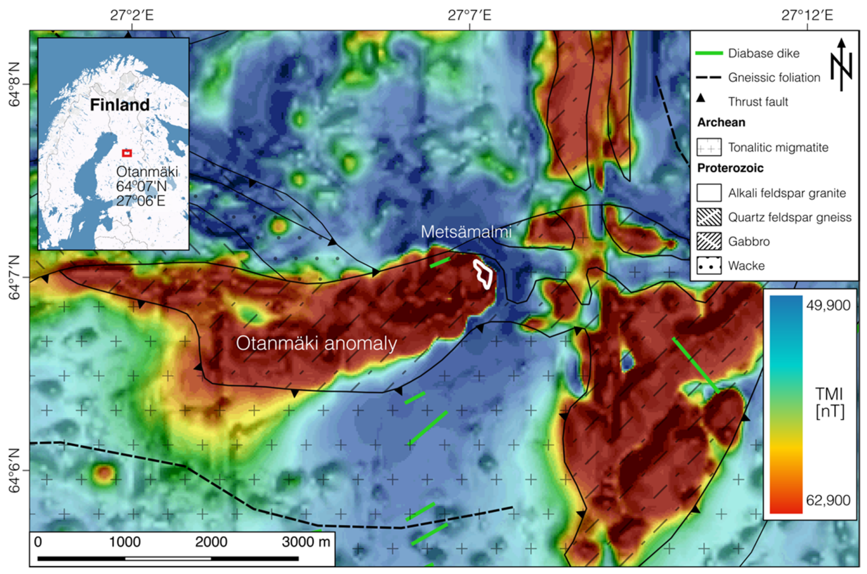
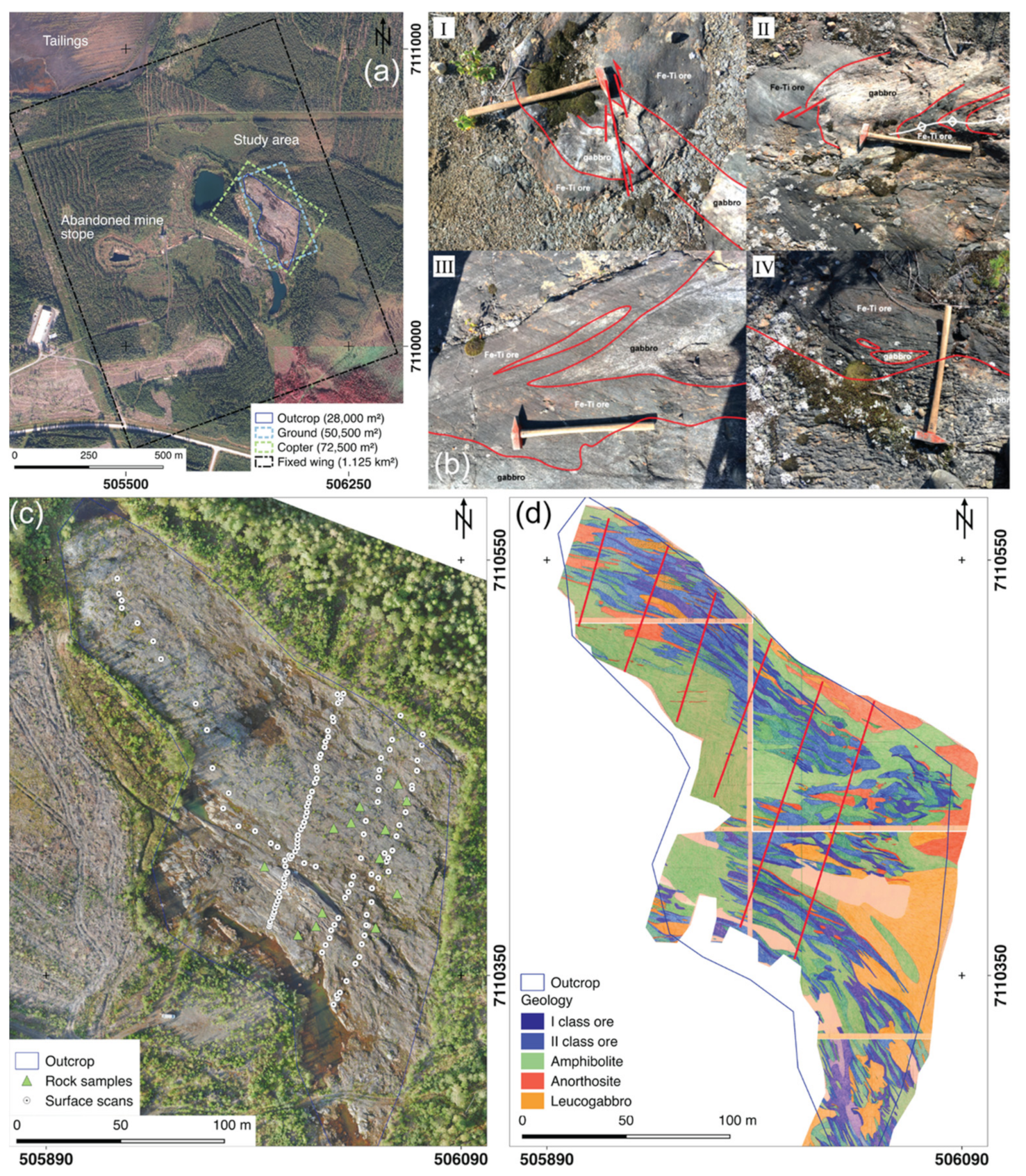
2.1. Regional Setting and Description of the Study Area

The study area is located on the premise of the former Otanmäki Fe-Ti-V mine in central Finland, about 200 km southeast of the city Oulu (Figure 1).

The main target is the exposed Metsämalmi (‘wood ore’ in Finnish) outcrop that is situated on the eastern edge of a large magnetic anomaly (Figure 1). The anomaly is associated with the Otanmäki gabbroic intrusion hosting the magnetite-ilmenite ore deposit [32]. The outcrop has a size of about 28,000 m² and is located in a birch tree forest (Figure 2a). Much of its barren rock surface consists of high-grade ore lenses (see photographs from high-grade ore bodies and detailed geological map in Figure 2b,c, respectively) and it was cleared in the early 1980s for possible open pit mining. However, the decision to close the Otanmäki mine was made shortly afterwards and the Metsämalmi area was left unmined. Large spots (hand-size) of lichen cover its rock surfaces, and an area in the central part of about 30 × 10 m was cleaned up with a high-pressure cleaner some days before the surveys to improve the conditions for hyperspectral surveying.

Apart from the Metsämalmi outcrop, the bedrock in the Otanmäki area is poorly exposed and rocks are largely covered by glacial overburden with a thickness of 1–3 m. Therefore, geophysical surveys play an important role in regional studies to understand the hard rock geology (e.g., originally, the Fe-Ti-V ores were discovered by magnetic measurements). One example is the low-altitude airborne regional magnetic survey from 1979 that was collected within the national airborne geophysical program (see [31]). This survey uniformly covers the complete Otanmäki area (Figure 1) and was flown on an average flight altitude of 37 m and with a (in-)line spacing of 200 m, with lines oriented in N–S direction.

2.2. Geologic Setting

The vanadiferous magnetite-ilmenite ore deposits in the Otanmäki area are located within 2.06 Ga old gabbroic intrusions, which hosts ore within areas (Figure 2b) composed of metamorphosed gabbro, leucogabbro-anorthosite, and lensoidal bodies of massive/semi-massive oxide ore [33,34]. The intrusions were emplaced into Archaean migmatitic tonalite-trondhjemite-granodiorite-gneisses, but they also have sharp, fault defined contacts against gneissic 2.05 Ga old, A-type granites, and intermediate rocks (Otanmäki suite), hosting some Nb-Zr-REE mineralizations. The southern border of the anomaly is a thrust fault line.

The magnetite-ilmenite ore bodies in the Otanmäki gabbro intrusion are scattered within a 50–200 m wide and approximately 5 km long ore-bearing zone having numerous unequally sized and irregularly shaped ore lenses. The ore lenses within this zone are typically sub-vertical, 2–200 m long and 3–50 m thick, generally EW-trending and dipping N at 70–90° [33]. In addition, the rocks in the ore zone are typically pervasively recrystallized and deformed, and the ore zone is folded into a syncline structure at its eastern end. The synform plunges to SW at about 40–60° and the ore zone descents along the fold axis. Based on drilling, the ore zone is known to extend down to a depth of 800 m and gravity-based modeling suggests continuation of the intrusion down to a depth of 2 km [33,35].

The average modal mineralogy of the Otanmäki high-grade ore is composed of magnetite (35–40%), ilmenite (25–30%), and sulphides (1–2%) [36]. Ore types are divided into three classes depending on their Fe-oxide mineral content.

Class I ore has a magnetite and ilmenite content of more than 50 wt %. Main gangue are silicate minerals such as chlorite, hornblende and plagioclase. Sulphide minerals (pyrite, chalcopyrite, and pyrrhotite) can make up to 20% of host rocks and ore. The distribution of mapped class I and II ore lenses in the Metsämalmi outcrop area is shown in Figure 2d. Due to the correlation between ore grade (iron content) and the amount of magnetite, the mining company considered magnetic susceptibility measurements as cost saving technique to estimate the ore.

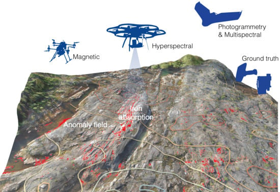
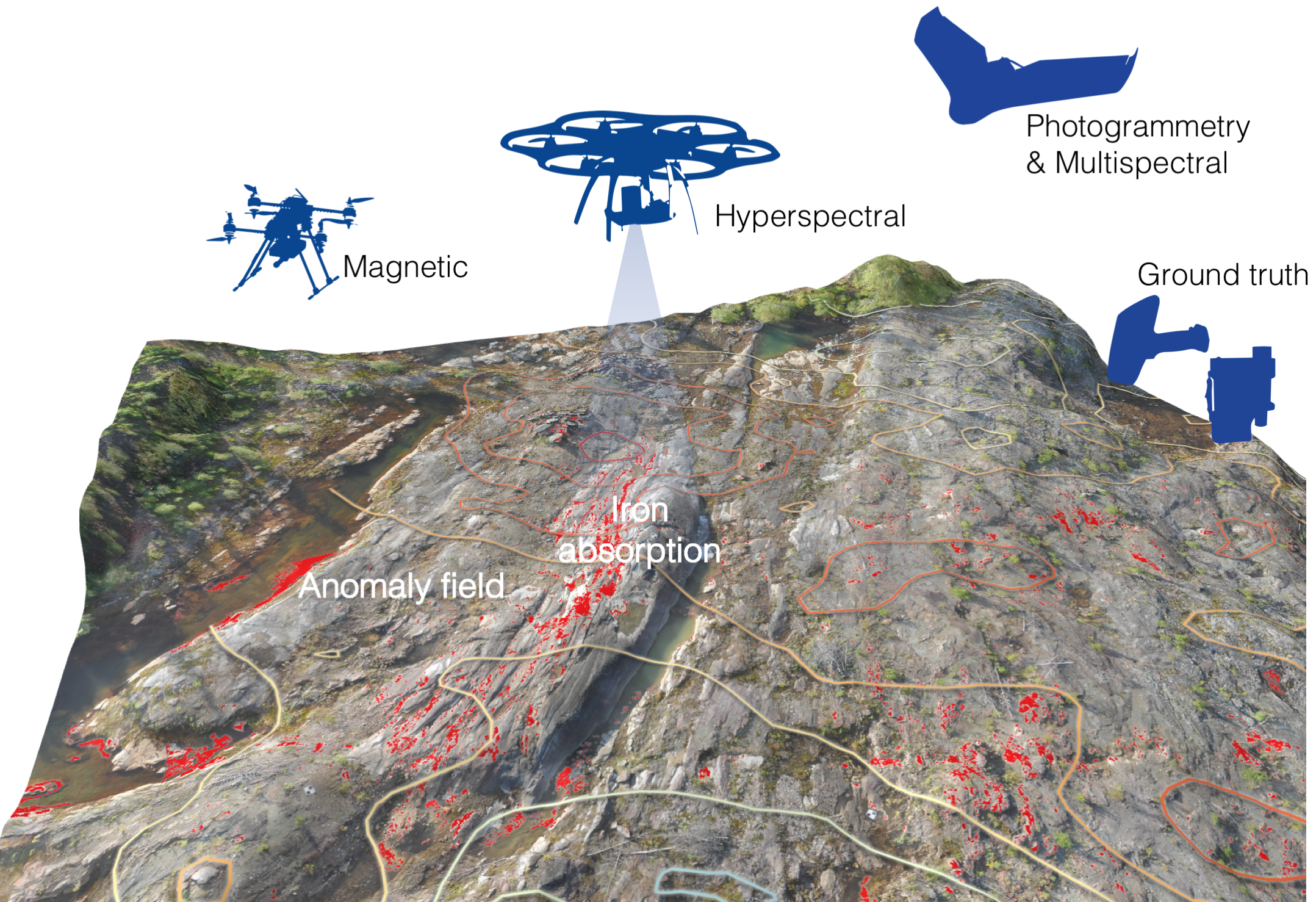
3. Methods and Survey Strategies

We describe the different UAS-based technologies that were used in the field campaign, as well as the acquisition strategies and the workflows to acquire and process the different datasets. For the different UAS, we introduce the platforms and employed sensors and define technical details. The sensors on the multicopters, i.e., magnetometer and frame-based hyperspectral camera are exchangeable within a few minutes. The reasons for this are two-fold: on one hand, the different sensors require different acquisition strategies (e.g., stop-and-go for hyperspectral imaging vs. continuous for magnetics). On the other hand, take-off weight is reduced, resulting in longer flight duration.

3.1. Survey Outline

Figure 3 shows photographs from different UAS types that were used in this field campaign, and their technical parameters and specifications are given in

Table 1. Technical details of the used UAS. The eBee plus instrument is not shown in Figure 3.

Model	Tholeg Tho-R-PX8-12	Aibotix Aibot X6v.2	SenseFly Ebee Plus	Radai Albatros VT
Type	Multicopter	Multicopter	Fixed-wing	Fixed-wing
Rotors	8	6	1	1
MTOW *	10 kg	7 kg	1.1 kg	5 kg
Size	70 × 70 × 35 cm	105 × 105 × 45 cm	110 cm wingspan	2.8 m wingspan
Flight time	20–25 min	12–15 min	59 min	180 min
Velocity	0–40 km/h	0–30 km/h	40–110 km/h	50–110 km/h
Payload	4.5 kg	2 kg	~0.2 kg	2 kg
Sensor	Fluxgate magnetometer	Rikola HSI camera	RGB camera, 4 band multispectral camera	Fluxgate magnetometer

* Maximum take-off weight.

. Data acquisitions with all sensors and UAS types follow along pre-programmed survey patterns based on GPS points, but starts and landings are done manually. We performed ground (Figure 2c) and UAS surveys over the course of three days in September 2018. Weather conditions were favorable with mild temperatures, little cloud coverage, weak wind (~3–7 km/h) and scarce gusts. The flight altitudes are given above ground level (AGL), and range between 15–65 m AGL.

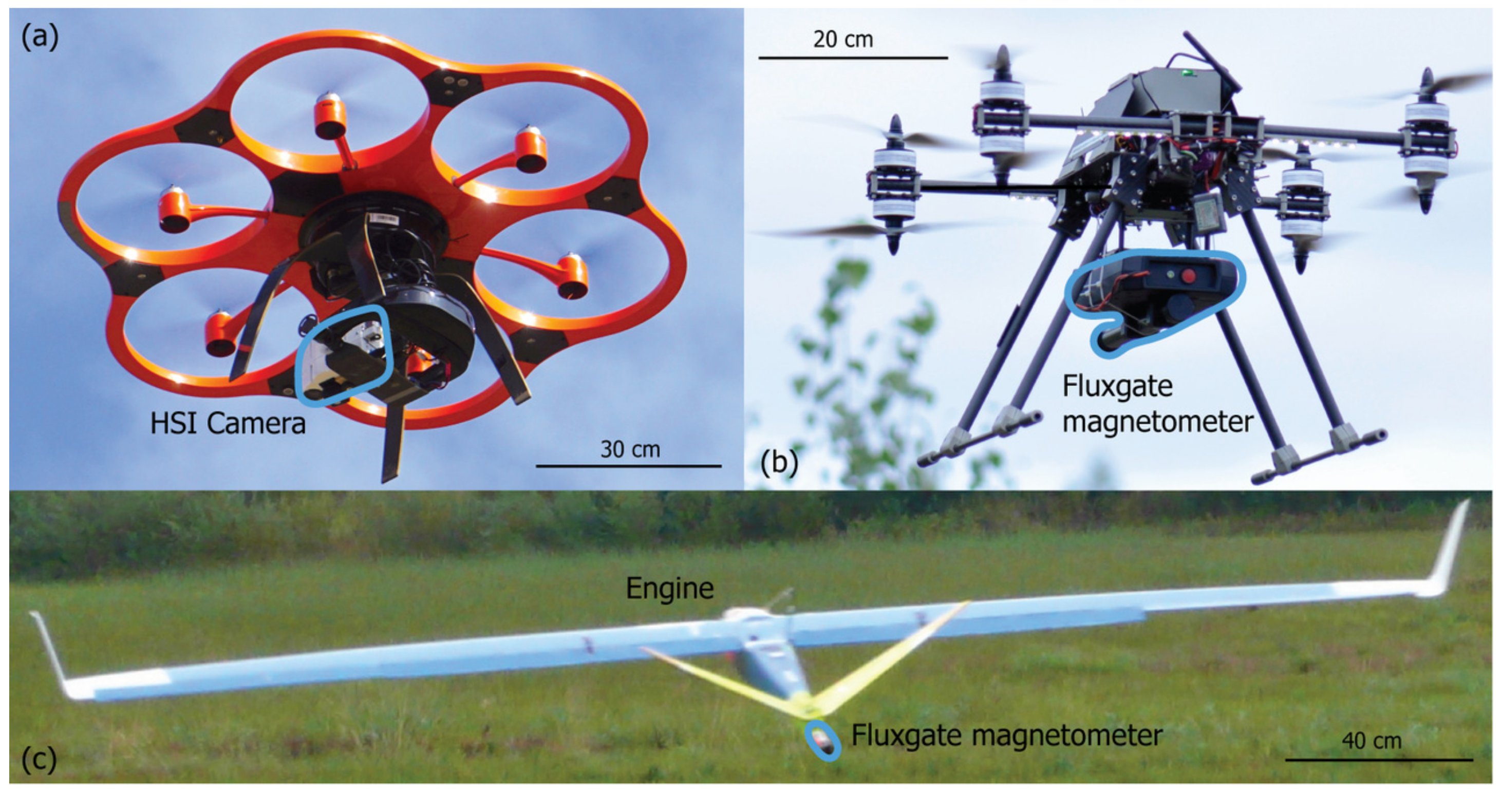
3.2. Multispectral UAS Imaging

We conducted multispectral imaging (MSI) with a Sensefly ebee Plus fixed-wing UAS. The ebee Plus is equipped with the lightweight Parrot Sequoia (1.2 Mpix) four channel multispectral global shutter camera. Its multispectral bands are centred at 550 ± 40 nm (green), 660 ± 40 nm (red), 735 ± 10 nm (red-edge), and 790 ± 40 nm (NIR). Automatic radiometric calibration was performed prior to the flight using a synthetic reference panel provided by the manufacturer. The UAS captured 98 multispectral scenes at 84 m AGL along the programmed flight path, in order to ensure sufficient image overlap. The orthomosaic was processed in Agisoft Photoscan, using optimized multispectral processing option and protocols [37], with the green band as master band. Processing parameters for the image alignment were set to ‘high quality’, while the key point and tie point limit was set to 40,000 and 4,000, respectively, and used with reference preselection. Outlier tie points were removed manually using the gradual selection tool prior to dense image matching (maximum reprojection root mean square error (RMSE) achieved: 0.2 or 3.16 pixel; mean RMSE: 0.1 or 0.39 pixel) followed by optimization of the bundle adjustment. Based on the resulting dense point cloud, an orthomosaic was generated with a ground resolution of 7.4 cm/pixel. Due to low sun elevation in the northern hemisphere (sun altitude 25°; azimuth 228° at 16:00 local time) and late time of the day during data acquisition, we applied a topographic correction using the c-factor correction using the Python based Mephysto image processing toolbox [38].

3.3. Hyperspectral UAS Imaging

Hyperspectral UAS-borne data are captured with the Senops Rikola Hyperspectral Imager. This snapshot sensor has the advantage of acquiring full frame data for up to 50 spectral bands, thus having high frame coherence towards each other with the UAS flying along a stop-and-go data acquisition plan at 30 m altitude AGL.

Table 2. Technical data and settings of the Rikola camera during flight operation.

Parameter	Value
Image Resolution	1010 × 648 Pixel
Bands	50
Spectral range	504–900 nm
Spatial/Spectral resolution	3 cm/8 nm
FWHM	~14 nm
Band integration time	10–50 ms (depending on illumination)
Focal length	9 mm
F-number	2.8
Weight	720 g

lists the camera parameters used for the survey [39].

Pre-processing of the HSI data was again performed with the Mephysto toolbox [38]. Images are co-registered, corrected for geometric effects (lens- and topographic correction) and georeferenced to the RGB orthophoto acquired by SfM-MVS (see Section 3.4). We used the empirical line method for radiometric conversion from radiance to reflectance [40]. For the calibration, we used three PVC reference panels (shades of black, grey, and white) with known spectral signatures. As the HSI scenes generally showed low reflectance, calibration with the grey panel gave satisfying image contrast. As for the multispectral survey, main factor to be corrected is the low sun azimuth. We removed in-scene vegetation using a NDVI-mask (normalized difference vegetation index), [41] for both the multi- and hyperspectral mosaics with a threshold of > 0.3. Smaller water bodies were removed manually. On the masked data, we applied a minimum noise fraction (MNF, [42]) transformation for dimensionality reduction and noise filtering. Subsequently, we applied a k-means [43] unsupervised clustering, with the first 20 MNF bands as input [44]. The number of k-means target classes was determined based on prior field observations. We concluded, that six classes are suitable to account for the different surface features (gabbro, iron-bearing minerals, water, remaining vegetation, soil-debris, noise) and are used for the final output.

Band ratios were used to determine the positions and potential absorption depths for the broad iron absorption feature in hyper- and multispectral imagery and handheld scans. We used the band position for the iron feature at ~900 nm and band reflectance peaks between 750–760 nm, as those positions are as relevant in our application as, e.g., the curve shape [45]. The broad spectral iron feature is caused by a charge-transfer absorption that is diagnostic for iron-bearing minerals [46].

Finally, supervised spectral classification is applied on the processed HSI by using the spectral angle mapper [44]. SAM measures the similarity between a reference and an image spectrum by computing the angle between spectra in an n-dimensional (n = bands) space. Small angles between spectra do indicate high material similarity. Previous studies showed that the SAM technique is well-suited for hyperspectral images featuring of iron-bearing mineralogy [22].

Our experiences with iron-related spectra show that spectral smoothing on the input HSI with a Savitzky-Golay filter [47] of second order and a filter width of 3–5 points (depends on input spectral resolution) increases the accuracy of SAM classifications by removing spectral noise [48].

We used the following samples taken from the USGS library [49] for classification:

• Hematite GDS27 (alpha-Fe₂O₃ – pure hematite) → proxy for iron-oxides [50]
• Goethite WS222 (FeOOH – polymorphous with akaganeite, feroxyhyte, and lepidocrocite) → proxy for iron oxide-hydroxide
• Jarosite GDS 99 Ky200C Syn (KFe⁺³₃(SO4)₂(OH)₆ – synthetic) → proxy for iron-sulphates

These spectral signatures are chosen as proxies for the expected minerals that categorize the major iron bearing groups [33]. Spectral angles from 0.10–0.15 rad using 0.01 rad step-size were applied to achieve the resulting supervised classification. The resulting classes are sieved with a four-pixel neighbourhood kernel to reduce secluded pixels, assuming the maps spatial accuracy is high.

3.4. Structure-from-Motion Multi-Vision Stereo Photogrammetry

Orthophotos and digital surface models (DSM) of the Metsämalmi outcrops were created by drone-borne SfM-MVS photogrammetry. The DSM can be used to correct for altitude variations of magnetic data and illumination effects in the hyperspectral data while the orthophoto is used to geo-reference the HSI. Moreover, the orthomosaic is valuable to understand geologic structures and serves as a reference image for ground sampling points.

We used the Sensefly ebee Plus UAS featuring a 20 MPix S.O.D.A. RGB camera for acquisition of nadir images (technical details in

Table 3. Acquisition parameters of the created orthophoto and DSM from two cameras.

	SODA	Sequoia
Images/Altitude	241/103 m AGL	98/84 m AGL
Orthophoto/DSM–Ground pixel resolutions	2.2 cm/4.3 cm	7.4 cm/-
GCPs number/Mean GCP RMSE	12/8.1 cm	11/43.8 cm

). Image overlap was set to 80% forward and 70% sideways. In total, 12 ground control points were distributed on the outcrop, to precisely geo-reference the final photogrammetric model.

Again, we performed the SfM-MVS workflow using Agisoft PhotoScan following protocols recommended [37,51]. Processing parameters for the image alignment were set to ‘high quality’ and we choose the reference preselection option. Outlier tie points were subsequently removed using the gradual selection tool prior to the dense image matching. We removed tie points detected in less than three images and set a maximum threshold for image re-projection errors to 0.5 (41.69 pixels), to only use tie points below that value for dense cloud matching. The dense image matching or point cloud construction was run at ‘high quality’ with the depth filtering set to ‘aggressive’. The accuracy of the SfM-MVS point cloud was validated based on the measured GCP (ground control points) versus estimated GCP positions in Agisoft PhotoScan. The DSM is computed with an average grid spacing of 4.3 cm/pixel. Finally, an orthophoto with a resolution of 2.2 cm/pixel is computed by seamlessly merging overlapping images. The TecGEMS toolbox [52] is used to automatically extract structural information such as lineaments, ridges, and discontinuities from the DSM. The lineaments were validated with field observations (see Figure 2b).

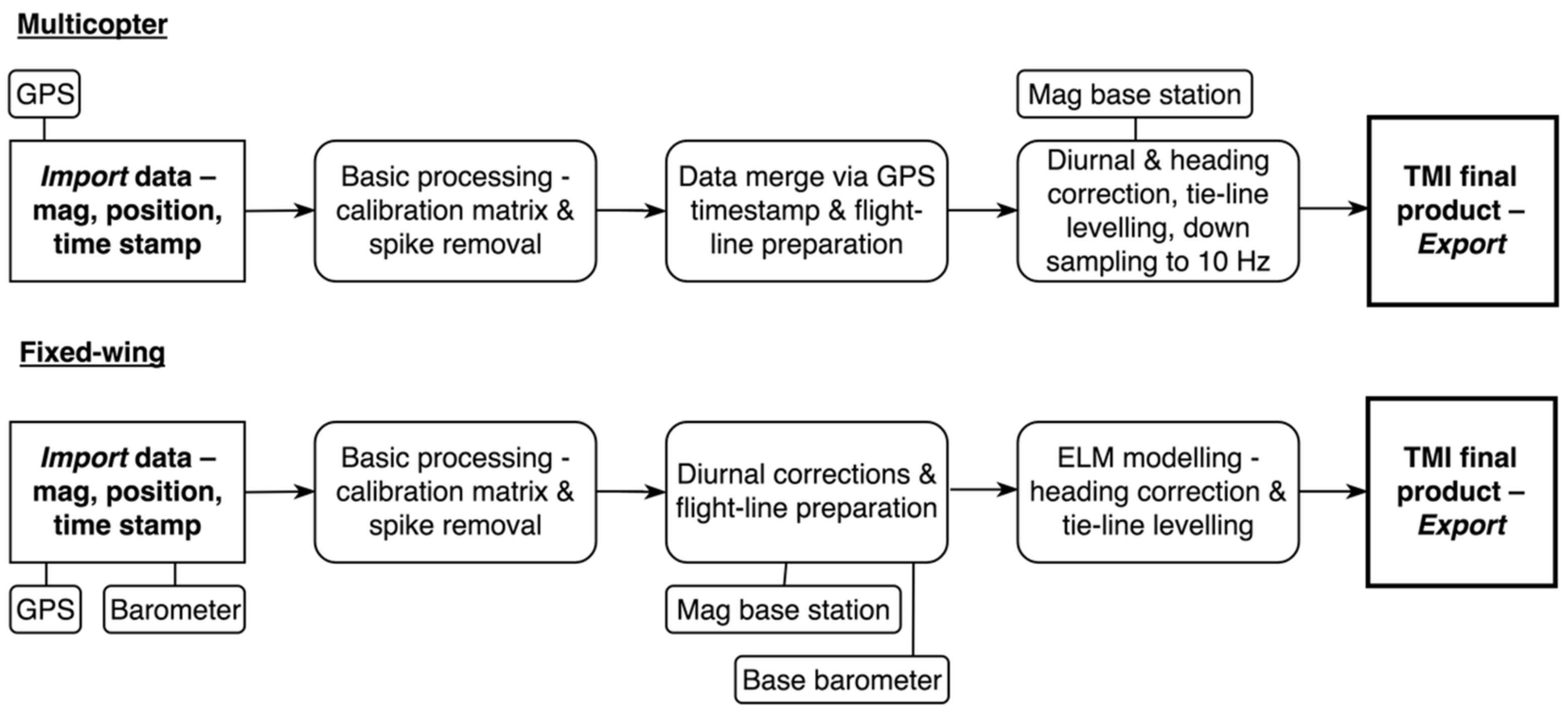
3.5. Copter-Borne Magnetic Measurements

For magnetic measurements with the multicopter we applied a calibrated triaxial fluxgate magnetometer (MagDrone R1; SenSys [53]). It measures the magnetic flux density within a range of ± 75,000 nT and features a sampling frequency of 200 Hz. Further parameters of the magnetometer are given in

Table 4. Parameters of SenSys MagDrone R1 UAS-borne fluxgate magnetometer system [53].

Parameter	Value
Resolution	>0.15 nT
Baseline error (200 Hz sampling)	<4 nT
Fluxgate axes declination	≤±0.5º
Weight	800 g

. The autonomous system can measure up to 2 hours and records GPS data (latitude, longitude, altitude, GPS time) at 20 Hz intervals. Magnetic measurements are interpolated onto coordinate points using GPS time stamps. Recorded data are saved on an internal solid-state memory module.

The MagDrone is rigidly attached below the UAS centre (Figure 3a). The axes of the magnetometer are aligned parallel and perpendicular to the main axis of the UAS fuselage, in a distance of 50 cm to the engines.

During automated flight operation with an average velocity of 5 m/s sampling point inline distance is ~0.5 m. The drone followed a pre-defined flight plan. We performed surveys at different flight altitudes to investigate following applications:

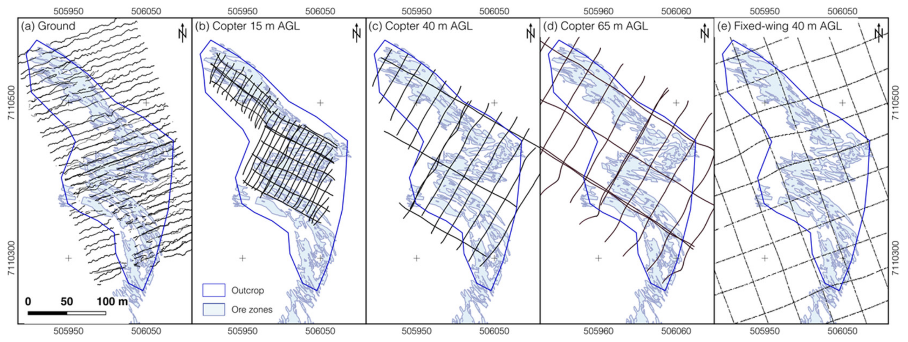
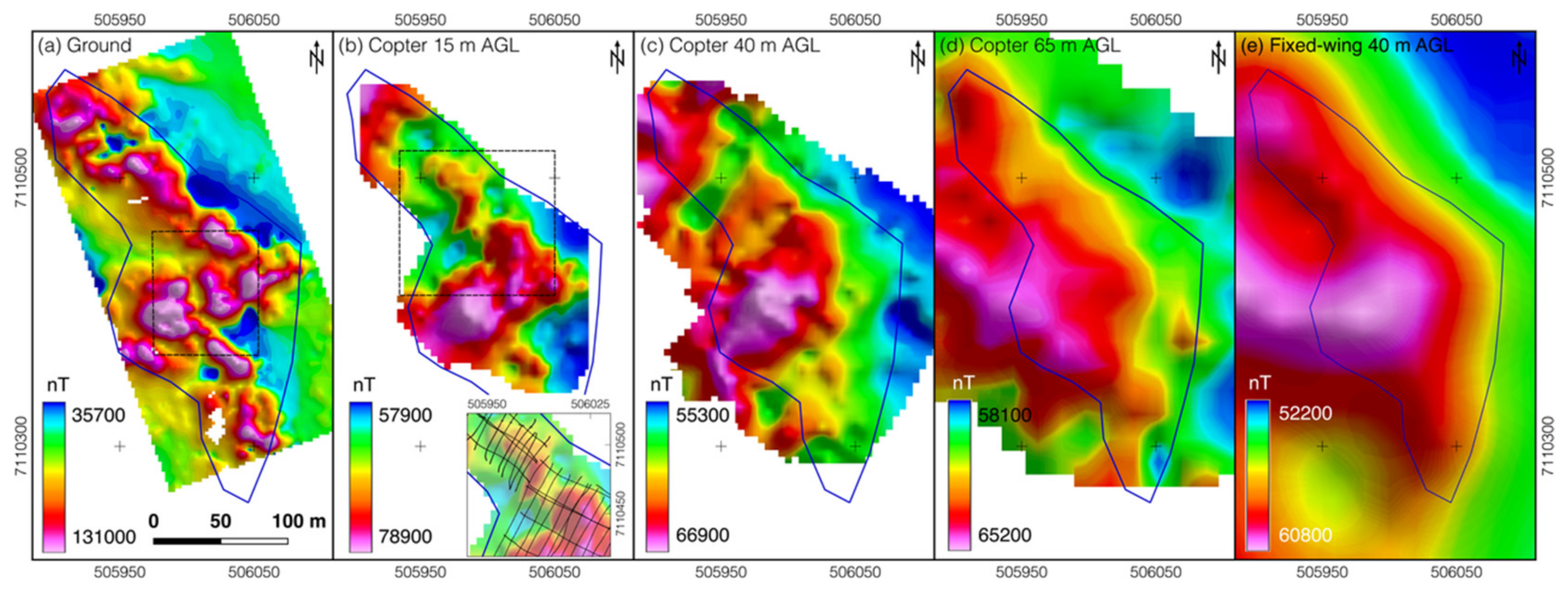
• 15 m: Collect a UAS magnetic dataset close to surface, but within acceptable flight safety margins, for dense spatial coverage approaching the resolution of ground magnetics.
• 40 m: Compare multicopter and fixed-wing data at similar operation height.
• 65 m: Perform high altitude UAS survey to examine the regional behaviour of the anomaly and to have a dataset that can serve as a reference for upward continuations of the other datasets.

Acquisition parameters and results for the surveys at three flight heights are summarized in

Table 5. Parameters of the magnetic surveys. Survey time includes take-off and landing.

Method	Area	Survey Length	Height AGL	Survey Time	Speed	Inline/Tie-Line Spacing
Ground Survey	50,500 m2	9.5 km	1.7 m	3 days	~0.1 m/s	10/- m
Multicopter *	19,000 m2	4.1 km	15 m	32 min	5 m/s	7/20 m
Multicopter	37,000 m2	3.2 km	40 m	19 min	5 m/s	20/80 m
Multicopter	72,500 m2	3.7 km	65 m	25 min	5 m/s	35/60 m
Fixed-wing	1.14 km2	69.6 km	40 m	57 min	20 m/s	40/40 m

* two flights.

. We conducted a calibration flight, using cardinal and inter-cardinal directions, at the beginning of each survey, within altitudes of 30–40 m AGL, to obtain proper heading corrections for each flight line [54]. Further processing steps are given in Figure 4.

During the 15 m survey (Figure 5b), the z-component of the MagDrone magnetometer was saturated for about 1% of the collected magnetic data points. Also, the strong magnetic anomaly disturbed the orientation of the compass used for UAS navigation such that the multicopter flight lines (Figure 5) show some deviations from the original flight plan.

To account for the diurnal variations, a magnetic base station (SenSys MagBase) was set up. It was located with a distance of several hundred meters outside of the high magnetic anomaly to avoid that the changes of the induced magnetic field related to the outer field variations have a measurable impact on the recordings. The total field Bt is computed and its variation is used to correct the drone-borne magnetic total field data. The calculated IGRF (International Geomagnetic Reference Field), considered as the background in the area at the time given, was about 53,056 nT (Declination: 11.3°; Inclination: 75.8°).

During processing, we applied a fluxgate offset calibration matrix (provided by the manufacturer) for MagDrone and MagBase data to account for non-orthogonality between the individual field components. In general, the data processing workflow follows standard protocols for airborne magnetic measurements (e.g., [55]).

3.6. Fixed-Wing Magnetic Measurements

Fixed-wing UAS magnetic measurements were conducted with the Albatros VT UAS, shown in Figure 3c. Survey objective was to capture data on a kilometer scale with dense line spacing and therefore high resolution. The magnetic field is measured by a digital triaxial fluxgate magnetometer that is located in the tail boom of the UAS. The components of the magnetic field, the GPS position and time, and barometric pressure are recorded by the datalogger.

After manual take-off, the UAS flight is controlled by an autopilot software and follows predefined waypoints over the eastern part of the Otanmäki deposit, including the Metsämalmi outcrop. The UAS follows the terrain topography based on a 10 × 10 m DSM grid provided by the National Land Survey of Finland. The flight performance is controlled online both via a telemetry link and/or a 3G/4G mobile link.

The surface area of the Otanmäki survey site is about 1.2 km² and the planned survey comprises a uniform pattern of orthogonal in-lines (azimuth 30° from north) and cross-lines (azimuth 120 degrees from north) with 40 m line spacing (see Table 5). The nominal flight altitude was 40 m AGL. Similar to the multicopter survey, a nearby stationary base station records the diurnal changes of the magnetic field (triaxial fluxgate magnetometer) and barometric pressure.

The data processing was made using the RadaiPros software, that allows interactive data correction and quality control. The processing steps are summarized in Figure 4. The equivalent layer modeling (ELM) is used in RadaiPros to compute the total field data on an even grid at a constant elevation level by applying a deterministic inversion to the measured magnetic data. The inversion is based on linearized least squares method with adaptive damping [56] and lateral 2D constraining as in Occam’s method [57].

We used the minimum curvature interpolation to create the final TMI maps from all datasets. All steps of data integration were conducted in Quantum GIS. Survey paths for ground-based magnetics (see Section 3.8) as well as flight lines of the multicopter and the fixed-wing magnetics are shown in Figure 5, with their corresponding flight altitudes plotted. The terrain elevation ranges from 140.5–143.9 m, meaning that no height adjustments were required in the survey profiles. The line angles between multicopter surveys compared to ground- and fixed-wing survey differ. The intention of the multicopter line direction was to survey perpendicular to the main strike of the mapped surface geology, while the latter focused also on the regional shape of the outcrop. Table 5 presents further magnetic survey details.

The multicopter surveys with flight heights of 15 m and 40 m were collected on the 6 September 2018, between 12:50–2:10 p.m. local time. The survey in 65 m altitude was conducted during the 7 September 2018 between 10:18–10:48 a.m. local time, the fixed-wing survey was completed on the 4 September 2018, between 9:00–10.00 a.m. local time. The duration of these flights covers the take-off of the MagDrone, flight operations and landings. Average point distances in inline direction were ~0.025 m. The observed daily TMI variations did not exceed 15 nT during any flight event.

3.7. Ground Truth—Magnetic Survey

A systematic ground magnetic survey was done by GTK to have a reference dataset for the UAS-based surveys. The survey area has a size of 160 × 310 m (Figure 5a) and covers the complete outcrop area. Due to the relatively flat terrain and good accessibility the survey path lines are parallel with small gaps in inaccessible parts (e.g., ponds and piles of sharp rocks). However, an inaccessible water body caused a data gap in the SW area. The line spacing was 10 m and line direction 70 degree clockwise. A GEM GSM-19 Overhauser magnetometer was used in walking mode. An average station spacing of 0.5 m along the lines was achieved. Diurnal variations of the magnetic field were removed using base station recordings, which were measured in a magnetically quiet area outside the anomalous Otanmäki gabbro intrusion.

Because of extreme TMI values and strong gradients over Metsämalmi area, obtaining reliable values was challenging, even though the gradient tolerance of the Overhauser magnetometer is above 10,000 nT/m. The largest measured field value (136,662 nT) exceeds the upper limit of the specified operating range (20,000–120,000 nT). Therefore, we performed the measurements with constant speed and re-logging.

3.8. Ground Truth—pXRF, Spectroscopy, Susceptibility, Sampling

We performed in-situ geochemical analysis at 46 locations (see Figure 2c) using a Bruker S1 Titan 800 handheld XRF with predefined settings (using the ‘Geochem’ calibration mode). In Geochem mode, all elements heavier than Fe are measured with 45 kV and an Al-Ti filter in the first measurement phase, followed by a second phase for the light elements with 15 kV and no filter. The soil check sample report is used as reference standard. A calibration sample with known constituents was provided by the manufacturer [58] to ensure proper measurements.

Handheld spectral measurements of rock surfaces (n = 51) were taken using a Spectral Evolution PSR-3500 portable spectroradiometer. The spectra were recorded in the VNIR/SWIR part of the electromagnetic spectrum (400–2500 nm) with a spectral resolution of 3.5 nm (1.5 nm sampling interval) in VNIR and 7 nm (2.5 nm sampling interval) in the SWIR, using a contact probe (8 mm spot size) with internal light source. Radiance values were converted to reflectance using a pre-calibrated PTFE panel (Zenith polymer) with >99% reflectance in the VNIR and >95% in the SWIR range. Each spectral record consists of 10 individual measurements, which were taken consecutively and averaged. We analyzed the spectral data and extracted characteristic features, e.g., absorption depths, primarily between 700–900 nm for this study.

Magnetic susceptibility scans (n = 91) were taken with an uncalibrated SatisGeo KT-6 Kappameter.

Representative rock samples (n = 13) of the main lithological units were taken for follow up laboratory analysis. Further, we investigated the textural relationship between gabbro, anorthosite, and the magnetite-ilmenite ore (referred as Fe-Ti-ore in the images; see Figure 2(bI–bIV)). Ore, gabbro, and anorthosite layers are mostly preserved in their magmatic textural relationship (Figure 2(bI)). In some parts, the succession is folded and sheared (Figure 2(bII)).

4. Results

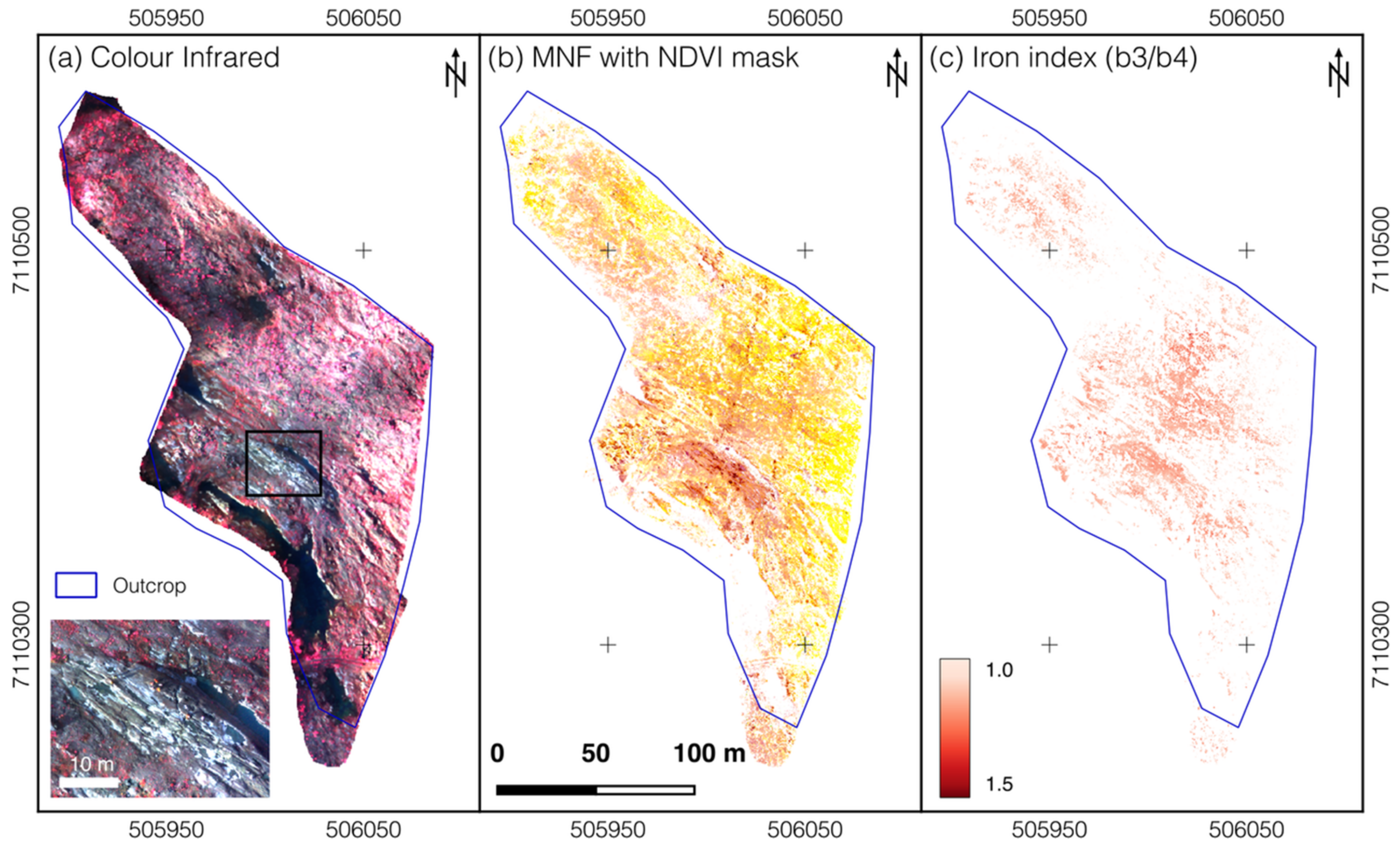
4.1. UAS Multispectral Imagery

The resulting multispectral image mosaic is depicted in Figure 6. While having limited spectral information, the increased spatial coverage is the main advantage of this fixed-wing survey and supplements the multicopter HSI data in areas not captured by HSI.

The Sequoia CIR image (Figure 6a) encompasses the entire outcrop. We identify only little vegetation coverage in the eastern and south-eastern parts of the outcrop. The NDVI mask removes a significant part of pixel in the western region (Figure 6b). The main features in the image are associated with gabbroic rocks and ilmenite-magnetite rock zones in the southern part of the outcrop. Brighter orange-yellow spots (Figure 6b) are related to gabbroic zones and secondary iron minerals. The MNF composite highlights geological characteristics and we can trace structures more easily, for example the shape of outcropping ore bodies. Two parallel trenches, created by surface sampling with a rock saw, are identified in the image centre after MNF transformation.

We calculated an iron band ratio (735/790 nm) for the Sequoia dataset (Figure 6c). The ratio indicates iron related absorption (iron oxides and hydroxides) using the right shoulder of the Fe²⁺/Fe³⁺ charge transfer absorption [46], associated with decreasing reflectance. Similar studies [48] showed that this simple method is suited to evaluate UAS-HSI images. We identify zones of apparent iron absorption, that are layered on top of the rock surfaces.

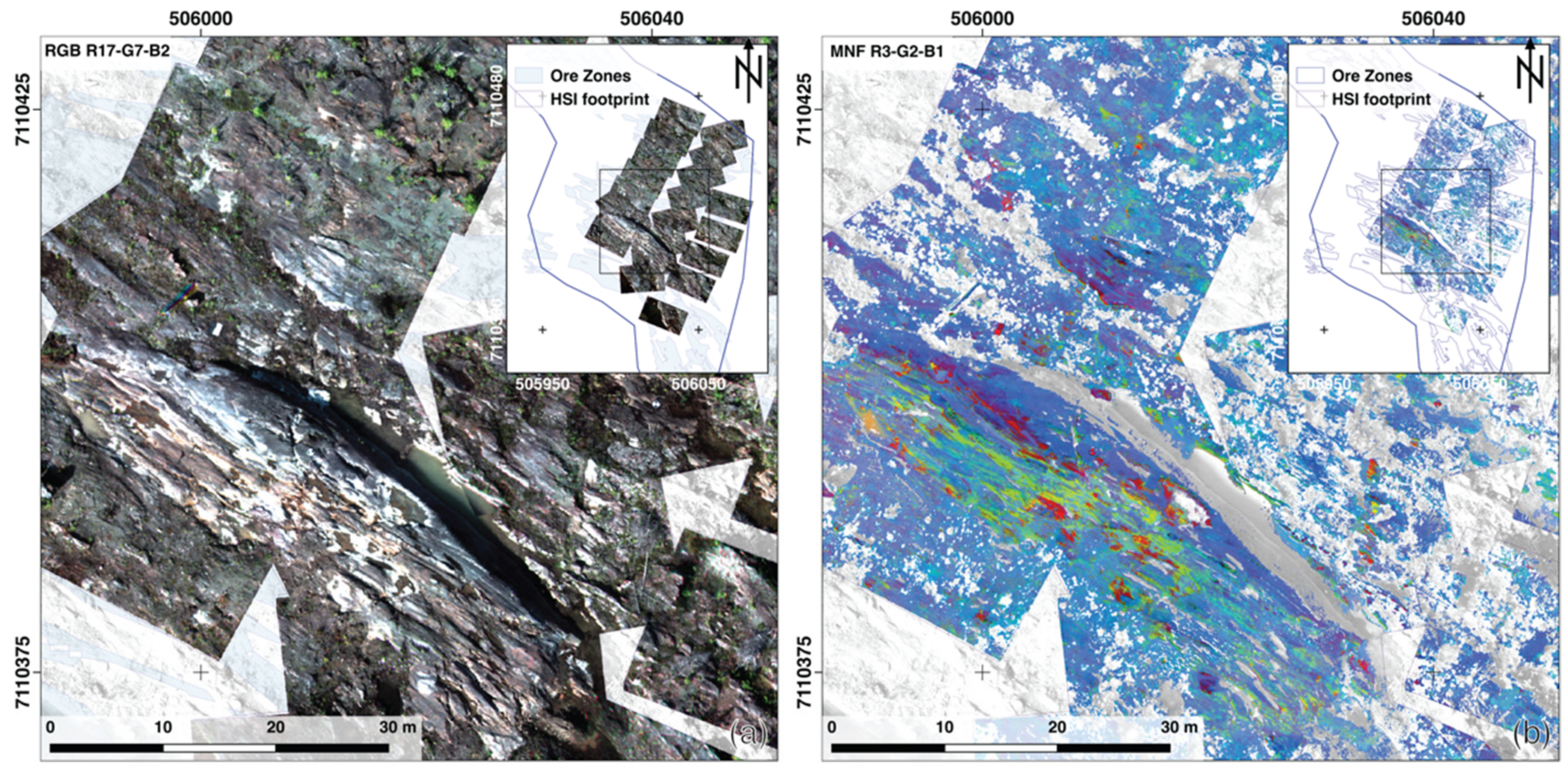
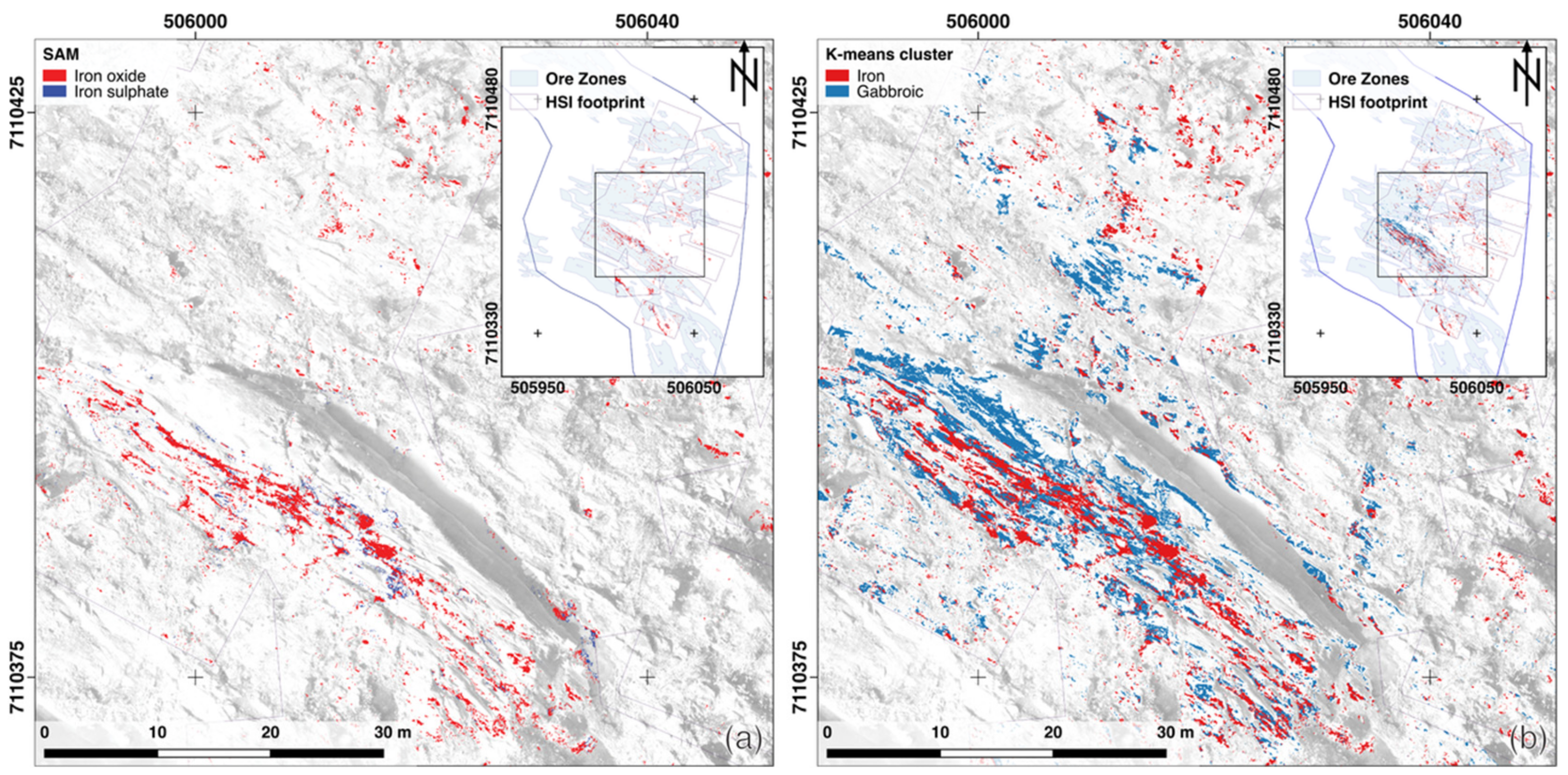
4.2. UAS Hyperspectral Imagery

In total, we covered 17,180 m² of the Metsämalmi outcrop with UAS-HSI data. Parallel ground reconnaissance and the results of multispectral imaging suggested that the eastern part of the outcrop as promising location for remote sensing studies. The other part is densely covered by vegetation (lichen, shrubs, twigs, and young trees). We chose to omit the western area for further interpretation of HSI data. The eastern area is captured by three rows of overlapping HSI scenes (8370 m²) mosaiced into one image (Figure 7). Some hyperspectral scenes have only little or no overlap, as opposed to the used flight plan. We explain this by heading deviations, induced by some distortions of the UAS’s magnetic compass that were caused by the high magnetic anomalies in the area. Roughly 30% of pixels from this mosaic are associated with vegetation and removed with a NDVI mask. The bright patches on the southern ridge are associated with gabbroitic rocks surrounding Fe-Ti-V ore bodies (Figure 7a) which were identified during the ground-based field survey. The sorted MNF false-color image (Figure 7b) shows increased contrast of surface features associated with the different geologic features [59]. We observed increasing vegetation with small patches in the south, growing to a dense cover in the northern area.

The SAM classification in Figure 8a shows the distribution of mapped iron oxides and iron sulphates. We could classify a significant amount of iron oxide and only little iron sulphate, which corresponds to handheld spectroscopy observations. Just two handheld spectra corresponded to iron sulphate. The used iron mineral proxy spectra hematite and goethite are labeled as ‘iron oxide’, and jarosite as ‘iron sulphate’. Two classes from the unsupervised k-means classification (5% change threshold for the cluster centres, 100 iterations) are associated with the in-situ observed features of iron-staining and gabbro. The discarded classes were related to noise, soil-vegetation mixed pixel that remained after NDVI filtering, and potentially redundant features caused by illumination changes. The results for k-means and SAM with respect to the iron minerals are qualitatively comparable, but the SAM classification yields 36.2% less categorized pixels.

We show exemplary spectra acquired from HSI data in Figure 9. They were created by selecting spectra from representative spots in the data (Figure 8a) and combine them in major surface categories (iron oxide, iron sulphate, host rock plus soil, lichen). The selection is based on both observations during the field campaign and inspections of HSI data. We removed five bands in the spectral range of 624–671 nm, where a sensor artefact is noticeable as a flat section. The exemplary spectra related to iron oxide and rock–soil mixture (Figure 9a,c) show small reflectance spread, while the ones associated with iron sulphate and lichen remnants (Figure 9b,d) show larger standard deviations. The average spectral reflectance is low (<30%), which is expected from the study site’s dark surface.

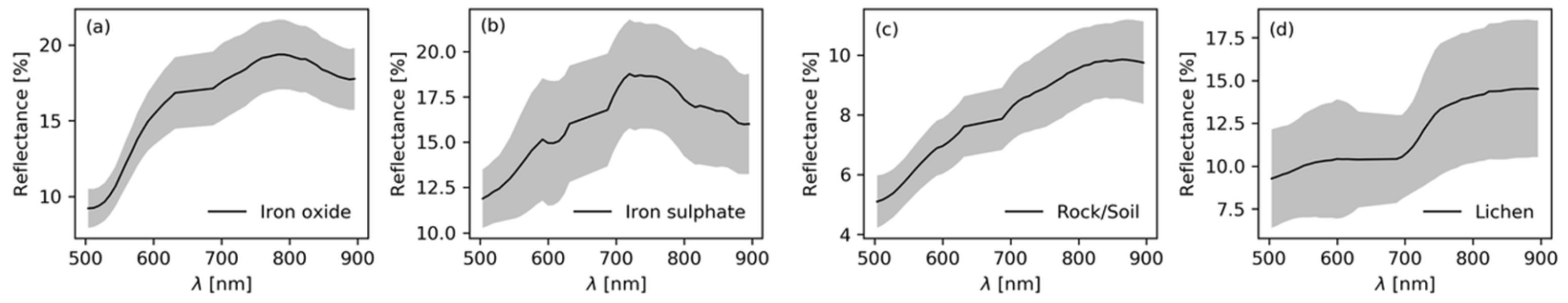
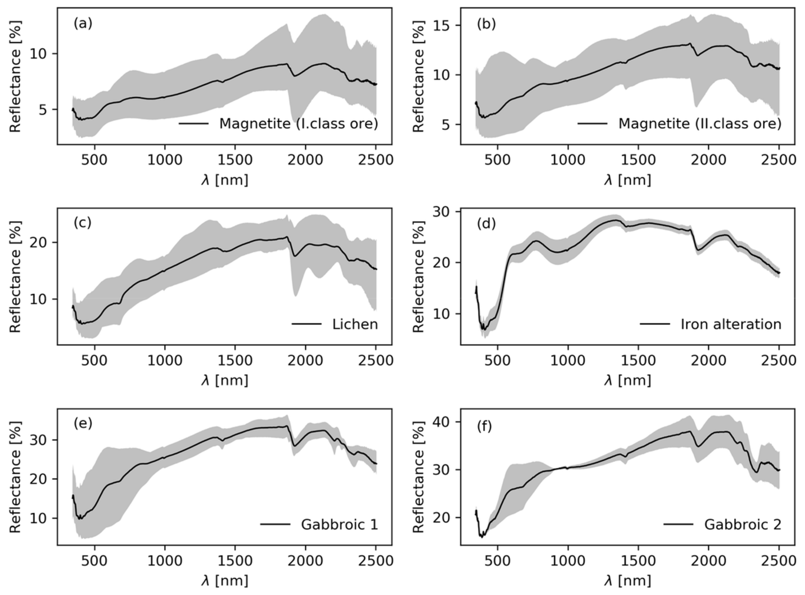
4.3. Handheld Spectroscopy

Figure 10 illustrates the spectral categories that are derived from field spectra acquired along the most western N–S running traverse shown in Figure 2c. The diagnostic absorption features we observe are representative for the mapped geology of Metsämalmi. Distinctive hydroxyl absorption bands around 1400 nm and 1900 nm are visible. The charge transfer with broad absorption between 800–950 nm [46] is dominant for iron-bearing categories (Figure 10a,b,d). In particular, the absorption features for hematite, jarosite, and goethite can be observed in the iron alteration category (Figure 10d), which were attributed to iron sulphate/oxide classes in UAS-borne hyperspectral data. The standard deviation of the iron alteration is small, as seen in Figure 9a and Figure 10d. Amphiboles can be recognized by a specific absorption related to the Mg-OH vibrational overtone at 2310 nm and 2380 nm. The 2200 nm absorption feature was prominent in most spectra and is related to the Al-OH overtone and typical for sheet-silicates and was prominent in most spectra.

The Al-OH feature at 2200 nm, with an accumulation between 2200–2206 nm was mainly found on soil surfaces. The Mg-OH overtone-bending [60] around 2300–2350 nm is related to amphibole-rich rocks (i.e., abundant in amphibolite), and occurs in magnetite-bearing rocks, as well as gabbroic surfaces.

4.4. UAS-HSI Accuracy Assessment

We conducted an accuracy assessment to validate the HSI classifications from SAM and k-means and compared them with the handheld spectra. The 51 handheld scans were scrutinized and labeled according to their major properties: (i) iron oxide-hydroxide (contains magnetite in that category), (ii) iron sulphate, (iii) gabbro; and (iv) lichen. This categorization ensures distinguishable spectra in the spectral range of the Rikola camera. We created a look-up table and attributed the major spectral features between 500–900 nm. Other observed spectral absorption features are related to amphiboles (e.g., hornblende), biotite and clay minerals (e.g., illite, smectite; according to USGS reference spectra). A strong absorption at ~670 nm is diagnostic for chlorophyll and here caused by abundant lichen. From the examined spectra, 21 showed clear iron features with some mixture between hematite, goethite, and jarosite. We labeled the hematite-goethite mixture as iron-oxide and jarosite as iron sulphate, respectively. A map layer with the labeled handheld scans was spatially joint with the SAM result map and classified pixels were counted. We created an eight-pixel buffer around each handheld scan point position to address the measurement deviation. We achieve an overall accuracy of 68.1% for SAM. To validate the k-means approach, 43 spectral points with iron-features or gabbroic characteristics (e.g., amphiboles) were considered within the UAS-HSI mosaic. K-means could not distinguish between two iron features, therefore we grouped iron-oxide and iron sulphates with one label, and use gabbroic as second surface label. The k-means iron class also contains all of the SAM iron oxide pixels. We obtain an overall accuracy of 84.9 % for k-means.

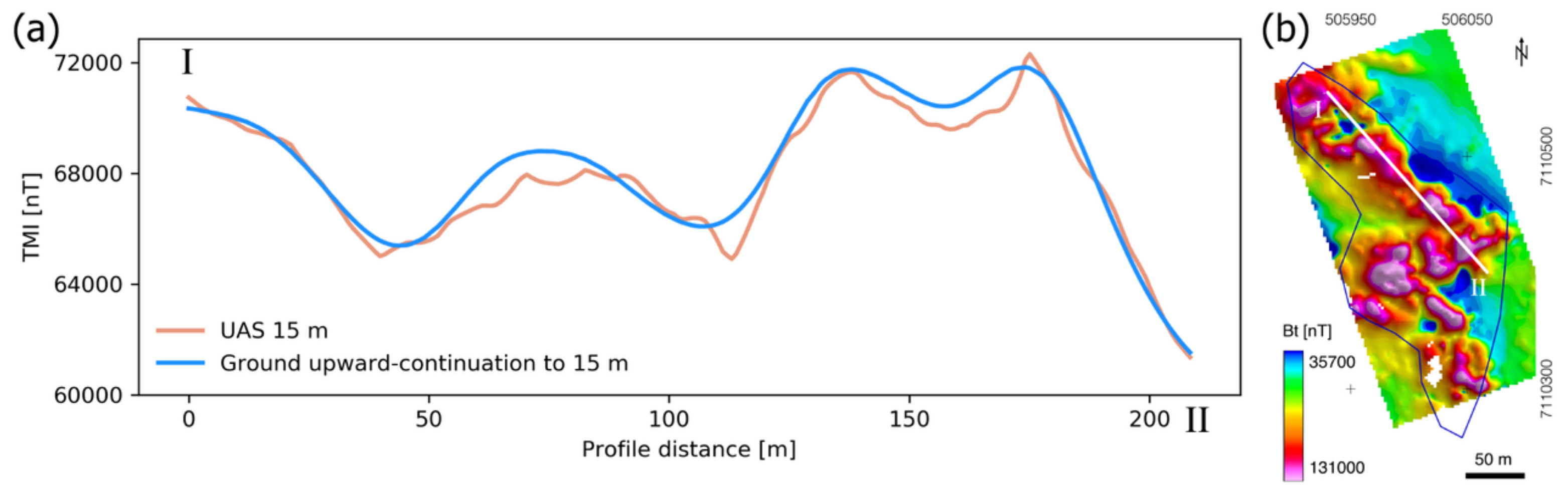
4.5. Magnetics—Ground and UAS-Borne

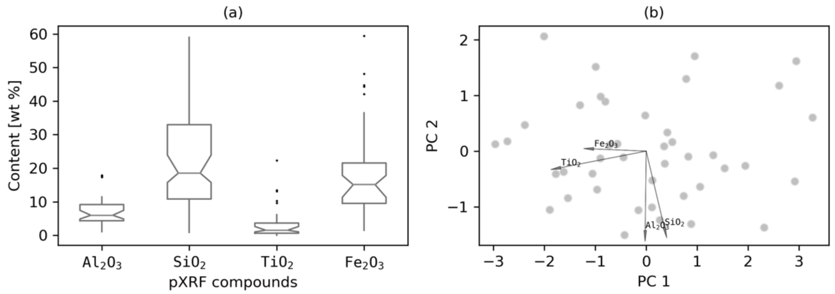
The magnetic measurements with the different UAS platforms, as well as the ground measurements, are presented as TMI in Figure 11. We observe that the TMI anomalies from the magnetic ground survey correlate well with the location of known magnetite-ilmenite ore lenses (Figure 2d). TMI values measured on the ground above known ore zone are high (broadly in a range of 60,000–120,000 nT) indicating the magnetite signature, which is expected, considering that the highest graded ores in Otanmäki contain 35–40% magnetite [61].

The alignment of anomalies from the four UAS surveys with three different heights at 15 m, 40 m, and 65 m are generally in agreement with the overall observed distribution of ore lenses at the surface (compare Figure 11b–e with Figure 2d). The 15 m flight (Figure 11b) captures similar locations of the anomalies lows and highs as seen in the ground data (Figure 11a). However, the actual shape of anomalies from the surveys at 15 m AGL differ already quite a bit from mapped ore lenses at the surface, due to the reduced resolution and the larger impact of deeper ore bodies with larger distance to the surface. With further increasing altitudes of the surveys at 40 and 65 m AGL (Figure 11c–e), the more regional field with broader wavelengths and impact from deeper sources become gradually more dominant. In addition, the coarser line spacing of surveys made at 40 m and 60 m altitude, particularly in the fixed-wing survey, which has the widest line spacing, further lowers the resolution and prohibit resolving the details observed in the ground based and 15 m altitude survey even after filtering is applied.

Statistical details for the magnetic field from the different surveys at the Metsämalmi outcrop area are given for a defined reference area in

Table 6. Comparison of TMI grid values from the same area, shown in Figure 12a.

Parameter (Bt)	Ground Survey	Multicopter 15 m AGL	Multicopter 40 m AGL	Multicopter 65 m AGL	Fixed-Wing 40 m AGL
Min.	37,480 nT	60,130 nT	61,100 nT	60,610 nT	56,400 nT
Max.	131,490 nT	78,980 nT	67,370 nT	64,790 nT	61,240 nT
Mean	68,140 nT	69,960 nT	64,250 nT	63,170 nT	59,320 nT

(see this area outlined with a rectangle in Figure 11a).

Note that in Figure 11e, only a small part of the resulting 40 m fixed-wing survey is presented and that the complete survey of ~1 × 1 km covers large parts of the eastern part of the Otanmäki ore deposit and the adjacent rock units (results from areas apart from the outcrop are not presented here). For all surveys, we observe a high magnetic anomaly in the central part of Metsämalmi (Figure 11). Particularly for the fixed-wing survey, it is observed that magnetic values follow a general lateral trend, having a negative gradient towards the north-eastern border of the marked outcrop area. We also noticed that the highest magnetic anomalies were located at the same positions for all five surveys.

Figure 12 compares two profiles of TMI values from the 15 m UAS and ground magnetic survey, whose data are upward-continued to 15 m. The magnetic profiles have a good overall resemblance in shape and intensity and suggest a high correlation of both datasets.

4.6. Geochemistry

The four main elemental constituents (Figure 13a) of Metsämalmi are measured by pXRF (n = 72, values in average (avg.) wt % (weight %) in their oxide forms (see Figure 13a). Bulk constituents are silica (21.9 wt % avg. SiO₂), followed by iron (17.9 wt % avg. Fe₂O₃), aluminium (6.9 wt % avg. Al₂O₃) and titan (3.2 wt % avg. TiO₂). The silica content shows the widest range, while iron concentrations have the most outliers. Sulphur and vanadium oxide content amount to ~1.0 wt % and 0.1 wt %, respectively. Therefore, those two lie outside of the pXRF calibration and are not plotted here.

We applied principal component analysis of the elemental compositions to visualize the relationship between the element variables [62]. The values for V and S were excluded from the PCA, due to strong outliers. The pXRF data was converted into log-ratios by the log-ratio transformation [63,64] for scale invariance and to avoid spurious correlations [65], and the PCA was applied on the transformed values (first two PC’s explain 92% of the variance).

The log-ratios Si/Al and Fe/Ti are approximately constant, since the variable rays are close (Figure 13b). The log-ratios between Fe and Ti versus Si and Al do not correlate, which is seen as the orthogonal vector pairs. Hence, Ti occurrence correlates with iron abundance, and therefore in the present case we can use iron occurrence as proxy for ilmenite presence.

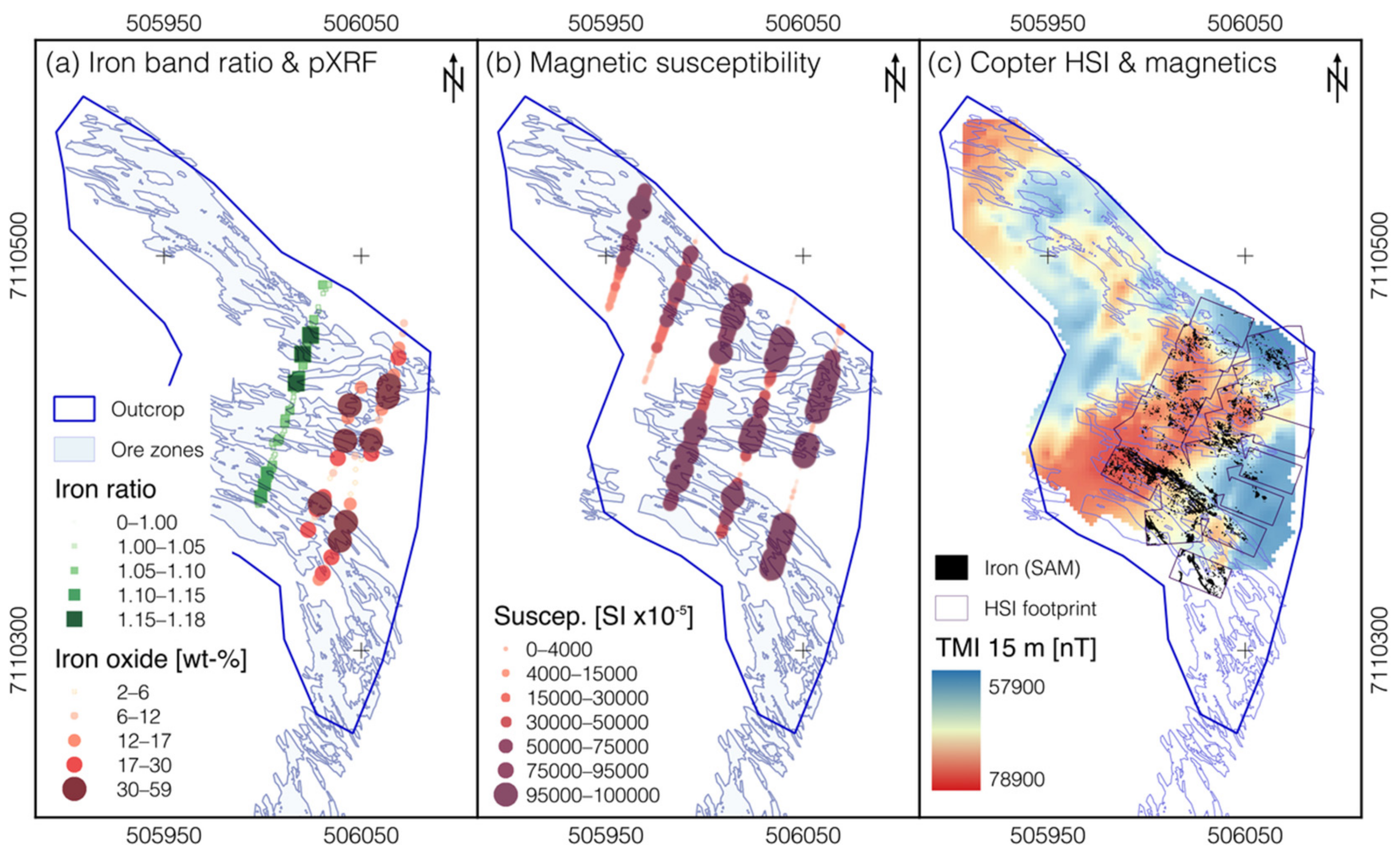
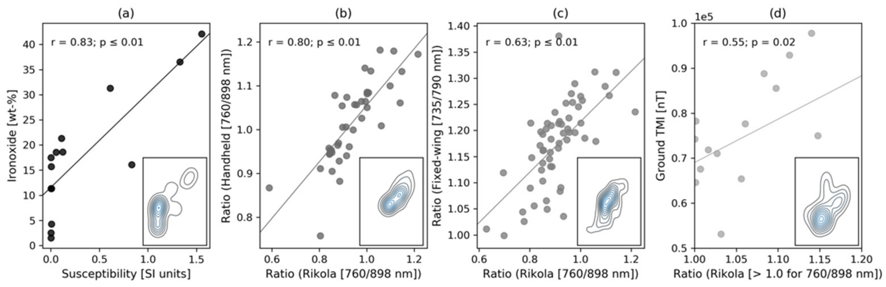
4.7. Integration of Ground Truth and Multicopter Data

The pXRF iron readings and computed iron ratios from handheld spectroscopy are mapped in Figure 14a. The depicted values spatially correlate with the mapped ore zones. Figure 14b displays five selected surface profiles of susceptibility measurements (n = 4,524) ranging between 0–1 SI units. With point distances between 2–3 cm per scan, those spots enable the tracing of main ore zones. We regard those measurements as quantitative evidence of high susceptibility of the top surface material and discard remnant magnetization.

The multicopter TMI data from the 15 m AGL flight is plotted in Figure 14c, together with the HSI footprint and the result of the SAM iron classification. Generally, we observe increased surface iron occurrence aloft high TMI values. Iron absorption is also observed, right above the water table of small water bodies due to weathering, and along the HSI mosaic’s NS axis. The prominent lateral ridge in the south of the HSI features most iron-indicating pixels, while also showing the highest TMI values in all magnetic plots (Figure 11a). The corresponding measurements of ground validation are presented in Section 4.8.

4.8. Data Integration

Surface observations with different techniques allow a characterization of the general area and reflect the originally mapped local geology and mineralogy (i.e., magnetite, ilmenite, amphiboles, gabbro).

We compare the different GNSS-measured ground validation and UAS-borne datasets (Figure 15). The extracted measurements were taken on the same spot as the corresponding pixel of UAS data. The correlation coefficients (Pearson’s correlation r) show an overall agreement. The high correlation (r = 0.83) for pXRF vs. susceptibility (Figure 15a) compares ore bodies with best ore grades, that should contain high iron content. The highest observed pXRF iron oxide content (41.5 wt % Fe) was described optically as ‘pure magnetite’ in the field. The UAS-HSI band ratio is probed with the known validation points, and compared with the iron ratios (r = 0.80) of the handheld spectrometer (Figure 15b). Likewise, values from both UAS camera sample spots are plotted (Figure 15c), to compare the Sequoia with the Rikola performance (r = 0.63).

An illustration of extracted ground magnetic measurements compared with iron absorption depths depicts an association (r = 0.55) with the trend visible in Figure 15d. The correlations demonstrate, that the datasets from multiple sources can be jointly interpreted.

4.9. Geologic Interpretation and Ore Class Estimation

With a joint interpretation of all acquired UAS-borne datasets, we can give a semi-automatic structural interpretation and ore occurrence estimation [66]. Structural features (lineaments and discontinuities) show us the directional trend in the outcrop. The extraction (Figure 16a) was done automatically and help to map the structural NW–SE trend. However, as vegetation and debris cover could not completely be removed from the DEM, the extracted lineaments were manually refined afterwards.

For the purpose of data integration, we first resampled different grid resolutions to one. We choose the 15 m UAS-TMI as a representative footprint. In order to rescale and match data to the UAS-TMI grid, the HSI and MSI data were resampled to 2 m grid size, using the mean cell values (Figure 16b). We estimated an ore prospectivity in the following:

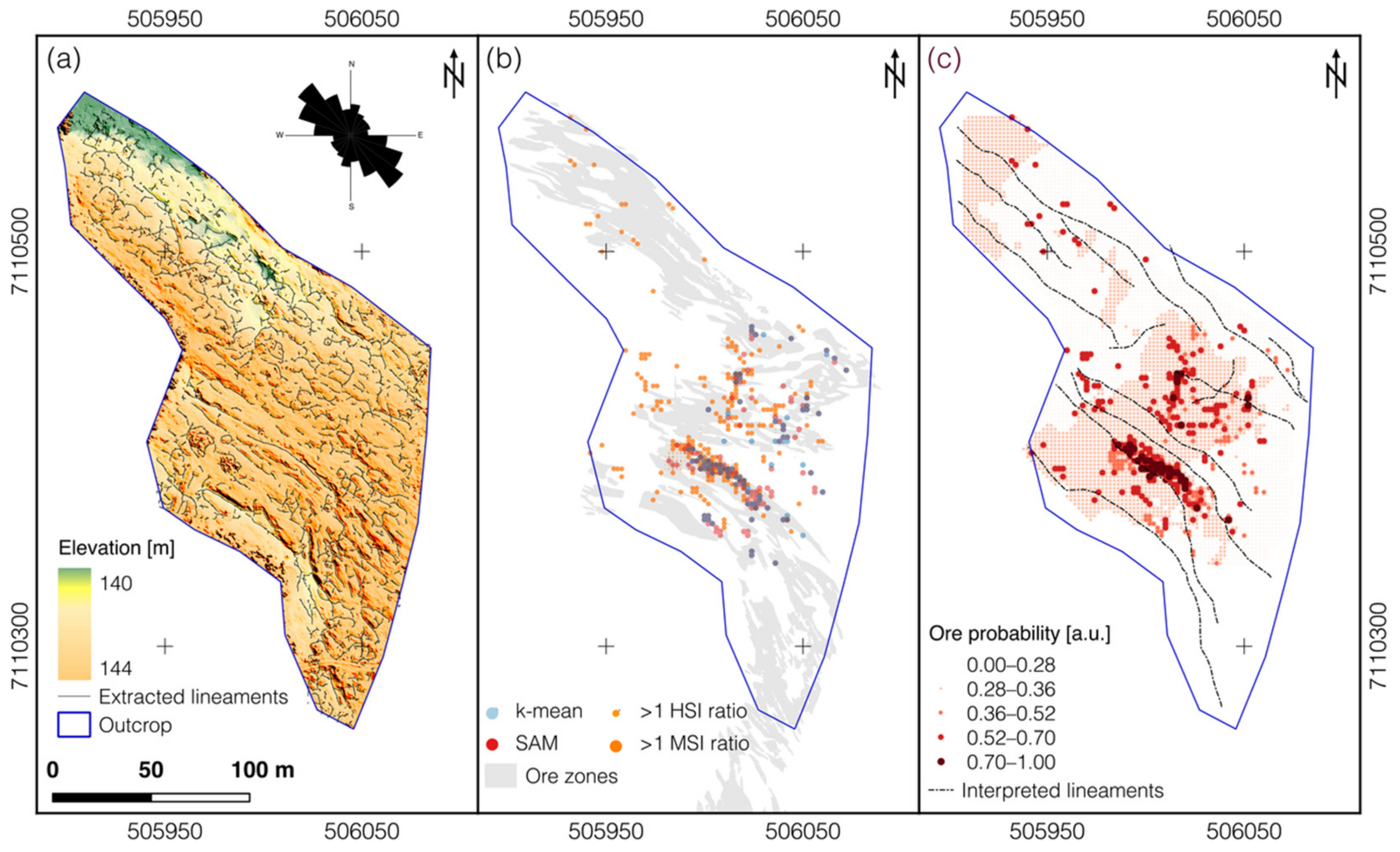
• MSI and HSI UAS surface classifications were binarized (unclassified and classified pixels are either 0 or 1) and the 15 m TMI data was normalized between 0–1. By doing so, mostly the highest TMI areas contribute to the surface feature map.
• Normalized weighted arithmetic mean of the HSI, MSI and TMI datasets was computed.
• High values in the resulting map (Figure 16c) represent high ore probability.
• Interpreted lineaments are spatially joined with the proceptivity map, to give structural context.

Finally, Figure 16c allows an estimation of ore occurrence along the surface. We observe a relationship between iron-indication surface pixel and sub-surface magnetic features, that follow the directional trend of the local morphology. The directional trend of the iron ore from NW to SE is illustrated.

5. Discussion

5.1. Consequences of UAS Imaging

The results of multispectral survey require careful examination. With the Sequoia camera, the bandwidths of band 3 (10 nm) vs. band 4 (40 nm) differ, therefore band 4 covers important spectral characteristics of iron-bearing minerals (e.g., hematite, goethite, jarosite, and copiapite). Still, the comparison of HSI vs. MSI indicates a correlation (Figure 16c). The MSI data seems to overestimate iron-abundance and reasons are likely differing sampling distances, randomly distributed lichen coverage, and mainly the challenge to spectrally detect magnetite. The two excavated sampling ridges along the outcrop feature iron stains, which indicates displaced weathered surface or even fresh rock.

The spectral artefact of the HSI camera between ~636–650 nm, is caused by its two-sensor design [67] and was removed. We recommend an HSI camera setting of 50 bands with 8 nm spectral resolution as most effective to maintain a balance between spectral density and SNR.

Noise reduction by PCA techniques (i.e., MNF) increases the reliability of our unsupervised classifications. We observe that in MNF-transformed hypercubes, features (e.g., surface patterns related to geology and morphology) remain even in high-order, low-variance MNF dimensions. Unsupervised separation of surface classes (i.e., k-means) is based on spectrally contrasting mineral groups. In the presented case, the surface distinctions account predominantly for iron-rich and iron-poor rock surfaces. Further examination and correlation of classification results with field observations and orthophotography imply that the achieved separations are associated with iron-bearing and gabbroic areas. We found that iron-sulphates are not resolved by k-means and are partially mixed in the resulting iron class.

The SAM classification achieved a separation of iron-oxides-hydroxides and iron-sulphates with reduced classified pixels. This reduction can be caused by illumination changes or strongly mixed surface materials.

The Metsämalmi outcrop has been exposed for several decades, that leads to significant cover of surface portions by lichen, shrubs and small trees, that we observed in-situ. Thus, important features were hidden to the UAS cameras, which affects for example the correlation of ground TMI and UAS-HSI (Figure 15d). The mentioned surface cleaning is possibly uneconomic, but we had no direct influence on the procedure. Advantage of the frame-based HSI camera is the capability to create spatially undistorted images, even under wrong flight headings of the UAS, caused by magnetic interference.

5.2. Consequences of UAS Magnetic Measurements

We compare the UAS survey with ground data for a benchmark. The ground survey took two full days in the field to cover 50,500 m². A similar area was covered using two UAS flights in ~45 minutes. Data processing time is not considered, since we developed the processing routines during this study and those can be applied quickly.

The sensors z-component saturation in 1% of the magnetic raw data was caused by the combination of an extremely strong anomaly, shallow flight height and the magnetometer’s measurement range. This can be avoided by using a similarly constructed fluxgate magnetometer with a larger dynamic range or a slight increase of the survey altitude. Also, the strong regional magnetic field influences every measurement and makes a comparison (for example Figure 15d) challenging. The navigation and recovery of the UAS’s absolute position is also influenced by the anomaly and caused a slight shift between two fused survey flights (Figure 11b). Structural field measurements with a geologic compass were strongly affected by the local magnetic field, which made field observations challenging.

Flight line geometry is a fundamental aspect of magnetic survey; hence, we observe differences between the 40 m copter and 40 m fixed-wing data. The applied cell size in the minimum curvature interpolation also contributes to mapping differences. Figure 11c,e show varying TMI ranges, and the values of Table 6 indicate contrasting centers. One major reason for the differences in the data of both altitudes are orientation and density of the flight pattern. The 40 m multicopter flight had denser lines, was flown perpendicular to the strike of ore bodies, and captured higher anomaly amplitudes at different locations. Furthermore, the workflows of multicopter and fixed-wing data surveys are slightly different. The fixed-wing acquisition uses a combination of ancillary sensor input and inversion modeling, while the multicopter uses calibration flights and benefits from its capability of getting closer to the surface. The used ELM for the fixed-wing survey reduces effects of varying flight altitude and uneven data point sampling. It also removes high frequency noise and artefacts (e.g., from electric power lines and UAS engine noise) provided that their wavelength is short compared to the size of the elements used in the computed layer model. Yet, the results of both UAS survey methods allow the visualization of the anomaly patterns. We note that the relative altitude measurements per UAS flight slightly deviate per line. We observed an upward drift (~1 m/10 min) in the barometer records for the 65 m, which could be caused by an atmospheric pressure change. It is assumed that all our multicopter measurements endure an altitude deviation of at least ± 1 m from the unknown true values, based of GPS and barometer data evaluation.

Non-linear sensor noise and the creation of aliasing effects takes place which induces a binning effect on the sampling process. Studies suggested methods to address UAS noise, for example an increase of the sensor distance to noise sources and an adapted compensation in real-time or in post-processing [68,69].

5.3. Can Drone-Borne Analysis Compete with Airborne Survey and Outperform Ground-Based Acquisition?

For optical remote sensing, the Sequoia camera data shows the possibilities (large area) and limitations (insufficient bands) of a multispectral UAS camera for mineral exploration. We note the correlation (r = 0.63) between a working concept (i.e., UAS-HSI) and this experiment (UAS-MSI).

The lichen-debris cover reduced the total amount of visible rock-containing pixels by roughly 30%. Image classifications of remaining areas reveal iron-bearing alteration minerals, that we used as proxies for the target mineral magnetite. Ground spectroscopy validated the hyperspectral results (r = 0.80), however the chosen study area had harsh conditions for this hypothesis.

The overall accuracy of SAM for two iron minerals is reported with 68%, while the unsupervised k-means classification for iron oxide and host rock is 84%. We used various instruments to validate the UAS-borne datasets in situ. The results of pXRF scans during our fieldwork correspond with results reported by the mining company.

We observe a correlation (r = 0.55) between UAS-HSI iron ratio vs. ground truth TMI. Again, the strong regional anomaly skews those observations. To avoid spurious correlation, we examined outliers and none are removed from the data-set. In that regard, we stress out the fundamental difference, as the TMI signal is the superposition from any subsurface anomaly of differing depth, while the UAS-HSI data arises from the surface alone.

In terms of image resolution, the UAS imagery performs satisfying and creates pixel sizes of 2.2 cm (orthophoto), 3.0 cm (HSI), and 7.4 cm (MSI), while the mean point distance between handheld spectral measurements is 2 m. Those data are orthorectified by accurate GCPs. Similarly, the 15 m UAS magnetics feature a line spacing of 7 m, while the ground survey achieved 10 m. Evidently, using UAS reduces time and effort to achieve quality results for a reasonable aerial coverage. We observe that the time needed, as seen in Table 5, outperforms ground-based survey. With our current setup and an estimation based on the survey times and line spacing, we achieved 7.6–8.9 line km per hour (UAS in-air time). Still, ground sampling is required, and survey time constraints could be mitigated in countries with abundant low-cost workforce. The data processing, while under constant development, can be done in hours, results in meaningful maps during a field campaign, and creates streamlined and efficient workflows.

The tested sensors require some calibration effort, and the UAS provides flexibility by a quick-release connector used to rapidly switch from magnetic to hyperspectral instruments. A further UAS advantage is the possibility to carry out the surveys by one trained person, that can fly different UAS types over any kind of terrain. We note that the characteristics of the survey area need to be specified, e.g., to avoid such deviations from the flight patterns caused by the high TMI.

We see several outcomes of integrating various UAS datasets:

• Consistency of models is maintained (e.g., high spatial precision).
• Improved reliability and reduced errors in mapping and predictions.
• Classification of domains (e.g., minerals, surface and subsurface structures) that consist of several non-linear features.
• The applicability of multi-spectral UAS data for derivation of traces, structures, and shapes of geological features.

6. Conclusions

Within two-and-a-half days of fieldwork, a detailed mapping of the Metsämalmi outcrop in the Otanmäki mining district was achieved. The dataset includes surficial morphology, mineral distributions and the shape of the local magnetic anomaly at five scales. We used hyperspectral image mosaics with band ratios and classification algorithms to delineate iron-bearing mineral phases on the surface. We covered three magnetic flight altitudes (15 m, 40 m, and 65 m AGL) on an outcrop scale with a multicopter, and performed a regional scale survey (40 m AGL with 69 km of survey lines) using a fixed-wing UAS. The magnetic data acquisitions were performed fast, and flight planning for the magnetic surveys was optimized to cover as much of the outcrop as possible, while staying under the maximum battery endurance of the UAS.

Data integration of dense magnetic susceptibility profiling correlates well with magnetic field mapping and ore occurrences. The high-resolution surface imagery and subsurface information of the magnetic field are fused and jointly interpreted. Their combined plot leads to a semi-automatically created geologic map that distributes iron occurrences which directly relate to the ore.

Based on the multiple datasets for the Metsämalmi area, we draw the following conclusions:

• Iron-bearing phases can be successfully mapped by both UAS-borne multi- and hyperspectral sensors in the VNIR.
• UAS-borne fluxgate magnetometers are able to map magnetic anomalies under survey conditions.
• Low altitude (i.e., 15 m AGL) multicopter magnetic data correlates to ground survey magnetic data, while higher flight altitude data describes the regional magnetic field.
• Magnetic anomalies can be associated to spectral anomalies at the surface by using ground truth.
• UAS-HSI and magnetic survey complement each other.

The combination of light-weight UAS technology with RGB, multi- and hyperspectral cameras and fluxgate magnetometers is advantageous and created a basis for integrated data analysis. We demonstrate that the UAS approach for non-invasive mineral exploration based on integration of remote sensing and geophysical techniques is successful, based on comparable UAS and ground survey results. The joint UAS datasets for the prospectivity map display how extracted lineaments, spectra, and magnetics form a base map for visual interpretation. Our findings highlight the advantages of UAS as a practical, fast, and comfortably deployable geoscientific tool, that creates high resolution data within short turn-around times.

In summary, we conclude that UAS-borne surveys can compete with ground surveying, while having a reduced cost overhead. We assume that integrated UAS surveys in mineral exploration and mining will reduce the amount needed of exploration drillings in future. Time for ground personnel to be exposed in dangerous areas will be limited and the repeated acquisitions can be used for further examination of targets and environments, during the entire mine-life cycle. The presented survey approach should be further tested on more and different types of geologic targets in the future.

References

1. Schoer, K.; Weinzettel, J.; Kovanda, J.; Giegrich, J.; Lauwigi, C. Raw Material Consumption of the European Union–Concept, Calculation Method, and Results. Environ. Sci. Technol. 2012, 46, 8903–8909. [Google Scholar] [CrossRef]
2. Massari, S.; Ruberti, M. Rare earth elements as critical raw materials: Focus on international markets and future strategies. Resour. Policy 2013, 38, 36–43. [Google Scholar] [CrossRef]
3. Ali, S.H.; Giurco, D.; Arndt, N.; Nickless, E.; Brown, G.; Demetriades, A.; Durrheim, R.; Enriquez, M.A.; Kinnaird, J.; Littleboy, A.; et al. Mineral supply for sustainable development requires resource governance. Nature 2017, 543, 367–372. [Google Scholar] [CrossRef]
4. The European Commission. Communication from the Commission to the European Parliament, the Council, The European Economic and Social Committee and the Committee of the Regions on the 2017 List of Critical Raw Materials for the EU; EU: Brussels, Belgium, 13 September 2017. [Google Scholar]
5. Gloaguen, R.; Ghamisi, P.; Lorenz, S.; Kirsch, M.; Zimmermann, R.; Booysen, R.; Andreani, L.; Jackisch, R.; Hermann, E.; Tusa, L.; et al. The Need for Multi-Source, Multi-Scale Hyperspectral Imaging to Boost Non-Invasive Mineral Exploration. In Proceedings of the IGARSS 2018-2018 IEEE International Geoscience and Remote Sensing Symposium, Valencia, Spain, 22–27 July 2018; pp. 7430–7433. [Google Scholar]
6. Henckens, M.L.C.M.; van Ierland, E.C.; Driessen, P.P.J.; Worrell, E. Mineral resources: Geological scarcity, market price trends, and future generations. Resour. Policy 2016, 49, 102–111. [Google Scholar] [CrossRef] [Green Version]
7. Stöcker, C.; Bennett, R.; Nex, F.; Gerke, M.; Zevenbergen, J. Review of the current state of UAV regulations. Remote Sens. 2017, 9, 459. [Google Scholar] [CrossRef]
8. Parshin, A.V.; Morozov, V.A.; Blinov, A.V.; Kosterev, A.N.; Budyak, A.E. Low-altitude geophysical magnetic prospecting based on multirotor UAV as a promising replacement for traditional ground survey Low-altitude geophysical magnetic prospecting based on multirotor UAV as a promising replacement for traditional ground survey. Geo-Spat. Inf. Sci. 2018, 1–8. [Google Scholar] [CrossRef]
9. Colomina, I.; Molina, P. Unmanned aerial systems for photogrammetry and remote sensing: A review. ISPRS J. Photogramm. Remote Sens. 2014, 92, 79–97. [Google Scholar] [CrossRef] [Green Version]
10. Rauhala, A.; Tuomela, A.; Davids, C.; Rossi, P.M. UAV remote sensing surveillance of a mine tailings impoundment in Sub-Arctic conditions. Remote Sens. 2017, 9, 1318. [Google Scholar] [CrossRef]
11. Salvini, R.; Mastrorocco, G.; Seddaiu, M.; Rossi, D.; Vanneschi, C. The use of an unmanned aerial vehicle for fracture mapping within a marble quarry (Carrara, Italy): Photogrammetry and discrete fracture network modeling. Geomat. Nat. Hazards Risk 2017, 8, 34–52. [Google Scholar] [CrossRef]
12. Zarco-Tejada, P.J.; Guillén-Climent, M.L.; Hernández-Clemente, R.; Catalina, A.; González, M.R.; Martín, P. Estimating leaf carotenoid content in vineyards using high resolution hyperspectral imagery acquired from an unmanned aerial vehicle (UAV). Agric. For. Meteorol. 2013, 171–172, 281–294. [Google Scholar] [CrossRef]
13. Ham, Y.; Han, K.K.; Lin, J.J.; Golparvar-Fard, M. Visual monitoring of civil infrastructure systems via camera-equipped Unmanned Aerial Vehicles (UAVs): A review of related works. Vis. Eng. 2016, 4, 1. [Google Scholar] [CrossRef]
14. Koucká, L.; Kopačková, V.; Fárová, K.; Gojda, M. UAV Mapping of an Archaeological Site Using RGB and NIR High-Resolution Data. Proceedings 2018, 2, 351. [Google Scholar] [CrossRef]
15. Näsi, R.; Honkavaara, E.; Lyytikäinen-Saarenmaa, P.; Blomqvist, M.; Litkey, P.; Hakala, T.; Viljanen, N.; Kantola, T.; Tanhuanpää, T.; Holopainen, M. Using UAV-Based Photogrammetry and Hyperspectral Imaging for Mapping Bark Beetle Damage at Tree-Level. Remote Sens. 2015, 7, 15467–15493. [Google Scholar] [CrossRef] [Green Version]
16. Restas, A. Drone applications for supporting disaster management. World J. Eng. Technol. 2015, 3, 316. [Google Scholar] [CrossRef]
17. Mancini, F.; Dubbini, M.; Gattelli, M.; Stecchi, F.; Fabbri, S.; Gabbianelli, G. Using Unmanned Aerial Vehicles (UAV) for High-Resolution Reconstruction of Topography: The Structure from Motion Approach on Coastal Environments. Remote Sens. 2013, 5, 6880–6898. [Google Scholar] [CrossRef] [Green Version]
18. Rahman, M.M.; McDermid, G.J.; Strack, M.; Lovitt, J. A New Method to Map Groundwater Table in Peatlands Using Unmanned Aerial Vehicles. Remote Sens. 2017, 9, 1057. [Google Scholar] [CrossRef]
19. Bemis, S.P.; Micklethwaite, S.; Turner, D.; James, M.R.; Akciz, S.; Thiele, S.T.; Bangash, H.A. Ground-based and UAV-Based photogrammetry: A multi-scale, high-resolution mapping tool for structural geology and paleoseismology. J. Struct. Geol. 2014, 69, 163–178. [Google Scholar] [CrossRef]
20. James, M.R.; Robson, S. Mitigating systematic error in topographic models derived from UAV and ground-based image networks. Earth Surf. Process. Landf. 2014, 39, 1413–1420. [Google Scholar] [CrossRef] [Green Version]
21. Malehmir, A.; Dynesius, L.; Paulusson, K.; Paulusson, A.; Johansson, H.; Bastani, M.; Wedmark, M.; Marsden, P. The potential of rotary-wing UAV-based magnetic surveys for mineral exploration: A case study from central Sweden. Lead. Edge 2017, 36, 552–557. [Google Scholar] [CrossRef]
22. Kirsch, M.; Lorenz, S.; Zimmermann, R.; Tusa, L.; Möckel, R.; Hödl, P.; Booysen, R.; Khodadadzadeh, M.; Gloaguen, R. Integration of Terrestrial and Drone-Borne Hyperspectral and Photogrammetric Sensing Methods for Exploration Mapping and Mining Monitoring. Remote Sens. 2018, 10, 1366. [Google Scholar] [CrossRef]
23. Dering, G.M.; Micklethwaite, S.; Thiele, S.T.; Vollgger, S.A.; Cruden, A.R. Review of drones, photogrammetry and emerging sensor technology for the study of dykes: Best practises and future potential. J. Volcanol. Geotherm. Res. 2019. [Google Scholar] [CrossRef]
24. Gavazzi, B.; Le Maire, P.; Munschy, M.; Dechamp, A. Fluxgate vector magnetometers: A multisensor device for ground, UAV, and airborne magnetic surveys. Lead. Edge 2016, 35, 795–797. [Google Scholar] [CrossRef] [Green Version]
25. Tezkan, B.; Stoll, J.B.; Bergers, R.; Großbach, H. Unmanned aircraft system proves itself as a geophysical measuring platform for aeromagnetic surveys. First Break 2011, 29, 103–105. [Google Scholar]
26. Koyama, T.; Kaneko, T.; Ohminato, T.; Yanagisawa, T.; Watanabe, A.; Takeo, M. An aeromagnetic survey of Shinmoe-dake volcano, Kirishima, Japan, after the 2011 eruption using an unmanned autonomous helicopter. Earth Planets Sp. 2013, 65, 657–666. [Google Scholar] [CrossRef] [Green Version]
27. Cunningham, M.; Samson, C.; Wood, A.; Cook, I. Aeromagnetic Surveying with a Rotary-Wing Unmanned Aircraft System: A Case Study from a Zinc Deposit in Nash Creek, New Brunswick, Canada. Pure Appl. Geophys. 2018, 175, 3145–3158. [Google Scholar] [CrossRef]
28. Parvar, K.; Braun, A.; Layton-Matthews, D.; Burns, M. UAV magnetometry for chromite exploration in the Samail ophiolite sequence, Oman. J. Unmanned Veh. Syst. 2018, 6, 57–69. [Google Scholar] [CrossRef]
29. Callum, W.; Braun, A.; Fotopoulos, G. Impact of 3-D attitude variations of a UAV magnetometry system on magnetic data quality. Geophys. Prospect. 2018, 1–15. [Google Scholar]
30. Samson, C.; Straznicky, P.; Laliberté, J.; Caron, R.; Ferguson, S.; Archer, R. Designing and Building an Unmanned Aircraft System for Aeromagnetic Surveying. In SEG Technical Program Expanded Abstracts; Society of Exploration Geophysicists: Tulsa, OK, USA, 2010; pp. 1167–1171. [Google Scholar] [CrossRef]
31. Airo, M.-L. Aerogeophysics in Finland 1972–2004: Methods, System Characteristics and Applications. In Special Paper-Geological Survey of Finland; Society of Exploration Geophysicists: Tulsa, OK, USA, 2005; Volume 39, 197p. [Google Scholar]
32. Pääkkönen, V. Otanmäki—The Ilmenite Magnetite Ore Field in Finland. In Bull. la Commision Geol. Finlande; Geological Survey of Finland: Espoo, Finland, 1956; p. 87. [Google Scholar]
33. Lindholm, O.; Anttonen, R. Geology of the Otanmäki mine. In Proc. 26th Int. Geol. Congr. Guid. to Excursions 078 A+C, Part 2 (Finland); Häkli, T.A., Ed.; Mindat: Keswick, VA, USA, 1980; pp. 25–33. [Google Scholar]
34. Huhma, H.; Hanski, E.; Kontinen, A.; Vuollo, J.; Mänttäri, I.; Lahyey, J. Sm–Nd and U–Pb isotope geochemistry of the Palaeoproterozoic mafic magmatism in eastern and northern Finland. Bulletin 2018, 405, 150. [Google Scholar]
35. Lahti, I.; Salmirinne, H.; Kärenlampi, K.; Jylänki, J. Geophysical surveys and modeling of Nb–Zr–REE deposits and Fe–Ti–V ore-bearing gabbros in the Otanmäki area, central Finland. In GTK Open File Work Report; Geological Survey of Finland: Espoo, Finland, 2018; Volume 75, pp. 1–31. [Google Scholar]
36. Hokka, J.; Lepistö, S. JORC Report-Mineral Resource Estimate for Otanmäki V-Ti-Fe Project; Geological Survey of Finland: Espoo, Finland, 2018. [Google Scholar]
37. James, M.R.; Robson, S.; d’Oleire-Oltmanns, S.; Niethammer, U. Optimising UAV topographic surveys processed with structure-from-motion: Ground control quality, quantity and bundle adjustment. Geomorphology 2017, 280, 51–66. [Google Scholar] [CrossRef] [Green Version]
38. Jakob, S.; Zimmermann, R.; Gloaguen, R. The Need for Accurate Geometric and Radiometric Corrections of Drone-Borne Hyperspectral Data for Mineral Exploration: MEPHySTo-A Toolbox for Pre-Processing Drone-Borne Hyperspectral Data. Remote Sens. 2017, 9, 88. [Google Scholar] [CrossRef]
39. Makelainen, A.; Saari, H.; Hippi, I.; Sarkeala, J.; Soukkamaki, J. 2D Hyperspectral Frame Imager Camera Data in Photogrammetric Mosaicking. Int. Arch. Photogramm. Remote Sens. Spat. Inf. Sci. 2013, 1, 263–267. [Google Scholar] [CrossRef]
40. Karpouzli, E.; Malthus, T. The empirical line method for the atmospheric correction of IKONOS imagery. Int. J. Remote Sens. 2003, 24, 1143–1150. [Google Scholar] [CrossRef]
41. Tucker, C.J. Red and photographic infrared linear combinations for monitoring vegetation. Remote Sens. Environ. 1979, 8, 127–150. [Google Scholar] [CrossRef] [Green Version]
42. Green, A.A.; Berman, M.; Switzer, P.; Craig, M.D. A Transformation for Ordering Multispectral Data in Terms of Image Quality with Implications for Noise Removal. IEEE Trans. Geosci. Remote Sens. 1988, 26, 65–74. [Google Scholar] [CrossRef]
43. Tou, J.T.; Gonzalez, R.C. Pattern Recognition Principles; Addison-Wesley Pub. Co.: Boston, MA, USA, 1974. [Google Scholar]
44. Kruse, F.A.; Lefkoff, A.B.; Boardman, J.W.; Heidebrecht, K.B.; Shapiro, A.T.; Barloon, P.J.; Goetz, A.F.H. The spectral image processing system (SIPS)—interactive visualization and analysis of imaging spectrometer data. Remote Sens. Environ. 1993, 44, 145–163. [Google Scholar] [CrossRef]
45. Van Ruitenbeek, F.J.A.; Debba, P.; van der Meer, F.D.; Cudahy, T.; van der Meijde, M.; Hale, M. Mapping white micas and their absorption wavelengths using hyperspectral band ratios. Remote Sens. Environ. 2006, 102, 211–222. [Google Scholar] [CrossRef]
46. Hunt, G.R.; Ashley, R.P. Spectra of altered rocks in the visible and near infrared. Econ. Geol. 1979, 74, 1613–1629. [Google Scholar] [CrossRef]
47. Savitzky, A.; Golay, M.J.E. Smoothing and Differentiation of Data by Simplified Least Squares Procedures. Anal. Chem. 1964, 36, 1627–1639. [Google Scholar] [CrossRef]
48. Jackisch, R.; Lorenz, S.; Zimmermann, R.; Möckel, R.; Gloaguen, R. Drone-Borne Hyperspectral Monitoring of Acid Mine Drainage: An Example from the Sokolov Lignite District. Remote Sens. 2018, 10, 385. [Google Scholar] [CrossRef]
49. Kokaly, R.F.; Clark, R.N.; Swayze, G.A.; Livo, K.E.; Hoefen, T.M.; Pearson, N.C.; Wise, R.A.; Benzel, W.M.; Lowers, H.A.; Driscoll, R.L.; et al. USGS Spectral Library Version 7; U.S. Geological Survey: Reston, VA, USA, 2017; p. 61.
50. Puranen, R. Susceptibilities, Iron and Magnetite Content of Precambrian Rocks in Finland; Geological Survey of Finland: Espoo, Finland, 1989. [Google Scholar]
51. Smith, M.W.; Carrivick, J.L.; Quincey, D.J. Structure from motion photogrammetry in physical geography. Prog. Phys. Geogr. 2016, 40, 247–275. [Google Scholar] [CrossRef]
52. Andreani, L.; Gloaguen, R. Geomorphic analysis of transient landscapes in the Sierra Madre de Chiapas and Maya Mountains (northern Central America): Implications for the North American-Caribbean-Cocos plate boundary. Earth Surf. Dyn. 2016, 4, 71–102. [Google Scholar] [CrossRef]
53. Sensys Sensorik & Systemtechnologie GmBH. SENSYS FGM3D Matrix of Technical Parameters; SenSys: Rabenfelde, Germany, 2018; p. 3. [Google Scholar]
54. Madriz, Y. Drone-Borne Geophysics: Magnetic Survey for Mineral Exploration. Master’s Thesis, TU Freiberg, Freiberg, Germany, 2019. [Google Scholar]
55. Leliak, P. Identification and Evaluation of Magnetic-Field Sources of Magnetic Airborne Detector Equipped Aircraft. IRE Trans. Aerosp. Navig. Electron. 1961, 3, 95–105. [Google Scholar] [CrossRef]
56. Pirttijärvi, M. Numerical Modeling and Inversion of Geophysical Electromagnetic Measurements Using a Thin Plate Model. Ph.D. Thesis, University of Oulu, Oulu, Finland, 2003. [Google Scholar]
57. Constable, S.C.; Parker, R.L.; Constable, C.G. Occam’s inversion: A practical algorithm for generating smooth models from electromagnetic sounding data. Geophysics 1987, 52, 289–300. [Google Scholar] [CrossRef]
58. Bruker. Bruker S1 Titan Model 600/800 GeoChem 2014 Data Sheet; Bruker: Kennewick, VA, USA, 2014. [Google Scholar]
59. Luo, G.; Chen, G.; Tian, L.; Qin, K.; Qian, S.E. Minimum Noise Fraction versus Principal Component Analysis as a Preprocessing Step for Hyperspectral Imagery Denoising. Can. J. Remote Sens. 2016, 42, 106–116. [Google Scholar] [CrossRef]
60. Hunt, G.R. Spectral signatures of particulate minerals in the visible and near infrared. Geophysics 1977, 42, 501–513. [Google Scholar] [CrossRef]
61. Illi, J.; Lindholh, O.; Levanto, U.-M.; Nikula, J.; Pöyliö, E.; Vuoristo, E. Otanmäen kaivos. In Vuoriteoolisuus/Bergshanteringen no 2. In Finnish with English Summary; Vuorimiesyhdistys: Vaanta, Finland, 1985; pp. 98–107. [Google Scholar]
62. Jollife, I.T.; Cadima, J. Principal component analysis: A review and recent developments. Philos. Trans. R. Soc. A Math. Phys. Eng. Sci. 2016, 374, 20150202. [Google Scholar] [CrossRef]
63. Aitchison, J. The Statistical Analysis of Compositional Data. J. R. Stat. Soc. Ser. B 1982, 44, 139–160. [Google Scholar] [CrossRef]
64. Otero, N.; Tolosana-Delgado, R.; Soler, A.; Pawlowsky-Glahn, V.; Canals, A. Relative vs. absolute statistical analysis of compositions: A comparative study of surface waters of a Mediterranean river. Water Res. 2005, 39, 1404–1414. [Google Scholar] [CrossRef]
65. Pawlowsky-Glahn, V.; Buccianti, A. Compositional Data Analysis: Theory and Applications; Wiley: Weinheim, Germany, 2011; ISBN 9780470711354. [Google Scholar]
66. Carranza, E.J.M. Geochemical Anomaly and Mineral Prospectivity Mapping in GIS; Elsevier: Amsterdam, The Netherlands, 2009; Volume 11, ISBN 978-0-444-51325-0. [Google Scholar]
67. Tommaselli, A.M.G.; Santos, L.D.; Berveglieri, A.; Oliveira, R.; Honkavaara, E. A study on the variations of inner orientation parameters of a hyperspectral frame camera. ISPRS-Int. Arch. Photogramm. Remote Sens. Spat. Inf. Sci. 2018, XLII-1, 429–436. [Google Scholar] [CrossRef]
68. Tuck, L.; Samson, C.; Laliberte, J.; Wells, M.; Bélanger, F. Magnetic interference testing method for an electric fixed-wing unmanned aircraft system (UAS). J. Unmanned Veh. Syst. 2018, 6, 177–194. [Google Scholar] [CrossRef]
69. Tuck, L.; Samson, C.; Polowick, C.; Laliberté, J. Real-time compensation of magnetic data acquired by a single-rotor unmanned aircraft system. Geophys. Prospect. 2019, 67, 1637–1651. [Google Scholar] [CrossRef]
Figure 1. Hill-shaded total magnetic intensity (TMI) map of the Otanmäki area, central Finland, that is based on regional airborne surveys from GTK [31]. Main regional geologic structures and units are plotted on top. Our study area, the Metsämalmi outcrop, is marked as a white polygon.
Remotesensing 11 02084 g001
Figure 2. (a) Location of the study area at Otanmäki, central Finland. Rectangles outline the areas of the different magnetic surveys. (b) Photos (I–IV) from the surface of the Metsämalmi outcrop show magnetite-ilmenite ore lenses and host rock (gabbro). Hammer handle length for scale is ~1 m. (c) UAS-borne orthophoto shows sampling locations at the Metsämalmi outcrop. (d) Geologic map from Metsämalmi that is provided by company Otanmäki Mine Oy (modified). Larger parts of the outcropping area are mapped as high grade (Class I) ore that contains 60–70% of magnetite and ilmenite. Red lines indicate surface measurements (i.e., magnetic susceptibilities along scan lines) performed by Otanmäki Mine Oy.
Remotesensing 11 02084 g002
Figure 3. (a) Aibot UAS equipped with the HSI camera Rikola. (b) Tholeg UAS with a standalone MagDrone fluxgate magnetometer. (c) Radai’s Albatros fixed-wing UAS with a fluxgate sensor in the tail.
Remotesensing 11 02084 g003
Figure 4. Principal magnetic processing workflows for UAS surveys. The workflows differ slightly, and the ELM technique is not applied on the multicopter data for this study.
Remotesensing 11 02084 g004
Figure 5. Acquisition patterns of the different magnetic surveys across the mapped ore zones (light blue polygons) in the Metsämalmi outcrop (flight lines are shown as dark blue lines): (a) ground survey; (b) 15 m multicopter; (c) 40 m multicopter; (d) 65 m multicopter; (e) 40 m fixed-wing magnetics.
Remotesensing 11 02084 g005
Figure 6. Results of multispectral fixed-wing survey. (a) CIR (color infrared) plot of camera bands 3, 2, and 1. Enhanced map pronounces outcrop ridge area, where the surface was cleaned before the survey. (b) RGB bands after NDVI cut and MNF transformation with using 4, 3, and 1. (c) Band ratio of bands 3/4 with 735/790 nm.
Remotesensing 11 02084 g006
Figure 7. Results from hyperspectral data collected from the multicopter. (a) RGB plot (bands 17, 7, 2) of the HSI mosaic from the eastern part of the outcrop (the inset map shows the whole mosaic). The map enhances surface details and includes an area with pronounced occurrences of gabbroic host rock and iron ore lenses. (b) RGB plot of eigenimages 3, 2, 1 from the same area after a MNF transformation was applied to the hyperspectral mosaic. The eigenimages of the MNF outline surfacing shapes and textures. Red and green colors highlight outcropping iron stains and blue colors are associated with area of the host rock surface and remaining soil–vegetation mixture.
Remotesensing 11 02084 g007
Figure 8. (a) Result of SAM mapping using input spectra from the USGS spectral library [49]. (b) Result of unsupervised k-means clustering, where two classes represent iron proxies and gabbroic rock surfaces. Different iron minerals are combined in the iron class.
Remotesensing 11 02084 g008
Figure 9. Plots from exemplary spectra that are extracted from the UAS-borne hyperspectral datasets at pixels, where individual spectra are clearly associated with specific surface materials. 20 spectra are grouped per exemplary spectrum with its standard deviation plotted in a grey shaded envelope: (a) Iron oxide (σ = 2.1); (b) Iron sulphate (σ = 2.9); (c) Host rock in mixture with top-soil (σ = 1.1); (d) Lichen remnants (σ = 3.4).
Remotesensing 11 02084 g009
Figure 10. Results of the acquired handheld spectra after sorting them by unsupervised clustering. The clusters were attributed to magnetite, iron alteration, gabbroic rock, and lichen using k-means with six input classes, and refined together with field observations at the scanned spots. Calculated mean spectra are indicated as black lines and the minimum and maximum spectral values are described by the grey envelopes.
Remotesensing 11 02084 g010
Figure 11. TMI plots from all magnetic surveys with flight heights given in AGL, blue line defines the outcrop border. (a) Ground survey–dashed square outlines the reference area for Table 6. (b) Multicopter survey at 15 m flight height, consisting of two stitched flights, seen in inset map. (c) Multicopter survey at 40 m AGL. (d) Multicopter survey at 65 m AGL. (e) Fixed-wing survey at 40 m AGL.
Remotesensing 11 02084 g011
Figure 12. (a) The total magnetic intensity extracted from the ground magnetic survey and multi-copter survey made at a flight height of 15 m AGL along a profile (see I and II in (b)) across the outcrop area. To better compare the datasets, the ground data has been upward-continued to 15 m. (b) The location of the extraction profile shown as a white line on the TMI map of the ground survey.
Remotesensing 11 02084 g012
Figure 13. (a) Boxplot distribution of pXRF measurements of the major compounds, with black dots represent outliers. (b) Biplot of the first two principal components, with PCA scores as grey dots, after transformation of the four selected compounds (rays represent measured pXRF compounds), that describe the outcrop’s major elemental compositions.
Remotesensing 11 02084 g013
Figure 14. Comparison of ground-based measurements and multi-copter magnetic data. (a) Point plot of iron band ratio (760/888 nm) from handheld spectroscopy and pXRF values taken along one respectively two sampling lines during the field campaign. (b) Point plots of magnetic susceptibility collected by the Otanmäki Mine Oy were measured along five profiles with an inline sampling distance of ~3 cm and line spacing of ~25 m. (c) Comparison of iron indications from SAM HSI classification (increased pixel size for better visibility) and TMI map from the multicopter (15 m AGL and 2 m grid spacing). The blue polygons in all three figures sketch the mapped ore zones.
Remotesensing 11 02084 g014
Figure 15. Scatter plots showing the relationships of different scanning methods from the outcrop, point pairs on the same location, or from the same pixel. The Pearson correlation r and significance p are given for each pair. (a) Correlation plot for handheld magnetic susceptibility vs. pXRF iron-oxide. (b) Correlation for UAS Rikola iron band ratio (760/898 nm) vs. handheld iron band ratio (760/898 nm). (c) Correlation for UAS Rikola iron band ratio (760/898 nm) vs. fixed-wing eBee iron band ratio (735/790 nm). (d) Correlation of Rikola iron band ratio (760/898 nm) vs. ground TMI. The inset plot in each bottom-right corner distributes the kernel density per variable pair.
Remotesensing 11 02084 g015
Figure 16. (a) SfM-MVS DSM clipped to the outcrop surface. Plotted on top are automatically extracted lineament features. Rose plot as line direction histogram shows NW–SE trending of extracted lineaments (n = 12,311). (b) Combined UAS-borne MSI and HSI classification (semi-transparent colors) and iron ratio results, resampled to the 2 m grid size of the 15 m multicopter TMI grid. (c) Integrated results of spectral and magnetic UAS-survey, giving a probability for ore occurrences, where higher values indicate alignment of detected features (a.u. = arbitrary unit). Further directional context is given by the interpreted surface lineaments, based on the automatically extracted lineaments.
Remotesensing 11 02084 g016