Broad Area Target Search System for Ship Detection via Deep Convolutional Neural Network


School of Information and Communication Engineering, Beijing University of Posts and Telecommunications, Beijing 100876, China
*
Author to whom correspondence should be addressed.
Remote Sens. 2019, 11(17), 1965; https://doi.org/10.3390/rs11171965
Submission received: 28 June 2019
/
Revised: 8 August 2019
/
Accepted: 17 August 2019
/
Published: 21 August 2019
Abstract
:High-resolution optical remote sensing data can be utilized to investigate the human behavior and the activities of artificial targets, for example ship detection on the sea. Recently, the deep convolutional neural network (DCNN) in the field of deep learning is widely used in image processing, especially in target detection tasks. Therefore, a complete processing system called the broad area target search (BATS) is proposed based on DCNN in this paper, which contains data import, processing and storage steps. In this system, aiming at the problem of onshore false alarms, a method named as Mask-Faster R-CNN is proposed to differentiate the target and non-target areas by introducing a semantic segmentation sub network into the Faster R-CNN. In addition, we propose a DCNN framework named as Saliency-Faster R-CNN to deal with the problem of multi-scale ships detection, which solves the problem of missing detection caused by the inconsistency between large-scale targets and training samples. Based on these DCNN-based methods, the BATS system is tested to verify that our system can integrate different ship detection methods to effectively solve the problems that existed in the ship detection task. Furthermore, our system provides an interface for users, as a data-driven learning, to optimize the DCNN-based methods.
1. Introduction
With the development of society and technology, measuring and monitoring human activity in the ocean area is becoming a topic of significance and increasing interest. In this topic, ship objects play an important role in both areas of the military and civilian, such as the maritime safety, marine traffic, border control, fisheries management, marine transport, etc. Meantime, the position and behavior information of the ship objects is the cornerstone of the marine domain awareness (MDA) [1], which has been defined as the effective understanding of any activity associated with the maritime domain. Thus, a better performance on ship objects detection can greatly promote the harmonious development of the human and ocean.
The purpose of the object detection is to find out the targets with more attention in the human`s vision, then determine its location and category, which is one of the core issues in the field of computer vision (CV). Due to the similarity of the object features like background, texture, shape, etc., it is achievable to finish this task. However, it is still a challenging task because of the differences between target individuals.
Living in the age of rapid development of deep learning (DL), it will be able to design and realize an efficient object detection architecture for ship targets on the sea. The nature of DL is to extract and analyze the intrinsic law and feature representation method of the data, which is similar as the human learning process, by using the computers’ powerful ability. Actually, the improvement of DL has made a revolutionary progress in the technology of the CV and machine learning (ML) [2], and promotes the objects detection task truly to be a data-driven, human-assisted data analysis method, in which the computer can automatically learn the sample features from the data rather than matching the target by using the features precisely created by the human [3,4].
DL includes supervised learning, unsupervised learning, semi-supervised learning, etc. [5], which indicates the different ways to deal with the data. For example, in the field of object detection, it is the most common method to use supervised learning carried out based on sample data with categories and coordinate labels, which can obtain quite accurate results by cooperating with a large number of data and a series of sufficient training process. Therefore, with its intelligent, automatic and effective feature extraction ability and more accurate detection results, the DL method breaks through the bottleneck of traditional digital image processing algorithms and has been widely used in object detection task.
Specifically, the most important step in DL is the construction of the neural network [6], which is inspired by the animal vision system and the purpose is to transform the original signal of objects into a high dimensional space to be classified by building a multi-level nonlinear processing mechanism. In a variety of artificial neural networks, the deep convolutional neural network (DCNN) [7] is the most common used in field of image processing, including the object detection task, because the operation of the convolutional kernel fully takes the relationship between adjacent pixels into account, which fits the distribution pattern of the information in the image. Thus, it is more efficient to extract the object features from the image, and it is able to be a more accurate detection result by combining with the activate function, pooling function and fully-connection function [5]. With the application of the DCNN, the tasks of object detection [8], semantic segmentation [9], scene classification [10], etc. are more efficient and valuable.
As the continuous optimization of DCNN approaches, the object detection task comes into a high-speed development period. In 2013, Ross Girshick published the R-CNN algorithm [11], which introduces the idea of detecting on each region of image obtained by a selective search [12] and greatly improves its accuracy and efficiency compared to the ML methods. After that, two modified methods were proposed: The one is the Fast R-CNN [13], which utilizes the convolutional operation on the whole image rather than on each region in the R-CNN, and it makes the performance much better than the R-CNN; the other is the Faster R-CNN [14], which imports the region proposal network (RPN) into the Fast R-CNN and abandons the mechanism of the selective search, this improvement reduces the number of candidate regions and makes object detection more simpler, more accurate and more efficient. In fact, this series of algorithms that originated from the R-CNN are summarized as a two-stage method, representing the idea of regional detection. So far, many excellent algorithms in the two-stage method have been generated, such as the feature pyramid net (FPN) [15], Mask R-CNN [16], SNIP [17], etc. More specifically, FPN combines the low-level feature and high-level feature as the basic feature, and then RPN is employed to complete detection. This method can effectively improve the accuracy of the small-scale object detection. Mask R-CNN can realize the semantic segmentation after the object detection task. SNIP introduces the image pyramid to change the object scale into a similar size to improve the accuracy of the multi-scale object detection.
After the publication of the Faster R-CNN, it arouses the exploration of the methods outside the two-stage mechanism. For example, single shot multibox detector (SSD), proposed by Liu in 2016 [18], uses a single DCNN to conduct detecting objects, and discretizes the output bounding boxes into a set of default boxes over different aspect ratios and scales for each feature map location, which is like the idea of RPN, but this operation is integrated into the previous neural network instead of two separate neural networks (like Faster R-CNN). Another famous research is YOLO [19], which pays more attention to the speed of object detection and chooses a more concise network, containing only 24 convolution layers to directly predict bounding boxes and classification probabilities on full images via one neural network. Thus, this unified architecture is extremely fast and reaches 155 frames per second, but its accuracy cannot reach the level of SSD and Faster R-CNN and still remains low until RPN is imported into the YOLO in 2018 [20].
The architecture like SSD and YOLO are collectively called the one-stage network because of its single neural network architecture. Additionally for this reason, one-stage networks are more efficient but slightly lower in accuracy compared to the two-stage networks. Fortunately, it brings more alternative in different detection tasks due to these differences.
In fact, the ships detection in the high-resolution optical remote sensing image is one of the representative applications based on DCNN, in which the ship objects present the characteristics of multi-scale, multiple directions, multiple shapes and a complex background environment. Thus, taking these characters into account, the ship detection task is commonly divided into the following several important steps [1]: Removal of Environment Effects, Sea-Land Separation, Ship Candidate Detection, and False Alarm Suppression. In addition, it is necessary to propose some effective measures to the specific problem at each step.
The first step: Removal of Environment Effects. The presence of environmental factors in optical images is an undesirable, but generally unavoidable fact. Some main factors significantly influence the ship detection accuracy such as clouds, waves and sunlight reflection. In recent years, some effective methods have been proposed to solve these environment effect problems. In 2013, a water/cloud clutter subspace is estimated and a continuum fusion derived anomaly detection algorithm is proposed by Daniel et al. [21] to remove the clouds. In 2014, Kanjir et al. [22] proposed a method based on histogram to remove the clouds, which takes advantage of the character of high value of the clouds in spectral bands. Further, Buck et al. [23], used a Fourier transform algorithm to remove the clouds. While the effects of waves and sunlight reflection often result in false alarms, it will be solved in the fourth step rather than in the first step.
The second step: Sea-Land Separation. An accurate sea-land separation is not only necessary for an accurate detection of ships in harbor areas, but also important because DCNN-based methods may produce many false alarms when applied in the land scene. Sea-Land Separation falls into two groups: By introducing extra data such as the coastline data or by generating the segmentation sign by itself. In 2011, Lavalle et al. [24], imported a GIS data to describe the line that separates a land surface from the ocean. In 2015, Jin and zhang [25] introduced a shapefile to describe the coastline data. However, these methods based on extra information are undesirable on accuracy and it is hard to update the data timely. In another group, many researchers used histogram data to discriminate the sea and land such as in the works of Li et al. [26] and Xu et al. [27], which take the differences of sea and land in the distribution of gray value into account. Though these methods have a desirable efficiency, its accuracy is unsatisfied. To solve this problem, Besbinar and Alatan [28] additionally used digital terrain elevation data to generate a precise sea-land mask by utilizing the zero values. Additionally, Burgess [29] used a heuristic approach for land masking based on observations of the relationships between the values in the two input images for sea and land. In addition to the above methods, there are still many methods to have a good effect on sea-land separation and reduce the influence of onshore false alarms.
The third step: Ship Candidate Detection. After the removal of environment effects and sea-land separation, an appropriate ship candidate detection algorithm will be applied, and it is the most essential part in the procedure of ship detection. In addition, the purpose of this step is to find out all regions containing the targets, of course, this needs to consider about the characteristics of different scenes. For the multi-scale ship, many algorithms often combine the RPN structure introduced in the Faster R-CNN with the special architecture that fuses the low-level and high-level features, such as FPN, DFPN [30] and SNIP, which have been mentioned above. Further, for multiple orientations of the ships, Jiang et al. [31] and Yang et al. [32] both proposed a method, training data with rotate bounding boxes, to obtain a real orientation of the target in the inference process. Except for these methods, there are many other works aiming at the specified problems, Zhang [33] combined the convolutional neural network and manual ship features to improve the accuracy, and Bodla et al. [34] proposed the Soft-NMS to relieve the problem of overlapping box suppression and improve the accuracy of the ship in dense scenes.
The fourth step: False Alarm Suppression. The phenomenon of the false alarm is the result from the misjudgment of interferes during the detection process, and the false alarm usually exists in the background and has some similar characteristics with the ship objects. In fact, false alarms in land can be removed by using sea-land segmentation, and for false alarms in sea caused by waves and sunlight reflection, Yang et al. [35] proposed a structure named the MDA-Net to describe the saliency of the ship to suppress non-object pixels, and Zhang et al. [33] imported manual ship features to overcome the false alarm. Although some measures can suppress the false alarms moderately, it is still a main challenging problem in ship detection.
Therefore, facing the realization process of the ship detection task, a complete detection framework has been established by combining the existing defogging algorithm and two DCNN-based algorithms proposed in this paper, which are aiming at the problems of the multi-scale ship detection and onshore false alarm suppression. At the first step, an improved network based on the Faster R-CNN with the function of scene mask estimation is proposed to achieve the sea-land segmentation and object detection. In this method, the network is trained by special data that includes the mask information of the target scene, which differentiates the target area (sea) and non-target area (land). By using this network, we can effectively remove the land area and reduce a lot of false alarms onshore during detection. In another step, a saliency-based Faster R-CNN is proposed to deal with the problem of multi-scale ship objects in high-resolution remote sensing image. In this method, a saliency estimation network is used to extract the salient region which presents the ship objects, then an image pyramid is used to compress the images containing the large-scale ship objects, in order to make the size of ships in the real-time image more similar with those in the training dataset, and finally, it will improve the accuracy of the ship detection. At last, one feasible processing chain is formed, including the image pre-processing, image database, results display and manual review modules, and the entire processing system is called the broad area target search (BATS).
The remainder of this paper is organized as follows. The proposed BATS structure and its details are described in Section 2. Two DCNN-based methods proposed in this work are presented in Section 3. Section 4 will explain the mechanism of the interaction part between the user and system, which includes input, display and review modules. Experimental results on a lot of representative high-resolution remote sensing images are presented in Section 5 followed by the conclusions drawn in Section 6.
2. The Framework of Broad Area Target Search System
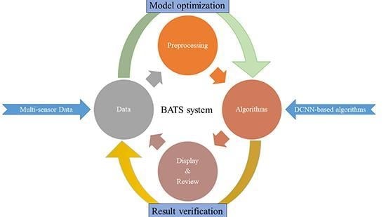
Different from the existing researches about the ship detection task, we not only focus on one specified algorithmic problem, but comprehensively consider various aspects existing in the task of the broad area ship detection, and then a processing chain of high-resolution data is established, named the broad area target search (BATS). In this framework, it includes image pre-processing, saliency estimation, scene mask estimation, ship detection, results presentation and manual review. The framework is shown in Figure 1, where a stack (or cube) indicates that the module contains several effective sub-steps, for example, the object detection step of BATS has some different implementations including the Saliency-Faster R-CNN, Faster R-CNN, FPN, etc.
Before elaborating on the details of each module in this framework, some explanations of the detection process will be given. Firstly, a remote sensing image with the resolution better than 1 m is called the high-resolution image in our method. Based on this resolution, we can get more information about the shape and context details of the ship, and these high-resolution images reflect multi-scale features of targets. It is also a main form of remote sensing data for the ship objects detection and a prerequisite for fine-grained identification. In BATS, each step operates on the high-resolution remote sensing images. Secondly, the step of the algorithms (D, E, F) in the flow chart can be executed independently to solve the specified problems during ship detection. Meanwhile, different methods can be selected according to characteristics of input data and the type of tasks. For example, step D and F can be used for the broad scene under the clouds without E. Finally, the data of the algorithms and system are all derived from a shared image database which is generated after data preprocessing. This database supports the data import, data and results storage for each step.
Now, we focus on the meaning of each step and the corresponding implementation process. The first is the input of data (Step A of Figure 1). In BATS, the high-resolution remote sensing data is obtained from Google Earth or uploaded from users. This is followed by the preprocessing of the raw data (Step B of Figure 1). For the high-resolution and wide coverage images, it is necessary to balance the size of the input image with the GPU performance. The most common processing method is to cut the input image into fixed-size patches (such as 1024×1024) for prediction. In order to ensure the integrity of the ship targets, we use an overlap cutting and overlap rate can be controlled. The data augmentation process includes some image operations such as multi-angle rotation, color contrast control and addition of random noise to increase the diversity of samples. The results of the preprocessing of input data are shown in Figure 2. For the structure management of the sample, the data is stored into the database after augmentation, which is convenient for the subsequent module.
After Step B, the database is utilized to store the real and public datasets separately for multiple utilization (Step C in Figure 1). In this database, the information of the training set and test set are stored in different tables. The information table of the training dataset contains the storage path, image size, file name, position in the original input, etc. The information table for the test dataset contains the storage path and processing results after testing.
In the following, the ship detection is illustrated from three aspects: Imaging factor, environmental factor and the ship target itself. First, for input scenes, the image quality should be further analyzed. In the task of the ship objects detection, the cloud occlusion has a huge impact on the target imaging. Severe cloud occlusion will directly lead to the blurring and disappearance of ship targets in this scene, as shown in Figure 3. Therefore, the effective measures should be taken to mitigate the cloud occlusion problem in such a scene (Step D of Figure 1). The usual algorithms for clouds removal mainly have two types: Physical model defogging and image enhancement for defogging. Among these methods, the typical physical model algorithm is the defogging in the dark channel based on the dark channel prior [36], and the most common traditional image enhancement is the contrast limited adaptive histogram equalization [37], in which by calculating the histogram of multiple local regions of the image to redistribute the brightness and contrast to realize defogging. With these effective defogging methods, the DCNN inside BATS can effectively classify the foggy scene from the fog-free scene, and then uses the classic algorithm to process the foggy images.
After defogging, the environment factors of the ship target are considered in Step E. In the task of ship detection, there are many ships mooring in ports or sailing in near-land areas. However, the complex terrestrial environment may easily mislead the feature extraction of DL algorithms and result in a lot of onshore false alarms. Therefore, there are some papers for ship detection that use sea-land separation to remove land false alarms. In this paper, we propose a novel false alarms suppression method based on DCNN, which use the powerful ability of feature extraction to segment the sea and land. The specific structure will be explained in Section 3.2.
The factors of the ship target itself should be focused to improve the ability of the ship targets detection (Step F of Figure 1). The size of the ship targets in the high-resolution remote sensing images varies greatly, while the size of the targets in the commonly used training dataset, such as DOTA [38], NWPU VHR-10 [39] and UCAS-AOD [40], are mostly similar and large-scale targets are rare, which results in a poor performance for large-scale ships detection. So far, some methods are proposed for concerning the problem of targets size, most of which use the combination of multi-layer feature layers [15,18,30] to retain the feature of different scale targets, and to alleviate the difficulty of the multi-scale targets detection. There is also a study that compresses the target in the image to a fixed size to enhance detection performance [17]. In our processing framework, a multi-scale ship detection method based on the saliency feature is proposed. This method adaptively compresses scenes containing large-scale ship targets, which improves the detection performance of remote sensing images in reality. The specific structure is explained in Section 3.3.
After ship detection, the result patches are aligned to the grid of the original image and the coordinates of the predicted boxes are converted into the original image coordinates. This step is known as data post-processing (Step G of Figure 1).
The post-processed data is stored in the database for the call of the display module. In the display module of BATS, the pixel coordinates of the predicted results are converted into geographic coordinates and the results are displayed in Google Map. In addition, the display module also provides an effective feedback mechanism, and that is the manual review for the ship detection algorithm (Step I of Figure 1). Considering that the DCNN-based methods cannot guarantee the detection result to be completely correct, the wrong result is selected manually and retrained to make up for the shortage of training samples, and then achieving the purpose of the iterative optimization of the algorithm. The structure and implementation of the display module will be explained in Section 4.3.
3. Ship Objects Detection Methods Based on DCNN
This chapter highlights the introduction of the DCNN-based ship detection algorithms proposed and applied in the BATS system which focuses on the onshore false alarm suppression and multi-scale ship object detection, respectively, in high-resolution remote sensing image. The first part would introduce the basic object detection network, which is used in both methods proposed in this paper. The second part would initially introduce the algorithm named as the Mask-Faster R-CNN focused on the problem that the near shore ship objects detection is disturbed by the onshore false alarms. This algorithm is combined with the scene mask extraction network that suppresses land information in feature maps to avoid the occurrence of onshore false alarms. Then, the algorithm concerning the problem of the multi-scale ship detection is demonstrated in the second part. In this method, a saliency estimation network is used to differentiate the scene containing large-scale objects from others, and then an image pyramid is used to compress these images so that the scale of the ships in real images is similar to the samples in the training dataset, and this improvement might have a good performance. Thus, this method is called the Saliency-Faster R-CNN.
3.1. Object Detection Network from Faster R-CNN
The object detection network adopts the classic two-stage detection process, which originated from the Faster R-CNN [14] by using ResNet-101 [41] as the feature extraction network (FEN) to implement the feature extraction of high-resolution remote sensing images. Then, the region proposal network (RPN) is used to conduct the candidate region proposal to obtain the high-confidence region proposals and corresponding coordinates on the feature map obtained by FEN. At last, it puts the region proposal and corresponding feature map through ROI pooling operation [14] to obtain the feature map block in the fixed size, then the classification and regression of the region proposal calculated by RPN is conducted to obtain a more accurate object class and coordinates and thus this process is known as the classification and regression network (CRN). The structure of the object detection network is shown in Figure 4.
The ResNet-101 network is made up of 99 convolutional layers, which consist of four ResNet blocks [41] and two fully-connected layers. Due to its special block structure, it could extract the deep feature in the image without the problem of the vanishing gradient, which makes it extremely appropriate for feature extraction of ship objects in the complicated environment. In order to import this network into the object detection network, we remove the last two fully-connected layers and divide it into two parts: The first part is used as the FEN, which include the first three ResNet blocks and the second part (the fourth ResNet block) is used after the operation of the ROI pooling. The configuration of FEN is shown in part one of Table 1 and the configuration of another block in part two.
In the object detection network, the most important structure is the RPN, which is used to propose regions that have a high-confidence and are closer to the ground-truth of targets by using some fixed-size anchors [14]. However, this process is controlled by the training dataset and the loss of classification and regression, which means the region proposal mechanism of RPN relies on the samples in the dataset. Therefore, it is hard to differentiate the objects with similar characteristics of targets in the non-target area. Furthermore, assuming that there are many small-scale objects in our training dataset, RPN is restrained so that it only responds to the small-scale targets while the large-scale targets cannot be fully covered by the insufficient anchors. Theoretically, the anchors and the subsequent regression process in the RPN prefers to fit the small-scale objects, and thus the large-scale targets are ignored via the trained RPN. The mechanism of RPN is shown in Figure 5. After RPN, a ROI pooling operation is used to resize all region proposals with 14×14 (same with the input of the fourth block in ResNet-101). Then, the feature in each proposal is used to finish the classification and regression to get the target class and coordinates.
3.2. Mask-Faster R-CNN for Suppression of Onshore False Alarms
In the ship detection process, because of the complexity of the land surface, there are amounts of objects that have a similar feature with the ships, which results in the fact that these objects might be regarded as candidate objects and influences the accuracy of the DL algorithm. Therefore, in terms of the problem of onshore false alarms, we put forward a ship detection method based on the estimated scene mask, known as the Mask-Faster R-CNN. This method could assist the object detection network by knowing target and non-target areas. Then, the region proposals are obtained only in the target area by using RPN and classified by using the softmax classifier to eventually implement the detection of the ship objects. As a mechanism to accurately judge the region proposals, the estimated scene mask could be used to suppress false alarms in the non-target area, such as harbor area and island, which reduces the redundancy of the region proposals, and eventually increases the accuracy of detection. The flow chart of the training process is shown in Figure 6.
The Mask-Faster R-CNN consists of four sub-networks: The FEN based on Resnet-101, its parameters is presented in Table 1; a branch of the scene mask extraction network (SMEN) is inserted to estimate the scene mask by using the deconvolution operation; the RPN and CRN are used to decide the class and coordinates of the targets. Additionally in this method, the key point of suppressing the onshore false alarms is to eliminate the information of the non-target area (i.e., land) which is realized by SMEN.
3.2.1. Scene Mask Extraction Network
In this method, the role of the scene mask extraction network is a pixel-level classification between the target area (sea) and non-target area (land) to eliminate the disturbance of the non-target area in the forward propagation stage, which is the core idea in the onshore false alarm suppression. Since the boundaries of shores, especially in the harbor area, usually appear to be irregular and have a variety of shapes, it is necessary to classify each pixel in the input image in order to achieve accurate segmentation results. Deconvolution is an up-sample mechanism, which could operate the convolution process and restore the original size of the image at the mean time. By using the combination of the convolution, down-sample and deconvolution operations [42], we could implement the classification on each pixel (i.e., semantic segmentation in the context of DL). Therefore, the function of SMEN is a separation of the sea and land. At first, the scene label is introduced as a binary mask between the target and non-target areas in our dataset. Next, we add four deconvolution layers after FEN, and then the intermediate feature map goes through a softmax layer, which calculates the result of the non-target area (i.e., land scene). Additionally, the configuration of SMEN is shown in Table 2.
Considering the real circumstance, for example the harbor area, parked ships are common near the shore, a low accuracy in boundary segmentation would result in the problem that the sea area may be classified as the land by mistake, which makes the detection stage abandon the ship targets covered by this inaccuracy land mask. In order to effectively extract the scene mask and avoid disturbing the parked ship objects, it is necessary to further optimize the accuracy in the segmentation. Therefore, the low-level feature map of SMEN is imported into the deconvolution layer by using the concatenate operation to optimize the accuracy of the estimated scene mask. To elaborate, the specific method is to concatenate the outcome feature map of each block in FEN with the same-size deconvolution layer, and then put the concatenated feature map through a convolutional layer in order to implement a further feature extraction. According to the operations above, a more accurate boundary information and more abstract semantic information are presented in the high-level feature map.
3.2.2. Training Process
In the training process, a multi-task loss function is established to restrain the training. The loss function is calculated by forward propagating in each iteration, and the parameters in all sub-networks are updated by using the gradient descent method [5]. When the minimum of the loss function is obtained, eventually the network is convergent.
The loss function of SMEN, denoted by , could be represented as the cross entropy of the scene mask obtained in the network and ground truth label for each training image, and the expression is shown by Formula (1).
where is the size of the scene mask, is the prediction probability of the scene category of the pixel in the image, and , is the ground truth of the pixel with the value of zero and one, representing the scenes of the land and sea, respectively, and the size of the image is .
The loss function of classification in the object detection network could be represented as the cross entropy of the classification outcome and its ground truth, which is denoted by , as shown in Formula (2):
where is the predicted probability being a target of box , is ground truth of the target, and it equals one when the label is positive, and is zero when the label is negative. is the number of boxes.
The loss function of the bounding box regression could be represented as the , which is the entropy loss between the region proposals and the ground truth box closest to it, denoted by , as shown in Formula (3) and Formula (4).
where is the number of box locations, is utilized to balance the process of classification and regression. is the vector containing four coordinates of bounding boxes obtained by the object detection network, and represents the coordinates of the ground truth boxes.
The total loss function of Mask-Faster R-CNN is the weighted sum of the three loss functions, as shown in Formula (5).
where and are hyper-parameters to balance the loss of classification, regression and mask estimation.
3.2.3. Inference Process
There is a considerable difference between the inference and training process. The scene mask estimation and the object detection are driven by the above training, however, without any information interaction, while in the inference process, the outcome of the scene mask extraction network needs to exert an impact on the object detection network. Initially, the input image goes through the FEN and SMEN to obtain the information that represents the scene mask, which is a binary matrix with the value of one for the target area and zero for the non-target area.
where is the estimated scene mask with the value of zero or one obtained from SMEN, and the is a set of pixels belonging to the non-target area (i.e., land).
Then, after compressing this scene mask into the size of the final feature map, i.e., the output of FEN with channels, it will be multiplied with each channel of the feature map obtained from FEN, which would set the value of the non-target area in the feature map to zero, eliminating the effect of this area in the subsequent RPN process. In addition, this process can be formulated as:
where represents the Hadamard product, and is a certain channel of the feature map obtained from FEN. Then is employed in the RPN to effectively reduce the false alarms in the non-target area, and the inference framework is shown in Figure 7.
3.3. Saliency-Faster R-CNN for Multi-Scale Ship Detection
It is usually difficult to get rid of the influence from the training dataset pattern in the object detection task by using the DL algorithm, and unfortunately, the same problem more obviously exists in the ship object detection in a high-resolution image. Most of the available training samples of the ship reflect the small-scale targets, which leads to the fact that the DL algorithm could not correctly learn the feature of the multi-scale ships, especially some large ships. In other words, the trained DCNN may be limited by the small-scale ships in the training dataset. Therefore, it is necessary to adopt an effective scale adjustment mechanism to implement the accurate multi-scale ship detection. On account of the difference between the training dataset and the real scene with the large ship, an object detection method based on the saliency estimation network, known as the Saliency-Faster R-CNN, is proposed in this paper which combines the object detection network with the saliency estimation network. By making use of the saliency estimation network to describe the object scale of remote sensing images, it divides inputs into the scene with the large-scale object and the scene with the small-scale object. Based on this division, it constructs an image pyramid to compress the images and adjust the input close to the sample scale and increases the detection ability of the object detection network for multi-scale ships (large-scale object, especially). The overall framework of the network is shown in Figure 8, where the object detection network has been described in the Mask-Faster R-CNN.
3.3.1. Saliency Estimation Network
In the Saliency-Faster R-CNN, the purpose of the saliency object network is to extract the saliency feature of the object and further distinguish the scenes containing large-scale or small-scale objects. Since the current DL algorithm is considerably dependent on the pattern of the samples, it is difficult to effectively implement the large-scale object detection task in some real scenes by using the small-scale object dataset. Therefore, we adopt the traditional digital image processing method to construct the saliency estimation network, which could extract the saliency feature of objects.
In this saliency estimation network, we first process the high-resolution remote sensing image and obtain the saliency feature of ships by using the saliency estimation algorithm. Based on this, the gray values in the saliency map obtained after the saliency estimation are analyzed by using the histogram method, and then estimating the saliency degree of the ship scale. Second, combined with the statistical results, we construct a mathematical model which could distinguish the large-scale ship and small-scale ship scenes. The framework of the saliency estimation is shown as the input in Figure 8.
It is worth noting that there are many saliency estimation algorithms, and thus we studied the ability of different saliency estimation algorithms for high-resolution images. Comparing and analyzing the performance in real high-resolution images of several classic algorithms which can be found in [43], including Saliency Intensity Model (SIM) [44], region Covariance (COV) [45], Fast and Efficient Saliency detection (FES) [46], Segmenting object detection (SEG) [47], Spectral Residual approach (SR) [48], Saliency Using Natural statistics [49], Spatially Weighted Dissimilarity (SWD) [50], and the SIM is assured as the algorithm adopted in saliency estimation network. The saliency map outcome and histograms analyzing the outcome are shown in Figure 9.
According to Figure 9, we could infer that the results of the SIM algorithm are able to appropriately present the energy distribution of objects in the high-resolution remote sensing image, and could effectively distinguish the scenes whether containing the large-scale ships or not. The describing factor of the target scale is shown in Formula (8).
where represents the statistical feature information, and , represent the upper and lower bounds of left peak in the histogram, and are also boundaries of the gray interval for the right peak, and is the threshold. When , the input image is interpreted as a scene with large-scale ships. It is found in the experiment that the area with the low gray value in the saliency map is related to the background information, while the area with a high value is related to the object information. It is worthy to note that this series of parameters are estimated in the ship detection process, so it should be adjusted dealing with the size of the input image in different circumstances.
3.3.2. Training and Inference
In the training process, the saliency estimation network is operated by the traditional processing method, it is not necessary to train on a specific dataset. Therefore, there is no need to participate in the training process. Thus, the total loss function is made of the weighted sum of the bounding box loss function and classification loss function, and the expression is shown in Formula (9).
where and are elaborated in formula (2) and (3), and is a hyper-parameter to balance the loss of classification and regression.
In the inference process, based on the saliency map obtained by the saliency estimation, the scenes including large-scale ships or small-scale ships are distinguished. Combining with the mechanism of the image pyramid, it achieves the compression of images including large-scale ships, and implements the scale consistency of ships between real scenes and training samples. Then, it imports the compressed images into the object detection network to conduct the ship objects detection.
4. The Construction of the BATS System
This part will mainly introduce the structure, function and display interface of the BATS system, which belong to Step A, Step H and Step I of Figure 1, respectively. Each interface in the front end is inseparable from the architecture of the system function. It is an essential tool for the human-computer interaction and an effective measure to enhance performance. Aiming to detect ships over a broad area automatically, by using high-resolution remote sensing images collected from Google Earth or uploaded by users, a visual and interactive system, i.e., BATS, is developed based on the WEB technology and DL model.
The BATS has two work components: The front end and back end. The front end is developed based on the Vue.js framework [51] and combined with Google Map API [52] for the data input and data display. The back end is developed based on Django [53] and uses SQLite [54] as the database. The service of the back end includes the database interaction, image preprocessing and calling DL models. Figure 10 shows the architecture of the BATS system.
4.1. Broad Area Search Module
The broad area search module is the main function in BATS for ship detection in the wide coverage and high-resolution remote sensing images. In this module, we use the wide areas in Google Earth as an instance to display the detection results (Step A and Step H in Figure 1). The interface of the broad area search module is shown in Figure 11.
As illustrated in Figure 11, on the left side of this interface, there is a window displaying high-resolution remote sensing image with wide coverage, and this broad area has many regular areas of interest (AOIs), in which the user can scan and select one or more AOIs to search the ships. After clicking the search button, the red markers of the targets are shown in this window and the thumbnails of the predicted results of the cropped images are displayed in the right side of the interface. The user can click on the thumbnail to view the image details.
The realization process of this module is as follows: (1) A broad region on Google Map is divided into several large regular AOIs which correspond to some remote sensing images. (2) Users select the AOIs to search ship targets. (3) The system begins pre-processing (format conversion, image segment) the corresponding images, and calls the DL model for ship detection, and records the position of the marked targets. (4) The markers of the targets and thumbnails of the predicted results will be displayed on the page. The data flow of the broad area search module is shown in Figure 12
4.2. Target Detection Module
The target detection module is mainly to meet the inference requirements of individual images (Step A and Step H in Figure 1). The interface of the target detection module is shown in Figure 13. There is the upload file function located on the left side of this page, in which the user can drag a single image or folder into the box to upload. The results of the inference will be displayed by the carousel on the right side of the page, and the user can switch the current displayed images.
In the target detection module, we first determine whether the type and size of the uploaded images are correct and call the pre-processing procedure and DL models for the ship target detection. Finally, the results of detection are displayed in the web page. The data flow in the target detection module is same as Figure 12.
4.3. Manual Review Module
The purpose of the manual review module is to artificially inspect the results after inference, which is relative to step I in the architecture of BATS. In fact, it is necessary to conduct a manual review because the problems inside the network are directly reflected on these results, and this could give us a lot of chances to develop effective improvements.
The interface of the manual review module is shown in Figure 14. There is a presentation area on the left side of this page, in which the user can preview the result image and then vote for problems contained in this image shown on the right side. After that, the result with an error will be stored into the database for the process of subsequent relabeling and training. During the steps of the manual review, the data flow is shown in Figure 15.
5. Results
This section is devoted to present the results of the different DCNN-based algorithms on their aspects of concern and the results of the entire system in the real high-resolution remote sensing image. During the experiment, the validity is carried out by using the same infrastructure and evaluation indicators, then, we analyze the result and compare it to baseline method, i.e., the Faster R-CNN, to validate the effectiveness of our methods. At last, some additional discussions about the system application environment and scene are presented.
5.1. Introduction of Dataset
In this paper, DOTA [38] is utilized as the training dataset, and the resolution of most images in this dataset is better than 1 m. In DOTA, there are 434 scenes of different sizes containing multi-scale ships, it is fortunate that this distribution, i.e., small-scale ships occupy the majority of the dataset and most of them are close to the harbor in these scenes as shown in Figure 16, accords with the problems that have been solved in this paper. Eventually, 400 images are obtained from the dataset by manual selection (excluding the relative low-resolution images) and labeled with mask information in order to be able to train in both proposed DCNN algorithms. The background information and target categories of these images are complex, which include the different lighting conditions and cloud occlusions, and the dataset contains a variety of ship categories such as the cargo, cruise, carriers, etc. It ensures the diversity of the samples.
The testing dataset consists of some images randomly picked from DOTA, and some remote sensing images collected from Google Earth are chosen as the testing images, in which the resolution is 0.3 m. Therefore, the images with labeled targets in our dataset are shown in Figure 17, in which the green box represents the ground truth of the ship target, and the white part represents the land (i.e., non-target) area while the black one is the sea in the mask map of the ground truth.
In order to keep the consistency of the input in networks and the effective training process under one GPU, the images in the dataset are cut into the fixed size of 1024×1024 with a 20% overlap rate, and thus more than 1600 images are generated in the pre-processing step. Then, the images from DOTA are split into the training data and testing data with the rate of 8:2. Eventually, we form the testing dataset by merging about 310 images from the DOTA testing data and 152 images collected from Google Earth after pre-processing. Further, the augmentation operations have been operated to improve the generalization ability of networks.
All models are built on a Tensorflow DL framework and calculated on the GeForce GTX 1080 Ti GPU. As a result of the same structure of RPN in both proposed networks, we set its parameters to be the fixed value that the scale is in (4, 8, 16, 32, 64) and the aspect ratio is in (0.5, 1, 2). Additionally, all models are trained with the initial weight value based on ResNet-101 and overall training steps are 80,000.
5.2. Results of Multi-Scale Ship Detection
A set of comparison experiments has been conducted in this part, which compares the Saliency-Faster R-CNN proposed in this paper to the baseline method (Faster R-CNN) to validate the accuracy and superiority of our method. In fact, SVM [55], as a classic machine learning method, can also be combined with DCNN for classification, however, relevant studies have proved that the classification accuracy of SVM is slightly less than the softmax used in the Fast R-CNN [13], Faster R-CNN [14] and Bengio’s research [56], in addition, the method based on SVM is not an end-to-end system, that is the reason for choosing Faster R-CNN as the benchmark method in our paper. In these experiments, we select the images containing the large-scale ship as an independent dataset to highlight the advantages of our method, and during the testing process, we adopt , , , and to calculate the describing factor of the target scale (see Formula (8)). The value of the average precision (AP) is used to indicate the performance of detection results, which is shown in Table 3. The value of APL represents the AP index on the large-scale ship dataset. The NCR (not compressing rate) represents the rate of failure to differentiate the ship size, i.e., not properly compressing the input image containing the large-scale ships, during the process of saliency estimation.
It should be noted that the AP of the ship by using the Faster R-CNN is only 0.504 in the literature of the first proposed DOTA [38], but our baseline method here has a value of 0.606, the reason for the improvement of accuracy is not only the effectiveness of our processing but the single category detection in our experiments. In Table 3, the APL of the Saliency-Faster R-CNN is 0.727, which is much better than APL of the Faster R-CNN, and it is more obvious than the improvement in AP. Actually, this is a reasonable result because the number of large-scale ships in the dataset is much less than the others, it is hard to promote a lot on AP. Therefore, on the basis of maintaining the detection accuracy of small-scale ships, our method also has a significant improvement on the detection of large-scale ships, which is an important aspect in the ship detection task by using the high-resolution remote sensing image.
Furthermore, according to the result in Table 3, the NCR of the Saliency-Faster R-CNN is only 0.105, which fully demonstrates the effectiveness of the saliency estimation. Some testing images and their saliency maps are shown in Figure 18. The intuitive detection results of the baseline and our method are shown in Figure 19, and it is obvious that the large-scale ships can be accurately detected after the compressing process in our method.
5.3. Results of Onshore False Alarm Suppression
In order to validate the accuracy of the Mask-Faster R-CNN, the experiment between the Faster R-CNN and our method has been realized. AP, utilized in the above experiment, and two extra indicators known as the false rate and mean intersection over union (mIOU) are introduced to evaluate the detection results. The assessment is presented in Table 4, where the false rate indicates the false alarm rate in the detection results, and the mIOU demonstrates the performance of the scene mask estimation in the Mask-Faster R-CNN.
In Table 4, the AP of the Mask-Faster R-CNN is 0.628, which is 2.2% higher than that of the Faster R-CNN, and at the same time, the value of the false rate has a huge reduction from 0.686 to 0.397. Obviously, when the land (non-target area) information is reduced during the detection process, some improvements on the false alarm and accuracy are obtained. This also demonstrates that our method can effectively suppress the onshore false alarms and promote the nearshore ship detection. Furthermore, we get a value of 0.877 on mIOU, which means the scene mask predicted in the inference process is very similar to the ground truth, and it can prove that this network is able to differentiate the target area (sea) and non-target area (land). Some inference results of the Faster R-CNN and Mask-Faster R-CNN are shown in Figure 20, in which the yellow region represents the predicted scene mask, the red boxes represent the ship detection results, and the blue boxes represent the existing false alarms. In these results, the Mask-Faster R-CNN effectively reduces the number of onshore false alarms.
6. Discussions
The above experiments are designed to analyze the accuracy of two DCNN models independently. Then in this part, an analysis on the effectiveness of the system and cascading model (connecting the Saliency-Faster R-CNN with Mask-Faster R-CNN) is presented. First, the results of the cascading model are compared with each DCNN model separately to validate the accuracy and effectiveness of the cascading model. The evaluation results of the different models are shown in Table 5, where time represents the average inference time on each image with 1024 × 1024.
According to Table 5, the AP of the cascading mode (the fourth row) is 0.629, which has a little improvement compared with the Mask-Faster R-CNN, and it indicates that the cascading model really fuses the advantages of two DCNN models proposed in this paper. However, the consumption time of both the DCNN model is larger than that of the Faster R-CNN, which only has 0.173 sec/image, while the time of the Saliency-Faster R-CNN reaches 2.181 sec/image because of the saliency estimation in this network, so that the time of the cascading model even reaches 2.233 sec/image. Objectively speaking, this is unbearable in real-time detection tasks of massive data, but it still can be used as a time-accuracy balance choice because of its improvement on the large-scale ship detection.
Then, an evaluation of the efficiency on the entire system is conducted by using some high-resolution remote sensing images not in the testing data set. The environment of evaluation consists of one GPU, a communication network with 1000 Mbps, one CPU with quad core and eight threads. The results are shown in Table 6.
In Table 6, the upload represents the time consumption when uploading the images by the site designed in this paper, the pre-processing represents the time consumed in pre-processing, which includes images cutting with the fixed size and its position record in the original image, the post-processing represents the time consumed by dealing with the results after the detection process, which includes the coordinates transformation of boxes in the original images, the removal of repeated detection results by using the NMS operation in the overlapping area, finally the Num of Images represents the total number of images by using the overlapping cutting. According to statistics in Table 6, the times of processing and transferring are very short compared to the detection time, it will not influence the efficiency of the entire system and can be accepted.
In addition, in order to demonstrate the superiority of the cascading model and each individual model on different conditions, the curve of the precision-recall (PR) for each DCNN model is drawn in Figure 21.
From Figure 21, in the same value of the recall, the precision from high to low is the cascading model, Mask-Faster R-CNN, Saliency-Faster R-CNN and Faster R-CNN. The result indicates that not only our two individual models can improve the accuracy of ship detection on their respective different concerns but the cascading model has a comprehensive improvement because of its fusion of two DCNN models.
In addition to the harbor scenes, we have encountered some scenes which contain icebergs located in the Arctic, and it is frequent to be some false alarms near or on iceberg during ship detection. Fortunately, our method still has a good performance on these scenes. Some results are shown in Figure 22, and the Faster R-CNN is deteriorated because of the false alarms, however, the Mask-Faster R-CNN avoids such a problem by using the estimated scene mask. In order to prove the applicability ability of BATS, we uploaded some high-resolution panchromatic remote sensing images via the target detection module, which are obtained from Gaofen-2 (GF-2) and the resolution of images is 0.8 m, and the results are shown in Figure 23. It is obvious that our method still has a good performance compared with the Faster R-CNN, even the type of input data is different from our training set. The generalization performance of the proposed system is verified to some extent.
Finally, one broad-area high-resolution remote sensing image is used to demonstrate the effectiveness and accuracy of our BATS for the complex scene. The size of the input image is 10656 × 7130, which is collected from Google Earth and it is one part of the Norfolk harbor, and the resolution of image is 0.3 m, which means it can nearly present a Nimitz-class aircraft carrier. The detection result is shown in Figure 24.
It can be seen that in (a) of Figure 24 almost each ship can be exactly detected in this complex scene, and some huge ships, for example the Nimitz-class aircraft carrier close to the harbor, which is shown in (e), can be marked through the Saliency-Faster R-CNN. Meanwhile, a dense ships scene is located on the right side of the image, and its scaled up image is shown in (b), and each small-scale ship has been detected, and it is amazing that some onshore alarms are suppressed, which means our Mask-Faster R-CNN plays its role in the system. At the same time, (d) and (f) obtained from the Faster R-CNN are the contrast of (c) and (e), respectively, which indicates that our method suppresses the onshore false alarms and detect the large-scale ship. Therefore, the BATS system has a good detection performance on the broad area.
7. Conclusions
In order to implement the DCNN-based ship detection in the broad area by using high-resolution remote sensing images, a ship detection system consisting of data pre-processing, core algorithms based on DCNN, results display module and manual review module is proposed in this paper, known as the broad area target search (BATS) system. The ship detection algorithms in this system are the key step in the ship detection task. For the problem of object scale differences between the training dataset and real scenes, a method known as the Saliency-Faster R-CNN combining the saliency estimation network with the object detection network is proposed in this paper, which uses the saliency feature to describe the scale of the ship inside the image, then the image pyramid is utilized to compress the input image that includes the large-scale objects so that the ship scale in the real high-resolution image is close to the scale of samples in the training dataset, and eventually it improves the detection accuracy. Additionally for the problem of onshore false alarms, a method named as Mask-Faster R-CNN is introduced, which inserts a branch of the scene mask estimation network into the object detection network to learn how to discriminate the target area (sea) from the non-target area (land), and then cover the land area with a zero response during the RPN process. This method can effectively reduce the appearance of onshore false alarms.
Furthermore, this system also incorporates the capabilities of the data structure management of database technology to realize the results storage and display of each step inside the system, and meantime, it also provides users an interface to review the results and iteratively optimize the core DCNN-based algorithms. The processing chain based on the database unit constitutes an important foundation of the data interaction between the BATS system and users.
Through the independent experiment of each DCNN algorithm, the validity of each part has been verified. Firstly, we validate the Saliency-Faster R-CNN and obtain its superiority compared to the Faster R-CNN on the large-scale ship detection. Then, the Mask-Faster R-CNN is verified to have its greatly improvement compared to the Faster R-CNN on the suppression of onshore false alarms. In the last part, two DCNN-based algorithms are combined to validate the accuracy and efficiency of the entire system. Actually, the results are really satisfied either on the independent experiment or on the cascade experiment. To summarize, the framework proposed in our research provides a series of effective solutions for ship detection in the high-resolution remote sensing image.
At last, taking the data-driven and complexity of the ship detection task into account, the scalability of the BATS system is increased by using the database and the way of algorithm cascading so that it inserts more DCNN-based algorithms and constantly improves the performance of ship detection. In future work, some targets of interest in high-resolution remote sensing images, such as the airplane, vehicle, storage tank etc., will be concerned in the BATS system. The DCNN models proposed in this paper need to be continuously optimized according to the diversity of targets and scenes in the detection task. Furthermore, considering the all-time and all-weather capability of the synthetic aperture radar (SAR) images, it can be used as a powerful complement to the optical remote sensing images to achieve an accurate target detection under the condition of the heavy cloud and fog and inadequate optical data.
Author Contributions
Conceptualization, Y.Y. and Z.L.; Methodology, Y.Y., Z.L., B.R. and J.C.; Software, B.R. and Z.L.; Validation, Z.L., B.R., J.C. and S.L.; Formal analysis, Z.L.; Investigation, Y.Y. and Z.L.; Resources, Z.L.; Data curation, Z.L.; Writing—original draft preparation, Y.Y., Z.L., B.R. and S.L.; Writing—review and editing, Y.Y. and Z.L.; Visualization, Z.L. and B.R.; Supervision, Y.Y. and F.L.; Project administration, Y.Y.;
Funding
“Fundamental Research Funds for the Central Universities” (2018RC09).
Acknowledgments
This work is conducted on the platform of the Center for Data Science of Beijing University of Posts and Telecommunications.
Conflicts of Interest
The authors declare no conflict of interest.
References
- Kanjir, U.; Greidanus, H.; Oštir, K. Vessel detection and classification from spaceborne optical images: A literature survey. Remote Sens. Environ. 2018, 207, 1–26. [Google Scholar] [CrossRef] [PubMed]
- Bishop, C.M. Pattern Recognition and Machine Learning; Springer: Berlin/Heidelberg, Germany, 2006. [Google Scholar]
- Dalal, N.; Triggs, B. Histograms of oriented gradients for human detection. In Proceedings of the International Conference on Computer Vision & Pattern Recognition (CVPR’05), San Diego, CA, USA, 20–25 June 2005; Volume 1, pp. 886–893. [Google Scholar]
- Papageorgiou, C.P.; Oren, M.; Poggio, T. A general framework for object detection. In Proceedings of the 6th International Conference on Computer Vision (IEEE Cat. No. 98CH36271), Bombay, India, 7–7 January 1998; pp. 555–562. [Google Scholar]
- Goodfellow, I.; Bengio, Y.; Courville, A. Deep Learning; MIT press: Cambridge, MA, USA, 2016. [Google Scholar]
- Haykin, S. Neural networks: A Comprehensive Foundation; Prentice Hall PTR: Upper Saddle River, NJ, USA, 1994. [Google Scholar]
- Krizhevsky, A.; Sutskever, I.; Hinton, G.E. Imagenet classification with deep convolutional neural networks. In Proceedings of the Advances in Neural Information Processing Systems, Lake Tahoe, NV, USA, 3–6 December 2012; pp. 1097–1105. [Google Scholar]
- Viola, P.; Jones, M. Others Rapid object detection using a boosted cascade of simple features. CVPR 2001, 1, 511–518. [Google Scholar]
- Long, J.; Shelhamer, E.; Darrell, T. Fully convolutional networks for semantic segmentation. In Proceedings of the IEEE Conference on Computer Vision and Pattern Recognition, Boston, MA, USA, 7–-12 June 2015; pp. 3431–3440. [Google Scholar]
- Boutell, M.R.; Luo, J.; Shen, X.; Brown, C.M. Learning multi-label scene classification. Pattern Recognit. 2004, 37, 1757–1771. [Google Scholar] [CrossRef] [Green Version]
- Girshick, R.; Donahue, J.; Darrell, T.; Malik, J. Rich feature hierarchies for accurate object detection and semantic segmentation. In Proceedings of the IEEE Conference on Computer Vision and Pattern Recognition, Columbus, OH, USA, 24–27 June 2014; pp. 580–587. [Google Scholar]
- Uijlings, J.R.; Van De Sande, K.E.; Gevers, T.; Smeulders, A.W. Selective search for object recognition. Int. J. Comput. Vis. 2013, 104, 154–171. [Google Scholar] [CrossRef]
- Girshick, R. Fast r-cnn. In Proceedings of the IEEE International Conference on Computer Vision, Washington, DC, USA, 2015, 7–13 December; pp. 1440–1448.
- Ren, S.; He, K.; Girshick, R.; Sun, J. Faster r-cnn: Towards real-time object detection with region proposal networks. In Proceedings of the Advances in Neural Information Processing Systems, Montréal, QC, Canada, 7–12 December 2015; pp. 91–99. [Google Scholar]
- Lin, T.-Y.; Dollár, P.; Girshick, R.; He, K.; Hariharan, B.; Belongie, S. Feature pyramid networks for object detection. In Proceedings of the IEEE Conference on Computer Vision and Pattern Recognition, Honolulu, HI, USA, 21–26 July 2017; pp. 2117–2125. [Google Scholar]
- He, K.; Gkioxari, G.; Dollár, P.; Girshick, R. Mask r-cnn. In Proceedings of the IEEE International Conference on Computer Vision, Venice, Italy, 22–29 October 2017; pp. 2961–2969. [Google Scholar]
- Singh, B.; Davis, L.S. An analysis of scale invariance in object detection snip. In Proceedings of the IEEE Conference on Computer Vision and Pattern Recognition, Salt Lake City, UT, USA, 18–22 June 2018; pp. 3578–3587. [Google Scholar]
- Liu, W.; Anguelov, D.; Erhan, D.; Szegedy, C.; Reed, S.; Fu, C.-Y.; Berg, A.C. Ssd: Single shot multibox detector. In European Conference on Computer Vision; Springer: Berlin/Heidelberg, Germany, 2016; pp. 21–37. [Google Scholar]
- Redmon, J.; Divvala, S.; Girshick, R.; Farhadi, A. You only look once: Unified, real-time object detection. In Proceedings of the IEEE Conference on Computer Vision and Pattern Recognition, Las Vegas, NV, USA, 26 June–1 July 2016; pp. 779–788. [Google Scholar]
- Redmon, J.; Farhadi, A. Yolov3: An Incremental Improvement. arXiv 2018, arXiv:180402767. [Google Scholar]
- Daniel, B.J.; Schaum, A.P.; Allman, E.C.; Leathers, R.A.; Downes, T.V. Automatic ship detection from commercial multispectral satellite imagery. In Algorithms and Technologies for Multispectral, Hyperspectral, and Ultraspectral Imagery XIX; International Society for Optics and Photonics: Bellingham, WA, USA, 2013; Volume 8743, p. 874312. [Google Scholar]
- Kanjir, U.; Marsetič, A.; Pehani, P.; Oštir, K. An automatic procedure for small vessel detection from very-high resolution optical imagery. In Proceedings of the 5th GEOBIA, Thessaloniki, Greece, 21–24 May 2014; pp. 1–4. [Google Scholar]
- Buck, H.; Sharghi, E.; Bromley, K.; Guilas, C.; Chheng, T. Ship detection and classification from overhead imagery. In Applications of Digital Image Processing XXX; International Society for Optics and Photonics: Bellingham, WA, USA, 2007; Volume 6696, p. 66961C. [Google Scholar]
- Lavalle, C.; Rocha Gomes, C.; Baranzelli, C.; Batista e Silva, F. Coastal Zones Policy Alternatives Impacts on European Coastal Zones 2000–2050; JRC Technical Note; European Union: Brussels, Belgium, 2011; p. 64456. [Google Scholar]
- Jin, T.; Zhang, J. Ship detection from high-resolution imagery based on land masking and cloud filtering. In Seventh International Conference on Graphic and Image Processing (ICGIP 2015); International Society for Optics and Photonics: Bellingham, WA, USA, 2015; Volume 9817, p. 981716. [Google Scholar]
- Li, N.; Zhang, Q.; Zhao, H.; Dong, C.; Meng, L. Ship detection in high spatial resolution remote sensing image based on improved sea-land segmentation. In Hyperspectral Remote Sensing Applications and Environmental Monitoring and Safety Testing Technology; International Society for Optics and Photonics: Bellingham, WA, USA, 2016; Volume 10156, p. 101560T. [Google Scholar]
- Xu, J.; Sun, X.; Zhang, D.; Fu, K. Automatic detection of inshore ships in high-resolution remote sensing images using robust invariant generalized Hough transform. IEEE Geosci. Remote Sens. Lett. 2014, 11, 2070–2074. [Google Scholar]
- Beşbinar, B.; Alatan, A.A. Inshore ship detection in high-resolution satellite images: Approximation of harbors using sea-land segmentation. In Image and Signal Processing for Remote Sensing XXI; International Society for Optics and Photonics: Bellingham, WA, USA, 2015; Volume 9643, p. 96432D. [Google Scholar]
- Burgess, D.W. Automatic ship detection in satellite multispectral imagery. Photogramm. Eng. Remote Sens. 1993, 59, 229–237. [Google Scholar]
- Yang, X.; Sun, H.; Fu, K.; Yang, J.; Sun, X.; Yan, M.; Guo, Z. Automatic ship detection in remote sensing images from google earth of complex scenes based on multiscale rotation dense feature pyramid networks. Remote Sens. 2018, 10, 132. [Google Scholar] [CrossRef]
- Jiang, Y.; Zhu, X.; Wang, X.; Yang, S.; Li, W.; Wang, H.; Fu, P.; Luo, Z. R2cnn: Rotational Region Cnn for Orientation Robust Scene Text Detection. arXiv 2017, arXiv:170609579. [Google Scholar]
- Yang, X.; Sun, H.; Sun, X.; Yan, M.; Guo, Z.; Fu, K. Position detection and direction prediction for arbitrary-oriented ships via multitask rotation region convolutional neural network. IEEE Access 2018, 6, 50839–50849. [Google Scholar] [CrossRef]
- Zhang, R.; Yao, J.; Zhang, K.; Feng, C.; Zhang, J. s-cnn-based ship detection from high-resolution remote sensing images. Int. Arch. Photogramm. Remote Sens. Spat. Inf. Sci. 2016, 41. [Google Scholar]
- Bodla, N.; Singh, B.; Chellappa, R.; Davis, L.S. Soft-NMS–Improving Object Detection with One Line of Code. In Proceedings of the IEEE International Conference on Computer Vision, Venice, Italy, 22–29 October 2017; pp. 5561–5569. [Google Scholar]
- Yang, X.; Fu, K.; Sun, H.; Yang, J.; Guo, Z.; Yan, M.; Zhan, T.; Xian, S. R2CNN++: Multi-Dimensional Attention Based Rotation Invariant Detector with Robust Anchor Strategy. arXiv 2018, arXiv:181107126. [Google Scholar]
- He, K.; Sun, J.; Tang, X. Single image haze removal using dark channel prior. IEEE Trans. Pattern Anal. Mach. Intell. 2010, 33, 2341–2353. [Google Scholar]
- Reza, A.M. Realization of the contrast limited adaptive histogram equalization (CLAHE) for real-time image enhancement. J. VLSI Signal Process. Syst. Signal Image Video Technol. 2004, 38, 35–44. [Google Scholar] [CrossRef]
- Xia, G.-S.; Bai, X.; Ding, J.; Zhu, Z.; Belongie, S.; Luo, J.; Datcu, M.; Pelillo, M.; Zhang, L. DOTA: A large-scale dataset for object detection in aerial images. In Proceedings of the IEEE Conference on Computer Vision and Pattern Recognition, Salt Lake City, UT, USA; 2018; pp. 3974–3983. [Google Scholar]
- Cheng, G.; Han, J.; Zhou, P.; Guo, L. Multi-class geospatial object detection and geographic image classification based on collection of part detectors. ISPRS J. Photogramm. Remote Sens. 2014, 98, 119–132. [Google Scholar] [CrossRef]
- Zhu, H.; Chen, X.; Dai, W.; Fu, K.; Ye, Q.; Jiao, J. Orientation robust object detection in aerial images using deep convolutional neural network. In Proceedings of the 2015 IEEE International Conference on Image Processing (ICIP), Québec city, QC, Canada, 27–30 September 2015; pp. 3735–3739. [Google Scholar]
- He, K.; Zhang, X.; Ren, S.; Sun, J. Deep residual learning for image recognition. In Proceedings of the IEEE Conference on Computer Vision and Pattern Recognition, Las Vegas, NV, USA, 27 June–30 June 2016; pp. 770–778. [Google Scholar]
- Ronneberger, O.; Fischer, P.; Brox, T. U-net: Convolutional networks for biomedical image segmentation. In International Conference on Medical Image Computing and Computer-Assisted Intervention; Springer: Berlin/Heidelberg, Germany, 2015; pp. 234–241. [Google Scholar]
- Borji, A.; Cheng, M.-M.; Jiang, H.; Li, J. Salient object detection: A benchmark. IEEE Trans. Image Process. 2015, 24, 5706–5722. [Google Scholar] [CrossRef] [PubMed]
- Murray, N.; Vanrell, M.; Otazu, X.; Parraga, C.A. Saliency estimation using a non-parametric low-level vision model. In Proceedings of the CVPR 2011, Colorado Springs, CO, USA, 20–25 June 2011; pp. 433–440. [Google Scholar]
- Erdem, E.; Erdem, A. Visual saliency estimation by nonlinearly integrating features using region covariances. J. Vis. 2013, 13, 11. [Google Scholar] [CrossRef] [PubMed]
- Tavakoli, H.R.; Rahtu, E.; Heikkilä, J. Fast and Efficient Saliency Detection Using Sparse Sampling and Kernel Density Estimation. In Scandinavian Conference on Image Analysis; Springer: Berlin/Heidelberg, Germany, 2011; pp. 666–675. [Google Scholar] [Green Version]
- Rahtu, E.; Kannala, J.; Salo, M.; Heikkilä, J. Segmenting salient objects from images and videos. In European Conference on Computer Vision; Springer: Berlin/Heidelberg, Germany, 2010; pp. 366–379. [Google Scholar]
- Hou, X.; Zhang, L. Saliency detection: A spectral residual approach. In Proceedings of the 2007 IEEE Conference on Computer Vision and Pattern Recognition, Minneapolis, MN, USA, 17–22 June 2007; pp. 1–8. [Google Scholar]
- Zhang, L.; Tong, M.H.; Marks, T.K.; Shan, H.; Cottrell, G.W. SUN: A Bayesian framework for saliency using natural statistics. J. Vis. 2008, 8, 32. [Google Scholar] [CrossRef] [PubMed]
- Duan, L.; Wu, C.; Miao, J.; Qing, L.; Fu, Y. Visual saliency detection by spatially weighted dissimilarity. In Proceedings of the CVPR 2011, Colorado Springs, CO, USA, 20–25 June 2011; pp. 473–480. [Google Scholar]
- You, E. Vue. js. Diakses Dari Httpsvuejs Org Pada Tanggal 2018. Available online: https://vuejs.org/pada tanggal (accessed on 17 September 2018).
- Svennerberg, G. Beginning Google Maps API 3; Apress: New York, NY, USA, 2010. [Google Scholar]
- Holovaty, A.; Kaplan-Moss, J. The Definitive Guide to Django: Web Development Done Right; Apress: New York, NY, USA, 2009. [Google Scholar]
- Owens, M. The Definitive Guide to SQLite; Apress: New York, NY, USA, 2006. [Google Scholar]
- Chen, P.-H.; Lin, C.-J.; Schölkopf, B. A Tutorial on ν-Support Vector Machines. Appl. Stoch. Models Bus. Ind. 2005, 21, 111–136. [Google Scholar] [CrossRef]
- Bengio, Y.; LeCun, Y. Scaling Learning Algorithms towards AI. Large-Scale Kernel Mach. 2007, 34, 1–41. [Google Scholar]
Figure 1.
The framework of the broad area target search (BATS) system for the ship detection task.

Figure 2.
The results of the preprocessing of input data.

Figure 3.
The ship objects covered by clouds and fogs in high-resolution remote sensing images.

Figure 4.
The structure of the object detection network.

Figure 5.
Mechanism of Region Proposal Network (RPN) [14] by using the multi fixed scales anchors to conduct the region proposal in the original image, where the red boxes represent the large-scale targets which cannot be fully covered, the yellow boxes represent the false alarm on the land, and the green boxes focus on the correct targets with a small scale.

Figure 6.
The framework of the Mask-Faster R-CNN for sea-land segmentation and ship detection, which include a feature extraction network (FEN), a scene mask extraction network (SMEN), a region proposal network and a classification and regression network (CRN), which is just for regression and classification of the region feature.

Figure 7.
The inference framework of object detection based on the Mask-Faster R-CNN.

Figure 8.
The framework of the Saliency-Faster R-CNN for the multi-scale object detection.

Figure 9.
The saliency maps and their histograms for different input scenes. (a) The test outcome of different saliency algorithms, including Saliency Intensity Model (SIM) [44], region Covariance (COV) [45], Fast and Efficient Saliency detection (FES) [46], Segmenting object detection (SEG) [47], Spectral Residual approach (SR) [48], Saliency Using Natural statistics [49], Spatially Weighted Dissimilarity (SWD) [50]; (b) the corresponding histogram of the saliency feature map.

Figure 10.
The architecture of the Broad Area Target Search (BATS) system with the front end established by Vue.js and the back end implemented by Django.
Figure 10.
The architecture of the Broad Area Target Search (BATS) system with the front end established by Vue.js and the back end implemented by Django.

Figure 11.
The interface of the broad area search module.

Figure 12.
The data flow of the broad area search module.

Figure 13.
The interface of the target detection module for an independent image.

Figure 14.
The interface of manual review module.

Figure 15.
The data flow of the manual review module.

Figure 16.
The labeled ship samples in DOTA, which have been scaled down.

Figure 17.
The dataset used in the experiments. The first two row are images in DOTA (training dataset) and their mask labels, the last two rows are images collected from Google Earth and their mask labels in the testing dataset.
Figure 17.
The dataset used in the experiments. The first two row are images in DOTA (training dataset) and their mask labels, the last two rows are images collected from Google Earth and their mask labels in the testing dataset.

Figure 18.
The saliency map and statistic histogram of some images in the testing dataset.


Figure 19.
The comparison of the Faster R-CNN and Saliency-Faster R-CNN in the case of the large-scale ships. The first and third rows are results of the Faster R-CNN, and the second and fourth rows are results of the Saliency-Faster R-CNN.
Figure 19.
The comparison of the Faster R-CNN and Saliency-Faster R-CNN in the case of the large-scale ships. The first and third rows are results of the Faster R-CNN, and the second and fourth rows are results of the Saliency-Faster R-CNN.


Figure 20.
The comparison results of the Mask-Faster R-CNN and baseline method. The first and third row are results of the Mask-Faster R-CNN, the second and forth row are results of the Faster R-CNN.
Figure 20.
The comparison results of the Mask-Faster R-CNN and baseline method. The first and third row are results of the Mask-Faster R-CNN, the second and forth row are results of the Faster R-CNN.

Figure 21.
The curves of the precision-recall (PR) of different methods on the same conditions. The blue dash-dotted line represents the Faster R-CNN, the purple line represents the Saliency-Faster R-CNN, the red dash-dotted line represents the Mask-Faster R-CNN, and the green line represents the cascading model.

Figure 22.
The detection result for iceberg scenes by using the Mask-Faster R-CNN and Faster R-CNN, and the first row is result of the Mask-Faster R-CNN and the second row is result of the Faster R-CNN.
Figure 22.
The detection result for iceberg scenes by using the Mask-Faster R-CNN and Faster R-CNN, and the first row is result of the Mask-Faster R-CNN and the second row is result of the Faster R-CNN.

Figure 23.
The ship detection result for the GF-2 panchromatic images by using the proposed method and Faster R-CNN, the first row is the result of our method and the second row is the result of the Faster R-CNN.
Figure 23.
The ship detection result for the GF-2 panchromatic images by using the proposed method and Faster R-CNN, the first row is the result of our method and the second row is the result of the Faster R-CNN.

Figure 24.
The detection results of the cascading model on a board area image. The result of our method in shown in (a) the purple box in (a) represents the area with 1024×1024, (b) is the enlarged image of the red box in (a), (c) is the same place with (d) and they are proposed by our method and the Faster R-CNN separately, and (e) is one example in (a) and (f) is the same ship that is conducted by the Faster R-CNN.


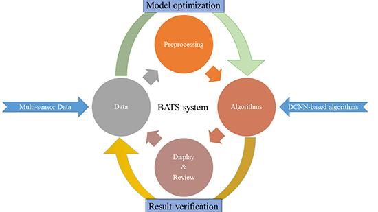
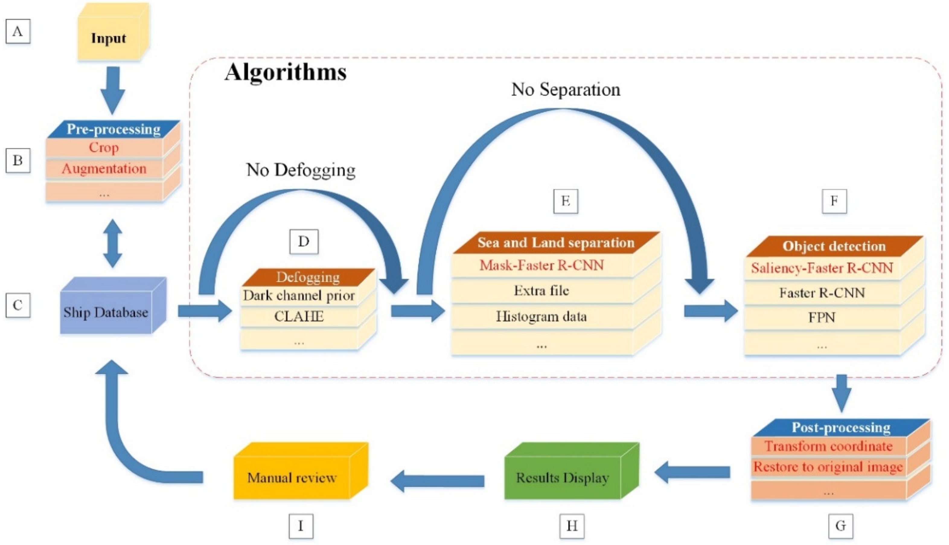
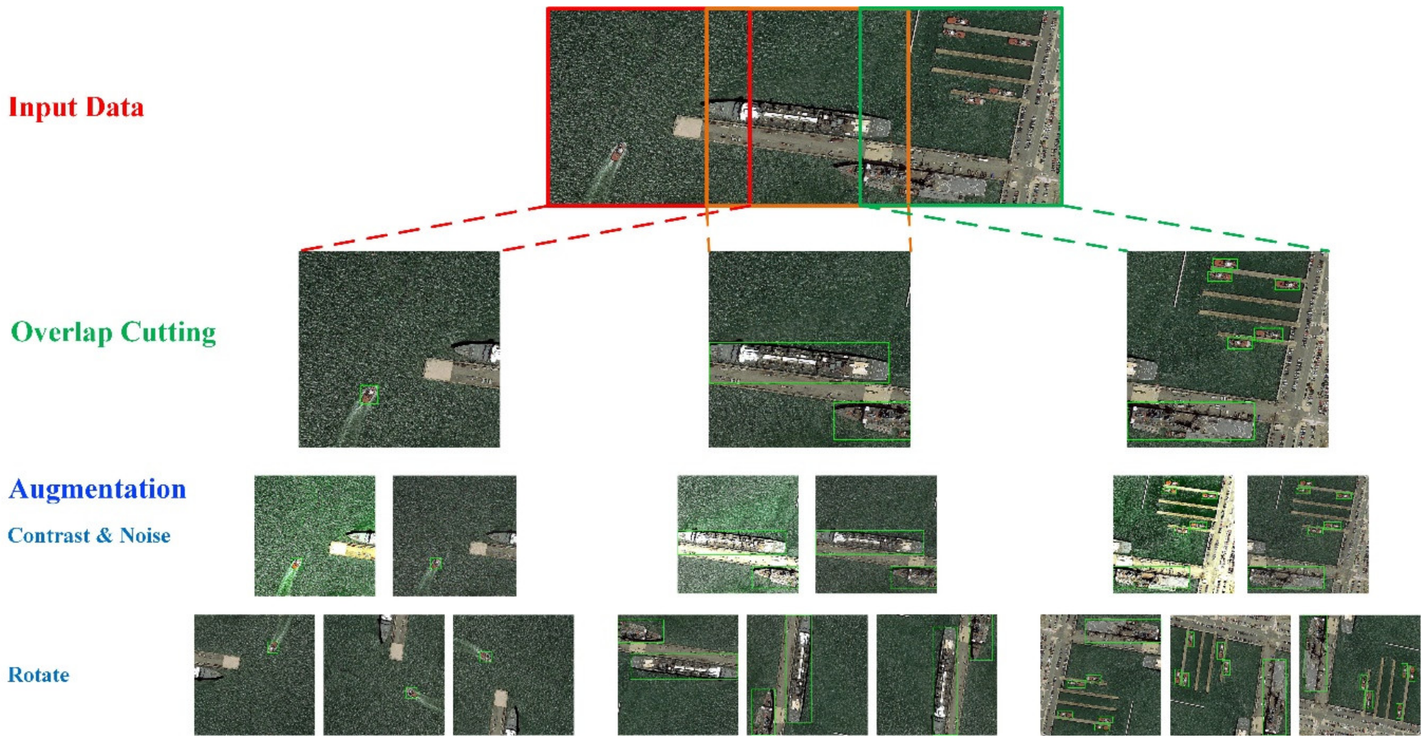
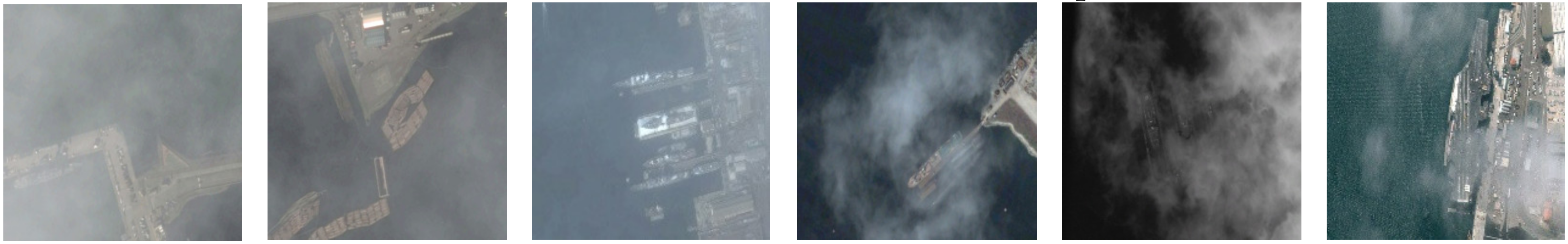
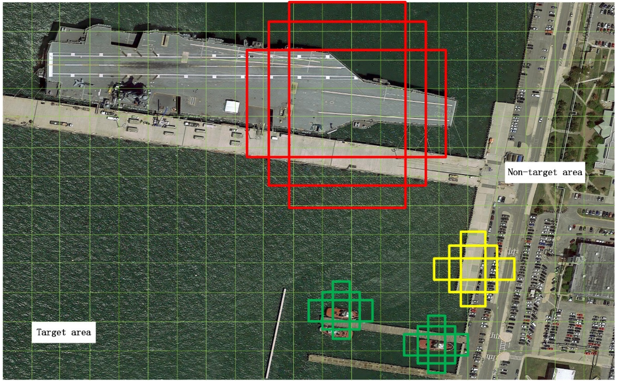
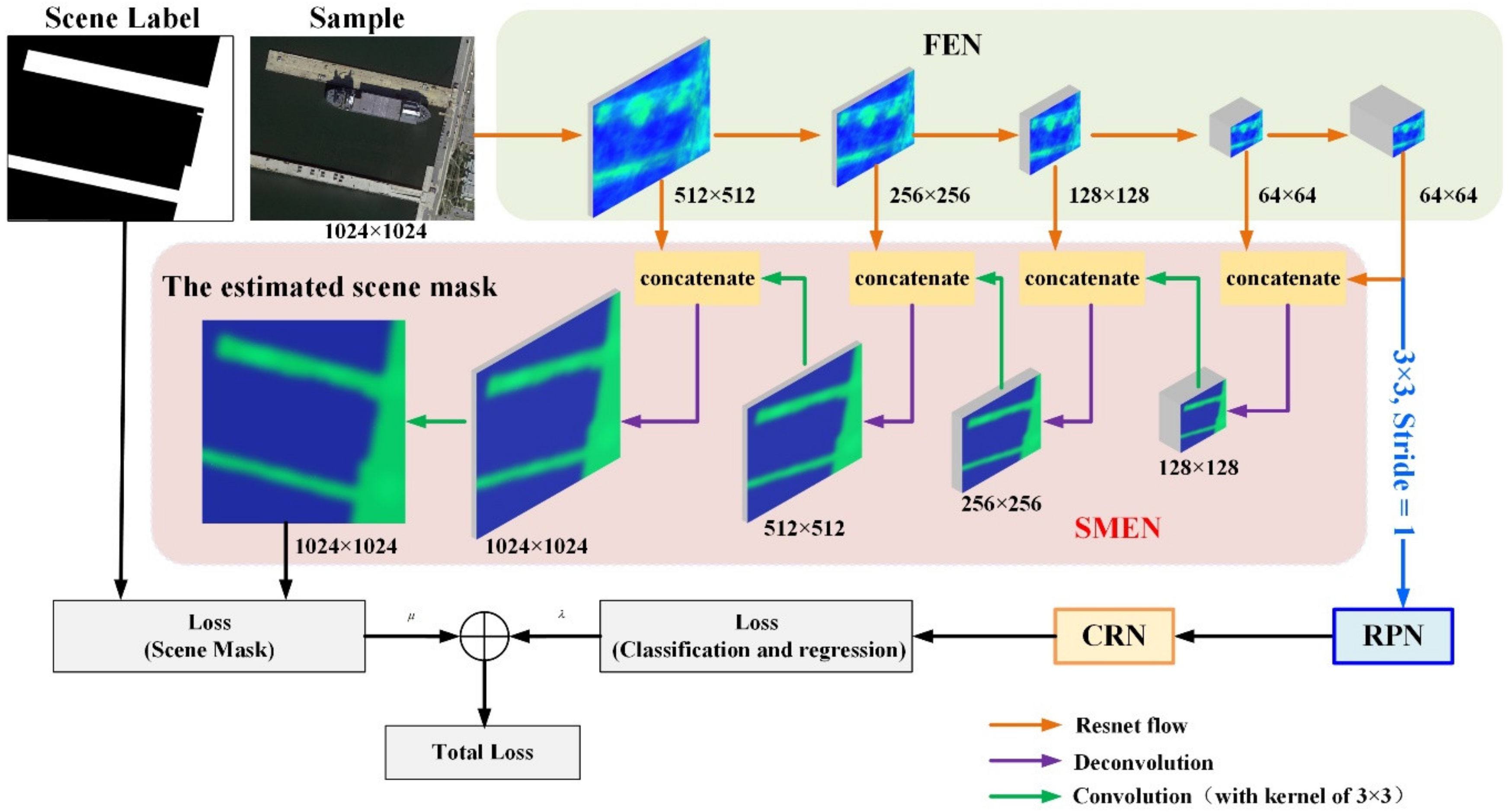
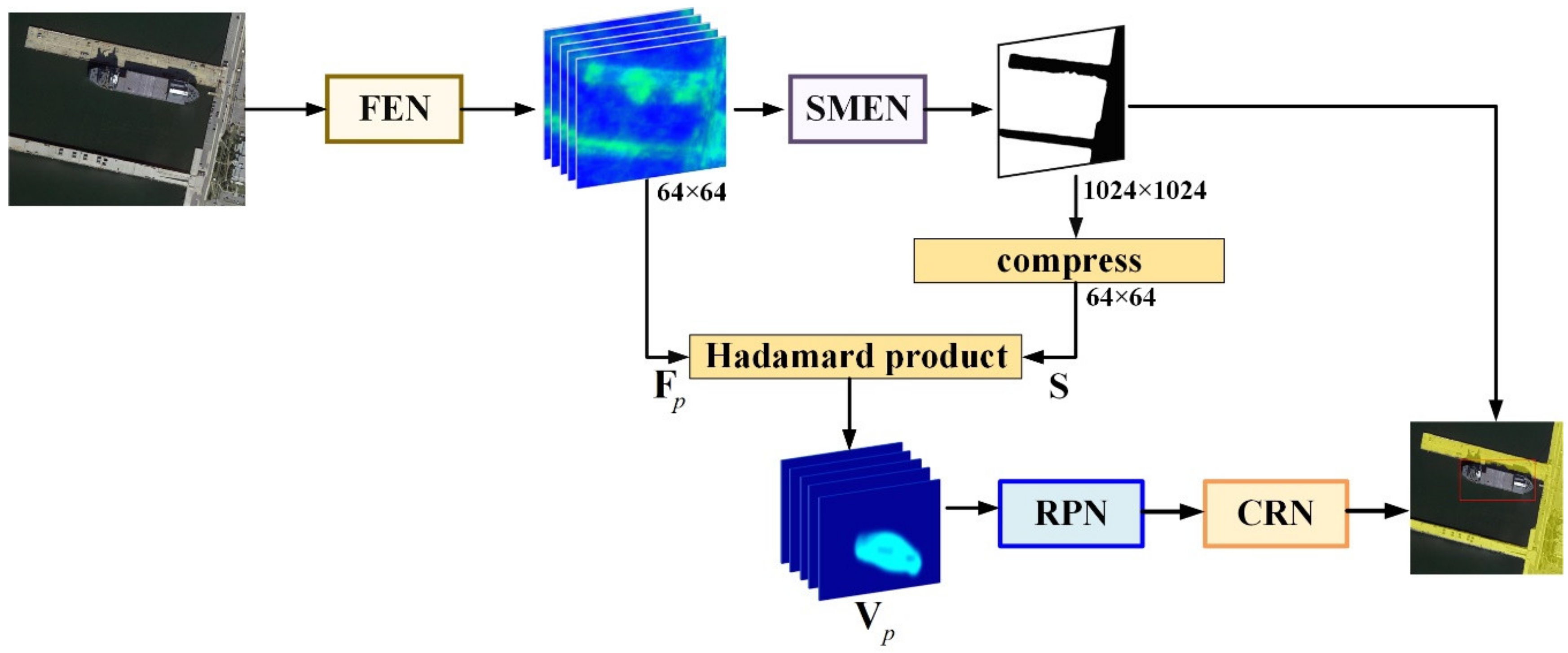
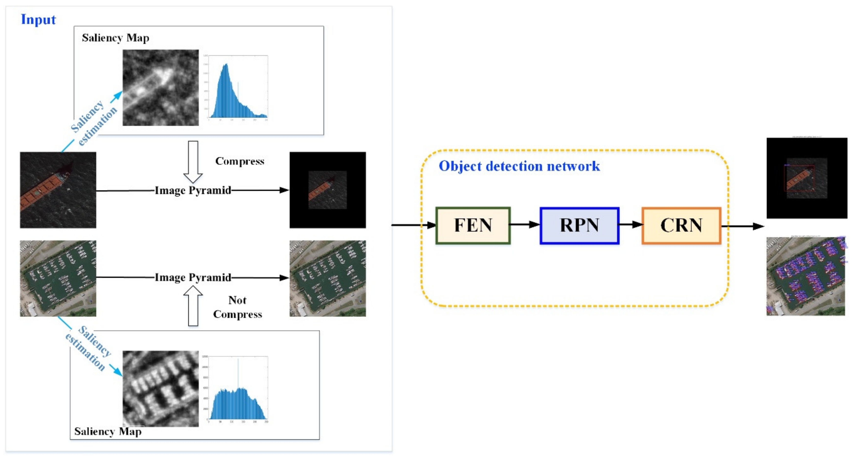
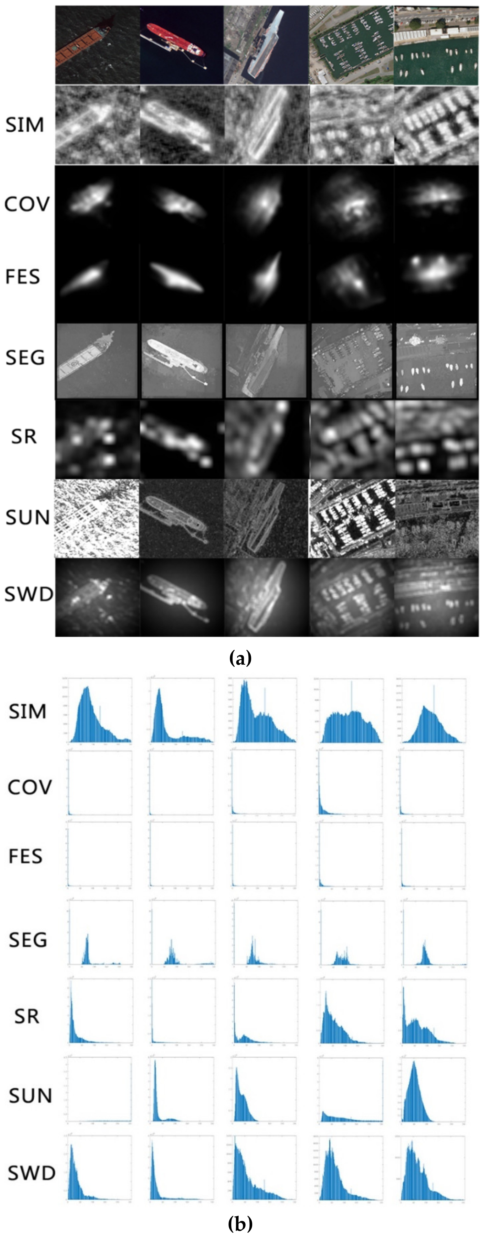
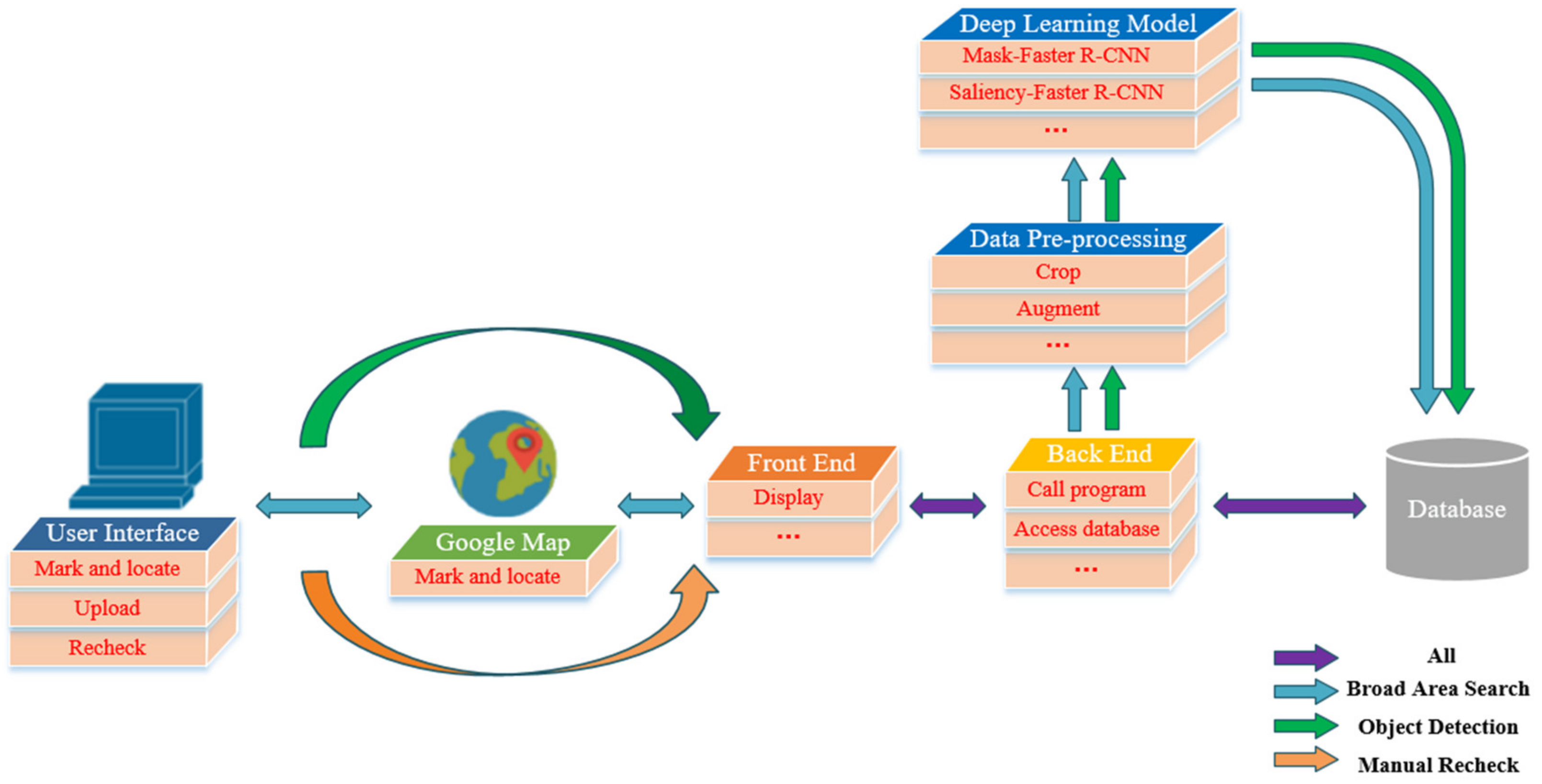
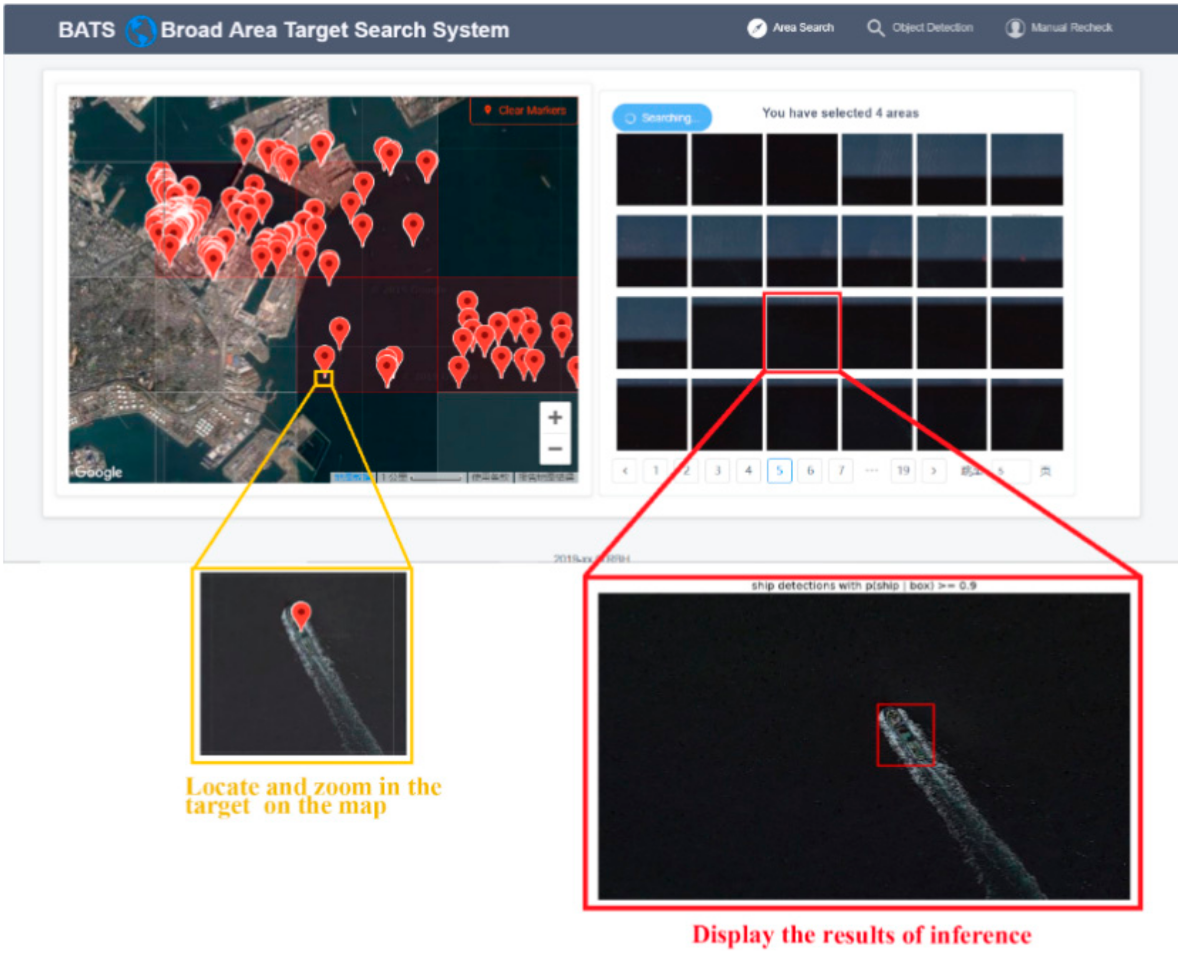
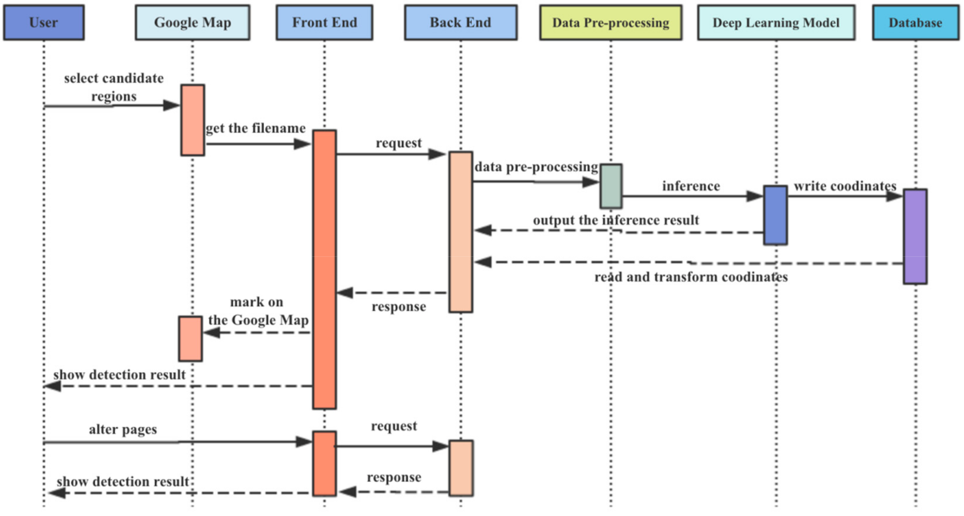
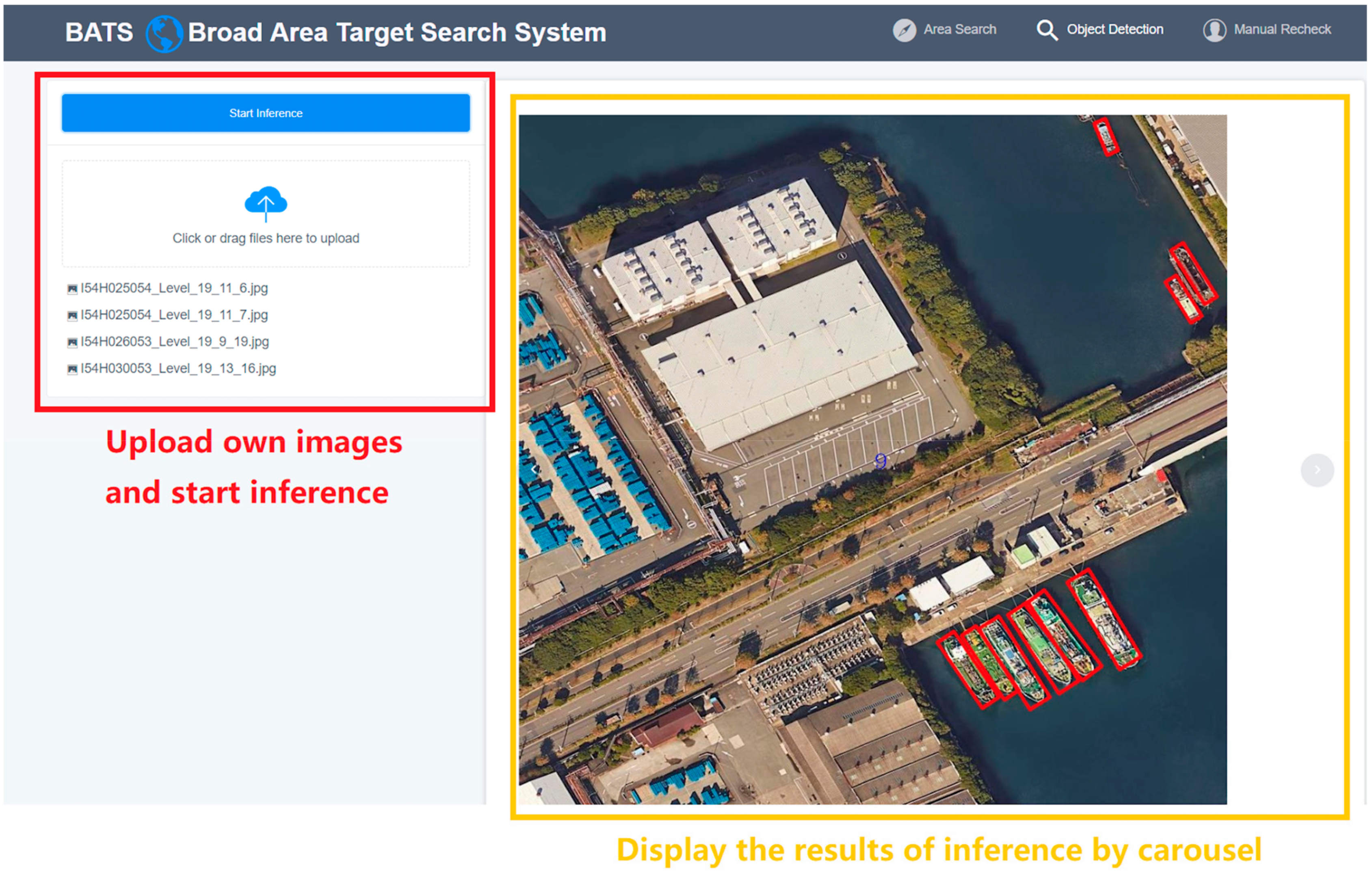
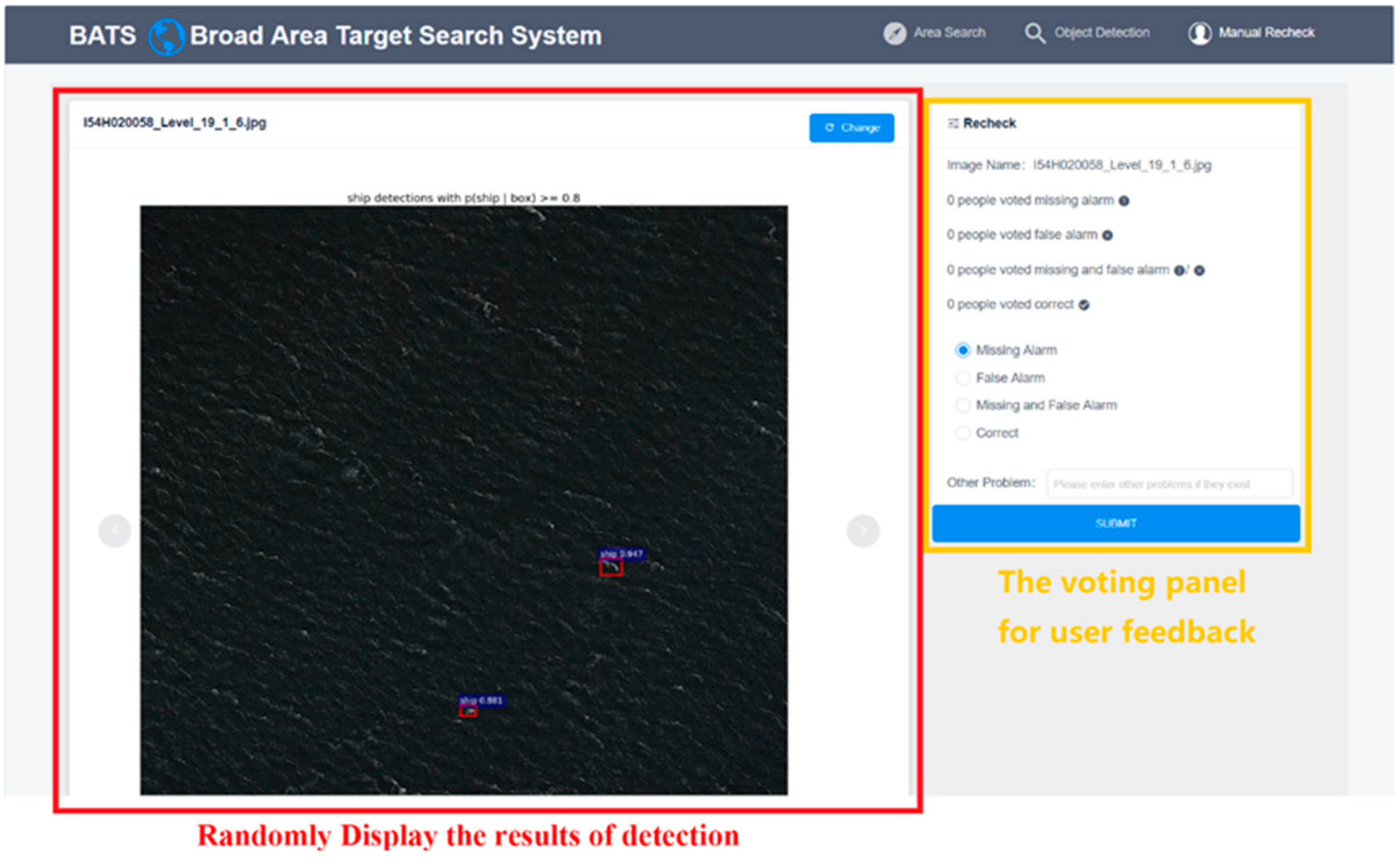
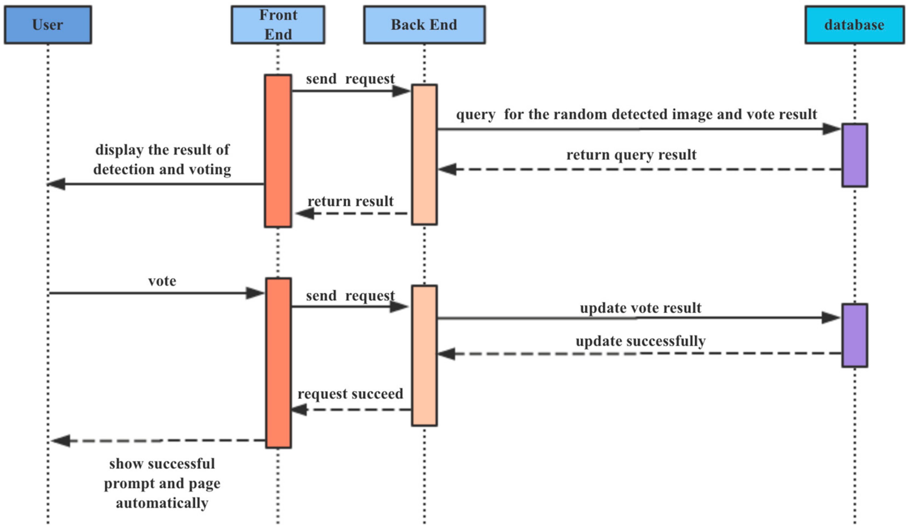
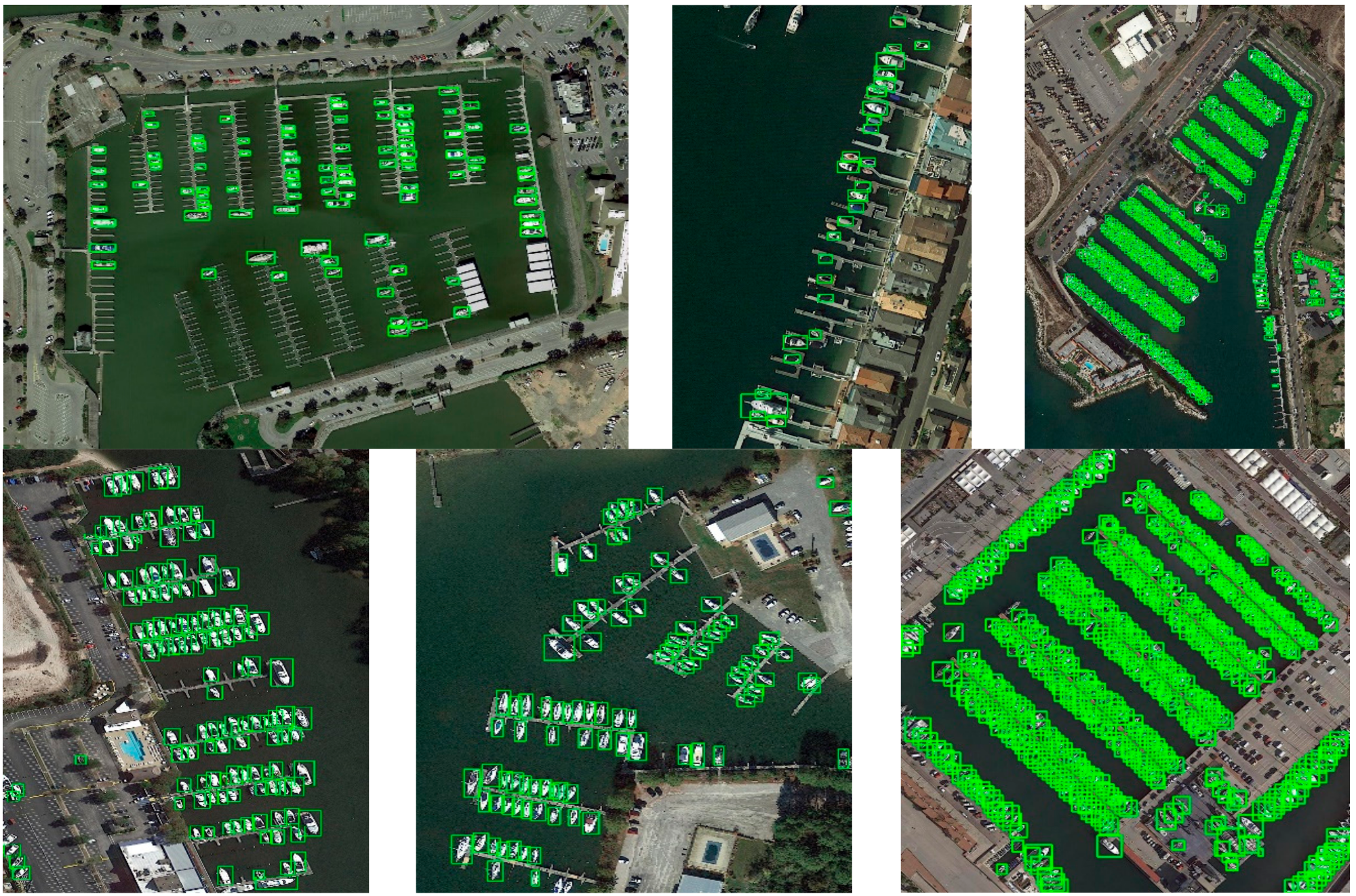
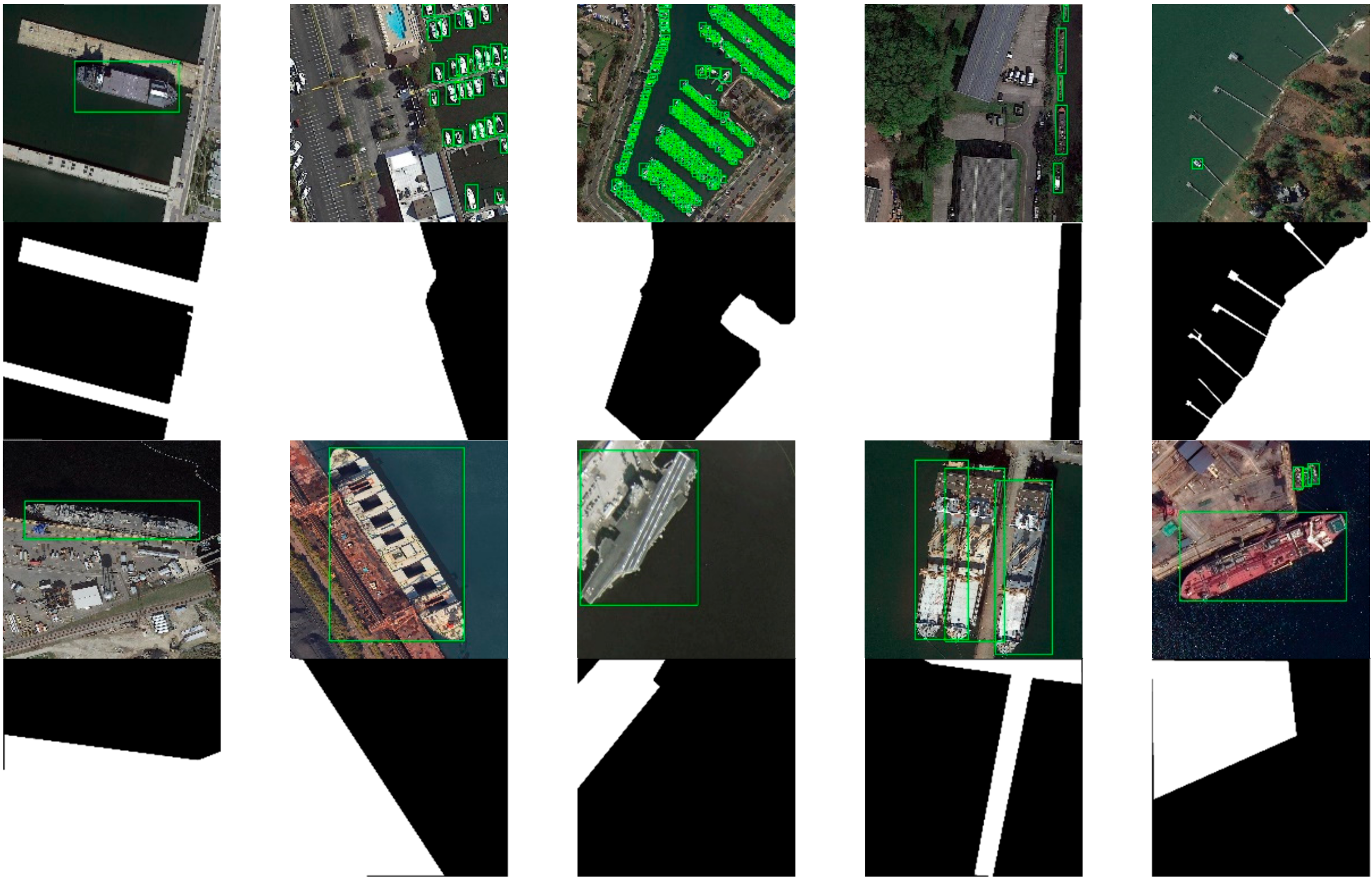
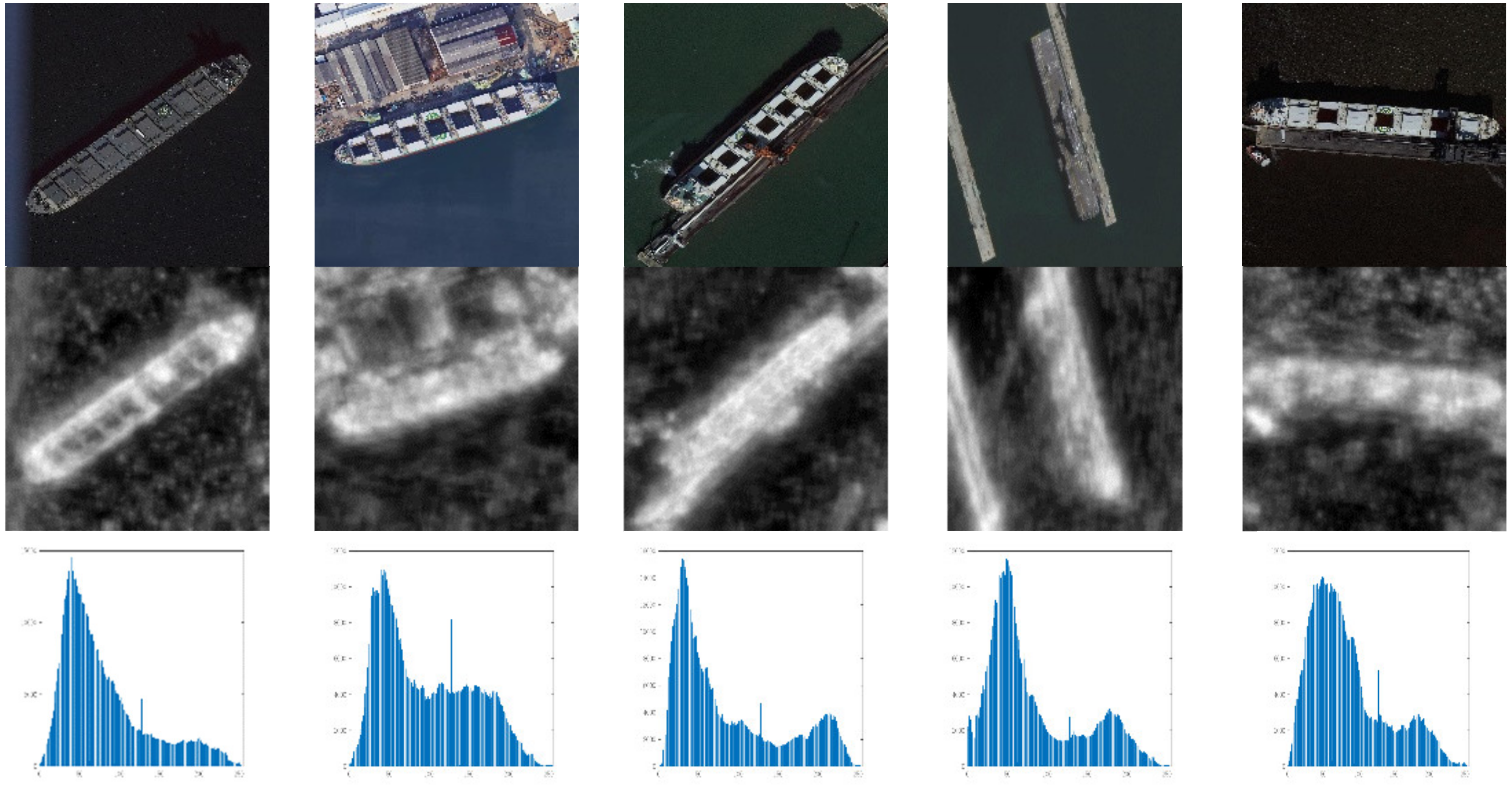
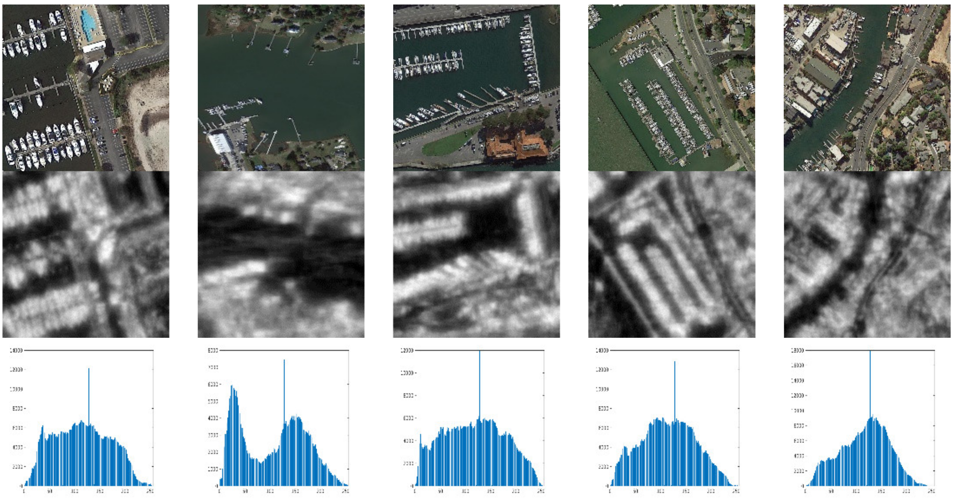
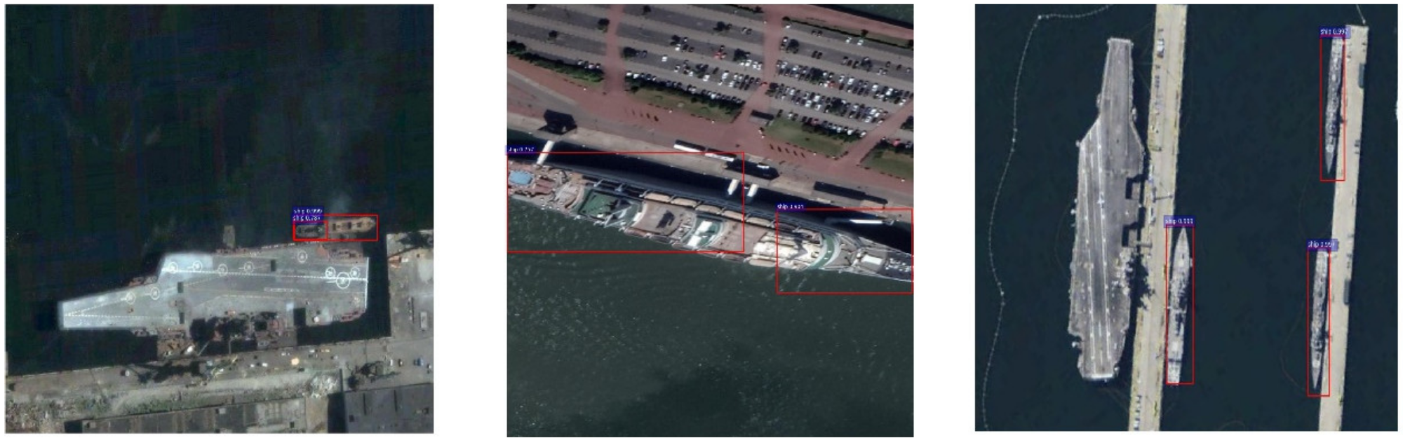
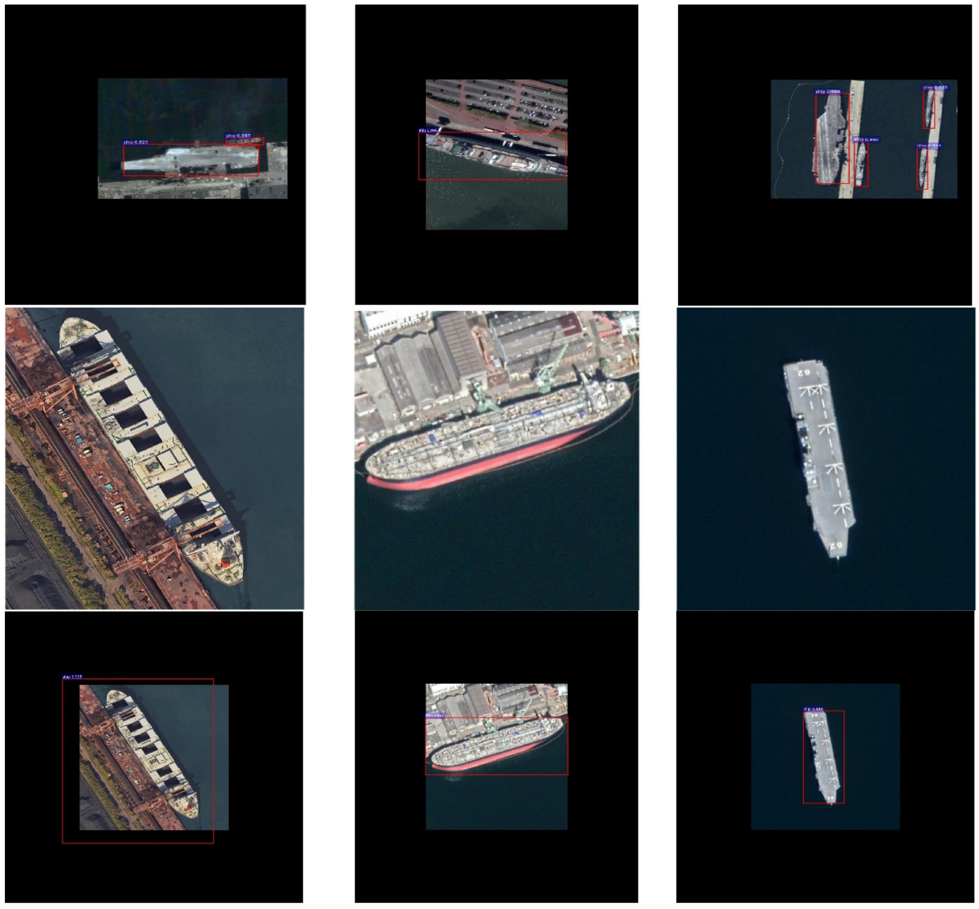
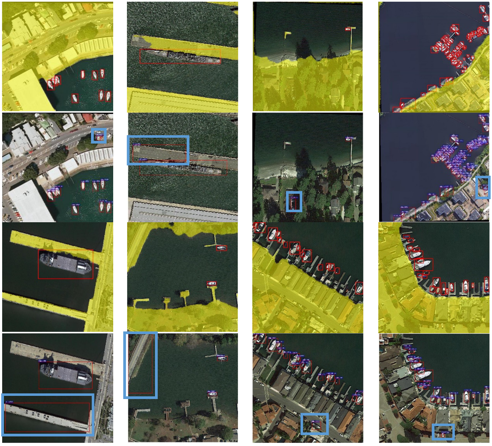
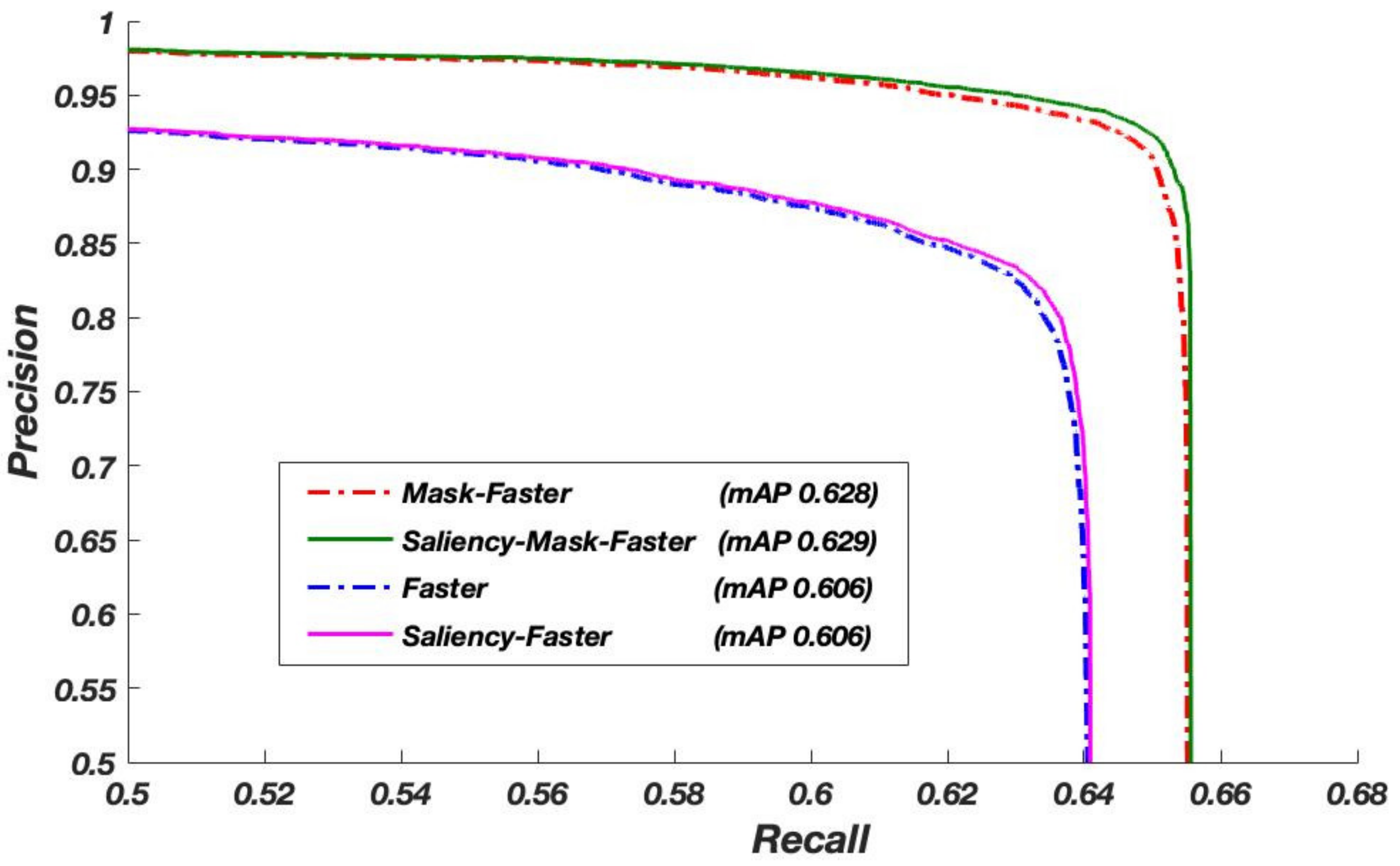
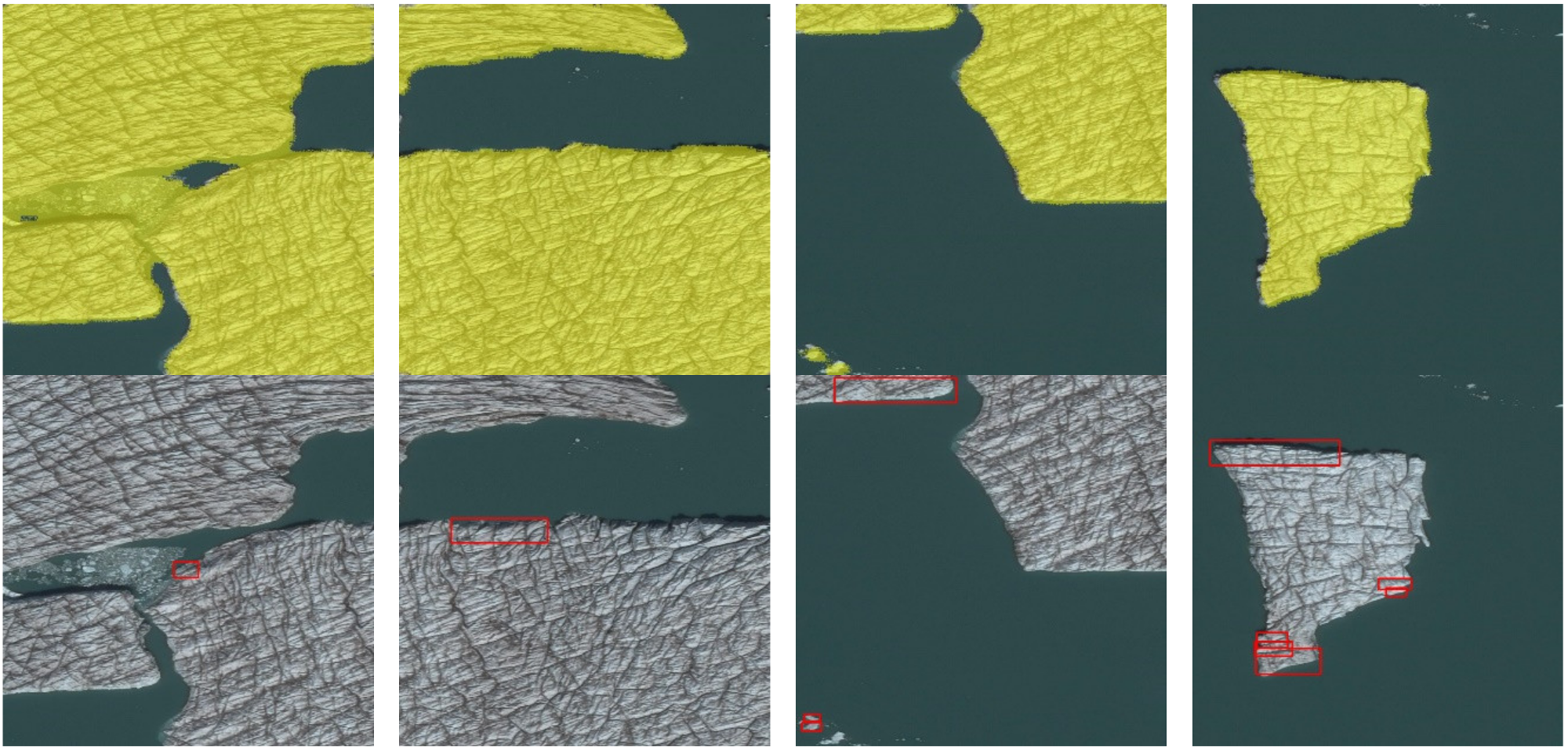
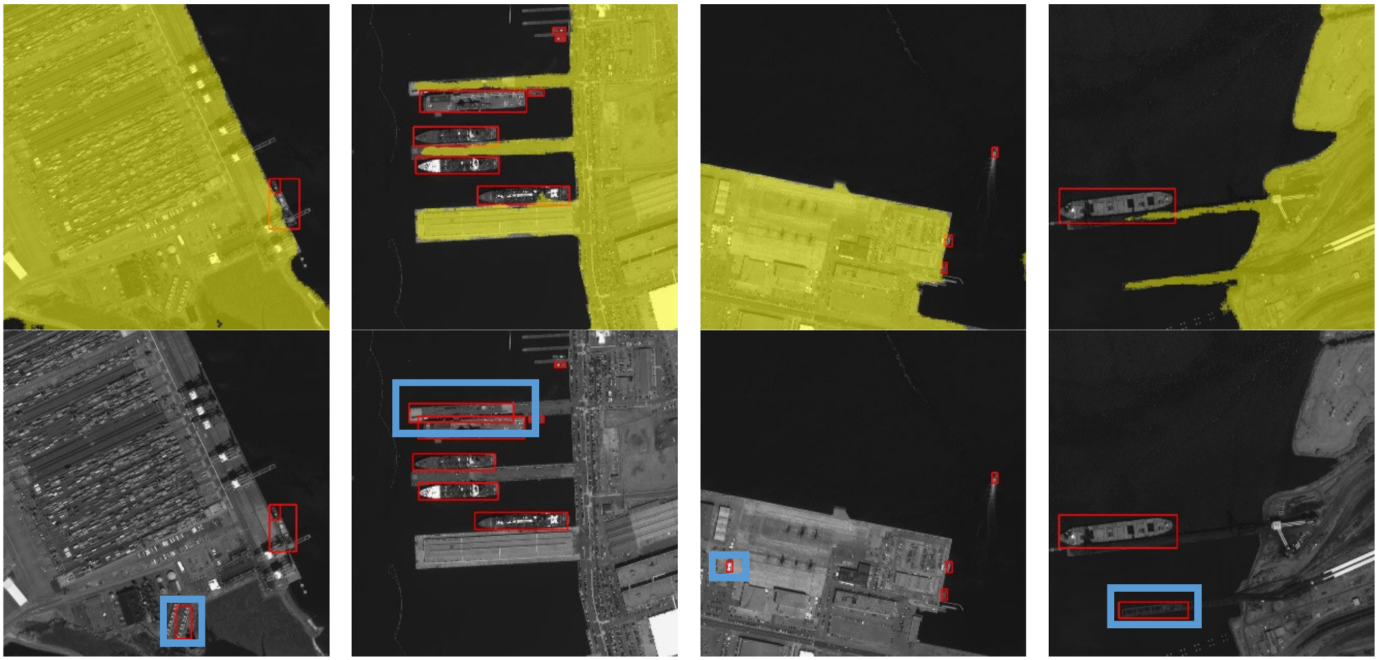
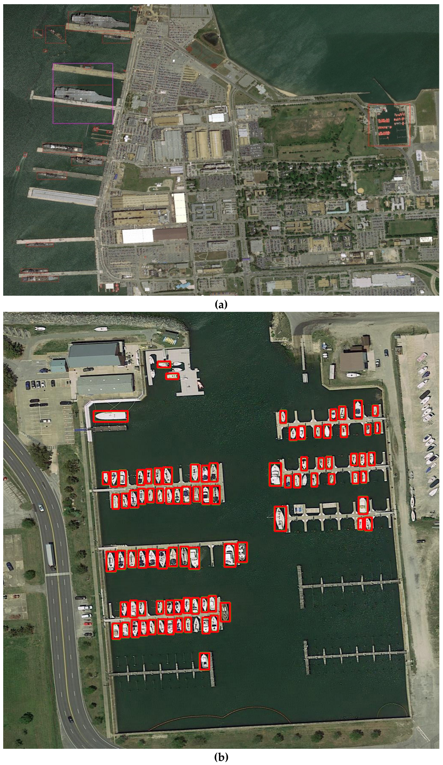
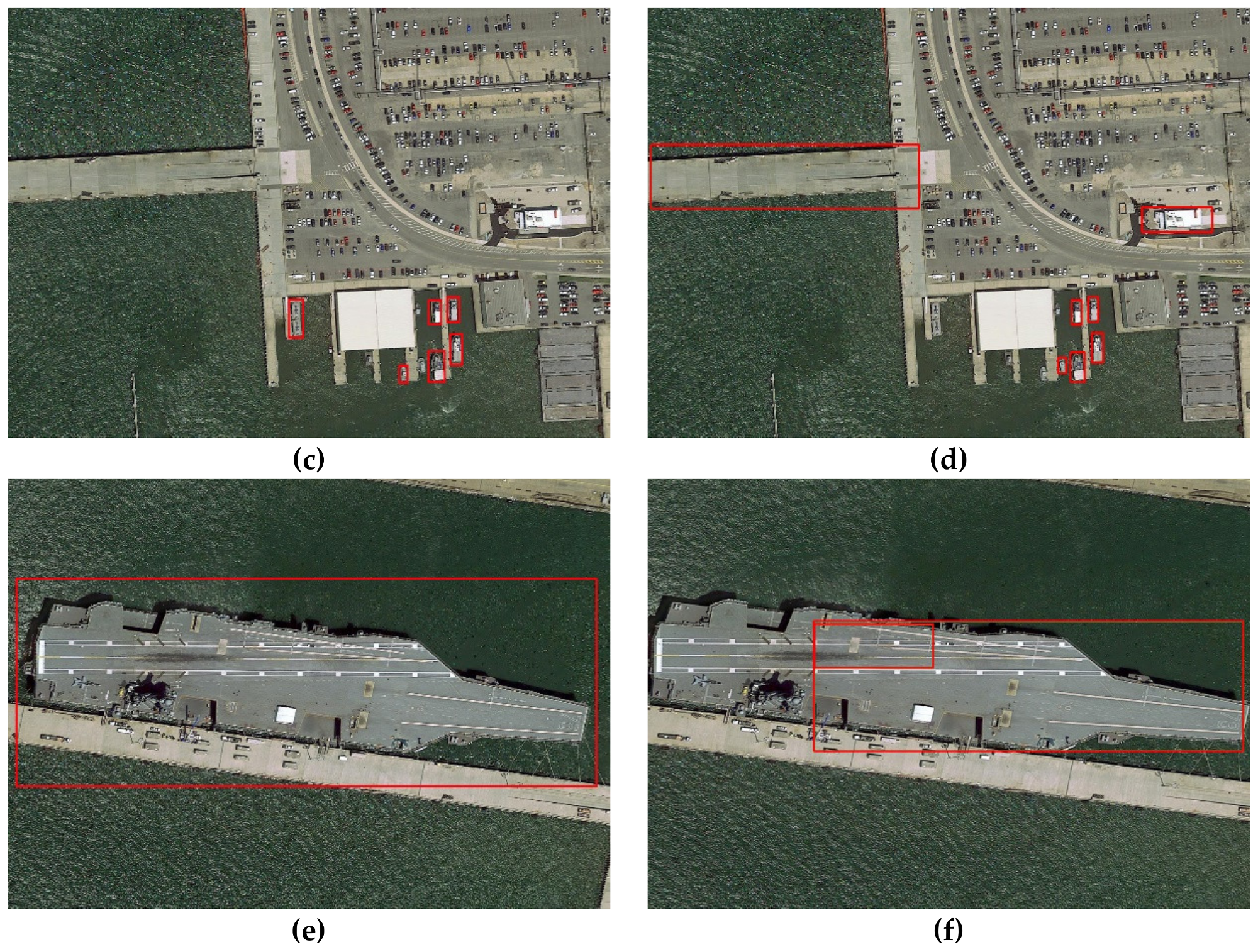
Table 1.
Configuration of the Resnet-101 in object detection network.
| Block | Output Size | Layers | Layer parameter |
|---|---|---|---|
| Part1 (FEN) | |||
| Conv1 | 512×512×64 | Convolution | 7×7, 64, stride = 2 |
| Pool1 | 256×256×64 | Max pooling | 3 × 3, stride = 2 |
| Block1 | 128×128×256 | Convolution group | ×3, stride = 2 |
| Block2 | 64×64×512 | Convolution group | ×4, stride = 2 |
| Block3 | 64×64×1024 | Convolution group | ×23, stride = 1 |
| Part2 (used after ROI Pooling) | |||
| Block 4 | 7×7×2048 | Convolution group | ×3, stride = 2 |
| Pool2 | 7×7×2048 | Average pooling | 2×2, stride = 1 |
Table 2.
Configuration of the scene mask extraction network.
| Layers | Layer parameter | Output size |
|---|---|---|
| Deconv 1 | 3 × 3, 512, stride = 2 | 128 × 128 × 512 |
| Conv 1 | 3 × 3, 512, stride = 1 | 128 × 128 × 512 |
| Deconv 2 | 3 × 3, 256, stride = 2 | 256 × 256 × 256 |
| Conv 2 | 3 × 3, 256, stride = 1 | 256 × 256 × 256 |
| Deconv 3 | 3 × 3, 128, stride = 2 | 512 × 512 × 128 |
| Conv 3 | 3 × 3, 128, stride = 1 | 512 × 512 × 128 |
| Deconv 4 | 3 × 3, 64, stride = 2 | 1024 × 1024 × 64 |
| Conv 4 | 3 × 3, 2, stride = 1 | 1024 × 1024 × 2 |
| Softmax | 1024 × 1024 × 2 |
Table 3.
Comparison of the Saliency-Faster R-CNN and Faster R-CNN.
| Method | AP | APL | NCR |
|---|---|---|---|
| Faster R-CNN | 0.606 | 0.664 | N/A |
| Saliency-Faster R-CNN | 0.606 | 0.727 | 0.105 (16/152) |
Table 4.
Comparison of the Mask-Faster R-CNN and Faster R-CNN.
| Method | AP | False Rate | mIOU |
|---|---|---|---|
| Faster R-CNN | 0.606 | 0.686 | N/A 0.877 |
| Mask-Faster R-CNN | 0.628 | 0.397 |
Table 5.
The comparison of time consumption.
| Baseline (Faster R-CNN) | Mask | Saliency | AP | Time (sec/image) |
|---|---|---|---|---|
| √ | 0.606 | 0.173 | ||
| √ | √ | 0.606 | 2.181 | |
| √ | √ | 0.628 | 0.231 | |
| √ | √ | √ | 0.629 | 2.233 |
Table 6.
The results of the system efficiency test.
| Size (MBytes) | Image pixels | Upload (sec/image) | Pre-processing (sec/image) | Post-processing (sec/image) | Num of Images |
|---|---|---|---|---|---|
| 1440.4 | 8576 × 5176 | 1.55 | 0.155 | 0.232 | 77 |
| 99.1 | 5896 × 5328 | 1.12 | 0.098 | 0.235 | 49 |
| 540.1 | 17152 × 10352 | 5.34 | 1.068 | 0.241 | 273 |
© 2019 by the authors. Licensee MDPI, Basel, Switzerland. This article is an open access article distributed under the terms and conditions of the Creative Commons Attribution (CC BY) license (http://creativecommons.org/licenses/by/4.0/).
Share and Cite
MDPI and ACS Style
You, Y.; Li, Z.; Ran, B.; Cao, J.; Lv, S.; Liu, F. Broad Area Target Search System for Ship Detection via Deep Convolutional Neural Network. Remote Sens. 2019, 11, 1965. https://doi.org/10.3390/rs11171965
AMA Style
You Y, Li Z, Ran B, Cao J, Lv S, Liu F. Broad Area Target Search System for Ship Detection via Deep Convolutional Neural Network. Remote Sensing. 2019; 11(17):1965. https://doi.org/10.3390/rs11171965
Chicago/Turabian StyleYou, Yanan, Zezhong Li, Bohao Ran, Jingyi Cao, Sudi Lv, and Fang Liu. 2019. "Broad Area Target Search System for Ship Detection via Deep Convolutional Neural Network" Remote Sensing 11, no. 17: 1965. https://doi.org/10.3390/rs11171965
Note that from the first issue of 2016, this journal uses article numbers instead of page numbers. See further details here.