Article

Stepwise Disaggregation of SMAP Soil Moisture at 100 m Resolution Using Landsat-7/8 Data and a Varying Intermediate Resolution

1
Centre d’Etudes Spatiales de la BIOsphère (CESBIO, Université de Toulouse (CNES/CNRS/INRA,IRD/UPS), 31013 Toulouse, France
2
Faculty of Sciences and Techniques, Cadi Ayyad University, Marrakech 40000, Morocco
3
Center for Remote Sensing Application (CRSA), University Mohammed VI Polytechnic (UM6P), Benguerir 43150, Morocco
4
isardSAT S.L, Parc Tecnologic Barcelona Activa, 08042 Barcelona, Spain
*
Author to whom correspondence should be addressed.
Remote Sens. 2019, 11(16), 1863; https://doi.org/10.3390/rs11161863
Submission received: 25 June 2019 / Revised: 29 July 2019 / Accepted: 4 August 2019 / Published: 9 August 2019
(This article belongs to the Special Issue Remote Sensing of Regional Soil Moisture)

Abstract

:
Global soil moisture (SM) products are currently available from passive microwave sensors at typically 40 km spatial resolution. Although recent efforts have been made to produce 1 km resolution data from the disaggregation of coarse scale observations, the targeted resolution of available SM data is still far from the requirements of fine-scale hydrological and agricultural studies. To fill the gap, a new disaggregation scheme of Soil Moisture Active and Passive (SMAP) data is proposed at 100 m resolution by using the disaggregation based on physical and theoretical scale change (DISPATCH) algorithm. The main objectives of this paper is (i) to implement DISPATCH algorithm at 100 m resolution using SMAP SM and Landsat land surface temperature and vegetation index data and (ii) to investigate the usefulness of an intermediate spatial resolution (ISR) between the SMAP 36 km resolution and the targeted 100 m resolution. The sequential disaggregation approach from 36 km to ISR (ranging from 1 km to 30 km) and from ISR to 100 m resolution is evaluated over 22 irrigated field crops in central Morocco using in-situ SM measurements collected from January to May 2016. The lowest root mean square difference (RMSD) between the 100 m resolution disaggregated and in-situ SM is obtained when the ISR is around 10 km. Therefore, the two-step disaggregation is more efficient than the direct disaggregation from SMAP to 100 m resolution. Moreover, we propose a moving average window algorithm to increase the accuracy in the 100 m resolution SM as well as to reduce the low-resolution boxy artifacts on disaggregated images. The correlation coefficient between 100 m resolution disaggregated and in situ SM ranges between 0.5–0.9 for four out of the six extensive sampling dates. This methodology relies solely on remote sensing data and can be easily implemented to monitor SM at a high spatial resolution over irrigated regions.

1. Introduction

Knowledge of soil moisture provides key information about the coupling between the land surface and atmosphere. By controlling the partitioning of water inputs (precipitation, irrigation) into evaporation, infiltration, and runoff, the soil water content is related to the crop water consumption [1], hydrological fluxes [2], weather predictions [3] and climate projections [4].
L-band (1.4 GHz) microwave radiometry is currently the most adapted remote sensing technique for the estimation of near-surface soil moisture (SM) from space [5,6,7,8,9,10]. Microwave observations at L-band, as compared to higher microwave frequencies, are more sensitive to SM and less sensitive to the soil surface roughness and vegetation optical depth [11]. In this context, European Space Agency (ESA) and National Aeronautics and Space Administration (NASA) have launched the SMOS [6,12] and SMAP [5] satellites in 2009 and 2014, respectively. Both satellites embark an L-band radiometer to retrieve the 3–5 cm SM with a repeat cycle of less than 3 days globally. The spatial resolution of both radiometers is approximately 40 km [5,6].
Despite the high radiometric accuracy achieved by L-band radiometers, the data provided globally have a low spatial resolution, which makes the validation of remote sensing products difficult and limits their application to large scale studies only [13]. For hydro-agriculture purposes, there is a crucial need for SM data at a higher spatial resolution [14,15]. Consequently, disaggregation techniques have been proposed to improve the spatial resolution of the SM data available at a high temporal frequency [16,17,18,19,20,21,22]. Existing downscaling methods for SM can be classified into three major groups (1) satellite-based methods; (2) methods using Geo-information data and (3) model-based methods [23,24]. The satellite methods combine the use of radar and optical data to coarse scale microwave radiometry [24]. Among optical-based methods, many studies have used as fine-scale information the fractional vegetation cover and land surface temperature (LST) derived from high-resolution (1 km to 100 m) optical/thermal sensors. The general idea of these methods is to relate LST to SM via the evapotranspiration process [20,25].
Relying on this principle, the disaggregation based on physical and theoretical scale change (DISPATCH) method [26,27] estimates the soil evaporative efficiency (SEE defined as the ratio of actual to potential soil evaporation), and implements a downscaling relationship that links the disaggregated SM to the low-resolution (LR) observation and the high-resolution (HR) SEE. The optical-derived SEE is expressed as a linear function of the retrieved soil temperature [28] and the minimum and maximum soil temperatures observed at HR within the LR pixel [26], according to the so-called contextual approach [29]. Based on the DISPATCH algorithm, the CATDS Level-4 Disaggregation (C4DIS) processor [30] was implemented at the Centre Aval de Traitement des Donnees SMOS (CATDS) as a level 4 product. C4DIS produces 1 km resolution SM data at the quasi-global scale from SMOS level 3 and Moderate resolution Imaging Spectroradiometer (MODIS) data.
The 1 km resolution SM disaggregated from SMOS produts are currently used in a range of disciplines including root-zone soil moisture monitoring [31], detecting irrigated areas at the perimeter scale [32,33], retrieving soil properties from space [34], preventing the spread of desert locust swarms [35], evapotranspiration monitoring over rainfed areas [36], flood forecasting over large basins [37], estimating crop yield [38], and the methods to produce them are continuously evolving and maturing (Merlin et al. 2017). Note that few studies have applied the DISPATCH method to SMAP SM using MODIS data [39]. However, the 1 km resolution is often insufficient for many other fine-scale applications and areas where the surface is highly heterogeneous (e.g., [1]). SM data at the sub-kilometric (typically hectometric) resolution are especially required in agriculture for early crop detection, irrigation scheduling, water stress and yield monitoring [40] and in fine-scale hydrological studies for flood risk prevention, drought monitoring and groundwater level assessment [41], among other potential applications.
In fact, there is still no routine application of DISPATCH to Landsat data, which yet would be useful to increase the spatial resolution of available SM products up to 100 m [27,42]. One difficulty is that Landsat data do not provide global coverage at the daily scale (like MODIS data) so that a sequential approach is needed to “delineate” the 1 km resolution disaggregated SMAP data over each Landsat scene separately before DISPATCH can be implemented at 100 m resolution. Another difficulty is the contextual nature of DISPATCH, which relies on the extreme wet and dry conditions present within the LR pixel to calibrate the SEE model. Especially, the accuracy in temperature endmembers is expected to vary with the spatial extent over which DISPATCH is applied. A third difficulty is the presence of boxy artifacts visible at LR when combining multi-source/multi-resolution remote sensing data within a disaggregation methodology. Boxy artifacts are common problems with downscaling methods [26,27,43].
In this context, this paper presents a new methodology to disaggregate optimally the 36 km resolution SMAP SM to 100 m resolution using Landsat data. The main objective is to assess the usefulness of an optimal intermediate spatial resolution (ISR) between the SMAP and Landsat resolutions. In practice, the 1 km resolution SM disaggregated from SMAP data using MODIS data (similar to C4DIS product for SMAP) is aggregated at ISR ranging from 1 km to 30 km, and DISPATCH is applied to ISR SM. The novelty of this paper thus lies in: (1) the application of DISPATCH to SMAP data at 100 m resolution, (2) the use of an ISR between SMAP and Landsat resolutions and (3) the removal of boxy artifacts on the 100 m resolution disaggregated images using a new technique.
Herein, the stepwise disaggregation approach is tested over an experimental area in central Morocco, comprised of 22 irrigated field crops over which the 0–5 cm SM has been monitored during the 2015–2016 season.

2. Materials and Methods
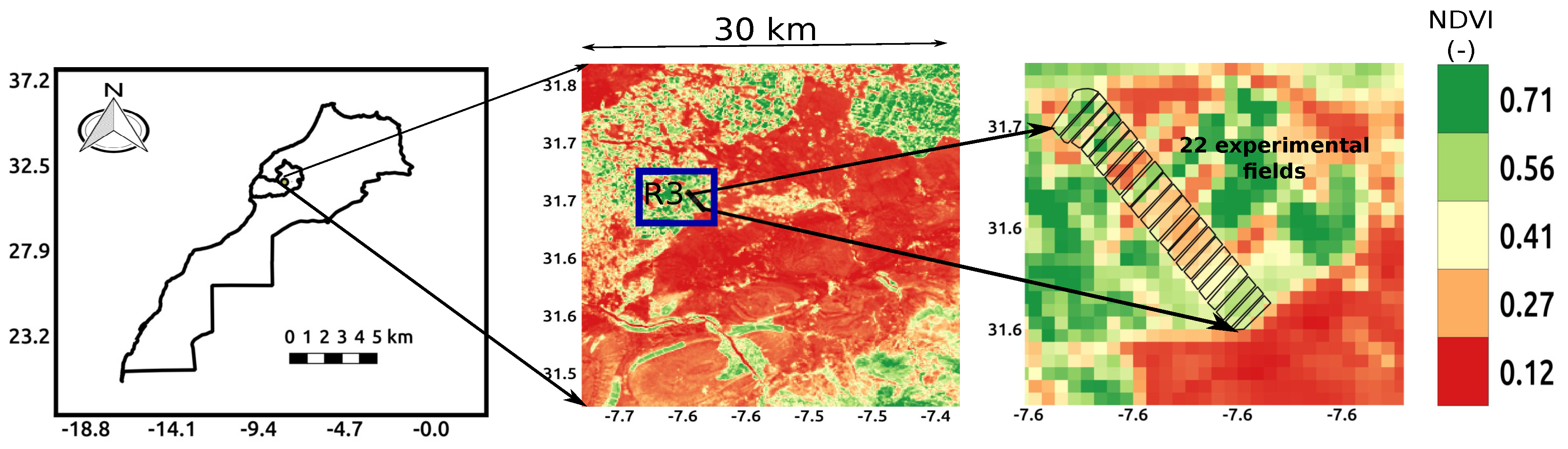
2.1. Study Area

The study focuses on a 30 km by 30 km area of the R3 irrigated zone (31.70N, 7.35W) located 40 km east of Marrakesh city in the Haouz plain, central Morocco (see Figure 1). To assess the performance of DISPATCH at the 100 m resolution, a set of 22 irrigated wheat fields, covering 3–4 ha each (Figure 1), were selected within a 1 km resolution MODIS pixel. SM sampling was undertaken on clear sky dates with almost simultaneous SMAP/MODIS/Landsat data over the 22 crop fields and repeated measurements were made along the agricultural season to cover all the phenological stages of wheat. Climate of the study area is mainly semi-arid with an annual average precipitation of 250 mm [44,45]. The soil texture in the R3 perimeter is mainly clayey. Flood irrigation is the most widely used method in this district. Wheat is generally sown in November-December and a mean total of 6 irrigations is applied to wheat crops from February till April, typically every 3 weeks. Harvesting is done in late May or early June [46,47].

2.2. In-Situ Data

The 0–5 cm SM was measured manually from January to May months during the 2015–2016 agricultural season. The sampling strategy was to use theta probes to collect 10 distinct measurements for each of the 22 crop fields [48]. In practice, as the 22 parcels were chosen to be aligned and contiguous, two transects along both sides of the crop fields were walked and 5 theta probes measurements were taken on each crop side, at least 5 m from the field border. Theta probe measurements were calibrated using the gravimetric method, based on soil samples collected on each sampling date. In this study, the field-scale SM corresponds to the mean 0–5 cm calibrated theta probe measurements as in Amazirh et al. [49]. Among the 7 available sampling dates, only 6 are used herein in order to satisfy the following criteria: SM measurements are available on a clear-sky Landsat overpass date, and the time difference between SMAP and Landsat overpasses is one day at maximum. The clear-sky dates with quasi-concurrent in-situ sampling and the satellite overpasses of SMAP, SMOS, MODIS and Landsat were on DOY 6, 14, 30, 38, 62 and 78. The remaining sampling dates are suitable for our study and help us identify the variability in SM along the growth of crops.

2.3. Remote Sensing Data

2.3.1. SMAP

SMAP was launched by NASA on 31 January 2015. SMAP is the first L-band mission combining both radar (active) and radiometer (passive) data to provide SM at a range of resolutions from 3 km (active) to 36 km (passive) with a revisit cycle of 2–3 days. But due to the failure of the SMAP radar, the SM produced from SMAP is currently provided on a ∼36 km and ∼9 km (by using a re-sampling technique) resolution grid. Note that a product combining SMAP and C-Band Sentinel-1 data has been recently provided by the mission [50]. SMAP has a near-polar sun-synchronous orbit at an altitude of 658 km with 6:00 a.m./p.m. local time descending/ascending overpass. SMAP works on multi-polarization with a fixed incidence angle at 40 degrees and a swath of ∼1000 km [5]. In this paper, the SMAP level-3 (product name SPL3SMP A/D, version 005, Colliander et al. [51]) is used. The product is provided in HDF format on the version 2 cylindrical EASE grid at 36 km resolution. Data can be downloaded from https://nsidc.org/data/SPL3SMP/versions/5.

2.3.2. MODIS

MODIS LST and NDVI data are used by the C4DIS processor [30] to provide the 1 km resolution SM from the disaggregation of SMAP level-3 SM data. LST is extracted from version 5 MOD11A1, Terra overpass (10:30 a.m.) on ascending node and MYD11A, Aqua overpass (1 p.m.) on descending node. For each (ascending or descending) SMAP overpass, there are 6 MODIS LST products taken as input to C4DIS (one day before, same day and one day after SMAP overpass for both Aqua and Terra platforms). NDVI is extracted from version 5 MOD13, only for Terra overpass with an interval of 16 days [19,52].

2.3.3. Landsat

Landsat-7 and Landsat-8 were launched by NASA in April 1999 and February 2013, respectively. The images were downloaded from the USGS website, which provides surface reflectance and thermal radiances data in different spectral bands. The revisit time of each sensor is 16 days and there is an 8-day lag between Landsat-7 and Landsat-8 so that the Landsat constellation potentially provides (in cloud-free conditions) optical/thermal data every 8 days globally. The Landsat-7/8 30 m resolution reflectance data are aggregated at 100 m resolution and used to derive the fractional vegetation cover. The Landsat NDVI is calculated as the ratio of the re-sampled near-infrared reflectance to re-sampled red reflectance difference divided by their sum, and the fractional vegetation ( f v ) is estimated as:
f v = N D V I H R N D V I s N D V I v N D V I s
where, N D V I H R represents the NDVI at high (100 m) resolution, N D V I s the NDVI at bare soil and N D V I v the NDVI at full cover vegetation. For this study, N D V I s and N D V I v are set to 0.1 and 0.9, respectively. Landsat-7 and Landsat-8 provide thermal infrared (TIR) data with a spatial resolution of 60 m and 100 m, respectively. LST is derived by using the single channel (SC) algorithm [53] from Landsat-7 band-6 and Landsat-8 band-7 as:
L S T = γ 1 ε φ 1 . L s e n + φ 2 + φ 3 + δ
where, ε is the surface emissitivity, ( γ , δ ) are parameters depending on the radiance and brightness temperature of the Landsat thermal band and φ 1 , φ 2 , φ 3 are atmospheric variables function of the atmospheric water vapor content ( ω ) and derived from radiative transfer simulations using the GAPRI database [54]. The ω variable is obtained from the MODIS product MOD05.

2.3.4. SRTM

SRTM (Shuttle Radar Topography Mission) 1 arc second global data are used to correct Landsat LST for topographic effects [27]. Although the study area is rather flat, the topographic correction is applied by default in DISPATCH. The 30 m resolution SRTM data are aggregated to 100 m resolution, consistent with the Landsat LST resolution.

2.4. DISPATCH

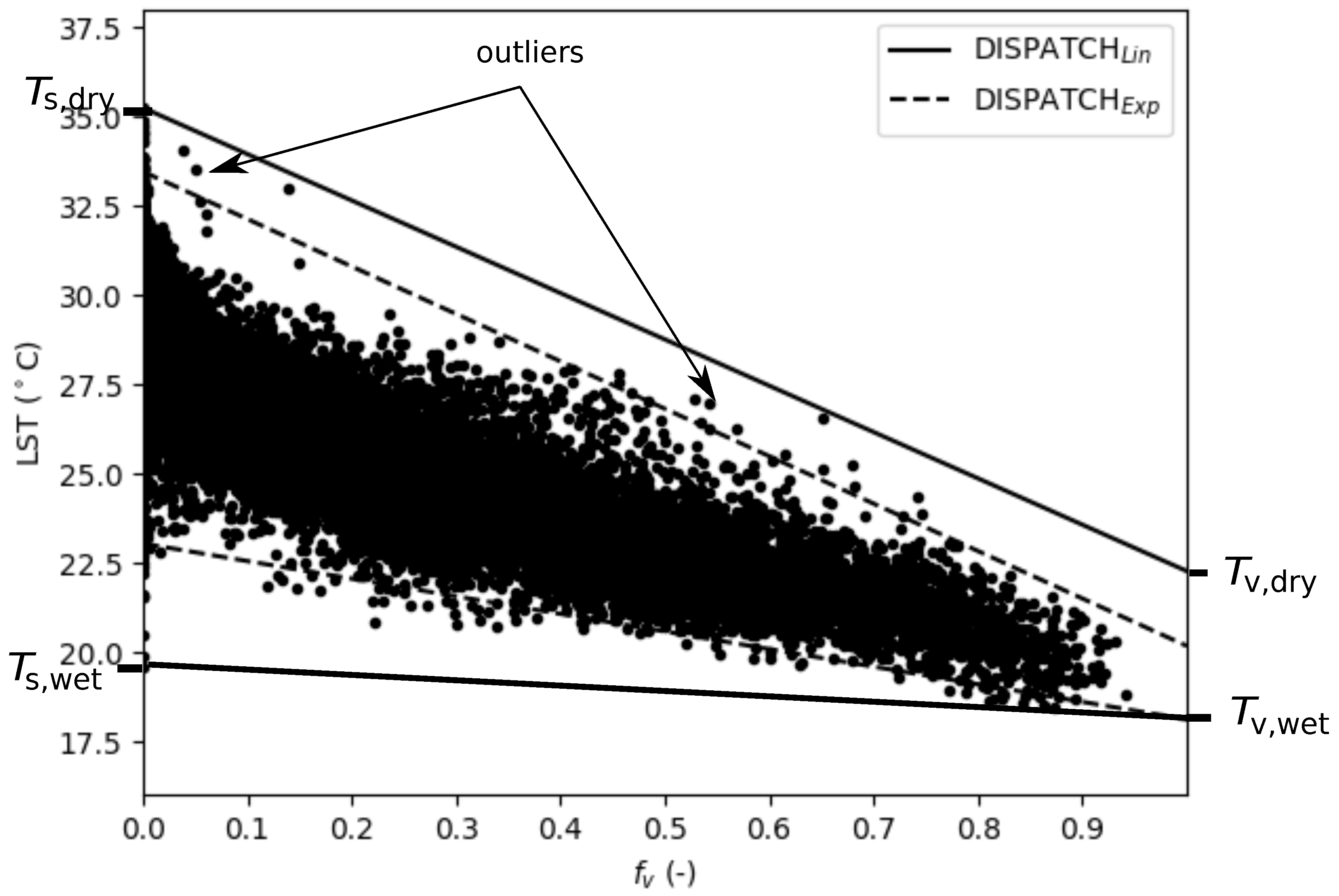
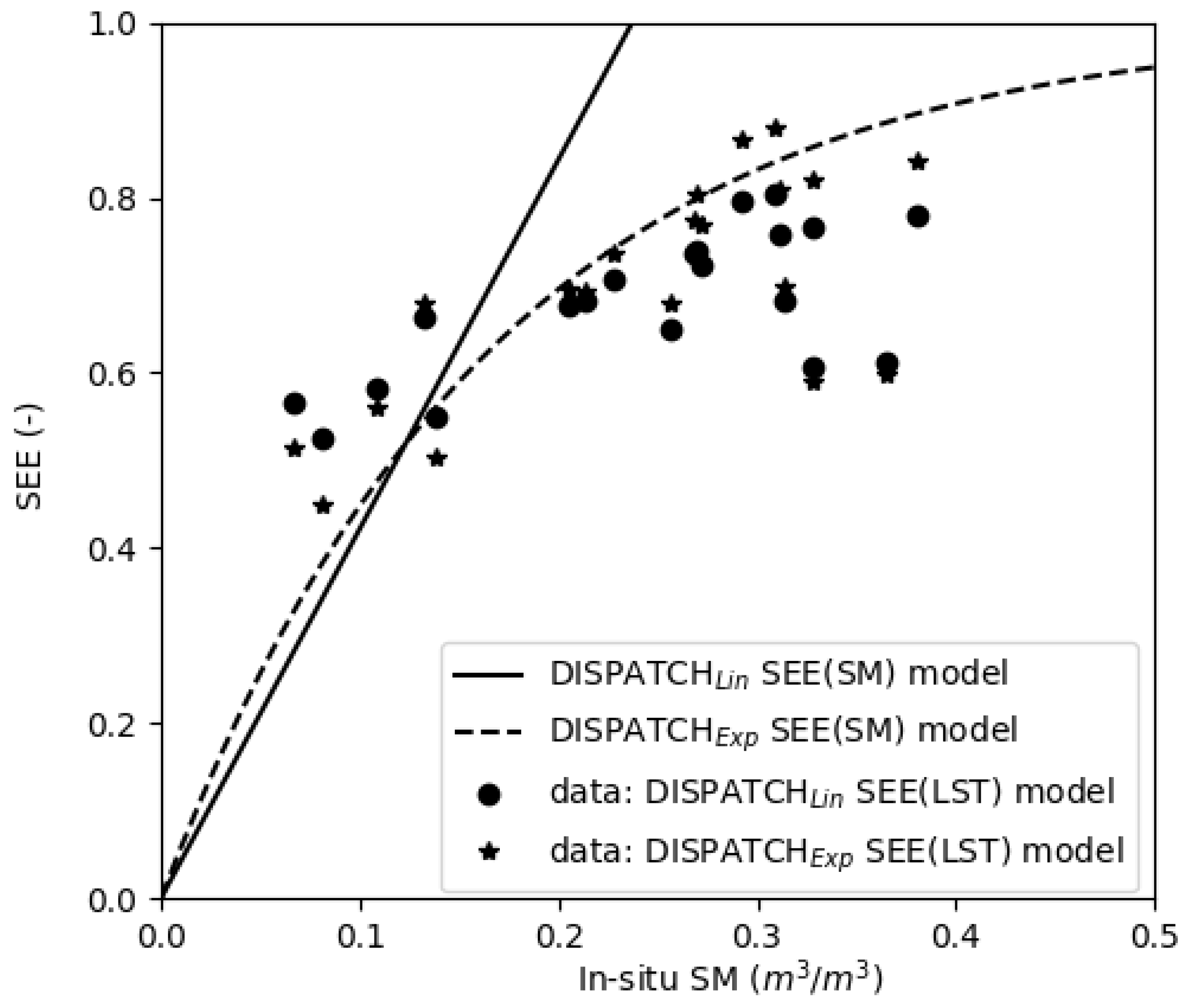
2.4.1. General Equations

The main equations of the DISPATCH method implemented at both 1 km and 100 m resolutions are reminded in this subsection. The SM downscaled at HR (refers to either 1 km or 100 m resolution) is written as:
S M H R = S M L R + δ S E E δ S M L R 1 S E E H R S E E L R
where, S M H R represents the disaggregated SM at HR, S M L R the SM at LR (refers to either SMAP or ISR resolution) derived from SMAP data or from their disaggregation to 1 km resolution, S E E H R the SEE at HR derived from MODIS or Landsat, S E E L R the HR SEE aggregated at LR, and δ S E E δ S M L R 1 the inverse of the partial derivative of the SEE(SM) model evaluated at LR. SEE is assumed to follow a linear relationship with the soil temperature [28] and is thus expressed as:
S E E H R = T s , d r y T s , H R T s , d r y T s , w e t
where T s is the soil surface temperature, T s , d r y and T s , w e t the soil temperature in fully dry (SEE = 0) and water-saturated (SEE = 1) conditions, respectively. Temperature endmembers T s , d r y and T s , w e t are calculated from a graph between LST and f v derived at HR from MODIS or Landsat data. The soil temperature is derived from a linear decomposition of LST into soil and vegetation temperature. The trapezoidal method [26,55] is used to estimate the vegetation temperature, and the soil temperature is expressed as the residual term:
T s , H R = T H R f v , H R T v , H R 1 f v , H R
where T H R represents the LST at HR, T v , H R the vegetation temperature at HR and f v , H R the fractional vegetation cover at HR.
The downscaling relationship of Equation (3) is hence based on two SEE models: SEE as a function of SM to estimate the first derivative at LR, and SEE as a function of LST (expressed in Equations (4) and (5)) to estimate the spatial variability of SM at HR.

2.4.2. DISPATCH at 1 km Resolution

Note that C4DIS is labeled as DISPATCH L i n (for linear SEE model) in this study to distinguish the methodologies applied at 1 km and 100 m resolution. The current version of C4DIS/DISPATCH L i n is based on the various studies that have been done in the past using 1 km resolution MODIS data (Merlin et al. 2013, 2012b, 2010, 2009, 2008). In DISPATCH L i n algorithm, the SEE(SM) model is linear:
S E E = S M S M p
where, S M p is a soil moisture parameter (in soil moisture unit), which depends on soil properties and atmospheric conditions. It is calibrated at the SMAP pixel scale at the satellite overpass time using LR SEE and SM estimates ( S M p = S M L R S E E L R ). In this case, the derivative in Equation (3) is simply S M p . The SEE(LST) model implemented in DISPATCH L i n is based on Equation (4) using the temperature endmembers calculated by the simplest extrapolation method within the LST- f v feature space: T s , d r y and T s , w e t are set to the maximum and minimum soil temperature within a given LR pixel.
This approach is implemented for C4DIS/DISPATCH L i n and has provided favorable results at 1 km resolution for arid and semi-arid areas [26,30].

2.4.3. DISPATCH at 100 m Resolution

When applying the DISPATCH methodology at 100 m resolution over extremely heterogeneous areas like irrigated perimeters, one expects two main differences with the 1 km case. First, the range of LST values should increase at 100 m resolution, thereby enabling a more accurate definition of temperature endmembers, if the effect of outliers can be removed [56]. The second difference is that the full SM range (from the residual SM to the SM at saturation) is likely to be present within each LR pixel. Such extreme heterogeneity requires a robust representation of the SEE(SM) relationship over the full SM range. Especially, given that the SEE(SM) is known to be nonlinear [28,57,58], the linear approximation made in the 1 km case (Equation (6) is no more valid. Both differences between the 100 m and 1 km case involve two changes in the disaggregation algorithm: (i) the SEE model in Komatsu [57] replaces the linear SEE model, and (ii) the method in Tang et al. [56] is used to robustly determine the wet and dry edges. For clarity, the implementation of DISPATCH at 100 m resolution is labeled DISPATCH E x p (for nonlinear SEE model).
In DISPATCH E x p , the SEE(SM) model is expressed as [57]:
S E E = 1 e x p S M S M p
where S M p is calculated from LR SM (the 1 km resolution disaggregated SM aggregated at ISR) and HR (Landsat-derived) SEE aggregated at ISR:
S M p = S M L R l n 1 S E E L R
Note that the derivative in Equation (3) of the SEE(SM) model of Equation (7) can be computed in two different ways, as a function of LR SM:
δ S E E S M L R 1 = S M p e x p S M L R S M p
or as a function of LR SEE:
δ S E E δ S M L R 1 = S M p 1 S E E L R
As both expressions of the derivative are valid, the average of both estimates is implemented in DISPATCH E x p in order to stabilize the slope estimation with respect to uncertainties in both LR SM and SEE.
Regarding the SEE(LST) model, the algorithm in Tang et al. [56] automatically calculates the temperature endmembers by removing outliers. It processes pixels in an iterative manner to calculate the highest temperature for each f v interval. A linear approximation of highest temperatures is used to estimate the dry edge. In Tang et al. [56], the wet edge is assumed to be parallel to x-axis with constant surface temperature. Herein, a slight modification is done to estimate the wet edge similar to the dry edge (in that case, the wet edge temperature is not kept as a constant) by removing outliers. This process thus removes specious dry and wet points before determining the dry and wet edges and their corresponding temperature endmembers.
Figure 2 gives an illustration of the calculation of wet and dry edges from LST- f v graph by using two different algorithms. For DISPATCH L i n , the temperature endmembers ( T s , d r y and T s , w e t ) are the minimum and maximum temperature within a given SMAP pixel. Dry and wet edges are calculated independently for every SMAP pixel in the image. It can be seen that if we apply the same algorithm for the calculation of temperature endmembers at 100 m resolution, the temperature endmember calculation may overestimate the dry edge and underestimate the wet edge. When removing the outliers from the temperature endmember calculation [56], the dry and wet edges follow more closely the contour of data points, and the estimated temperature endmembers are supposedly more accurate.

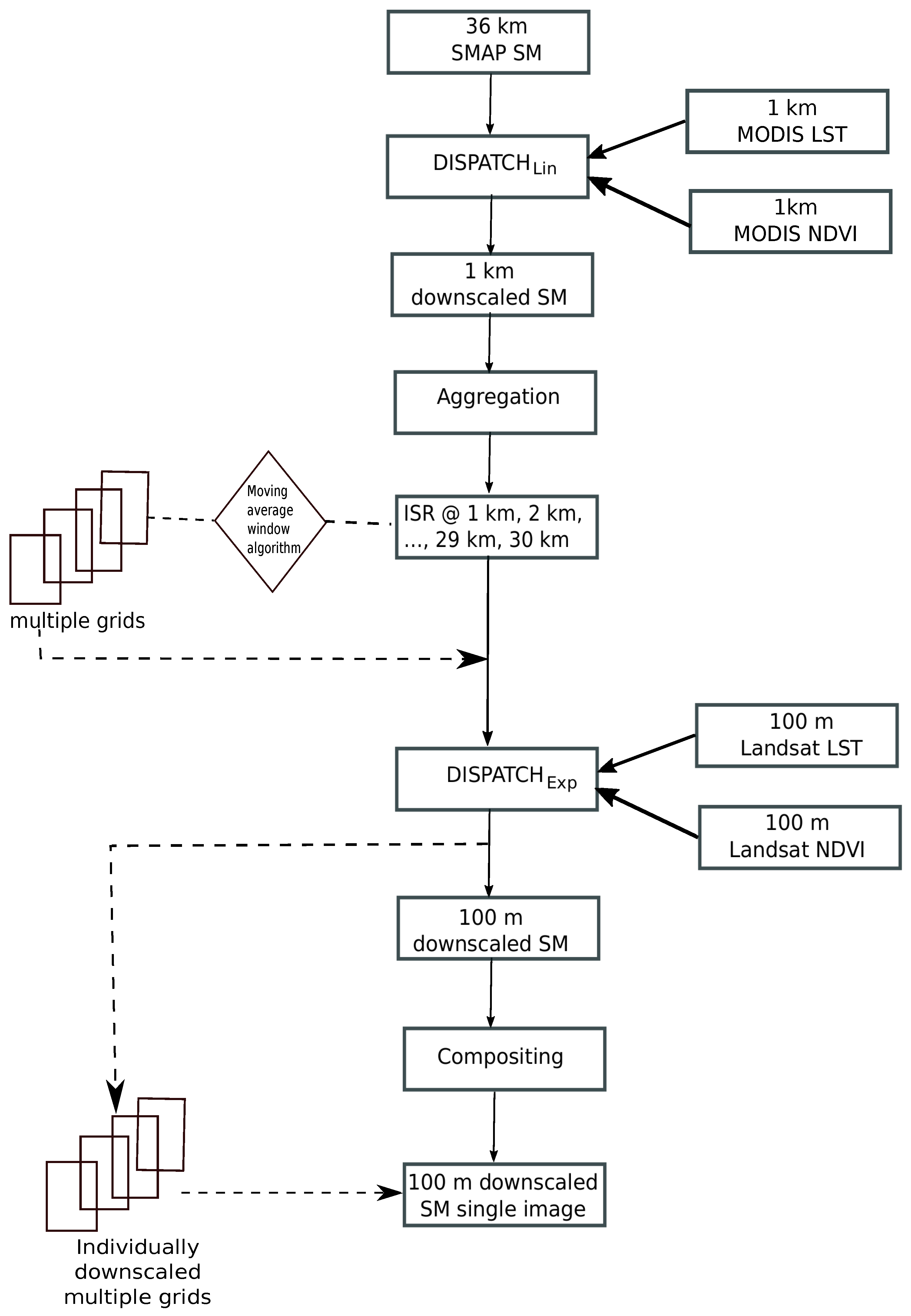
2.5. Sequential Downscaling

Figure 3 presents a flow chart of the sequential disaggregation in 3 successive steps. SMAP SM is first disaggregated from 36 km to 1 km resolution using MODIS data and DISPATCH L i n algorithm. Then the 1 km resolution SM is aggregated at ISR. Next, the ISR SM is further disaggregated at 100 m resolution using Landsat data and DISPATCH E x p algorithm.
The reason for the selection of a range of ISRs is associated with the contextual nature of DISPATCH, which makes the determination of temperature endmembers i.e., T s , d r y and T s , w e t , and hence the 100 m resolution Landsat-derived SEE, dependent on the spatial extent [59]. In particular, the larger the spatial extent, the more heterogeneous the surface becomes. Therefore, the accuracy in temperature endmembers should increase with the spatial extent, as long as the meteorological forcing data remain relatively uniform (underlying assumption of the contextual analysis). Therefore, an optimal ISR in terms of SM accuracy at the 100 m resolution appears to be a compromise between (i) the accuracy in temperature endmembers and (ii) the gap between LR and HR. One major objective of this paper is to check the sensitivity of the sequential approach to ISR and to propose an optimal ISR for routine application.
Figure 4 plots the LST- f v feature space obtained for 100 m resolution Landsat data collected on DOY 38 and for 4 distinct spatial extents within the study area: 1 km, 3 km, 10 km, and 30 km. It can be seen that the range of LST and f v values increases with the spatial extent over which the temperature endmembers are estimated. The mean LST is also larger for the smaller ISR values; which may induce bias in the disaggregation. If we consider that the temperature endmembers retrieved from the 10 km pixel resemble the real dry and wet soil temperatures, then more uncertainty can be seen while decreasing the spatial extent. An inaccurate representation of the wet/dry and bare/vegetated soil conditions within the spatial extent (ISR pixel) will directly affect the calculation of temperature endmembers and hence the thermal-derived SEE, and finally downscaling. Conversely, when extending (too much) the spatial extent, the spatial variability of air temperature (and wind speed notably) may reach a critical level that invalidates the contextual approach’s assumption regarding the uniformity of meteorological forcing. In this respect, the LST- f v feature space plotted in Figure 4 for a spatial extent of 30 km indicates that two trapezoidal shapes appear separately, which may be a signature of sub-areas having different meteorological forcing. Both constraints (heterogeneity of surface conditions and homogeneity of meteorological conditions) actually represent an important rationale for implementing a sequential method with an ISR between the 1 km and SMAP resolution.
Once the spatial extent of the LST- f v feature space and the algorithm for estimating temperature endmembers have been defined, one can check the linearity or non-linearity of the SEE(SM) model and its consistency with the SEE(LST) model. Figure 5 plots Landsat-derived SEE as a function of in-situ SM for DOY 14. The predictions of the SEE(SM) model of Equation (7) is also plotted, with S M p estimated by setting in Equation (8) LR SM and LR SEE to the mean in situ SM and the mean Landsat-derived SEE, respectively. The correlation coefficient and slope between SEE(SM) and SEE(LST) estimates are 0.87 and 0.41 for DISPATCH E x p algorithm. For comparison purposes, Figure 5 also plots SEE(SM) and SEE(LST) predictions for the DISPATCH L i n algorithm. The correlation coefficient and slope between both models are 0.87 and 0.17 respectively. Even though the correlation coefficient shows similar values for both DISPATCH L i n and DISPATCH E x p , the slope is significantly lower than that for DISPATCH E x p . Those results are fully consistent with our approach to make the SEE(SM) non-linear (using the exponential form of [57]) and to improve the temperature endmembers algorithm [56] of the SEE(LST) model within the new DISPATCH E x p downscaling algorithm.

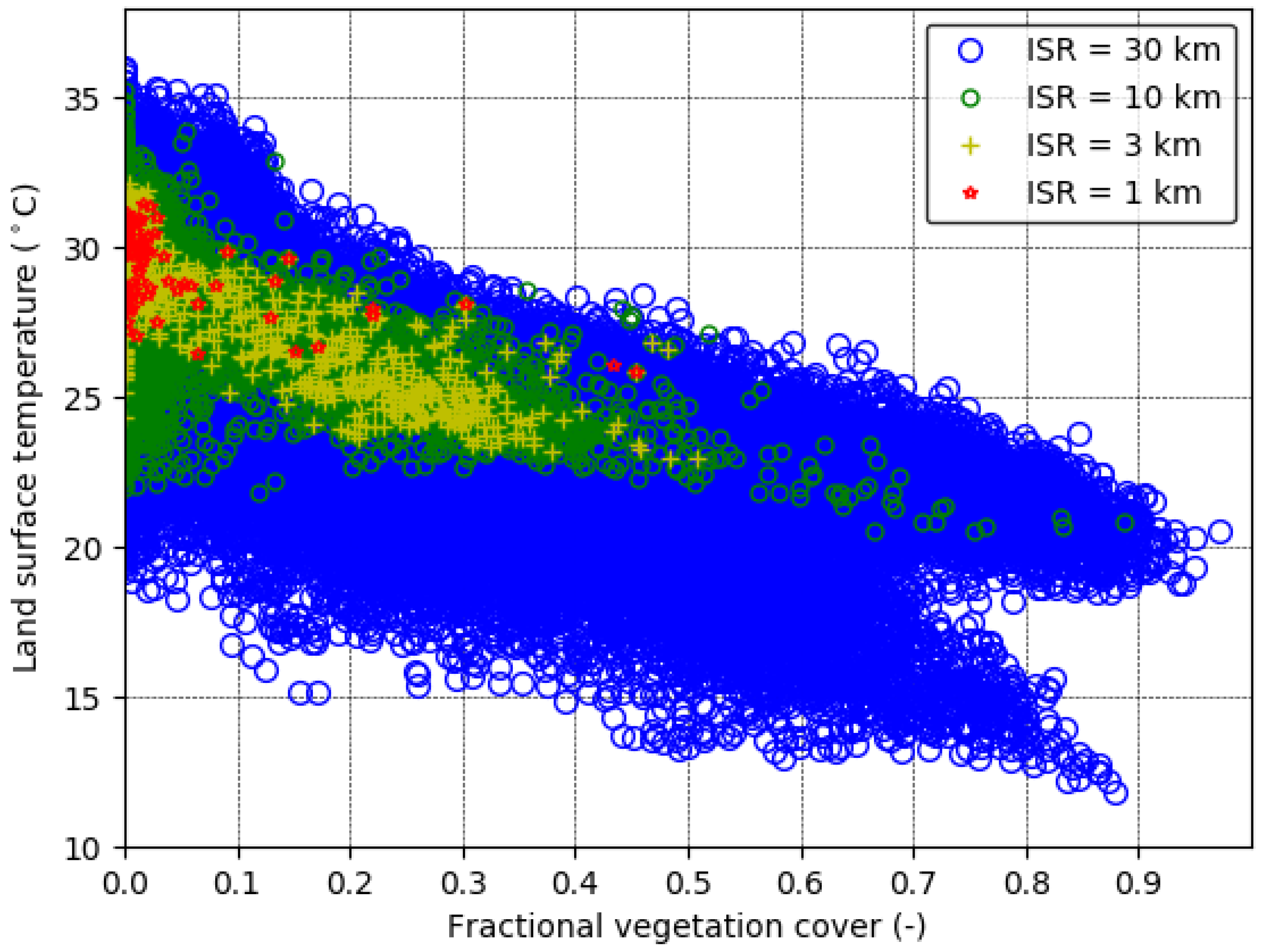
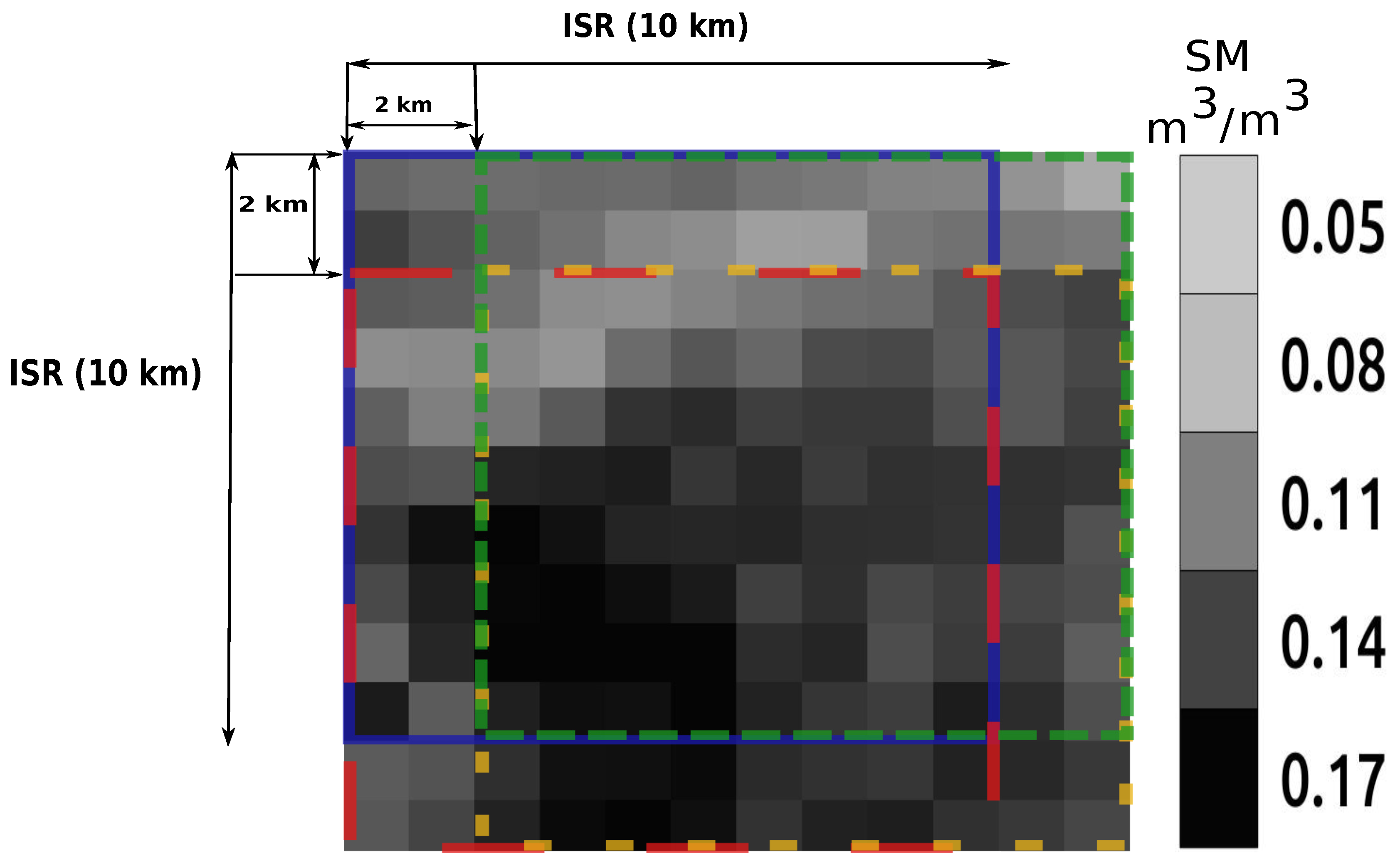
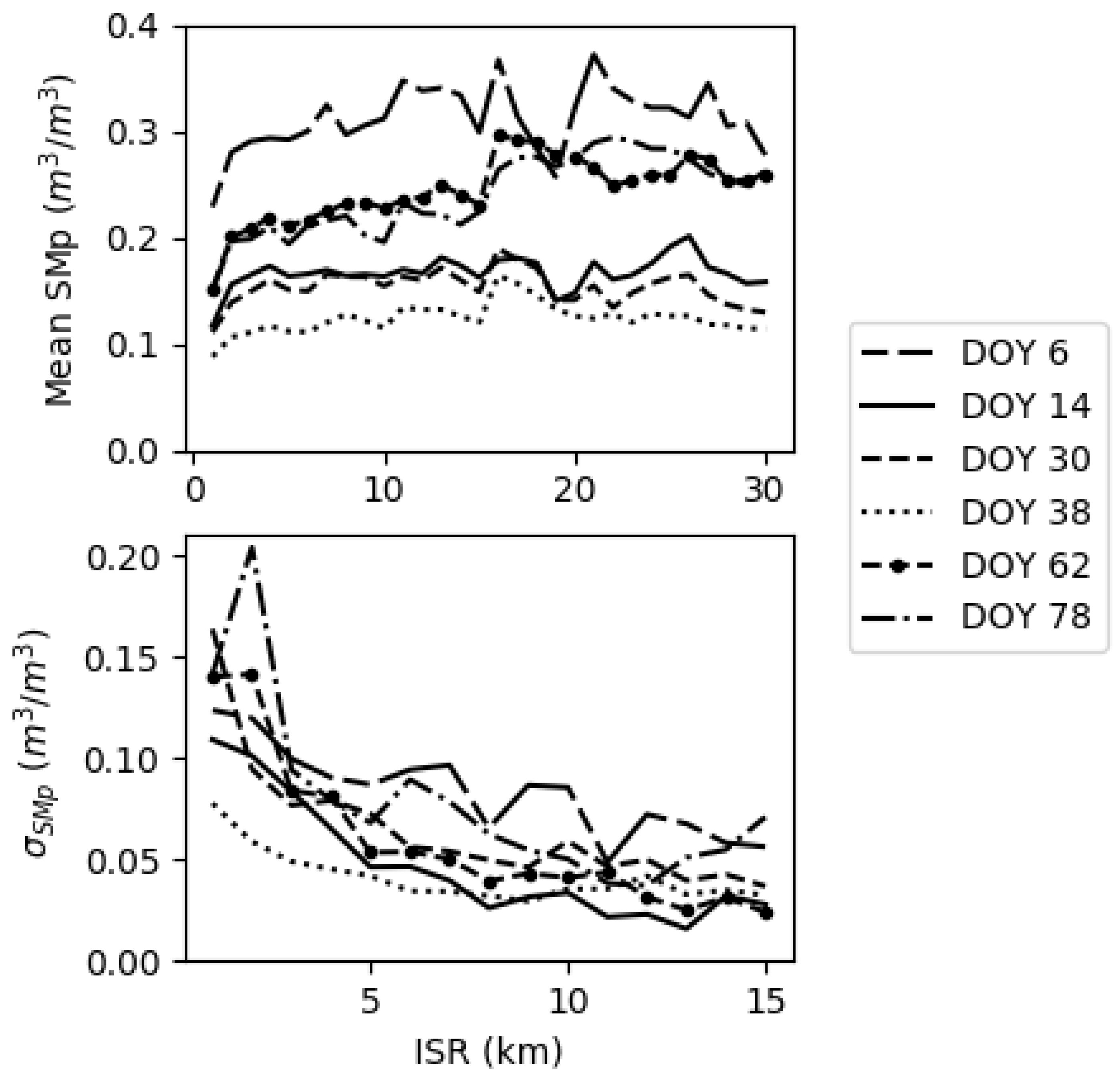
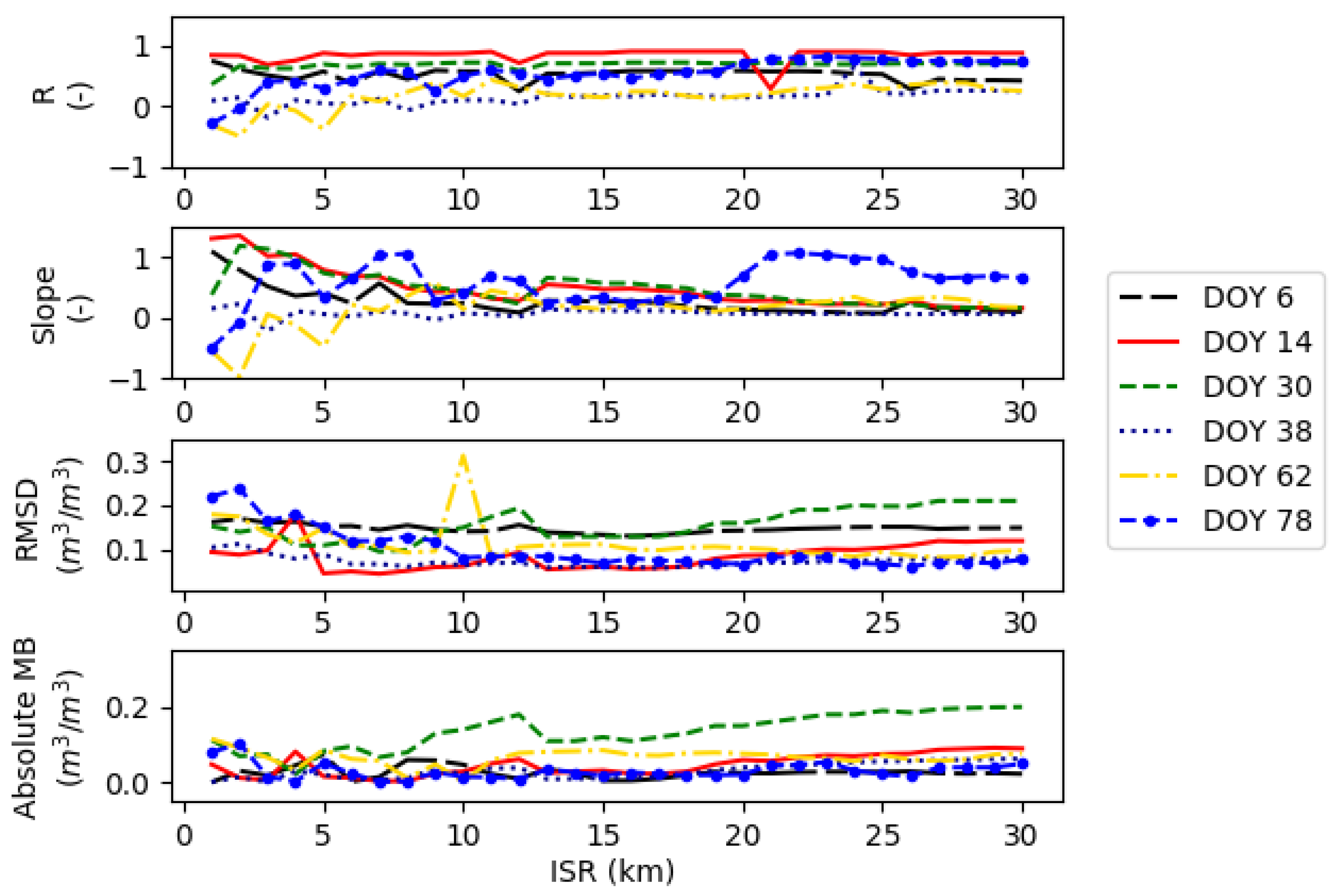
2.6. Inclusion of Multiple ISR Grids

The use of multiple LR grids as input to disaggregation approaches has been proposed in Hoehn et al. [60] and Merlin et al. [26]. Hoehn et al. [60] compared downscaling results obtained from single coarse resolution grid (using fixed window) and using multiple overlapping coarse resolution grids (by shifting windows). Shifting windows using multiple grids showed better performance as compared to the fixed window case with respect to error and smoothness.
In this paper, we propose to define multiple ISR grids as an input to DISPATCH E x p as in Merlin et al. [26] and Hoehn et al. [60]. However, one difference herein is that the multiple ISR grids are built from actual observations at the (higher) 1 km resolution and consequently, they are derived neither from the LR overlapped observations [26], nor from the oversampling of LR (SMAP) observations [60].
Figure 6 gives an illustration of the moving average window algorithm, over the 1 km resolution grid of the DISPATCH L i n output data. The algorithm successively shifts an ISR grid in both directions (east-west and north-south) of a predefined constant distance. In the diagram of Figure 6, ISR is set to 10 km and the distance separating the so generated ISR grids is set to 2 km. Once the multiple grids have been generated, they are independently used as input to DISPATCH E x p . As a first step, multiple ISR SM grids are thus overlapped with 100 m resolution Landsat data and disaggregated separately to get multiple 100 m resolution disaggregated SM images. As a second step, the separate 100 m resolution downscaled SM images are composited (simple average) to produce a single 100 m resolution SM disaggregated image.

3. Results

This section analyzes the potential of the sequential downscaling approach by investigating (1) the method calibration (2) the method accuracy for a range of ISR values using the single grid algorithm, and (3) the usefulness of the multiple grid (compared to the single grid) algorithm.

3.1. Calibration

The calibration of S M p parameter in Equation (8) is undertaken using the DISPATCH L i n data sets derived from SMAP, on each date when Landsat data are available. Figure 7 plots S M p as a function of ISR for each Landsat overpass date. The mean and standard deviation of retrieved S M p are computed within the 30 km by 30 km study domain. It can be seen that for all dates, the retrieved S M p behaves quite similarly with respect to ISR. It sharply increases for an ISR increasing from 1 km to 3–4 km and then keeps a relatively stable value for ISR values ranging between 3–4 km and 30 km. Note that significant fluctuations of S M p are observed for ISR values larger than 15 km, due to the bounded extent of the study area i.e., the mean S M p is computed using a single retrieved value. However, the S M p value after convergence is not fully consistent for different dates. In fact, the estimation of S M p in Equation (8) mainly depends on LR SM and SEE data, so that any error in SMAP SM and Landsat-derived SEE estimates leads to temporal variabilities in retrieved S M p .
The standard deviation of the retrieved S M p values within the 30 km by 30 km area is also plotted as a function of ISR ranging from 1 km to 30 km. It can be seen that the spatial variability in retrieved S M p significantly decreases in the higher ISR range to reach a minimum for ISR values larger than 10 km. Note that the standard deviation becomes zero for ISR equal or larger than 15 km (not shown in the graph) because in such cases, a single ISR pixel is obtained within the whole extent of the (30 km wide) study area. Figure 8 presents the images of S M p retrieved for ISR equal to 1 km, 3 km, 10 km, and 30 km. The spatial variability of S M p strongly increases when ISR decreases and tends to 1 km and the average of 1 km resolution S M p is significantly different from the S M p retrieved over 10 km ISR pixels. Such behavior is explained by the non-linear impact of LR SEE on S M p (see Equation (8), and by the non-representativeness of temperature endmembers for ISR lower than 5 km.
From the results presented in Figure 7 and Figure 8, it can be concluded that (1) the retrieved S M p is spatially and temporally representative for ISR equal to or larger than 10 km, and (2) significant spatial/temporal variabilities of S M p (associated with uncertainties in temperature endmembers) and non linear effects (associated with the non linear SEE(SM) relationship) are obtained for ISR lower than 5 km.

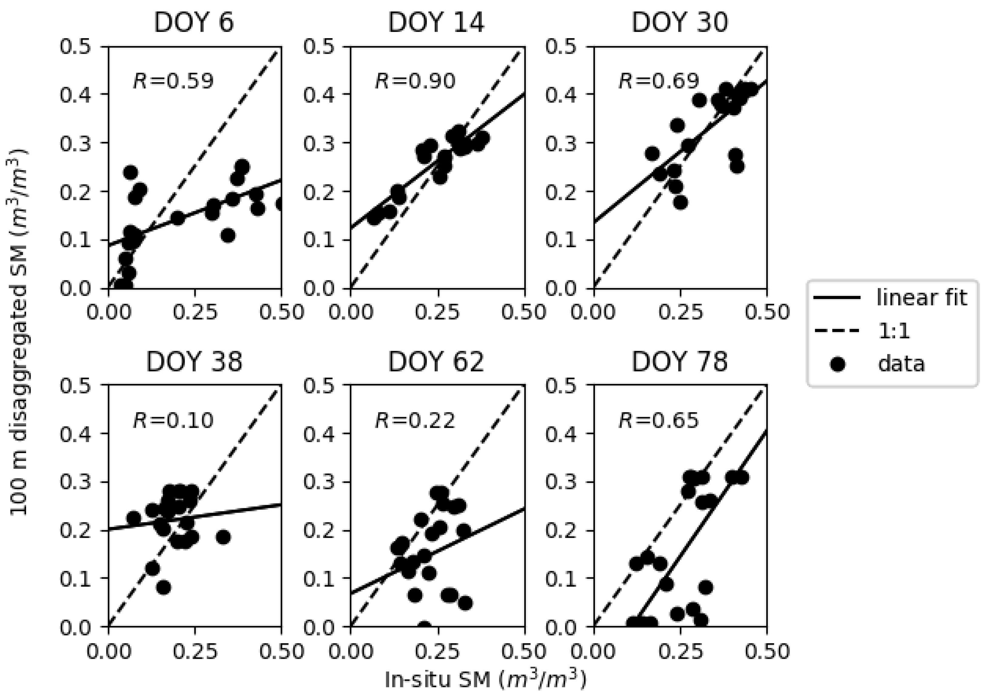
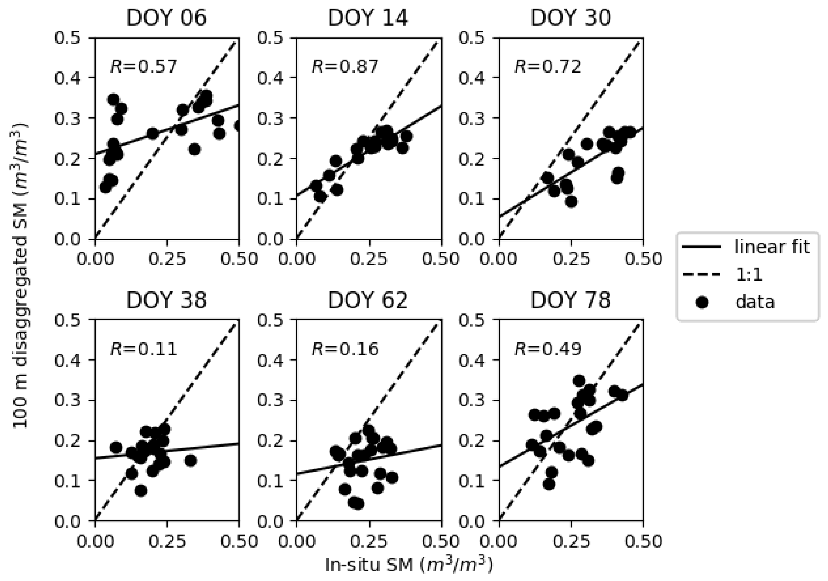
3.2. Evaluation of 100 m Disaggregated SM

The S M p retrieved from Equation (8) is first used to calculate the derivative from the average of Equations (9) and (10). A range of different ISR values is then chosen to evaluate the sensitivity of 100 m resolution disaggregated SM to ISR. To do so, the 1 km resolution disaggregated SM (the output of DISPATCH L i n ) is aggregated to 1, 2, 3, ……, and 30 km and in each case, the aggregated ISR SM together with its associated spatial extent is used as an input to DISPATCH E x p . Such a sensitivity analysis is undertaken for each SMAP overpass date, separately.
The statistical comparison in terms of correlation coefficient (R), slope of the linear regression (slope), root mean square deviation (RMSD) and absolute mean bias (MB) between DISPATCH E x p disaggregated SM and in-situ SM is illustrated in Figure 9 for ISR ranging from 1 to 30 km for each sampling date. The temporal variability (standard deviation) of R and of the slope of the linear regression is relatively large in the lower range of ISR values. The slope gets even negative values for ISR lower than 5 km on several dates, while the slope is always positive for ISR larger than 10 km. This result is consistent with the stability of S M p retrievals observed previously for ISR larger than 5 km.
When considering the full ISR range (1–30 km), and despite the date-to-date variability, a slight general increase of R is obtained in the 1–10 km range, whereas it keeps an approximately constant value for larger ISRs. Regarding the slope of the linear regression, an opposite finding is obtained. For ISR values larger than 5 km, the slope keeps decreasing with a value at ISR = 30 km mostly very close to zero. Note that the sudden increase of the slope for ISR = 20 km on DOY 78 is due to the fact that statistical results are obtained from a single (unrepresentative) ISR pixel that fits into the 30 km by 30 km study area. The decrease of the slope is attributed to the gap between the LR and the HR, which increases with ISR. In fact, the disaggregation efficiency (as defined in [61]) is expected to decrease with the LR to HR ratio, due to the decrease of the spatial variability represented at HR by the LR observation. The slope of the linear regression was actually found to be a good indicator of the disaggregation efficiency [61], consistent with the results presented in Figure 9. A second important impact of ISR is the increase of the absolute MB between the 100 m resolution disaggregated and in situ SM, especially in the 10–30 km range. The worsening of downscaling performances (in terms of the slope of the linear regression and MB) in the 10–30 km range is due to the linear approximation of the downscaling relationship (Equation (3). An optimal ISR is thus found at around 10 km. Optimal results in terms of RMSD between 100 m resolution and in-situ SM is actually obtained for ISR close to 10 km. Therefore, ISR set to 10 km throughout the rest of the paper.
For illustration purposes, Figure 10 represents the sequential downscaling of SM from SMAP data collected on DOY 38: the disaggregation of SMAP SM to 1 km resolution, the aggregation of the 1 km resolution disaggregated SM to ISR (10 km), and the disaggregation of ISR SM to 100 m resolution. It is reminded that the extra aggregation step is undertaken (i) to increase the representativeness/accuracy of the temperature endmembers extrapolated from the LST- f v feature space, (ii) to increase the stability of the disaggregation calibration (via the S M p retrieval) and (iii) to reduce random uncertainties in the ISR SM used as input to DISPATCH E x p .
As a first evaluation of the disaggregation at 100 m resolution independently from the uncertainty in SMAP data, DISPATCH E x p is run for all sampling dates (DOY 6, 14, 30, 38, 62 and 78) by setting the ISR observation to a fraction of the mean (daily areal average of) in-situ SM. By considering that the average of all in-situ SM measurements is representative of the SM over the irrigated area and that the SM over dry land is about 0, a rough estimate of the LR SM is derived as half the mean in situ measurements (the fraction of dry land in the 10 km ISR pixel covering the experimental fields is about 50%). Figure 11 plots the 100 m resolution disaggregated SM versus in situ measurements. Statistical results in terms of R, slope of the linear regression, absolute MB and RMSD are reported in Table 1 for synthetic LR. R is in the range 0.6–0.9 for four dates (DOY 6, 14, 30 and 78), while it is in the range 0.1–0.2 on two dates (DOY 38 and 62). In terms of correlation, better results are obtained on the sampling dates with a larger spatial variability in SM measurements, and reciprocally, poorer results are obtained when SM is relatively uniform at the sub-pixel scale. In terms of bias, however, relatively low absolute MB (lower than 0.03 m 3 /m 3 ) is obtained except for DOY 6, 62 and 78 with an absolute MB of 0.07, 0.08 and 0.11 m 3 /m 3 , respectively. The reason is that the mean in situ measurements (weighted by the fraction of irrigated land) may not be fully representative of the real SM at the ISR (10 km) scale, as irrigation is not applied uniformly within the irrigated perimeter. Nevertheless, the application of DISPATCH E x p to synthetic LR (ISR) SM data allows for assessing the performance of the downscaling methodology independently of SMAP data and DISPATCH L i n algorithm. We conclude that DISPATCH E x p is relatively efficient when the sub-pixel variability is larger than 0.06 m 3 /m 3 .
Next, DISPATCH E x p is tested using SMAP data (ISR is still set to 10 km in the sequential downscaling). Figure 12 represents the comparison between DISPATCH E x p and in situ SM and Table 1 for SMAP single grid reports the associated statistical results. It can be seen that results are not significantly degraded in terms of R compared to the case when using synthetic LR observation as input to DISPATCH E x p (see Table 1). In fact, the sub-pixel variability of SM is represented by the Landsat-derived SEE in both real and synthetic cases, which explains similar R results. However, the DISPATCH L i n data derived from SMAP data may involve LR differences in terms of MB and RSMD at 100 m resolution.

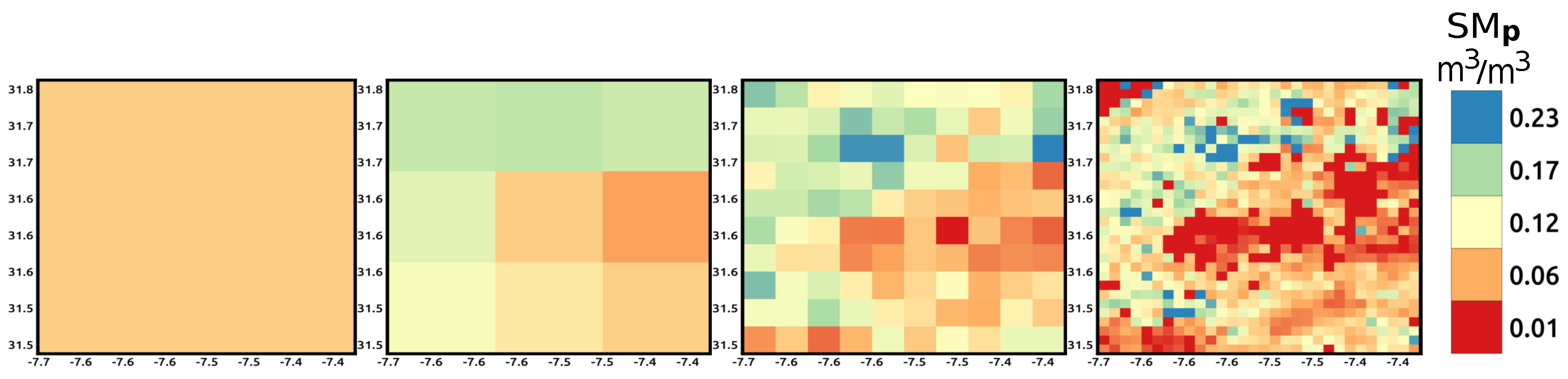
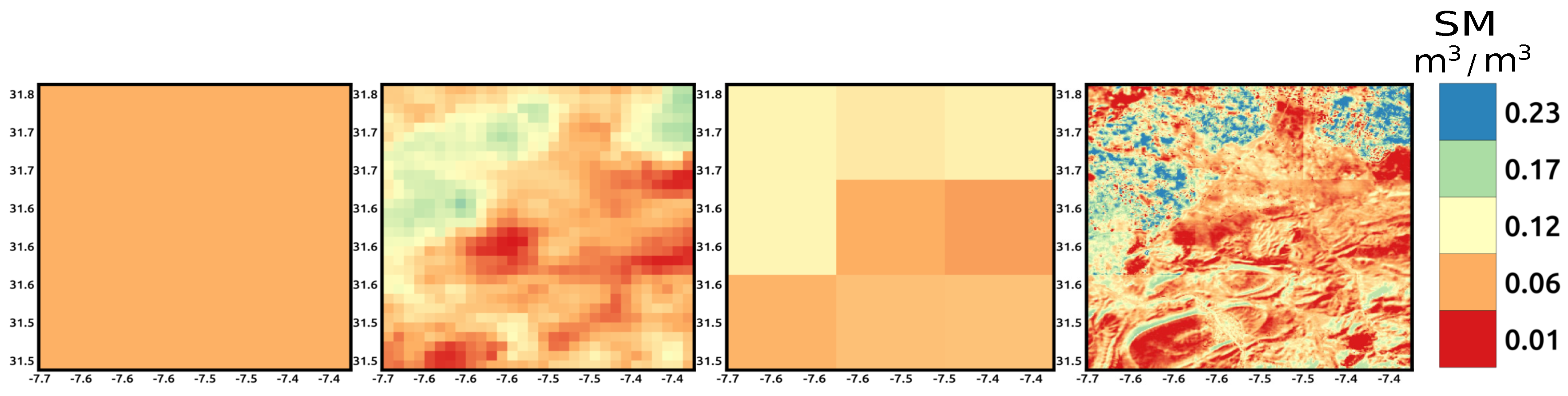
3.3. Reducing Boxy Artifact

As demonstrated and discussed above, setting an ISR between the SMAP and Landsat resolutions has many advantages in terms of accuracy and robustness of DISPATCH E x p . However, one drawback with an ISR equal to 10 km, is that the ISR grid may be still apparent in the 100 m resolution disaggregated image. Such effects are called boxy artifacts [62]. To reduce these boxy artifacts and to potentially increase the accuracy in 100 m disaggregated SM, a Monte-Carlo sampling method is proposed as an extra step in the pre and post-processing of input/output data of DISPATCH E x p .
The preprocessing steps include: (i) selecting 10 km resolution SM pixels such that an equal number of HR (Landsat) pixels falls within each ISR pixel (ii) shifting the 10 km ISR pixels with a distance of 2 km in east-west and north-south directions, so as to generate a set of 25 ISR SM images, (iii) overlapping each image with HR Landsat optical/thermal data, and (iv) disaggregating individually each ISR image to 100 m resolution. Therefore, a set of 25 possible disaggregated 100 m SM images is obtained. The post-processing step consists in combining the 25 disaggregated SM images. The simple averaging is used to produce a single 100 m disaggregated image.
The multiple-grid procedure illustrated in Figure 6 is applied over our 30 km by 30 km study area for SMAP data and for each date separately. Figure 13 presents the 100 m resolution SM disaggregated images by applying the single grid and multiple grid algorithms for each date separately. It can be seen on DOY 6, 38 and 78 that the boxy artifacts at 10 km resolution present on the image obtained using the single grid algorithm have completely disappeared in the multiple grids application. Note that the boxy artifacts are not visible for the other dates due to strips (data gaps) present in the Landsat 7 images. The moving window algorithm also smoothens the disaggregated image at the image borders. Especially, the errors that generally occur at the corners of the image due to sudden changes in temperature endmembers and coarse scale SM are reduced. The composited image is of better quality by reducing the random errors associated with the uncertainty in LR observations and the disaggregation methodology (involving non-linear relationships between SEE and SM), which make the disaggregated image more realistic than using the single grid algorithm.
Table 2 reports the standard deviation of 100 m resolution disaggregated SM within each image for the single and multiple grid algorithms, separately. The standard deviation is systematically lower when applying multiple grids for all the dates. It means that the multiple grid application significantly reduces the variabilities attributed to random uncertainties in DISPATCH E x p input data. A quantitative comparison between 100 m disaggregated SM and in situ measurements is also proposed in Table 1 for SMAP multiple grid. By comparing the statistical results from the single grid and multiple grid (Table 1) algorithm, it can be seen that both the R and slope of the linear regression between 100 m resolution disaggregated and in situ SM are generally increased by applying multiple grids. Therefore, the proposed moving window method not only provides continuous SM images but also increases the efficiency of the disaggregation approach at 100 m resolution.

4. Discussion

High spatial resolution soil moisture data are fundamental for hydro-agricultural purposes as well as for other kind of applications. The DISPATCH method sequentially applied to SMAP data at 1 km resolution (using MODIS) and at 100 m resolution (using Landsat) has potential for providing such data. However, the performance of the approach may depend on the surface and atmospheric conditions. In addition, the temporal resolution of 100 m resolution DISPATCH data is currently limited by (i) the repeat cycle (16 days) of Landsat and (ii) the cloud free conditions required to use optical/thermal data. This section thus discusses the applicability and expected performance of DISPATCH in a context wider than our semi-arid irrigated study area.
The disaggregation of coarse scale soil moisture data is still a relatively recent research avenue [24], and consequently, few studies have compared the performance of existing methods. Sabaghy et al. [23] undertook the first comprehensive and systematic comparison study of several radar-based and optical/thermal-based SM downscaling methods. The SM downscaled from SMOS and SMAP data were evaluated against in situ as well as airborne SM estimates using the AACES data set in Southeastern Australia. DISPATCH was among the most efficient downscaling methods, especially when evaluating the spatial representation at 1 km resolution. The results presented in this paper are consistent with Sabaghy et al. [23] and previous validation exercises of DISPATCH. However, several intrinsic limitations common to optical/thermal-based downscaling approaches needs to be acknowledged, while several weaknesses specific to DISPATCH could be addressed in the future.
In this study, the mean RMSD (about 0.10 m 3 /m 3 ) between disaggregated SMAP and in situ SM is relatively large and need to be interpreted in terms of bias and precision and to be compared with the spatio-temporal variability of SM existing within the study area. First, the mean RMSD is mostly explained by daily biases (mean bias of about 0.08 m 3 /m 3 ) while the slope of the linear regression between disaggregated and in-situ SM is systematically and significantly positive. Second, the spatial variability of SM at 100 m resolution is extreme over the irrigated area with surface conditions ranging from bone dry to soil fully saturated. Over the sampled area, the minimum and maximum measured SM value was 0.03 to 0.45 m 3 /m 3 , respectively. In such highly heterogeneous areas, relatively large errors in SM estimates are thus expected. It is however reminded that the disaggregation error should be smaller than the actual SM variability, as an indicator of the relevance of such disaggregated SM data [63].
It is reminded that the DISPATCH methodology relies on the relationship between moisture and the LST. LST is in fact a signature of the surface energy balance, which is highly linked to the evaporation flux and the associated soil water availability. NDVI data are used in DISPATCH to partition the LST into its soil and vegetation components, given that the soil temperature is more directly linked to the top SM while the vegetation temperature is related to the deeper root zone SM [26]. Therefore, the application of the DISPATCH method over irrigated regions is fully relevant. In our study area, flood irrigation consists in applying about 60 mm in several (typically 4) hours so as to flood the entire field. However, the irrigation water rapidly infiltrates into the soil so that there is little chance that the Landsat satellite actually “sees” any inundated field (although it may potentially happen), all the more as the typical frequency of flood irrigations is one every 3 weeks. The flood irrigation technique is still widely applied in Morocco and in many developing countries where traditional practices persist. Note that the application of DISPATCH over drip irrigated crops would require thermal data with a high repeat cycle, consistent with the irrigation frequency for the drop-by-drop technique.
One major limitation of DISPATCH is the availability of optical/thermal data. DISPATCH has been tested mostly under arid or semi-arid regions where the cloud cover is rather small. In particular, the cloud cover of the Haouz plain is about 40% from January to May while its overall yearly percentage is 30% [64]. The 100 m resolution downscaled SM time series is thus expected to be much less dense over other regions having a larger cloud cover. In addition, as DISPATCH relies on the LST-moisture relationship, the performance of downscaling depends on the atmospheric evaporative demand. Therefore, testing its applicability to different climatic conditions will be needed in the future, notably by identifying moisture-limited and energy-limited regions.
Other limitations specific to DISPATCH includes the non-linear behavior of the SEE(SM) relationship and the so-called “boxiness” within the downscaled image. From Figure 11 and Figure 12, relationships between disaggregated and in-situ SM appear to be non-linear on several dates (DOY 6 notably). This is explained by (i) the non-linear behavior of SEE for a range of SM values and (ii) the linear approximation of DISPATCH around the LR SM (Equation (3). It seems that using a non-linear SEE(SM) model in Equation (3) is not sufficient to represent the nonlinear SEE(SM) relationship when the SM variability is extreme. Future studies will address this issue by, for instance, correcting the SEE(SM) relationship when the sub-pixel SM variability is larger than a given threshold. Regarding the “boxiness” within the image, it is a relatively small effect compared to the spatial variability of SM represented by the DISPATCH method. Quantitatively, the RMSD between the SM produced from single grid and multiple grid applications is 0.019 m 3 /m 3 , while the standard deviation of disaggregated SM within the study area is 0.089 and 0.075 m 3 /m 3 for the single and multiple grid case, respectively. In fact, as shown in Figure 13 the single grid application (without removing the boxiness within the image) already provides 100 m resolution SM images with borders between ISR pixels very consistent from one ISR pixel to another adjacent ISR pixel. Therefore, the stepwise method proposed in this paper does transfer in a satisfying manner the SM information from the 36 km SMAP resolution to the targeted 100 m resolution.

5. Conclusions

A stepwise disaggregation approach of SMAP SM is developed at 100 m resolution using the DISPATCH methodology and Landsat data. SMAP SM is first disaggregated from 36 km to 1 km resolution using MODIS data and DISPATCH L i n algorithm. Then the 1 km resolution SM is aggregated as ISR. Next, the ISR SM is further disaggregated at 100 m resolution using Landsat data and DISPATCH E x p algorithm. In order to take into account the increase of resolution, the new DISPATCH E x p algorithm brings several innovations compared to the DISPATCH version currently implemented at CATDS (DISPATCH L i n ) in two aspects: (i) the SEE is a non-linear function of SM, and (ii) the SEE(LST) model is improved by better constraining the determination of temperature endmembers. The approach is evaluated using in situ measurements collected on the dates with concurrent SMAP, MODIS, and Landsat overpasses.
ISR is varied between 1 km and 30 km with a 1 km step, and sensitivity of the calibration parameter (SMp) of DISPATCHExp to ISR is analyzed. The retrieved S M p is spatially and temporally representative for ISR equal or larger than 10 km, while significant spatial variabilities of S M p (associated with uncertainties in temperature endmembers) and non-linear effects (associated with the non-linear SEE(SM) relationship) are obtained for ISR lower than 5 km. Optimal results in terms of RMSD between 100 m resolution and in situ SM are obtained for ISR close to 10 km. Therefore, the two-step disaggregation is more efficient than the direct disaggregation from SMAP to 100 m resolution. This is due to the trade-off existing between the performance (increasing with the ISR and its sub-pixel variability) of the contextual-based DISPATCH method and the statistical match (decreasing with ISR) between ISR remotely sensed and field-scale SM estimates. The correlation coefficient between 100 m resolution disaggregated and in situ SM ranges between 0.5–0.9 for four out of the six sampling dates. Better results are obtained on the sampling dates with a larger spatial variability in SM measurements, and reciprocally, poorer results are obtained when SM is relatively uniform at the sub-pixel scale.
Finally, a new method is proposed to reduce boxy artifacts at 10 km resolution in 100 m resolution disaggregated SM images. The multiple grid application perfectly smoothens the composited 100 m resolution disaggregated SM image and, in addition, quantitatively improves the efficiency of the downscaling approach by increasing the correlation coefficient and slope of the linear regression between 100 m resolution disaggregated and in situ SM.
The DISPATCH-based sequential disaggregation scheme has the advantage of being independent on ground-based measurements, as all input parameters (i.e., temperature endmembers and S M p ) are calibrated using remote sensing data. However, the unavailability of optical/thermal (MODIS/Landsat) data in cloudy conditions is still a severe limitation for operational applications. One key avenue for producing SM data sets at high spatial-temporal resolution could be the synergy with radar-based approaches [18,24]. Recently, Amazirh et al. [49] calibrated the main parameters of a radar-based SM retrieval method using a thermal-derived SM proxy. In the same vein, the 100 m resolution DISPATCH E x p SM data sets obtained from SMAP data on MODIS/Landsat clear sky days could represent a cornerstone in the construction of synergies between passive/active microwave and optical/thermal data.

Author Contributions

Conceptualization, N.O. and O.M.; methodology, N.O. and O.M.; validation N.O. and O.M.; supervision O.M.; investigation, N.O.; data curation, N.O., L.O.-G., B.A.H. and A.A.; writing—original draft preperation, N.O., O.M.; writing—review and editing, N.O., O.M., B.M., C.S., A.A.B., M.J.E. and S.E.-R.

Funding

This study was supported by the European Commission Horizon 2020 Programme for Research and Innovation (H2020) in the context of the Marie Sklodowska-Curie Research and Innovation Staff Exchange (RISE) action (REC project, grant agreement no: 645642 followed by ACCWA project, grant agreement no.: 823965).

Acknowledgments

We would like to thank the National Aeronautics and Space Administration (NASA) for freely providing the data. We would also like to thank the reviewers for their valuable comments.

Conflicts of Interest

The authors declare no conflict of interest.

References

  1. Bisquert, M.; Sánchez, J.; López-Urrea, R.; Caselles, V. Estimating high resolution evapotranspiration from disaggregated thermal images. Remote Sens. Environ. 2016, 187, 423–433. [Google Scholar] [CrossRef]
  2. Maurer, E.P.; Wood, A.; Adam, J.; Lettenmaier, D.P.; Nijssen, B. A long-term hydrologically based dataset of land surface fluxes and states for the conterminous United States. J. Clim. 2002, 15, 3237–3251. [Google Scholar] [CrossRef]
  3. Koster, R.D.; Dirmeyer, P.A.; Guo, Z.; Bonan, G.; Chan, E.; Cox, P.; Gordon, C.; Kanae, S.; Kowalczyk, E.; Lawrence, D.; et al. Regions of strong coupling between soil moisture and precipitation. Science 2004, 305, 1138–1140. [Google Scholar] [CrossRef] [PubMed]
  4. Wang, K.; Dickinson, R.E. A review of global terrestrial evapotranspiration: Observation, modeling, climatology, and climatic variability. Rev. Geophys. 2012, 50. [Google Scholar] [CrossRef]
  5. Entekhabi, D.; Njoku, E.G.; O’Neill, P.E.; Kellogg, K.H.; Crow, W.T.; Edelstein, W.N.; Entin, J.K.; Goodman, S.D.; Jackson, T.J.; Johnson, J.; et al. The soil moisture active passive (SMAP) mission. Proc. IEEE 2010, 98, 704–716. [Google Scholar] [CrossRef]
  6. Kerr, Y.H.; Waldteufel, P.; Wigneron, J.P.; Delwart, S.; Cabot, F.; Boutin, J.; Escorihuela, M.J.; Font, J.; Reul, N.; Gruhier, C.; et al. The SMOS mission: New tool for monitoring key elements ofthe global water cycle. Proc. IEEE 2010, 98, 666–687. [Google Scholar] [CrossRef]
  7. Wagner, W. Operational Readiness of Microwave Remote Sensing of Soil Moisture: An Update. In Proceedings of the EGU General Assembly 2010, Vienna, Austria, 2–7 May 2010; Volume 12, p. 2636. [Google Scholar]
  8. Kerr, Y.H.; Waldteufel, P.; Wigneron, J.P.; Martinuzzi, J.; Font, J.; Berger, M. Soil moisture retrieval from space: The Soil Moisture and Ocean Salinity (SMOS) mission. IEEE Trans. Geosci. Remote Sens. 2001, 39, 1729–1735. [Google Scholar] [CrossRef]
  9. Schmugge, T. Applications of passive microwave observations of surface soil moisture. J. Hydrol. 1998, 212, 188–197. [Google Scholar] [CrossRef]
  10. Schmugge, T.; Jackson, T. Mapping surface soil moisture with microwave radiometers. Meteorol. Atmos. Phys. 1994, 54, 213–223. [Google Scholar] [CrossRef]
  11. Bindlish, R.; Crow, W.T.; Jackson, T.J. Role of passive microwave remote sensing in improving flood forecasts. IEEE Geosci. Remote Sens. Lett. 2009, 6, 112–116. [Google Scholar] [CrossRef]
  12. Kerr, Y.H.; Waldteufel, P.; Richaume, P.; Wigneron, J.P.; Ferrazzoli, P.; Mahmoodi, A.; Al Bitar, A.; Cabot, F.; Gruhier, C.; Juglea, S.E.; et al. The SMOS soil moisture retrieval algorithm. IEEE Trans. Geosci. Remote Sens. 2012, 50, 1384–1403. [Google Scholar] [CrossRef]
  13. Malbéteau, Y.; Merlin, O.; Molero, B.; Rüdiger, C.; Bacon, S. DisPATCh as a tool to evaluate coarse-scale remotely sensed soil moisture using localized in situ measurements: Application to SMOS and AMSR-E data in Southeastern Australia. Int. J. Appl. Earth Obs. Geoinf. 2016, 45, 221–234. [Google Scholar] [CrossRef]
  14. Walker, J.P.; Houser, P.R. Requirements of a global near-surface soil moisture satellite mission: Accuracy, repeat time, and spatial resolution. Adv. Water Resour. 2004, 27, 785–801. [Google Scholar] [CrossRef]
  15. Hawley, M.E.; Jackson, T.J.; McCuen, R.H. Surface soil moisture variation on small agricultural watersheds. J. Hydrol. 1983, 62, 179–200. [Google Scholar] [CrossRef]
  16. Fang, B.; Lakshmi, V.; Bindlish, R.; Jackson, T.J. Downscaling of SMAP soil moisture using land surface temperature and vegetation data. Vadose Zone J. 2018, 17, 1. [Google Scholar] [CrossRef]
  17. Chen, N.; He, Y.; Zhang, X. NIR-Red Spectra-Based Disaggregation of SMAP Soil Moisture to 250 m Resolution Based on OzNet in Southeastern Australia. Remote Sens. 2017, 9, 51. [Google Scholar] [CrossRef]
  18. Tomer, S.K.; Al Bitar, A.; Sekhar, M.; Zribi, M.; Bandyopadhyay, S.; Kerr, Y. MAPSM: A spatio-temporal algorithm for merging soil moisture from active and passive microwave remote sensing. Remote Sens. 2016, 8, 990. [Google Scholar] [CrossRef]
  19. Piles, M.; Camps, A.; Vall-Llossera, M.; Corbella, I.; Panciera, R.; Rudiger, C.; Kerr, Y.H.; Walker, J. Downscaling SMOS-derived soil moisture using MODIS visible/infrared data. IEEE Trans. Geosci. Remote Sens. 2011, 49, 3156–3166. [Google Scholar] [CrossRef]
  20. Merlin, O.; Chehbouni, A.; Walker, J.P.; Panciera, R.; Kerr, Y.H. A simple method to disaggregate passive microwave-based soil moisture. IEEE Trans. Geosci. Remote Sens. 2008, 46, 786–796. [Google Scholar] [CrossRef]
  21. Panciera, R.; Walker, J.P.; Kalma, J.D.; Kim, E.J.; Hacker, J.M.; Merlin, O.; Berger, M.; Skou, N. The NAFE’05/CoSMOS data set: Toward SMOS soil moisture retrieval, downscaling, and assimilation. IEEE Trans. Geosci. Remote Sens. 2008, 46, 736–745. [Google Scholar] [CrossRef]
  22. Kim, G.; Barros, A.P. Downscaling of remotely sensed soil moisture with a modified fractal interpolation method using contraction mapping and ancillary data. Remote Sens. Environ. 2002, 83, 400–413. [Google Scholar] [CrossRef]
  23. Sabaghy, S.; Walker, J.P.; Renzullo, L.J.; Jackson, T.J. Spatially enhanced passive microwave derived soil moisture: Capabilities and opportunities. Remote Sens. Environ. 2018, 209, 551–580. [Google Scholar] [CrossRef]
  24. Peng, J.; Loew, A.; Merlin, O.; Verhoest, N.E. A review of spatial downscaling of satellite remotely sensed soil moisture. Rev. Geophys. 2017, 55, 341–366. [Google Scholar] [CrossRef]
  25. Taconet, O.; Bernard, R.; Vidal-Madjar, D. Evapotranspiration over an agricultural region using a surface flux/temperature model based on NOAA-AVHRR data. J. Clim. Appl. Meteorol. 1986, 25, 284–307. [Google Scholar] [CrossRef]
  26. Merlin, O.; Rudiger, C.; Al Bitar, A.; Richaume, P.; Walker, J.P.; Kerr, Y.H. Disaggregation of SMOS soil moisture in Southeastern Australia. IEEE Trans. Geosci. Remote Sens. 2012, 50, 1556–1571. [Google Scholar] [CrossRef]
  27. Merlin, O.; Escorihuela, M.J.; Mayoral, M.A.; Hagolle, O.; Al Bitar, A.; Kerr, Y. Self-calibrated evaporation-based disaggregation of SMOS soil moisture: An evaluation study at 3 km and 100 m resolution in Catalunya, Spain. Remote Sens. Environ. 2013, 130, 25–38. [Google Scholar] [CrossRef]
  28. Merlin, O.; Stefan, V.G.; Amazirh, A.; Chanzy, A.; Ceschia, E.; Er-Raki, S.; Gentine, P.; Tallec, T.; Ezzahar, J.; Bircher, S.; et al. Modeling soil evaporation efficiency in a range of soil and atmospheric conditions using a meta-analysis approach. Water Resour. Res. 2016, 52, 3663–3684. [Google Scholar] [CrossRef] [Green Version]
  29. Sandholt, I.; Rasmussen, K.; Andersen, J. A simple interpretation of the surface temperature/vegetation index space for assessment of surface moisture status. Remote Sens. Environ. 2002, 79, 213–224. [Google Scholar] [CrossRef]
  30. Molero, B.; Merlin, O.; Malbéteau, Y.; Al Bitar, A.; Cabot, F.; Stefan, V.; Kerr, Y.; Bacon, S.; Cosh, M.; Bindlish, R.; et al. SMOS disaggregated soil moisture product at 1km resolution: Processor overview and first validation results. Remote Sens. Environ. 2016, 180, 361–376. [Google Scholar] [CrossRef]
  31. Dumedah, G.; Walker, J.P.; Merlin, O. Root-zone soil moisture estimation from assimilation of downscaled Soil Moisture and Ocean Salinity data. Adv. Water Resour. 2015, 84, 14–22. [Google Scholar] [CrossRef]
  32. Escorihuela, M.J.; Quintana-Seguí, P. Comparison of remote sensing and simulated soil moisture datasets in Mediterranean landscapes. Remote Sens. Environ. 2016, 180, 99–114. [Google Scholar] [CrossRef] [Green Version]
  33. Malbeteau, Y.; Merlin, O.; Balsamo, G.; Er-Raki, S.; Khabba, S.; Walker, J.; Jarlan, L. Toward a Surface Soil Moisture Product at High Spatiotemporal Resolution: Temporally Interpolated, Spatially Disaggregated SMOS Data. J. Hydrometeorol. 2018, 19, 183–200. [Google Scholar] [CrossRef]
  34. Bandara, R.; Walker, J.P.; Rüdiger, C.; Merlin, O. Towards soil property retrieval from space: An application with disaggregated satellite observations. J. Hydrol. 2015, 522, 582–593. [Google Scholar] [CrossRef]
  35. Escorihuela, M.J.; Merlin, O.; Stefan, V.; Moyano, G.; Eweys, O.A.; Zribi, M.; Kamara, S.; Benahi, A.S.; Ebbe, M.A.B.; Chihrane, J.; et al. SMOS based high resolution soil moisture estimates for Desert locust preventive management. Remote Sens. Appl. Soc. Environ. 2018, 11, 140–150. [Google Scholar]
  36. Hssaine, B.A.; Merlin, O.; Ezzahar, J.; Ojha, N.; Er-raki, S.; Khabba, S. An evapotranspiration model self-calibrated from remotely sensed surface soil moisture, land surface temperature and vegetation cover fraction: Application to disaggregated SMOS and MODIS data. Hydrol. Earth Syst. Sci. 2019. under review. [Google Scholar] [CrossRef]
  37. Lievens, H.; Tomer, S.K.; Al Bitar, A.; De Lannoy, G.J.; Drusch, M.; Dumedah, G.; Franssen, H.J.H.; Kerr, Y.; Martens, B.; Pan, M.; et al. SMOS soil moisture assimilation for improved hydrologic simulation in the Murray Darling Basin, Australia. Remote Sens. Environ. 2015, 168, 146–162. [Google Scholar] [CrossRef]
  38. Leroux, L.; Baron, C.; Castets, M.; Escorihuela, M.J.; Diouf, A.; Bégué, A.; Lo Seen, D. Estimating maize grain yield in scarce field-data environment: An approach combining remote sensing and crop modeling in Burkina Faso. In Proceedings of the ABSTRACT AFRICAGIS 2017, Addis Ababa, Ethiopia, 20–24 November 2017. [Google Scholar]
  39. Colliander, A.; Fisher, J.B.; Halverson, G.; Merlin, O.; Misra, S.; Bindlish, R.; Jackson, T.J.; Yueh, S. Spatial downscaling of SMAP soil moisture using MODIS land surface temperature and NDVI during SMAPVEX15. IEEE Geosci. Remote Sens. Lett. 2017, 14, 2107–2111. [Google Scholar] [CrossRef]
  40. French, A.N.; Hunsaker, D.J.; Thorp, K.R. Remote sensing of evapotranspiration over cotton using the TSEB and METRIC energy balance models. Remote Sens. Environ. 2015, 158, 281–294. [Google Scholar] [CrossRef]
  41. Loheide, S.P., II; Gorelick, S.M. A local-scale, high-resolution evapotranspiration mapping algorithm (ETMA) with hydroecological applications at riparian meadow restoration sites. Remote Sens. Environ. 2005, 98, 182–200. [Google Scholar] [CrossRef]
  42. Merlin, O.; Al Bitar, A.; Walker, J.P.; Kerr, Y. A sequential model for disaggregating near-surface soil moisture observations using multi-resolution thermal sensors. Remote Sens. Environ. 2009, 113, 2275–2284. [Google Scholar] [CrossRef] [Green Version]
  43. Fang, B.; Lakshmi, V. Soil moisture at watershed scale: Remote sensing techniques. J. Hydrol. 2014, 516, 258–272. [Google Scholar] [CrossRef]
  44. Jarlan, L.; Khabba, S.; Er-Raki, S.; Le Page, M.; Hanich, L.; Fakir, Y.; Merlin, O.; Mangiarotti, S.; Gascoin, S.; Ezzahar, J.; et al. Remote sensing of water resources in semi-arid mediterranean areas: The joint international laboratory TREMA. Int. J. Remote Sens. 2015, 36, 4879–4917. [Google Scholar] [CrossRef]
  45. Er-Raki, S.; Chehbouni, A.; Guemouria, N.; Duchemin, B.; Ezzahar, J.; Hadria, R. Combining FAO-56 model and ground-based remote sensing to estimate water consumptions of wheat crops in a semi-arid region. Agric. Water Manag. 2007, 87, 41–54. [Google Scholar] [CrossRef] [Green Version]
  46. Duchemin, B.; Hagolle, O.; Mougenot, B.; Benhadj, I.; Hadria, R.; Simonneaux, V.; Ezzahar, J.; Hoedjes, J.; Khabba, S.; Kharrou, M.; et al. Agrometerological study of semi-arid areas: An experiment for analysing the potential of time series of FORMOSAT-2 images (Tensift-Marrakech plain). Int. J. Remote Sens. 2008, 29, 5291–5299. [Google Scholar] [CrossRef]
  47. Duchemin, B.; Hadria, R.; Erraki, S.; Boulet, G.; Maisongrande, P.; Chehbouni, A.; Escadafal, R.; Ezzahar, J.; Hoedjes, J.; Kharrou, M.; et al. Monitoring wheat phenology and irrigation in Central Morocco: On the use of relationships between evapotranspiration, crops coefficients, leaf area index and remotely-sensed vegetation indices. Agric. Water Manag. 2006, 79, 1–27. [Google Scholar] [CrossRef]
  48. Miller, J.; Gaskin, G. ThetaProbe ML2x. In Principles of Operation and Applications; MLURI Technical Note; The Macaulay Land Use Research Institute: Aberdeen, UK, 1999. [Google Scholar]
  49. Amazirh, A.; Merlin, O.; Er-Raki, S.; Gao, Q.; Rivalland, V.; Malbeteau, Y.; Khabba, S.; Escorihuela, M.J. Retrieving surface soil moisture at high spatio-temporal resolution from a synergy between Sentinel-1 radar and Landsat thermal data: A study case over bare soil. Remote Sens. Environ. 2018, 211, 321–337. [Google Scholar] [CrossRef]
  50. Das, N.N.; Entekhabi, D.; Kim, S.; Jagdhuber, T.; Dunbar, S.; Yueh, S.; Colliander, A. High-resolution enhanced product based on SMAP active-passive approach using Sentinel 1 data and its applications. In Proceedings of the 2017 IEEE International Geoscience and Remote Sensing Symposium (IGARSS) 2017, Fort Worth, TX, USA, 23–28 July 2017; pp. 2493–2494. [Google Scholar]
  51. Colliander, A.; Jackson, T.J.; Bindlish, R.; Chan, S.; Das, N.; Kim, S.; Cosh, M.; Dunbar, R.; Dang, L.; Pashaian, L.; et al. Validation of SMAP surface soil moisture products with core validation sites. Remote Sens. Environ. 2017, 191, 215–231. [Google Scholar] [CrossRef]
  52. Chen, D.; Huang, J.; Jackson, T.J. Vegetation water content estimation for corn and soybeans using spectral indices derived from MODIS near-and short-wave infrared bands. Remote Sens. Environ. 2005, 98, 225–236. [Google Scholar] [CrossRef]
  53. Jiménez-Muñoz, J.C.; Sobrino, J.A.; Skoković, D.; Mattar, C.; Cristóbal, J. Land surface temperature retrieval methods from Landsat-8 thermal infrared sensor data. IEEE Geosci. Remote Sens. Lett. 2014, 11, 1840–1843. [Google Scholar] [CrossRef]
  54. Mattar, C.; Durán-Alarcón, C.; Jiménez-Muñoz, J.C.; Santamaría-Artigas, A.; Olivera-Guerra, L.; Sobrino, J.A. Global atmospheric profiles from reanalysis information (GAPRI): A new database for earth surface temperature retrieval. Int. J. Remote Sens. 2015, 36, 5045–5060. [Google Scholar] [CrossRef]
  55. Moran, M.; Clarke, T.; Inoue, Y.; Vidal, A. Estimating crop water deficit using the relation between surface-air temperature and spectral vegetation index. Remote Sens. Environ. 1994, 49, 246–263. [Google Scholar] [CrossRef]
  56. Tang, R.; Li, Z.L.; Tang, B. An application of the Ts–VI triangle method with enhanced edges determination for evapotranspiration estimation from MODIS data in arid and semi-arid regions: Implementation and validation. Remote Sens. Environ. 2010, 114, 540–551. [Google Scholar] [CrossRef]
  57. Komatsu, T.S. Toward a robust phenomenological expression of evaporation efficiency for unsaturated soil surfaces. J. Appl. Meteorol. 2003, 42, 1330–1334. [Google Scholar] [CrossRef]
  58. Chanzy, A.; Bruckler, L. Significance of soil surface moisture with respect to daily bare soil evaporation. Water Resour. Res. 1993, 29, 1113–1125. [Google Scholar] [CrossRef]
  59. Wang, J. Scale Effects on the Remote Estimation of Evapotransportation. Ph.D. Thesis, Texas State University, San Marcos, TX, USA, 2012. [Google Scholar]
  60. Hoehn, D.C.; Niemann, J.D.; Green, T.R.; Jones, A.S.; Grazaitis, P.J. Downscaling soil moisture over regions that include multiple coarse-resolution grid cells. Remote Sens. Environ. 2017, 199, 187–200. [Google Scholar] [CrossRef] [Green Version]
  61. Merlin, O.; Chehbouni, A.G.; Kerr, Y.H.; Njoku, E.G.; Entekhabi, D. A combined modeling and multispectral/ multiresolution remote sensing approach for disaggregation of surface soil moisture: Application to SMOS configuration. IEEE Trans. Geosci. Remote Sens. 2005, 43, 2036–2050. [Google Scholar] [CrossRef]
  62. Agam, N.; Kustas, W.P.; Anderson, M.C.; Li, F.; Colaizzi, P.D. Utility of thermal sharpening over Texas high plains irrigated agricultural fields. J. Geophys. Res. Atmos. 2007, 112, D19. [Google Scholar] [CrossRef]
  63. Merlin, O.; Malbéteau, Y.; Notfi, Y.; Bacon, S.; Khabba, S.; Jarlan, L. Performance metrics for soil moisture downscaling methods: Application to DISPATCH data in central Morocco. Remote Sens. 2015, 7, 3783–3807. [Google Scholar] [CrossRef]
  64. Wilson, A.M.; Jetz, W. Remotely sensed high-resolution global cloud dynamics for predicting ecosystem and biodiversity distributions. PLoS Biol. 2016, 14, e1002415. [Google Scholar] [CrossRef]
Figure 1. Location of Marrakesh, the Haouz plain in central Morocco and the 22 experimental crop fields in the R3 perimeter.
Remotesensing 11 01863 g001
Figure 2. Two different algorithms to calculate the wet and dry edges of the LST-fv feature space for 100 m resolution Landsat data on DOY 38.
Remotesensing 11 01863 g002
Figure 3. Flowchart of the stepwise sequential downscaling approach from 36 km resolution to 1 km (DISPATCH L i n ), from 1 km to ISR (aggregation to variable ISR), and from ISR to 100 m (DISPATCH E x p ).
Remotesensing 11 01863 g003
Figure 4. The LST- f v feature space is plotted for 100 m resolution pixels within a 30 km, 10 km, 3 km and 1 km ISR pixel.
Remotesensing 11 01863 g004
Figure 5. Landsat-derived SEE as a function of in situ SM superimposed with the SEE(SM) model for both DISPATCH L i n and DISPATCH E x p algorithms, for data on DOY 14.
Remotesensing 11 01863 g005
Figure 6. Illustration of the moving average window algorithm applied to the 1 km resolution DISPATCH L i n SM with a shift of ISR (set to 10 km in this case) grids in both directions (east-west and north-south) with a constant spacing of 2 km between ISR grids.
Remotesensing 11 01863 g006
Figure 7. Mean (top) and standard deviation (bottom) of the parameter S M p (Equation (8) plotted as function of ISR ranging from 1 to 30 km for each Landsat overpass date separately.
Remotesensing 11 01863 g007
Figure 8. S M p parameter images derived from SMAP data on DOY 38 for ISR equal to 30 km, 10 km, 3 km and 1 km from left to right, respectively.
Remotesensing 11 01863 g008
Figure 9. Correlation coefficient (R), slope of the linear regression, absolute mean bias (MB) and root mean square difference (RMSD) between 100 m resolution disaggregated and in situ SM for a range of ISR values (from 1 km to 30 km) for each sampling date separately.
Remotesensing 11 01863 g009
Figure 10. From left to right: images of 36 km resolution SMAP SM, 1 km resolution DISPATCH E x p SM, 10 km resolution aggregated DISPATCH E x p SM and 100 m resolution disaggregated SM on DOY 38.
Remotesensing 11 01863 g010
Figure 11. Graph plotting 100 m resolution disaggregated versus in-situ SM with the LR SM set to a fraction of the mean in-situ SM.
Remotesensing 11 01863 g011
Figure 12. Same as Figure 11 but with LR SM set to the DISPATCH L i n SM obtained from SMAP and aggregated at 10 km resolution (single grid).
Remotesensing 11 01863 g012
Figure 13. 100 m resolution disaggregated SMAP SM images when using an ISR set to 10 km for single grid (top) and moving average window (bottom) algorithm for each Landsat overpass date separately.
Remotesensing 11 01863 g013
Table 1. Statistical results in terms of correlation coefficient (R), slope of the linear regression, absolute mean bias (MB) and root mean square difference (RMSD) between 100 m resolution disaggregated and in-situ SM for Synthetic, SMAP single grid and SMAP multiple grid LR SM cases separately (ISR is set to 10 km).
Day of Year
(DOY)
SyntheticSMAP Single GridSMAP Multiple Grid
R
(-)
Slope
(-)
Absolute MB
(m 3 /m 3 )
RMSD
(m 3 /m 3 )
R
(-)
Slope
(-)
Absolute MB
(m 3 /m 3 )
RMSD
(m 3 /m 3 )
R
(-)
Slope
(-)
Absolute MB
(m 3 /m 3 )
RMSD
(m 3 /m 3 )
60.590.270.0690.150.570.240.050.140.540.230.010.14
140.900.550.0140.0490.870.440.030.060.900.470.030.06
300.690.590.0060.0660.720.440.140.150.700.520.120.14
380.100.100.030.080.110.070.020.070.120.080.030.07
620.220.350.080.130.160.140.0020.310.200.210.070.10
780.651.040.110.150.490.400.020.080.540.310.120.14
All0.530.480.0520.1040.550.340.050.090.570.350.080.10
Table 2. Standard deviation of 100 m resolution disaggregated SM within each DISPATCH E x p image for the single grid and multiple grid algorithm.
Day of Year (DOY)Single Grid (m 3 /m 3 )Multiple Grid (m 3 /m 3 )
60.1350.115
140.0750.069
300.0750.068
380.0580.055
620.0960.092
780.0940.052
All0.0890.075

