A BDS-2/BDS-3 Integrated Method for Ultra-Rapid Orbit Determination with the Aid of Precise Satellite Clock Offsets

Abstract

The accuracy of ultra-rapid orbits is a key parameter for the performance of GNSS (Global Navigation Satellite System) real-time or near real-time precise positioning applications. The quality of the current BeiDou demonstration system (BDS) ultra-rapid orbits is lower than that of GPS, especially for the new generational BDS-3 satellites due to the fact that the availability of the number of ground tracking stations is limited, the geographic distribution of these stations is poor, and the data processing strategies adopted are not optimal. In this study, improved data processing strategies for the generation of ultra-rapid orbits of BDS-2/BDS-3 satellites are investigated. This includes both observed and predicted parts of the orbit. First, the predicted clock offsets are taken as constraints in the estimation process to reduce the number of the unknown parameters and improve the accuracy of the parameter estimates of the orbit. To obtain more accurate predicted clock offsets for the BDS’ orbit determination, a denoising method (also called the Tikhonov regularization algorithm), inter-satellite correlation, and the partial least squares method are all incorporated into the clock offsets prediction model. Then, the Akaike information criterion (AIC) is used to determine the arc length in the estimation models by taking the optimal arc length in the estimation of the initial orbit states into consideration. Finally, a number of experiments were conducted to evaluate the performance of the ultra-rapid orbits resulting from the proposed methods. Results showed that: (1) Compared with traditional models, the accuracy improvement of the predicted clock offsets from the proposed methods were 40.5% and 26.1% for BDS-2 and BDS-3, respectively; (2) the observed part of the orbits can be improved 9.2% and 5.0% for BDS-2 and BDS-3, respectively, by using the predicted clock offsets as constraints; (3) the accuracy of the predicted part of the orbits showed a high correlation with the AIC value, and the accuracy of the predicted orbits could be improved up to 82.2%. These results suggest that the approaches proposed in this study can significantly enhance the accuracy of the ultra-rapid orbits of BDS-2/BDS-3 satellites.

1. Introduction

The BeiDou demonstration system (BDS-1), the BeiDou regional service system (BDS-2), and the BeiDou global service system (BDS-3) are the “three-step” development strategy in China, presented in [1,2]. On 27 December 2012, the BeiDou system (BDS) began to provide services to the Asia Pacific region when it had a constellation of five GEO, five inclined geosynchronous orbit (IGSO), and four medium Earth orbit (MEO) satellites. Four BDS-3 experimental satellites, 15 BDS-2, and 19 BDS-3 satellites were in orbit to cover global service by the end of December 2018 [3]. Moreover, the new generation BDS plans to form a 30 satellite network by 2020 (three GEO, twenty-four MEO, and three IGSO), providing global navigation, positioning, and timing (PNT) services [4], which is expected to significantly improve the performance of BDS services. Currently, the BDS, consisting of BDS-2 and BDS-3 satellites, will continue to provide PNT services for a number of years, and the combined usage of BDS-2 and BDS-3 for PNT is expected. Compared with BDS-2 satellites, BDS-3 satellites have been developed with new technologies, capabilities, and capacities, such as inter-satellite links, high-accuracy onboard atomic clocks, and new signals (B1C and B2a), which marks BDS-3 satellites with superior performances and abilities. However, the differences between BDS-2 and BDS-3 satellites will impose a huge data processing challenge on the optimal combination of the two systems.

For GNSS (Global Navigation Satellite System) applications, the data needed are mainly the precise satellite orbit and clock offsets. Although the satellite orbits and clock offsets products can be improved when more satellites are involved. For different navigation satellite systems, precise satellite orbit and clock offset products are still prerequisites in the domain of high-precision applications, especially for real-time or near real-time PNT services [5]. For BDS, research over BDS-2’s orbit and clock offset has been mainly focused on the following three key aspects: (1) based on the available regional tracking network [6,7], the data processing strategies are constrained to a small number, and uneven geographical distribution, of ground tracking stations; (2) satellite geometric and physical models are refined [8,9,10], such as attitude models, sun radiation pressure, and the phase centre; (3) multi-GNSS observations are combined to augment BDS-2’s performance. BDS-2’s orbit determination has been studied extensively to improve accuracy and the relevant algorithms [11,12,13]. Results showed that the three-dimensional root-mean-square error (3D RMS) of the BDS-2’s one-day overlapping arc for MEO (and IGSO) and GEO were improved from 0.5 m and 3.0 m to 0.2 m and 1.0 m, respectively. Moreover, the BDS-3 orbit and clock determination is focused on the following three aspects: (1) analyses of the precision, accuracy, and quality of BDS-3 observations and products, respectively [14,15]; (2) assessment of the impact of introducing inter-satellite links on precise BDS-3 orbit and clock offset determination [14,16,17]; (3) stacking the satellite-ground link and satellite-to-satellite cross-link observations in BDS-3 orbit determination [18]. Similarly, the results indicate that the radial and along-track directions of one-day orbit overlapping (the discrepancy of arcs based on two adjacent orbit determination processes) were improved from 10.0 cm and 25.0 cm to 3.7 cm and 7.9 cm, respectively, and the frequency stability of theonboard clock also increased by more than 10 times for BDS-3 experimental satellites [15,19]. However, the accuracy and precision of the BDS-2/BDS-3 satellite orbit and clock offset are still undesirable and not comparable with GPS. GNSS data processing strategies have not yet taken full advantage of the BDS-3 system, e.g., the system’s highly precise information (such as more stable atomic clocks). This paper aims to exploit the use of a combination of BDS-2 and BDS-3 for better estimation of orbital parameters.

For precise point positioning using GNSS orbit and clock offset products, the accuracy of the ultra-rapid orbit directly affects the ambiguity resolution of the estimation system [20,21]. Due to the constraints of timeliness and a limited number of BDS tracking stations used in the ultra-rapid orbit determination process, the orbit parameters cannot be resolved from the insufficient number of observations [22]. However, recent research suggests that the accuracy of the orbit parameter estimates can be significantly improved by imposing a constraint on the clock based on the correlation between orbit and clock [23]. Research pertinent to the determination of the satellite’s clock offset carried out so far has mainly concentrated on the following three aspects: (1) pre-processing of the clock offset series [24,25]; (2) refinement of its prediction model [26,27]; (3) analyses of the impact of environmental and physical factors on the clock offset [28]. Moreover, investigations of the algorithms and data processing strategies for the prediction of the clock offset mainly cover improving the estimation and prediction of the clock’s long-term behavior, such as investigations of expanded state models [29] and implementation of artificial neural networks [30]; multiple sinusoid approach, including an improved iterative algorithm [31], and sidereal filtering with systematic sub-daily clock bias variations [27]. However, it should be noted that all these methods for the clock offset prediction ignore the correlation between different satellites in the solution, which has demonstrated a significant impact on BDS-2 satellite clock prediction [32]. Therefore, consideration of inter-satellite correlation may improve the accuracy of the ultra-rapid orbit from BDS-2/BDS-3. For example, the predicted high-precision clock offsets can be taken as a constraint in the ultra-rapid orbit determination process.

Orbit prediction strategies [33], optimal arcs prediction [34], predicted time intervals [35], and the impact of Earth rotation parameters [36] have been investigated by scholars for the refinement of the orbit models and strategies due to the low accuracy of the predicted ultra-rapid orbits. The accuracy of the BDS-2/BDS-3 ultra-rapid orbit for both the observed and predicted components cannot meet the requirements of a BDS third phase system specification (observed orbit/clock offset <5 cm/0.2 ns; predicted orbit/clock offsets <10 cm/5 ns). Furthermore, the benefits of combing BDS-2 and BDS-3 orbit determination and perturbation models have not been fully studied and analyzed. Therefore, the focus of this study is improving the precision BDS-2/BDS-3 ultra-rapid orbit determination with the aid of a precise satellite clock offset. For GNSS ultra-rapid orbit, the orbit update is generally comprised of a 24 h observed orbit and a 24 h predicted orbit, and the predicted part is obtained by extrapolation based on the initial orbit and the numerical integration technique [22]. Two significant problems need to be addressed in the optimization in the process of the initial state of the ultra-rapid orbit: one problem is that the optimal prediction conditions cannot be satisfied by stacking one-day observations [33,34], meaning that optimal arcs should be taken into consideration; the other problem is that the error in the model of the initial state estimation cannot be further reduced as independent of different satellites (ignoring the inter-satellite correlation). Hence, in this research, both the optimal length of the arcs and inter-satellite correlation between BDS-2 and BDS-3 are considered for improving the precision of BDS-2/BDS-3 combined ultra-rapid orbit determination.

The layout of this paper is as follows. First, the clock offset prediction method is investigated. To obtain more accurate predicted clock offsets, a denoising method, inter-satellite correlation, and the partial least squares method are all incorporated into the clock offsets prediction model. And the predicted clock offsets are taken as constraints in the satellite orbit estimation process to reduce the number of the unknown parameters and improve the accuracy of the parameter estimates of the orbit. Then, a new strategy for the selection of optimal arc lengths in estimating the initial state of the predicted orbit is proposed. Finally, the improved models and methods are evaluated using various signal frequencies and products.

2. Materials and Methods

The satellite clock offset is an important parameter in the solution of orbit determination. Due to the noise in GNSS observations and errors in the estimation model, the clock offset series are contaminated. To minimize the effects of the noise in the observed clock series, the original clock offset series can be extracted by a denoising technique, such as wavelet transformation or filtering algorithms. However, due to the complex and time-consuming nature of the technique, it is not suitable for ultra-rapid orbit determination. Instead, the Tikhonov regularization algorithm is proposed to improve the pre-processing ability of the satellites’ clock offset series [37,38]. The extracted original clock offset series can be expressed as the one presented in [27,32]:

$${\mathit{m}}_k(t_i)={\mathit{S}}_k(t_i)+{\mathit{D}}_k(t_i)+{\mathit{\epsilon }}_k(t_i)$$

(1)

$${\mathit{S}}_k(t_i)=a_0^k+a_1^k{t}_i+a_2^k{t}_i^2$$

(2)

$${\mathit{D}}_k(t_i)={\displaystyle {\sum }_{j=1}^n({\mathit{A}}_j\sin (\frac{2\pi }{T}{t}_i)+{\mathit{B}}_j\cos (\frac{2\pi }{T}{t}_i))}$$

(3)

where m_k(t_i) represents the clock offset series of the kth satellite at the epoch time t_i; S_k(t_i), D_k(t_i) and ε_k(t_i) are the trend term, periodic term, and the residual term of the clock offset series m_k(t_i), respectively; a₀, a₁, and a₂ are the polynomial coefficients of the clock offset; n is the number of periodic terms; A, B, and T are the amplitudes of the sine and cosine functions and the clock offset period, respectively.

The modeling process of the satellite clock offsets series can be summarized as: (1) calculate the polynomial coefficients of S_k(t_i) by considering the inter-satellite correlation; (2) solve the periodic and amplitudes of D_k(t_i) by fast Fourier transform (FFT); (3) extract systemic variations of ε_k(t_i) by the partial least squares (PLS) combined with artificial neural network (ANN) algorithms.

2.1. Trend Term Modeling of the Clock Offset

Compared with BDS-2 satellites, BDS-3 satellites are equipped with more stable atomic clocks. To fully exploit the advantages of BDS-3 satellites, this study proposes a new method for calculating the inter-satellite correlation between BDS-2 and BDS-3 during the modeling process of the BDS clock offset series. As a result, the performance of the prediction model of the BDS satellite clock offset is improved. The specific data processing methods are described as follows.

According to Equation (1), the error equation of using a quadratic polynomial to model the clock offset can be written as

$${\mathit{V}}_k(t_i)=[\begin{array}{ccc}1& t_i& t_i^2\end{array}]\left[\begin{array}{c}{a}_0^k\\ a_1^k\\ a_2^k\end{array}\right]-{\mathit{L}}_k(t_i)$$

(4)

where V_k(t_i) denotes the residual of the modeling clock offset S_k(t_i) from a quadratic polynomial model and the estimated clock offset L_k(t_i) from the rapid satellite clock error products.

To improve the efficiency estimation, clock offsets of all satellites are estimated in one solution. Let b be the number of all the satellites and s be the number of observation epochs. The matrix form of Equation (4) is:

$$\underset{bs\times 1}{\mathit{V}}=\underset{bs\times 3b}{\mathit{A}}\underset{3b\times 1}{\mathit{X}}-\underset{bs\times 1}{\mathit{L}}\underset{bs\times bs}{\mathit{P}}$$

(5)

$$\{\begin{array}{l}\underset{b\times 3b}{{\mathit{A}}_i}=diag[\begin{array}{cccc}{\mathit{A}}_i^1& {\mathit{A}}_i^2& \cdots & {\mathit{A}}_i^b\end{array}]\\ {\mathit{A}}_i^1={\mathit{A}}_i^2=\cdots ={\mathit{A}}_i^b=\left[\begin{array}{ccc}1& t_i& t_i^2\end{array}\right]\\ \underset{bs\times bs}{\mathit{P}}=diag[\begin{array}{cccc}\mathit{P}(t_1)& \mathit{P}(t_2)& \cdots & \mathit{P}(t_s)\end{array}]\\ \underset{bs\times 3b}{\mathit{A}}={\left[\begin{array}{ccccc}{({\mathit{A}}_1)}^T& \cdots & {({\mathit{A}}_i)}^T& \cdots & {({\mathit{A}}_s)}^T\end{array}\right]}^T\end{array}$$

(6)

$$\underset{3b\times 1}{\mathit{X}}={\left[\begin{array}{cccccccccc}{a}_0^1& a_1^1& a_2^1& a_0^2& a_1^2& a_2^2& \cdots & a_0^b& a_1^b& a_2^b\end{array}\right]}^T$$

(7)

$$\underset{bs\times 1}{\mathit{L}}={\left[\begin{array}{ccccccccc}{L}_1(t_1)& L_2(t_1)& \cdots & L_b(t_1)& \cdots & L_1(t_s)& L_2(t_s)& \cdots & L_b(t_s)\end{array}\right]}^T$$

(8)

$$\underset{b\times b}{\mathit{P}}(t_i)={\left[\begin{array}{cccc}{\delta }_{11}& {\delta }_{12}& \cdots & {\delta }_{1b}\\ {\delta }_{21}& {\delta }_{22}& \cdots & {\delta }_{2b}\\ ⋮& ⋮& \ddots & ⋮\\ {\delta }_{b1}& {\delta }_{b2}& \cdots & {\delta }_{bb}\end{array}\right]}^{-1}.$$

(9)

In Equation (5), A represents the coefficient matrix, X represents the unknown parameter matrix, and P represents the weight matrix respectively. In Equation (9), the diagonal elements δ_kk can be calculated by δ_kk = STD_k, which is the standard deviation of the fitting residuals for the k^th satellite, and for the non-diagonal elements, e.g., for the k^th satellite and j^th satellite,${\delta }_{kj}=\left|r_{kj}\right|\sqrt{{\delta }_{kk}\cdot {\delta }_{jj}}$ is the covariance between the k^th and the j^th satellites, in which r_kj is the correlation coefficient between the two satellites of k^th and the j^th. r_kj can be calculated by Equation (10), where ${\overline{\mathit{m}}}_k$ denotes the mean of the clock offset series:

$$r_{kj}=\frac{{\displaystyle \sum _{t_i=1}^s({\mathit{m}}_k(t_i)-{\overline{\mathit{m}}}_k(t_i))({\mathit{m}}_j(t_i)-{\overline{\mathit{m}}}_j(t_i))}}{\sqrt{{\displaystyle \sum _{t_i=1}^s{({\mathit{m}}_k(t_i)-{\overline{\mathit{m}}}_k(t_i))}^2}}\sqrt{{\displaystyle \sum _{t_i=1}^s{({\mathit{m}}_j(t_i)-{\overline{\mathit{m}}}_j(t_i))}^2}}}.$$

(10)

To further improve the accuracy of the prediction model, the weight matrix P(t_i) can be reconstructed as $\overline{\mathit{P}}\left({\mathit{t}}_{\mathit{i}}\right)$ using a time function, which indicates that the data near to the start of the prediction should have higher weights:

$$\underset{j\times j}{\overline{\mathit{P}}}(t_i)=\frac{1}{(s-i+1)\cdot \Delta t}\underset{j\times j}{\mathit{P}}(t_i)$$

(11)

where Δt is the interval of samples, and its values are assigned to 30 s or 300 s in this study. In Equation (11), P is calculated from all satellites of clock offsets series, which represents the fitting precision of each satellite and inter-satellite correlation using a quadratic polynomial model.

2.2. Periodic Term Modeling of Clock Offset

After using a quadratic polynomial to model the clock offset series, the remaining values still include the periodic term and the residuals term. For the estimation of periodic terms, the FFT algorithm was utilized to determine the relevant parameters. In our previous study [32], three types of BDS-2 clock offsets were modeled with two significant periodic terms for prediction, where the major significant periods of GEO and IGSO clocks are approximately 24 h and 12 h, and MEO clocks are approximately 12 h and 6 h, respectively. The periodic terms in BDS-2 are quite complicated due to the fact that different types of observations are involved (i.e., B1I, B2I, B3I), so there is a need for an optimized selection of periodic terms. To avoid over-fitting the satellite clock offset parameters, the first two primary terms (the first and second periodic terms in one day) are chosen to model BDS-2 clock offsets, which is similar with [27]. For BDS-3 satellites, it is difficult to obtain a constant periodic term for all satellites as the different qualities of clock offset series [39]. To improve the accuracy of clock offset prediction models, three significant periodic terms (in one day) of BDS-3 satellites clock offsets were chosen by FFT in this study.

To discuss the strategy for the selection of periodic terms, one-month (31 days, Day of Year (DOY) 60-90, 2019) of rapid clock products (using B1I and B3I observations) from the WHU GNSS Analysis Centre is used. Eight BDS satellites (BDS-2: C06, C10, C11 and C14; BDS-3: C19, C20, C21, and C27) are chosen as an example in Figure 1, in which the periodic terms beyond one day and the significant periodic terms in one day (two and three for BDS-2 and BDS-3 respectively) and its corresponding amplitudes for all periodic terms are listed in

Table 1. Period and amplitudes of eight BDS satellites clock offsets beyond one day and in one day.

Satellites	Period (h) beyond One Day	Amplitude (ns)	Period (h) in One Day	Amplitude (ns)
C06	31.30	0.04	24.00; 12.00	0.16; 0.14
C10	30.00	0.08	20.00; 12.00	0.19; 0.38
C11	27.69	0.03	12.85; 6.85	0.11; 0.10
C14	36.00	0.03	14.40; 12.85	0.14; 0.12
C19	27.69	0.05	17.56; 14.12; 6.85	0.20; 0.05; 0.03
C20	27.69	0.06	15.00; 13.85; 6.85	0.03; 0.25; 0.05
C21	27.69	0.06	20.00; 18.00; 12.85	0.03; 0.03; 0.23
C27	27.69	0.03	18.00; 6.85; 4.69	0.11; 0.06; 0.05

.

It should be noted that the selected periodic terms (two and three for BDS-2 and BDS-3 respectively) are all in one day, while the other periodic terms (over one day and in one day) are ignored during the modeling of the periodic term D_k(t_i). In the following discussions, we will further extract the useful components (e.g. over one-day and in one day periodic variations) from the residuals.

The model coefficients of periodic term D_k(t_i) can be obtained by the above method and can be input into Equation (1) to model and predict the clock offset series of BDS-2 and BDS-3. However, it should be noted that many systematic variations (e.g., variations over one day and sub-daily periodic variations) of the clock offset still are contained in the residuals after using the quadratic polynomial and periodic functions to model the clock offset series. Thus, further modeling of the residual term ε_k(t_i) should be done to more accurately model the clock offset series.

2.3. Residual Term Modeling of the Clock Offset

To extract systemic variations of ε_k(t_i), this study attempts to model the residuals using the PLS combined with the ANN algorithm. In this study, the PLS regression method was adopted to exploit the benefits of the multiple correlations between variables in the clock offsets residuals; ANN was used to capture the nonlinear relationships in the clock offsets residuals. The specific procedure is introduced below.

Let the residuals of a clock offset series be {Y(t_i), i = 1, 2, …, s}, the multi-scale binary discrete wavelet decomposition (WD) is performed, and db6 of dbN wavelet series is selected to decompose the residuals first where the db6 denotes the WD with six orders. According to our extensive experiments, 1–5 layers of decomposition can achieve the desired performance. The first step for PLS is the normalization of the decomposed clock residuals, assuming one of the decomposed series (one satellite with a 1–5 layer decomposed series) is divided into ${\mathit{x}}_0=[\mathit{x}(t_1),\mathit{x}(t_2),\cdots ,\mathit{x}(t_p)]$ and ${\mathit{y}}_0=[\mathit{y}(t_{p+1}),\mathit{y}(t_{p+2}),\cdots ,\mathit{y}(t_s)]$, where p denotes a point between the inputs and output of the PLS models.

In the PLS-improved clock prediction model, a PLS regression is used to extract the main components f₁ and u₁ in the above x₀ and y₀ series, respectively, depending on the residuals of the different layers. The extracted main components are required to satisfy the following condition:

$$\{\begin{array}{l}Var({\mathit{f}}_1)\to \max \\ Var({\mathit{u}}_1)\to \max \\ r({\mathit{f}}_1,{\mathit{u}}_1)\to \max \end{array}$$

(12)

where Var and r are the variance and correlation operation, respectively. Let ξ₁ and c₁ be the first unit directions for x₀ and y₀ respectively, then

$$\{\begin{array}{l}{\mathit{f}}_1={\mathit{x}}_0{\mathit{\xi }}_1\\ {\mathit{u}}_1={\mathit{y}}_0{\mathit{c}}_1\end{array}.$$

(13)

Substituting Equation (12) into Equation (13) leads to the following optimization condition:

$$\{\begin{array}{l}{\mathit{\xi }}_1^T{\mathit{\xi }}_1=1\\ {\mathit{c}}_1^T{\mathit{c}}_1=1\\ \max Cov({\mathit{f}}_1,{\mathit{u}}_1)=\max \sqrt{Var({\mathit{f}}_1)\cdot Var({\mathit{u}}_1)\cdot r({\mathit{f}}_1,{\mathit{u}}_1)}\end{array}.$$

(14)

In Equation (14), Cov is the covariance operation. Then, the target function is constructed as

$$f({\mathit{\xi }}_1,{\mathit{c}}_1,{\lambda }_1,{\lambda }_2)={\mathit{\xi }}_1^T{\mathit{x}}_0^T{\mathit{y}}_0{\mathit{c}}_1-{\lambda }_1({\mathit{\xi }}_1^T{\mathit{\xi }}_1-1)-{\lambda }_2({\mathit{c}}_1^T{\mathit{c}}_1-1)$$

(15)

Equation (15) can be further expressed as

$${\mathit{\xi }}_1^T{\mathit{x}}_0^T{\mathit{y}}_0{\mathit{c}}_1=2{\lambda }_1=2{\lambda }_2.$$

(16)

Set

$${\theta }_1=2{\lambda }_1=2{\lambda }_2$$

(17)

$$\{\begin{array}{l}({\mathit{x}}_0^T{\mathit{y}}_0{\mathit{y}}_0^T{\mathit{x}}_0){\mathit{\xi }}_1={\theta }_1^2{\mathit{\xi }}_1\\ ({\mathit{y}}_0^T{\mathit{x}}_0{\mathit{x}}_0^T{\mathit{y}}_0){\mathit{c}}_1={\theta }_1^2{\mathit{c}}_1\end{array}.$$

(18)

According to Equations (17) and (18), it can be concluded that ξ₁ is the eigenvector of ${\mathit{x}}_0^T{\mathit{y}}_0{\mathit{y}}_0^T{\mathit{x}}_0$, corresponding to the maximum eigenvalue of ${\theta }_1^2$. The first main component of the residuals in the clock offset series can be estimated using Equation (13). It is noted that the linear model is adopted to obtain the main components. However, considering the fact that the residuals may have a nonlinear trend, the function between f₁ and u₁ is a nonlinear model. Therefore, an ANN function is first proposed to construct the relationship for the main components (f₁, u₁). ANN exhibits a strong nonlinear fitting capability that can map complex nonlinear relationships, which demonstrate robustness and powerful memory, nonlinear mapping, and self-learning capabilities [27,32]. In the ANN function, f₁ is the input layer, u₁ is the output layer, and the correlation between f₁ and u₁ is through the hidden layers. Therefore, a linear decomposition, with the main component x₀ and a nonlinear decomposition with the neural network of y₀, is formed as

$$\{\begin{array}{l}{\mathit{x}}_0={\mathit{f}}_1{\mathit{\xi }}_1^T+{\mathit{f}}_2{\mathit{\xi }}_2^T+\cdots +{\mathit{f}}_d{\mathit{\xi }}_d^T+{\mathit{E}}_{\mathit{x}}\\ {\mathit{y}}_0=C({\mathit{f}}_1,{\mathit{f}}_2,\cdots ,{\mathit{f}}_d)+{\mathit{F}}_y\end{array}$$

(19)

where E_x and F_y are the residuals of the model in Equation (19); C is a mapping function. Equation (19) represents a nonlinear mapping model with d layers of inputs and outputs. The steps for obtaining the second main component, (f₂, u₂), can be summarized as follows. Based on the first component f₁ of x₀ and the neural network model, the corresponding maximally related main component u₁ of y₀ is output; then, the residual matrix (x₁,y₁) of (x₀, y₀) is obtained based on (f₁, u₁). Similarly, the second main component, (f₂, u₂), is extracted, in which, as a necessary condition, f₁ and u₁ are orthogonal to f₂ and u₂, respectively. Thus, the condition function can be expressed as

$$\{\begin{array}{l}{\mathit{f}}_2={\mathit{x}}_1{\mathit{\xi }}_2\\ {\mathit{u}}_2={\mathit{y}}_1{\mathit{c}}_2\\ {\mathit{f}}_1\times {\mathit{f}}_2=\mathit{0}\\ {\mathit{u}}_1\times {\mathit{u}}_2=\mathit{0}\end{array}$$

(20)

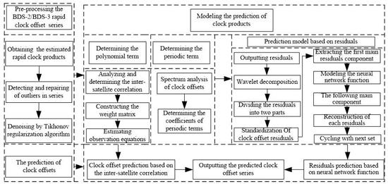
Figure 2 shows a detailed skeleton of the data processing strategy of the BDS-2/BDS-3 satellite clock offset prediction. The main steps include: (1) obtain BDS-2/BDS-3 rapid clock offset products and pre-process these data to improve the quality of the basic data series; (2) model the basic data series by a quadratic polynomial function; (3) model the remaining values of step (2) by some periodic functions; (4) further model the residuals of step (3) by PLS and the ANN algorithm; (5) predict the satellite clock offset series by using a combined model of (2), (3), and (4). In the ultra-rapid orbit estimation process, the predicted clock offsets are taken as the priori values with the corresponding constraints to improve the strength of the BDS orbit parameter estimation.

2.4. Optimal Arc Length Selection for the BDS Ultra-Rapid Predicted Orbit

It should be noted that the predicted part of the orbit is obtained by extrapolation from the observed part with the same initial state. According to published research, one-day observations cannot result in an optimal solution for the predicted part of the orbit. Thus, the length of the arc should be increased in the estimation of the initial orbit state. However, the model error will increase accordingly, with the arc length increasing through the combination of two adjacent observed orbits (rapid orbit of the previous day and ultra-rapid observed orbit of the current day). The optimal length of the observed arc for the predicted orbit in the initial orbit solution should be investigated as a priority for merging orbits shown in Figure 3. In this research, a strategy for the selection of an optimal arc length based on the Akaike information criterion (AIC) [40] is proposed. Moreover, the correlation between BDS-2 and BDS-3 is also considered in the estimation of the initial orbit state.

The AIC is closely related to an important concept in statistics—the Fisher likelihood theory. This theory was initially used to estimate Kullback–Leibler information. It is used to express the loss of one probability distribution or the relative values of information loss when using a model to represent data [41]. Assuming that the distribution of an observation’s uncertainty is normal, the value of AIC is defined by

$$\mathrm{AIC}=n\log ({\widehat{\sigma }}^2)+2k$$

(21)

where n is the number of the observations, k is the number of the parameters to be estimated, and $\widehat{\sigma }$ is the mean square error of the fitted residuals. On the right hand side of Equation (21), the first and second terms denote the fitting performance and complexity of the model, respectively [42]. An optimal model is the one that results in the minimum AIC value. In this study, Equation (21) is used to determine the optimal length of an arc in the estimation of the predicted initial orbit state.

To improve the accuracy of the initial orbit state, the high-precision information of BDS-3 satellites is also utilized in the orbit prediction by considering the inter-satellite correlation, which is similar to the method of the clock offset prediction in Section 2. The details of orbit prediction are described as follows.

Assume the orbit state at the i^th epoch is

$${\overrightarrow{X}}_{orb}(t_i)=\phi (t_i,t_0)\cdot {\overrightarrow{X}}_0$$

(22)

where ${\overrightarrow{X}}_0$ is the initial orbit state vector and φ(t,t₀) is the state transition matrix, which is based on the variational equations by the integrating with accelerations and coefficients of satellite orbit. φ(t,t₀) can be expressed as

$$\phi (t_i,t_0)=\left(\begin{array}{ccc}\frac{\partial r}{\partial r_0}& \frac{\partial r}{\partial {\dot{r}}_0}& \frac{\partial r}{\partial p}\\ \frac{\partial \dot{r}}{\partial r_0}& \frac{\partial \dot{r}}{\partial {\dot{r}}_0}& \frac{\partial \dot{r}}{\partial p}\\ \frac{\partial p}{\partial r_0}& \frac{\partial p}{\partial {\dot{r}}_0}& \frac{\partial p}{\partial p}\end{array}\right)=\left(\begin{array}{ccc}\frac{\partial r}{\partial r_0}& \frac{\partial r}{\partial {\dot{r}}_0}& \frac{\partial r}{\partial p}\\ \frac{\partial \dot{r}}{\partial r_0}& \frac{\partial \dot{r}}{\partial {\dot{r}}_0}& \frac{\partial \dot{r}}{\partial p}\\ & & I\end{array}\right).$$

(23)

In Equation (23), t₀ denotes the beginning epoch; r, $\stackrel{.}{\mathit{r}}$, p represents the positions, velocities and perturbations vectors, respectively, where the subscript of 0 denotes the corresponding initial states. I is an identity matrix. Equation (23) can be obtained by numerical integration method. Thus, the orbit fitting equations for estimating the initial state can be expressed as:

$$\{\begin{array}{l}{v}^{c_2}(t_i)={\phi }^{c_2}(t_i,t_0)\cdot {\overrightarrow{X}}_{{}_0}^{c_2}-{\overrightarrow{X}}_{{}_{orb}}^{c_2}(t_i)\\ v^{c_3}(t_i)={\phi }^{c_3}(t_i,t_0)\cdot {\overrightarrow{X}}_{{}_0}^{c_3}-{\overrightarrow{X}}_{{}_{orb}}^{c_3}(t_i)\end{array}$$

(24)

In Equation (24), C₂ and C₃ denote the BDS-2 and BDS-3 satellites, respectively; t_i and t₀ are the current and initial epochs respectively. It should be noted that ${\overrightarrow{X}}_{orb}$ consists of both ultra-rapid observed and the rapid orbits. The matrix form of Equation (24) can be expressed as

$$\mathit{V}(t_i)=\phi (t_i,t_0)\cdot {\overrightarrow{\mathit{X}}}_0-{\overrightarrow{\mathit{X}}}_{orb}(t_i)\mathit{P}(t_i).$$

(25)

Similarly, the weight matrix, P, in Equation (25) is similar to Equation (9), in which δ is the residual of the orbit fitting. Compared with traditional methods for the estimation of the initial orbit state, the BDS-2/BDS-3 combined solution using the inter-satellite correlation can improve the estimation of the parameters. However, the σ value in Equation (21) is calculated from Equation (24), and its determination should take the iteration process into consideration. The data processing strategy of BDS-2/BDS-3 ultra-rapid orbit prediction is shown in Figure 4.

3. Results

The ideas and methodologies proposed are tested using a one month (31 days, DOY 60-90, 2019) observations and rapid products. The main investigation includes a clock offset prediction model, an ultra-rapid orbit determination with the constraint of predicted clock offsets, and the optimal arc length of the initial state estimation for the predicted orbit.

3.1. BDS Satellite Clock Offset Prediction

In ultra-rapid orbit determination, the predicted clock offsets based on the rapid clock products of the previous day are taken as the constraints of clock parameters, so it is essential to acquire the predicted clock offsets precisely. In this study, the denoising method coupled with inter-satellite correlation and PLS is used to improve the accuracy of the predicted clock offset determination. Eight BDS-2 satellites and 19 BDS-3 satellites are used in the clock offset prediction, and the three schemes used for the test are:

Scheme 1: Based on the rapid clock offset products, a polynomial function plus periodic terms are selected in the clock offset prediction model, while the inter-satellite correlation and denoising algorithm are not considered.

Scheme 2: Similar to Scheme 1, the Tikhonov regularization algorithm and inter-satellite correlation are used in the prediction models.

Scheme 3: Similar to Scheme 2, the PLS method is added into the prediction solution to reduce the model residuals.

The rapid clock offset products in the three schemes are obtained from the rapid orbit determination, in which raw observations from the B1I and B3I signals are used to construct the undifferenced observation equations. The rapid clock offset is also taken as a reference for the accuracy assessment of the predicted clock offset series. Moreover, the two times difference method is adopted in the analyses of the clock offset accuracy. The accuracy is measured by the RMS of the differences between the predicted results and the reference. As an example, Figure 5 shows the daily accuracy (i.e., the RMS of all the epochs of a day) of the predicted clock offset obtained from the three schemes on DOY 60 for each of the BDS-2/BDS-3 satellites.

Table 2. The average daily accuracy of the clock offsets resulting from the three schemes and corresponding improvements.

Schemes	BDS-2 (ns)	Improvement	BDS-3 (ns)	Improvement
Scheme 1	3.16	-	2.68	-
Scheme 2	2.64	16.5%	2.17	19.0%
Scheme 3	1.88	40.5%	1.98	26.1%

lists the average daily accuracy of the clock offsets of all the satellites shown in Figure 5 for a period of 31 days, as well as the corresponding improvements.

These results indicate that: (1) compared with traditional approaches, the denoising method together with a consideration of inter-satellite correlation can improve accuracy up to 19.0%, which may be limited by unmodeled residuals. (2) Scheme 3 shows the best performance with an improvement in the prediction accuracy of 40.5% and 26.1% for the BDS-2 and BDS-3 satellites, respectively. The clock offset prediction of BDS-3 satellite is easier than that of BDS-2 satellite, because the frequency of the BDS-3 satellite clock is more stable than that of the BDS-2 satellite clock.

In addition, for an analysis of the model errors in the different schemes, the results of C14 and C21 on DOY 60 are selected as examples to represent BDS-2 and BDS-3 respectively, see Figure 6 for the residuals at each epoch (with a 5 min interval). It can be seen that Scheme 2 slightly improves the model results of Scheme 1, while Scheme 3 significantly improves the model results. The primary reasons for this result are that there are still many systemic variations in the residuals after modeling the clock offset via polynomial and periodic functions. The systemic character information of these residuals can be captured and modeled by PLS and the ANN algorithm. Therefore, the residuals of Scheme 3 are much smaller than those of Schemes 1 and 2.

To analyze the inter-satellite correlation, the correlation coefficients among all BDS satellites are calculated and listed in

Table 3. Correlation coefficients (average) between different satellites over one day (DOY 60, 2019).

Satellite Types	BDS-2	BDS-3
BDS-2	0.52	0.64
BDS-3	0.64	0.49

. As shown in Table 3, the correlation values are between 0.49 and 0.64 (absolute values), which are well above the minimum recommended level of significance (i.e., 0.50). It also is indicated that the inter-satellite correlation of BDS-2 and BDS-3 is stronger than that of BDS-2 and BDS-3. The inter-satellite correlation information can be used to improve the accuracy of the clock offset estimation/prediction for BDS-2 due to the high-quality nature of the BDS-3 satellite clocks. For example, BDS-2 can benefit from the combined estimation process.

Moreover, to analyze the differences between the model results obtained from the proposed approaches (Scheme 3 and Scheme 2) and the traditional method (Scheme 1), the histograms for C14 and C21 and the above three schemes during a 31 day period are shown in Figure 7. It is suggested that Scheme 3 can not only significantly improve the clock offset prediction and but also reduce the model’s residuals.

3.2. Ultra-Rapid Orbit Determination Based on Clock Offsets Constraint

To verify the proposed strategy (the precision of ultra-rapid orbit determination with the aid of precise satellite clock offsets can be improved), a number of real BDS-2/BDS-3 data were collected and tested. The distribution of the selected stations for our experiments is shown in Figure 8, which consists of 18 international GNSS Monitoring and Assessment Service (iGMAS) stations and 9 Multi-GNSS EXperiment (MGEX) stations, as well as the B1I and B3I signals of BDS-3 satellites. In orbit determination, un-differenced ionosphere-free code and a phase combination of B1I and B3I observations were conducted. Moreover, the arc length is set to three-days, and a parameter configuration similar to [10,13] is used. It is noted that the un-differenced and double-differenced methods are two popular data processing strategies for orbit determination, and they each have their own advantages and disadvantages. For example, the satellite clock offset parameters will be removed and the data processing be simplified in a double-differenced mode (e.g., Bernese software). This is beneficial to orbit determination if the satellite clock parameters cannot be precisely known. However, the correlation information of the satellite clock parameters is lost, because they are considered unrelated in a double-differenced mode. In contrast, the satellite clock offset parameters are modeled and estimated together with orbit parameters in the un-differenced mode (e.g., PANDA software). This mode is helpful for orbit determination if the satellite clock parameters can be accurately obtained. Otherwise, it will lead to a decrease in orbit determination precision if the precision of satellite clock parameters is poor. Thus, un-differenced and double-differenced modes are equivalent if satellite clock parameters can be precisely known and are temporally unrelated. The four test scenarios are designed as follows:

Scenario 1: The broadcast clock information from navigation files is used in the orbit determination of BDS-3 (B1I and B3I observations), in which a 5000 m accuracy of the clock offset is utilized as a constraint.

Scenario 2: The rapid precise clock products from the WHU Analysis Centre are used in the orbit determination of BDS3 (B1I and B3I observations), in which 10 m is utilized as a constraint.

Scenario 3: The new signals (B1C and B2a) are used, and the broadcast clocks from navigation files are used in the orbit determination, in which a 5000 m accuracy of the clock error is used as a constraint.

Scenario 4: The new signals (B1C and B2a) are used, and the rapid precise clock products from the WHU Analysis Centre are used for the orbit determination, in which a 10 m accuracy of the clock error is used as a constraint.

In the experiment, the constraint of the clock offset parameter is taken as a condition equation to estimate the orbit determination parameter. In this study, the clock accuracies of the precise clock and broadcast clock are set as 10 m and 5000 m, respectively, which are referenced in [8,13]. Similarly, experiments using 31 days (DOY 30–60, 2019) of data are conducted for the analyses of the orbit results estimated from the use of the constraints on the clock parameters. The final products from the WHU Analysis Centre are used as references for the validation of the test results. The results of C14 and C21 are chosen as examples for the differences between Scenario 1 and Scenario 2. Figure 9 shows their daily accuracy, from which it can be seen that Scenario 2 (red) is slightly better on most days than Scenario 1 (black) for the two types of satellites. In Figure 9, the orbit determination results of C21 in DOY 71, 2019 were blank due to C21’s orbit maneuver during this day, which lead to a solution divergence.

Figure 10 shows the orbit accuracy for all satellites (distinguished with BDS-2 and BDS-3 satellites) on DOY 60.

Table 4. The average daily accuracy of the BDS rapid orbit resulting from two types of clocks and the corresponding improvements.

Type of Clock	BDS-2 (cm)	Improvement	BDS-3 (cm)	Improvement
Broadcast	12.52	-	13.68	-
Precise	11.68	6.7%	13.19	3.6%

lists the average daily accuracy of the BDS-2 and BDS-3 orbits resulting from Scenario 1 and Scenario 2, respectively, of all the satellites shown in Figure 10, for all 31 days, and their corresponding improvements. One can see that the orbit obtained from the precise clocks is slightly better than that from the broadcast clocks (6.7% and 3.6% for BDS-2 and BDS-3, respectively).

The clock offsets are also analyzed using the two times difference (referred to as the WHU final products). The change in the accuracy of the clock offset is indicated fby the statistical results of Scenario 1 and Scenario 2 shown in Figure 11 and

Table 5. The average daily accuracy of the BDS rapid clock offsets resulting from the two types of clocks and the corresponding improvement.

Type of Clock	BDS-2 (ns)	Improvement	BDS-3 (ns)	Improvement
Broadcast	0.95		0.88
Precise	0.49	48.4%	0.77	12.5%

, as Figure 9 and Figure 10, and Table 4, respectively. From the average daily accuracy of all the satellites and the 31 days, one can see that the accuracy improvements of the BDS-2 and BDS-3 satellites are 48.4% and 12.5%, respectively.

For Scenarios 3 and 4, due to the availability of limited numbers of stations for B1C and B2a observations during the period of the experiments (only iGMAS stations had BDS-3 observations, but with low integrity), and the BDS-2 orbit results were omitted in the WHU products. Figure 12 shows the BDS-3 orbit accuracy for two days (DOYs 67 and 78), as examples for a comparison of the accuracy differences of the two test scenarios. One can see that Scenario 4 (precise clocks with constraint conditions) outperforms Scenario 3 (a broadcast clock), which is consistent with the previous conclusions from Scenarios 1 and 2. However, the accuracy (1D RMS) of the new signals’ orbit is poorer than 40 cm, which is significantly lower than the ones from the B1I and B3I observations.

For the BDS-2/BDS-3 combined ultra-rapid orbit determination, the predicted clock offsets based on the rapid clock products are also assessed using 31 days of experimental data. In the orbit determination, the same observations as the rapid orbit determination solutions are selected, in which the arc length of the observations is reduced to one day. The procedure is the same as above. The broadcast and the predicted clock offsets, along with the constraints on the clock parameters of 5000 m and 10 m, respectively, are input into the ultra-rapid orbit determination. The results of DOY 60, selected as the examples, are shown in Figure 13 and Figure 14 to show the differences resulting from the two different strategies.

Table 6. The average daily accuracy of the ultra-rapid orbit resulting from two types of clocks and the corresponding improvement.

Type of Clock	BDS-2 (cm)	Improvement	BDS-3 (cm)	Improvement
Broadcast	32.6	-	28.8	-
Precise	29.6	9.2%	27.4	5.0%

and

Table 7. The daily average accuracy of the ultra-rapid clocks resulting from two types of clocks and the corresponding improvement.

Type of Clock	BDS-2 (ns)	Improvement	BDS-3 (ns)	Improvement
Broadcast	0.83	-	1.02	-
Precise	0.81	2.4%	1.04	2.0%

show the average daily accuracy of the BDS-2 and BDS-3 orbits and clock offsets, respectively, of all the satellites for 31 days, shown in Figure 13 and Figure 14, respectively, and the corresponding improvements.

From the above results, it can be concluded that the use of constraints on the clock parameters can improve the accuracy of the orbit and clock of the BDS products. However, due to the limited accuracy of the predicted clock offsets, the improvements of the clock products are under 10%. This result needs to be further investigated using more observations and more accurate rapid clock products.

3.3. The Ultra-Rapid Predicted Orbit from Improved Models

In this section, experimental results for the improved model of BDS ultra-rapid prediction are verified. The AIC values and the inter-satellite correlation are considered in the estimation of the initial orbit state. In the experiments, the predicted ultra-rapid orbits of the BDS-2/BDS-3 satellites for 21 days are output with a one day arc length. It is noted that the rapid orbit of the previous day for each of the experimental solutions needs to be prepared before an ultra-rapid orbit determination is performed. In the accuracy analysis of the predicted orbit, again, the final products from the WHU Analysis Centre are also used as the references for the validation of the experimental results.

First, the feasibility of the AIC values is tested with simulation experiments. To explain the relationship between the AIC value and its corresponding predicted orbit accuracy, the average of the daily RMS for all BDS satellites and the corresponding AIC value from DOY 60 are taken as an example. Figure 15a shows the orbit accuracy variation with the AIC value, where 24 data samples selected are shown for the DOY. The accuracy of the predicted orbit (1D RMS) presents a high-correlation with the AIC value, which is consistent with the results of the C21 and C14 satellites orbits shown in Figure 15b.

Figure 16 shows the C14 and C21 results for a period of 21 days, in which two days of results (between 79 and 80) are excluded because of their lower accuracy. This figure indicates that the accuracy of the predicted orbit has been significantly improved based on the AIC selection model in the estimation of the initial state of the BDS’s predicted orbit.

Based on the ultra-rapid orbit determination, the observed part is estimated by imposing constraints on the clock parameters, i.e., the clock offsets obtained from the solution of high-precision prediction are treated as constraints in the estimation of the orbit’s initial state for the observed part. Moreover, the observed part will be taken as the observations in estimating the orbit’s initial state for the predicted part. Identically, the 21 day predicted orbits are compared against the final products provided from the WHU Analysis Centre. For more details, the accuracy of the original predicted orbit (the initial state is estimated from a one day observed ultra-rapid orbit), the AIC selected orbit (minimum of the AIC values), and the sub-optimal selected orbit (before and after the minimum of AIC values) are presented in

Table 8. Accuracy of the BDS’ predicted orbit and improvement.

Schemes	BDS Orbit (cm)	Improvement
Original	349	-
Before three hours	71	79.6%
Before two hours	66	81.1%
Before one hour	63	81.9%
Minimum	62	82.2%
After one hour	62	82.2%
After two hours	63	81.9%
After three hours	63	81.9%

.

It can be found that the accuracy of the BDS predicted orbits is significantly improved after considering the rapid orbit in the estimation of the initial orbit state. The optimal arc length can be determined by the selection of the AIC values, from which the improvement can reach 82.2%, compared with the original predicted orbit. However, the accuracy of the BDS predicted orbit is still worse than 60 cm, which may be further improved by the use of some more accurate perturbation models, attitude models, etc.

4. Discussion

In this paper, to improve the accuracy of BDS-2/BDS-3 combined ultra-rapid orbit products, the predicted clock offsets based on the rapid clock products of the previous day are taken as constraints of clock parameters in ultra-rapid orbit determination. According to the prediction strategy, the Tikhonov regularization algorithm, inter-satellite correlation, and the PLS methods are considered to optimize the prediction model. Compared with traditional approaches, the denoising method together with consideration of inter-satellite correlation can improve accuracy up to 19.0%, which may be limited by unmodeled residuals. Due to the more stable frequency of the satellites’ onboard clocks, the accuracy of BDS-3 is better than that of BDS-2. Based on the BDS-2/BDS-3 satellites’ combined rapid orbit determination, four further scenarios for testing various frequencies and clock offset products are selected. From the average daily accuracy of all the satellites with 31 days, one can see that the accuracy improvements of the BDS-2 and BDS-3 satellites are 48.4% and 12.5%, respectively. Moreover, the accuracy (1D RMS) of the new signals’ orbit is poorer than 40 cm, which is significantly lower than the ones from B1I and B3I observations. However, due to the limited accuracy of the predicted clock offsets, the improvements of the clock products are under 10%, which needs to be further investigated using more observations and more accurate rapid clock products.

For the predicted part of the ultra-rapid orbit, it is indicated that one-day arc length of the observations could not result in optimal results for the initial orbit states. Thus, the rapid orbit obtained from the previous day is used as observations in the observed part of the ultra-rapid orbit to estimate the orbit’s initial states. Moreover, to select the optimal length of the arc, the AIC values are proposed to be used in the new strategy. The AIC values and the inter-satellite correlation are considered in the estimation of the orbit’s initial state. The accuracy of the predicted orbit (1D RMS) presents a high-correlation with the AIC value, which is consistent with the results of the C21 and C14 satellites orbits shown in Figure 15b. This result indicates that the accuracy of the predicted orbit has been significantly improved based on the AIC selection model in the estimation of the initial state of the predicted BDS orbit.

It is noted that the orbit accuracies that resulted from the improved models are still not as desirable as they should be (i.e., worse than 27 cm and 60 cm for the observed and predicted orbit parts, respectively). Future work will focus on the following investigations: (1) the accuracy of the predicted clock offsets may be improved by rapid clock products and predicted models; (2) models such as perturbation models and attitude models of BDS satellites may need to be refined with larger data sets; (3) highly precise BDS-3 satellite information needs to be further exploited to determine the best use.

5. Conclusions

GNSS satellite ultra-rapid orbits play a critical role in the performance of GNSS services, especially for Chinese BDS due to its limited number of observations and the uneven distribution of the tracking stations. It is challenging to achieve the same accuracy as GPS. In this research, new approaches for better orbit solutions are proposed to improve BDS ultra-rapid products.

First, to improve the accuracy of the parameter estimates in ultra-rapid orbit determination, the BDS-predicted clock offsets are used as constraints. The traditional clock prediction models are then modified for an improved prediction of the BDS-2/BDS-3 combined clock offsets. The Tikhonov regularization based denoising method inter-satellite correlation, and the PLS method are investigated to improve the accuracy of the predicted BDS-2/BDS-3 combined clock offset. Compared with the traditional method, our results show that the improvements to the predicted clock offsets are 40.5% and 26.1% for the BDS-2 and BDS-3 satellites, respectively.

Second, experimental results for the constraints imposed on clock parameters in orbit determination have showed that: Rapid orbit accuracy is improved with 6.7% and 3.6% for BDS-2 and BDS-3 satellites, respectively, and the improvements to the clock offsets can be up to 48.4% and 12.5%, respectively. Moreover, by using a constraint on the predicted clock offsets, the observed BDS-2 and BDS-3 ultra-rapid orbits were improved 9.2% and 5.0%, respectively, while their clock offsets were improved by 2.4% and 2.0%. In general, minor improvements to the ultra-rapid observed orbit were made by using the constraints of the predicted BDS-2/BDS-3 satellites’ clock offsets.

The experimental results showed that the AIC values presented a high correlation with the accuracy of the predicted orbit. Moreover, the AIC selection strategy significantly improved the accuracy of the predicted orbit, compared with the traditional method. When the clock offset constraints were applied in ultra-rapid orbit determination and the use of the AIC value selection method, the BDS’s predicted orbits were improved by 82.2%, compared to the traditional strategy. These results suggest that the improved models can enhance BDS-2/BDS-3 combined satellites’ ultra-rapid orbit products.

References

- CSNPC. China Satellite Navigation Project Center. Compass/Beidou Navigation Satellite System Development; CSNPC: Beijing, China, 2009. [Google Scholar]
- Yang, Y.; Li, J.; Wang, A.; Xu, J.; He, H.; Guo, H. Preliminary assessment of the navigation and positioning performance of BeiDou regional navigation satellite system. Sci. China Earth Sci. 2014, 57, 144–152. [Google Scholar] [CrossRef]
- BeiDou Satellite Launch List. Available online: http://www.beidou.gov.cn/ (accessed on 1 May 2018).
- Yang, Y.X. Performance Analysis of BDS-3 Demonstration System. In Proceedings of the ISGNSS, Hong Kong, China, 10–13 December 2017. [Google Scholar]
- Yang, Y.X.; Li, J.L.; Xu, J.Y.; Tang, J.; Guo, H.R.; He, H.B. Contribution of the Compass satellite navigation system to global PNT users. Chin. Sci. Bull. 2011, 56, 2813. [Google Scholar] [CrossRef]
- Zhao, Q.; Wang, C.; Guo, J.; Wang, B.; Liu, J. Precise orbit and clock determination for BeiDou-3 experimental satellites with yaw attitude analysis. GPS Solut. 2017, 22, 4. [Google Scholar] [CrossRef] [Green Version]
- Zhou, S.; Hu, X.; Wu, B.; Liu, L.; Qu, W.; Guo, R.; He, F.; Cao, Y.; Wu, X.; Zhu, L.; et al. Orbit Determination and Time Synchronization for a GEO/IGSO Satellite Navigation Constellation with Regional Tracking Network. Sci. China Phys. Mech. Astron. 2011, 54, 1089–1097. [Google Scholar] [CrossRef]
- Guo, J. The Impacts of Attitude, Solar Radiation and Function Model on Precise Orbit Determination for GNSS Satellites; Wuhan University: Wuhan, China, 2014. [Google Scholar]
- Dilssner, F.; Springer, T.; Schönemann, E. Estimation of satellite antenna phase center corrections for BeiDou. In Proceedings of the IGS Workshop, Pasadena, CA, USA, 23–27 June 2014. [Google Scholar]
- Tan, B.; Yuan, Y.; Wen, M.; Ning, Y.; Liu, X. Initial Results of the Precise Orbit Determination for the New-Generation BeiDou Satellites (BeiDou-3) Based on the iGMAS Network. ISPRS Int. J. Geo Inf. 2016, 5, 196. [Google Scholar] [CrossRef]
- Ge, M.R.; Zhang, H.P.; Jia, X.L.; Song, S.L.; Wickert, J. What is achievable with the current compass constellation? In Proceedings of the 25th International Technical Meeting of The Satellite Division of the Institute of Navigation (ION GNSS 2012), Nashville, TN, USA, 17–21 September 2012; pp. 331–339. [Google Scholar]
- Montenbruck, O.; Hauschild, A.; Steigenberger, P.; Hugentobler, U.; Teunissen, P.; Nakamura, S. Initial assessment of the COMPASS/BeiDou-2 regional navigation satellite system. GPS Solut. 2013, 17, 211–222. [Google Scholar] [CrossRef]
- Hu, C.; Wang, Q.; Wang, Z.; Moraleda, A. New-Generation BeiDou (BDS-3) Experimental Satellite Precise Orbit Determination with an Improved Cycle-Slip Detection and Repair Algorithm. Sensors 2018, 18, 1402. [Google Scholar] [CrossRef]
- Chen, J.; Hu, X.; Tang, C.; Zhou, S.; Guo, R. Orbit determination and time synchronization for new-generation Beidou satellites: Preliminary results. Sci. Sin. Phys. Mech. Astron. 2016, 46, 119502. [Google Scholar] [CrossRef] [Green Version]
- Zhang, X.; Wu, M.; Liu, W.; Li, X.X.; Yu, S.; Lu, C.; Wickert, J. Initial assessment of the COMPASS/BeiDou-3: New-Generation navigation signals. J. Geod. 2017, 91, 1225–1240. [Google Scholar] [CrossRef]
- Ren, X.; Yang, Y.; Zhu, J.; Xu, T. Orbit Determination of the Next-Generation Beidou Satellites with Intersatellite Link Measurements and a Priori Orbit Constraints. Adv. Space Res. 2017, 60, 2155–2165. [Google Scholar] [CrossRef]
- Yang, D.; Yang, J.; Li, G.; Zhou, Y.; Tang, C.P. Globalization highlight: Orbit determination using BeiDou inter-satellite ranging measurements. GPS Solut. 2017, 21, 1395–1404. [Google Scholar] [CrossRef]
- Tang, C.P.; Hu, X.G.; Zhou, S.S.; Guo, R.; He, F.; Liu, L.; Zhu, L.F.; Li, X.J.; Wu, S.; Zhao, G. Improvement of orbit determination accuracy for Beidou Navigation Satellite System with Two-way Satellite Time Frequency Transfer. Adv. Space Res. 2016, 58, 1390–1400. [Google Scholar] [CrossRef]
- Li, X.X.; Yuan, Y.Q.; Zhu, Y.T.; Huang, J.D.; Wu, J.Q.; Xiong, Y.; Zhang, X.H.; Li, X. Precise orbit determination for BDS3 experimental satellites using iGMAS and MGEX tracking networks. J. Geod. 2019, 93, 103–117. [Google Scholar] [CrossRef]
- Teunissen, P.; Joosten, P.; Odijk, D. The Reliability of GPS Ambiguity Resolution. GPS Solut. 1999, 2, 63–69. [Google Scholar] [CrossRef] [Green Version]
- Li, X.X.; Ge, M.R.; Douša, J.; Wickert, J. Real-time precise point positioning regional augmentation for large GPS reference networks. GPS Solut. 2014, 18, 61–71. [Google Scholar] [CrossRef]
- Wang, Q.; Hu, C.; Mao, Y. Correction Method for the Observed Global Navigation Satellite System Ultra-Rapid Orbit Based on Dilution of Precision Values. Sensors 2018, 18, 3900. [Google Scholar] [CrossRef] [PubMed]
- Qing, Y.; Lou, Y.; Dai, X.; Liu, Y. Benefits of satellite clock modeling in BDS and Galileo orbit determination. Adv. Space Res. 2017, 60, 2550–2560. [Google Scholar] [CrossRef]
- Huang, G.; Zhang, Q. Real-time estimation of satellite clock offset using adaptively robust Kalman filter with classified adaptive factors. GPS Solut. 2012, 16, 531–539. [Google Scholar] [CrossRef]
- Guo, H.; Yang, Y. Analyses of Main Error Sources on Time-Domain Frequency Stability for Atomic Clocks of Navigation Satellites. Geomat. Inf. Sci. Wuhan Univ. 2009, 34, 218–221. [Google Scholar]
- Strandjord, K.; Axelrad, P. Improved prediction of GPS satellite clock sub-daily variations based on daily repeat. GPS Solut. 2018, 22, 58. [Google Scholar] [CrossRef]
- Huang, G.; Cui, B.; Zhang, Q.; Fu, W. An Improved Predicted Model for BDS Ultra-Rapid Satellite Clock Offsets. Remote Sens. 2018, 10, 60. [Google Scholar] [CrossRef]
- Senior, K.; Coleman, M. The next generation GPS time. Navigation 2017, 64, 411–426. [Google Scholar] [CrossRef]
- Davis, J.; Bhattarai, S.; Ziebart, M. Development of a Kalman filter based GPS satellite clock time-offset prediction algorithm. In Proceedings of the European Frequency Time Forum (EFTF), Gothenburg, Sweden, 23–27 April 2012. [Google Scholar] [CrossRef]
- Wang, Y.; Lv, Z.; Qu, Y.; Li, L.; Wang, N. Improving prediction performance of GPS satellite clock bias based on wavelet neural network. GPS Solut. 2017, 21, 523–534. [Google Scholar] [CrossRef]
- Huang, G.; Zhang, Q.; Xu, G. Real-time clock offset prediction with an improved model. GPS Solut. 2014, 18, 95–104. [Google Scholar] [CrossRef]
- Mao, Y.; Wang, Q.X.; Hu, C.; Yang, H.Y.; Yang, X.; Yu, W.X. New clock offset prediction method for BeiDou satellites based on inter-satellite correlation. Acta Geod. Geophys. 2019, 54, 35–54. [Google Scholar] [CrossRef]
- Choi, K.; Ray, J.; Griffiths, J.; Bae, T. Evaluation of GPS orbit prediction strategies for the IGS Ultra-rapid products. GPS Solut. 2013, 17, 403–412. [Google Scholar] [CrossRef]
- Li, Y.; Gao, Y.; Li, B. An impact analysis of arc length on orbit prediction and clock estimation for PPP ambiguity resolution. GPS Solut. 2015, 19, 201–213. [Google Scholar] [CrossRef]
- Stacey, P.; Ziebart, M. Long-term extended ephemeris prediction for mobile devices. In Proceedings of the International Technical Meeting of the Satellite Division of the Institute of Navigation, Portland, OR, USA, 20–23 September 2011; Volume 28, pp. 3235–3244. [Google Scholar]
- Wang, Q.; Hu, C.; Chang, G. Impacts of Earth rotation parameters on GNSS ultra-rapid orbit prediction: Derivation and real-time correction. Adv. Space Res. 2017, 60, 2855–2870. [Google Scholar] [CrossRef]
- Chang, G.; Chen, C.; Yang, Y.; Xu, T. Tikhonov regularization based modeling and sidereal filtering mitigation of GNSS multipath errors. Remote Sens. 2018, 10, 1801. [Google Scholar] [CrossRef]
- Hu, C.; Wang, Q.; Mao, Y. An improved model for BDS satellite ultra-rapid clock offset prediction based on BDS-2 and BDS-3 combined estimation. Acta Geod. Geophys. 2019. under review. [Google Scholar]
- Mao, Y.; Wang, Q.; Hu, C. Characteristic analysis of BDS-3 satellite onboard clock. Geomat. Inf. Sci. Wuhan Univ. 2018. [Google Scholar]
- Akaike, H. Likelihood of a model and information criteria. J. Econom. 1981, 16, 3–14. [Google Scholar] [CrossRef]
- Cover, T.; Thomas, J. Elements of Information Theory; John wiley & Sons: New York, NY, USA, 2012. [Google Scholar]
- Burnham, K.; Anderson, D. Multimodel inference: Understanding AIC and BIC in model selection. Soc. Methods Res. 2004, 33, 261–304. [Google Scholar] [CrossRef]
Figure 1.
Frequency analysis of eight BeiDou demonstration system (BDS) satellites (black arrow is period term beyond one day; red arrow is the significant periodic terms in one day).
Figure 2.
Flowchart for the procure of clock offset prediction.
Figure 3.
Merger of the two-day observed orbit for the estimation of the orbit’s initial states.
Figure 4.
Improved model of the initial orbit state for the predicted orbit.
Figure 5.
Daily accuracy of the clock offsets of BDS-2 (left) and BDS-3 (right) obtained from three schemes on DOY 60.
Figure 6.
Residuals of each epoch on DOY 60 across the three schemes tested.
Figure 7.
Histogram of the residuals of the C14 and C21 satellites resulting from three schemes during the period of 31 days.
Figure 8.
Distribution of selected stations for both ultra-rapid and rapid orbit determination. MGEX, Multi-GNSS Experiment; iGMAS, international GNSS Monitoring and Assessment Service.
Figure 9.
Daily orbit accuracy comparison of the two satellites (C14 and C21) resulting from Scenario 1 (black) and Scenario 2 (red) during the 31 day period.
Figure 10.
Daily orbit accuracy of each satellite (BDS-2: left, BDS-3: right) resulting from Scenario 1 (black) and Scenario 2 (red) on DOY 60.
Figure 11.
The daily clock offset accuracy of various satellites resulting from Scenario 1 (black) and Scenario 2 (red) and the B1I and B3I observations during the 31 day period (upper panels) and on DOY 60 (bottom panels).
Figure 12.
The daily accuracy of the BDS-2/BDS-3 rapid orbit of each satellite obtained from two types of clock offsets, and from the B1C and B2a observations, on DOYs 67 (left) and 78 (right).
Figure 13.
The daily accuracy of the ultra-rapid observed orbit of each satellite obtained from the broadcast and predicted clocks on DOY 60.
Figure 14.
The daily accuracy of the clock offset of each satellite estimated from the broadcast and predicted clocks on DOY 60.
Figure 15.
AIC values and the corresponding BDS orbit accuracies on DOY 60.
Figure 16.
Accuracy of the BDS’s predicted orbit for 21 days from satellites C14 (left) and C21 (right).