Urban Landscape Change Analysis Using Local Climate Zones and Object-Based Classification in the Salt Lake Metro Region, Utah, USA

Abstract

Urban areas globally are vulnerable to warming climate trends exacerbated by their growing populations and heat island effects. The Local Climate Zone (LCZ) typology has become a popular framework for characterizing urban microclimates in different regions using various classification methods, including a widely adopted pixel-based protocol by the World Urban Database and Access Portal Tools (WUDAPT) Project. However, few studies to date have explored the potential of object-based image analysis (OBIA) to facilitate classification of LCZs given their inherent complexity, and few studies have further used the LCZ framework to analyze land cover changes in urban areas over time. This study classified LCZs in the Salt Lake Metro Region, Utah, USA for 1993 and 2017 using a supervised object-based analysis of Landsat satellite imagery and assessed their change during this time frame. The overall accuracy, measured for the most recent classification period (2017), was equal to 64% across 12 LCZs, with most of the error resulting from similarities among highly developed LCZs and non-developed classes with sparse or low-stature vegetation. The observed 1993–2017 changes in LCZs indicated a regional tendency towards primarily suburban, open low-rise development, and large low-rise and paved classes. However, despite the potential for local cooling with landscape transitions likely to increase vegetation cover and irrigation compared to pre-development conditions, summer averages of Landsat-derived top-of-atmosphere brightness temperatures showed a pronounced warming between 1992–1994 and 2016–2018 across the study region, with a 0.1–2.9 °C increase among individual LCZs. Our results indicate that future applications of LCZs towards urban change analyses should develop a stronger understanding of LCZ microclimate sensitivity to changes in size and configuration of urban neighborhoods and regions. Furthermore, while OBIA is promising for capturing the heterogeneous and multi-scale nature of LCZs, its applications could be strengthened by adopting more generalizable approaches for LCZ-relevant segmentation and validation, and by incorporating active remote sensing data to account for the 3D complexity of urban areas.

1. Introduction

Worldwide expansion and warming of urban regions present an important concern for the well-being of their residents, creating an urgent need for cost-effective strategies to track changing microclimates and inform current and future planning [1,2,3,4]. Previous research has extensively focused on urban heat island (UHI) phenomena manifested in significantly higher temperatures of cities compared to their surroundings due to unique thermal properties of urban land cover/use (LULC), building materials, human activities and other factors [5,6,7,8,9]. Increases in both ambient urban temperatures and frequency of extreme heat events [10] pose major threats to human health, especially in areas with higher population densities and vulnerable social and demographic groups [1,2,11]. These concerns become even more apparent considering that by 2050, 66% of the world’s population is projected to be urban, while 82% of the North American population already lives in urban areas [12]. However, as UHIs are frequently analyzed at metropolitan scales [8,13,14], it remains less well known how specific local urbanization patterns contribute to their intensity and persistence in regions with ongoing development [15,16].

Adapting urban policy and planning to these novel thermal risks thus requires a more explicit understanding of the distribution and dynamics of urban microclimates [17,18,19], which cannot be adequately represented by the rural-urban temperature differences or traditional LULC types alone [6,20,21]. To better represent landscape drivers of UHIs, Stewart and Oke (2012) proposed the classification of Local Climate Zones (LCZs) as urban regions with similar surface cover (Figure A1, Appendix), building materials, configuration and types of human activities [6]. There are 17 total classes, where LCZs 1–6 are built-up types with different building compactness and height, types 7–10 represent other urban-specific surfaces and land uses, and types A–G are non-built land cover types that are not unique to cities [6,21]. The distinctions among LCZs are defined by measurable physical properties (see the Appendix in [6]), and thus each class has a somewhat unique microclimate, as supported by both in situ observations and numeric modeling [22,23,24,25]. As such, the LCZ framework enables objective, standardized comparisons of urbanization patterns from a climate impact perspective [6,9,21], as well as other applications in climate modeling [20] and landscape design [17]. The LCZs also appeal to planning and policy [26,27,28,29] because operationalizing the new insights from UHI studies requires framing them in the lexicon of design and planning, which often relies on discrete concepts such as zoning boundaries, building dimensions, and similar. Measurements of urban climates, on the other hand, are frequently scale-sensitive and continuous in space and time. The LCZ framework aims to reconcile this discrepancy by summarizing micro- and meso-climatic variation across the landscape and packaging this information into discrete zones that can be translated into specific measurable parameters of the urban environments [6,26,28,30,31,32].

Recognizing this potential, multiple efforts have started to map LCZs in different cities across the world [9,21,26,33,34,35], as discussed in more detail in the next section; however, relatively few studies have applied this framework in the context of urban change [36,37]. The potential of urban temperatures and UHIs to continue increasing with ongoing development implies that urban neighborhoods in growing cities may experience future warming, even without substantial change in their landscape morphology and structure [13,37]. Thus, understanding the dynamics of urban LCZs and their relationship to microclimatic transformation represents an important research need, which could be addressed using existing and new spatially comprehensive and temporally rich satellite products. For instance, more than 30 years of openly accessible Landsat imagery provides an unprecedented opportunity to characterize LCZs and their change in different urban regions experiencing transitions of their LULC and population [38,39]. Our study presents a case for such analysis by using an object-based image analysis (OBIA) workflow to classify LCZs in the Salt Lake City Metro Region, USA from 30 m Landsat imagery and assess their shift with the ongoing urbanization from 1993 to 2017. We subsequently discuss the strengths and challenges in applying OBIA towards LCZ classification from medium-resolution imagery, reflect on the potential of LCZs to characterize long-term urban transformation and outline key future research needs and potential directions.

2. Background

2.1. Background on LCZ Applications and Alternative Mapping Methodologies

Efforts to map LCZs to date have highlighted many useful insights and methodological opportunities for applying LCZs towards urban change analyses [34,40,41]. Typically, LCZ mapping relies on supervised image classification workflows, where training samples of LCZs are generated from known locations by expert selection and are subsequently used to train statistical algorithms to recognize LCZs in the unmapped areas [21,32]. One particularly well-known protocol was developed by the World Urban Database and Access Portal Tools (WUDAPT) project [20,21,31], a community-based initiative aiming to develop a global database representing urban form and function in a format applicable to climate-relevant research and modeling. The WUDAPT level 0 LCZ classification approach [21] uses publicly available Landsat satellite imagery resampled from 30-m spatial resolution to ~100–150 m. The training sample and validation regions for each LCZ are selected using expert knowledge and cost-effective platforms such as Google Earth software, and then a Random Forest classifier is used to map LCZs in the open source software, SAGA. Among different studies, notable recent outcomes of WUDAPT include a comparison of surface urban heat islands across 50 global cities [33] and a continental-scale LCZ map for Europe [9].

While Landsat imagery has been a prevailing input to LCZ mapping to date [20,21,42,43,44,45], other datasets have also been used recently as either primary inputs or supplementary to Landsat. An analysis of LCZs and UHIs in Beirut [46] used a Sentinel-2 image together with three Landsat-8 scenes in a multi-date classification input, which facilitated the differentiation of vegetation types based on Sentinel-2′s red edge band. Similarly, an assessment of the effect of input data on LCZ mapping focusing on nine cities in Europe recommended a joint use of Landsat-8 and Sentinel-2 [47]. Another study focusing on Milan, Italy [48] compared LCZ maps derived from Landsat-8, Sentinel-2 and 5-m RapidEye satellite imagery, where the latter input resulted in ~4–10% lower overall accuracy than two others. Alternatively, an effort to map LCZs in three metropolitan areas in Texas, USA [28] combined the existing 30-m National Land Cover Dataset (NLCD) raster product and airborne LiDAR datasets to discriminate LCZs via a multi-step decision-making algorithm based on both horizontal identity and 3-dimensional structure of land cover. Another notable example of using active remote sensing in LCZ mapping involved the application of Sentinel-1 synthetic aperture radar (SAR) imagery in 29 global cities [49], which suggested the importance of using local statistical features relevant to urban heterogeneity in classification success.

However, despite efforts to increase the informative richness of input data and common use of sophisticated machine-learning algorithms, classification accuracy among these previous studies highly varied, ranging from greater than 81% [21,43,44,45] to less than 70% [35,42,46,49]. One of the potential key reasons behind this could be the availability and quality of training samples, as suggested by the LCZ transferability analysis in [50] which highlighted the importance of city or local ecoregion-specific training data for such transferability and the potential need to strategically combine training data from different cities in broader-scale regional mapping. Another potentially important factor could lie in the pixel-based nature of LCZ classifications and spatial resolution of the input data. In some cases, individual pixels may be too small to capture the relevant mixtures of cover types (i.e., paved surfaces, vegetation, buildings), or, in contrast, too large to adequately capture the contrasts between LCZs with similar mixtures of different urban surfaces. These issues may be magnified in historical neighborhoods of older cities with irregular, complex patterns making it difficult to identify LCZ boundaries [51]. Collectively, these challenges imply that spatial scales that best represent individual LCZs may vary among different urban regions and even among the individual LCZs themselves, which makes it difficult to optimize accuracy under one standard mapping unit size [43,52].

Recognizing this challenge, studies have proposed different modifications to mapping units and/or classification workflow. For instance, LCZ analysis in Wuhan, China, found 500m to be a more optimal spatial resolution for investigating the relationships between landscape pattern and temperature [52]. This result was consistent with the originally proposed LCZ dimensions, namely the minimum diameter of 400–1000 m to account for thermal continuity and broad-scale atmospheric effects [6]. Alternatively, a study mapping LCZs in Kyiv, Ukraine [35] retained some of the spectral variation at the Landsat 30 m resolution by calculating additional statistics (e.g., mean and extrema of spectral values) when resampling to 120 m. This adjustment, however, improved overall accuracy by only 2%. In contrast, another LCZ analysis in three European cities [44] preserved the original Landsat pixel resolution of 30 m instead of resampling to a larger pixel size, but incorporated neighborhood information in classification by using moving window-based local metrics, leading to 5–12% accuracy improvement. However, the remaining difficulties in accounting for complex urban land cover boundaries with rigid fixed-size moving windows [44] together with the lack of accuracy improvement with higher spatial resolution of inputs in other cases [48] suggest that the need for more flexible mapping approaches accounting for complex LCZ configurations remains.

2.2. The Potential of Object-Based Image Analysis for LCZ Mapping

Another possibility to account for local heterogeneity in urban landscape structure in LCZ mapping is offered by object-based image analysis (OBIA), which has been widely applied in previous urban studies [53,54,55,56,57]. With OBIA, image pixels are first grouped into local regions, or objects, via a segmentation algorithm, and then resulting objects, rather than individual pixels, are classified into relevant landscape categories. The OBIA workflow can be customized to include other geographic data (e.g., land cover, zoning units) in addition to remote sensing images, or to select a segmentation and/or classification method according to the study objectives. For example, during segmentation, objects may be generated either as small regions capturing local heterogeneity and smoothing noise but not conforming to a particular geometry, or as whole entities of specific types (e.g., buildings, trees) that can be validated using independently delineated polygons [54,55]. Similar to pixel-based analysis, objects may be assigned to classes via unsupervised, supervised or rule-based algorithms, including machine-learning methods [58]. However, compared to pixels, objects offer two unique advantages as mapping units: 1) capturing local neighborhoods of pixels that may be more representative of the class-specific spatial pattern than pixels themselves, and 2) using metrics summarizing such patterns (i.e., object shape, texture, context) as class-discriminating variables in addition to spectral values [59]. Some of the popular segmentation algorithms allow the resulting objects to vary in size depending on local spectral heterogeneity [59,60], which may accommodate classes with varying-scale patterns and may be especially appealing for LCZs.

Urban landscape studies have particularly benefited from OBIA due to its potential to address local spatial complexity and facilitate recognition of “characteristic” urban landscape features with the combined power of spectral, geometric, textural and contextual attributes [54,55,56,61,62]. Studies have shown that with sufficiently high spatial resolution, OBIA workflow allows distinguishing not only of general land cover, but also of individual objects such as trees [61,63], buildings [62], vehicles [55] and other elements as “building blocks” for various landscape typologies. Spatial configuration of such features and interactions among vegetated and developed elements also provides a critical insight into bottom-up mechanisms shaping urban thermal phenomena at broader scales [15,63,64] Recent advances in machine-learning algorithms further offer promise for characterizing urban land uses [65], which are critically important for understanding environmental impacts of human activities, yet can be difficult to map from remote sensing images alone [39,51].

Recent studies have also started to demonstrate the potential of OBIA to facilitate mapping of novel urban typologies. A study of Berlin, Germany [53] derived a detailed land cover map using high spatial resolution airborne imagery that was subsequently used to produce a feature set for classifying Urban Structure Types as different forms of landscape morphology and spatial patterns. Among LCZ-specific efforts, a study of Xuzhou, Jiangsu, China [66] used image segmentation on panchromatic 2.5 m PRISM imagery to extract the road network of the study area; the resulting road blocks were then used as the mapping units for LCZ classification, leading to a relatively high (81%) overall accuracy compared to pixel-level classification (63%). A study of Bandung, Indonesia [67] found that object-based classification of LCZs from very high-resolution Pleiades and SPOT-6 satellite imagery achieved greater overall accuracy (89%) than did pixel-based analysis of Landsat imagery (69%). However, the potential of OBIA to facilitate LCZ mapping from medium-resolution imagery such as Landsat, has not been yet extensively explored, although multiple studies have successfully used OBIA with Landsat imagery in both urban regions [57,68] and other landscapes [58,69]. Given the >30-year length of the Landsat archive, testing the potential of OBIA to facilitate the monitoring of urban LCZs can help better understand the attribution of microclimatic transformations in different cities to local planning, policies and environmental setting.

3. Materials and Methods

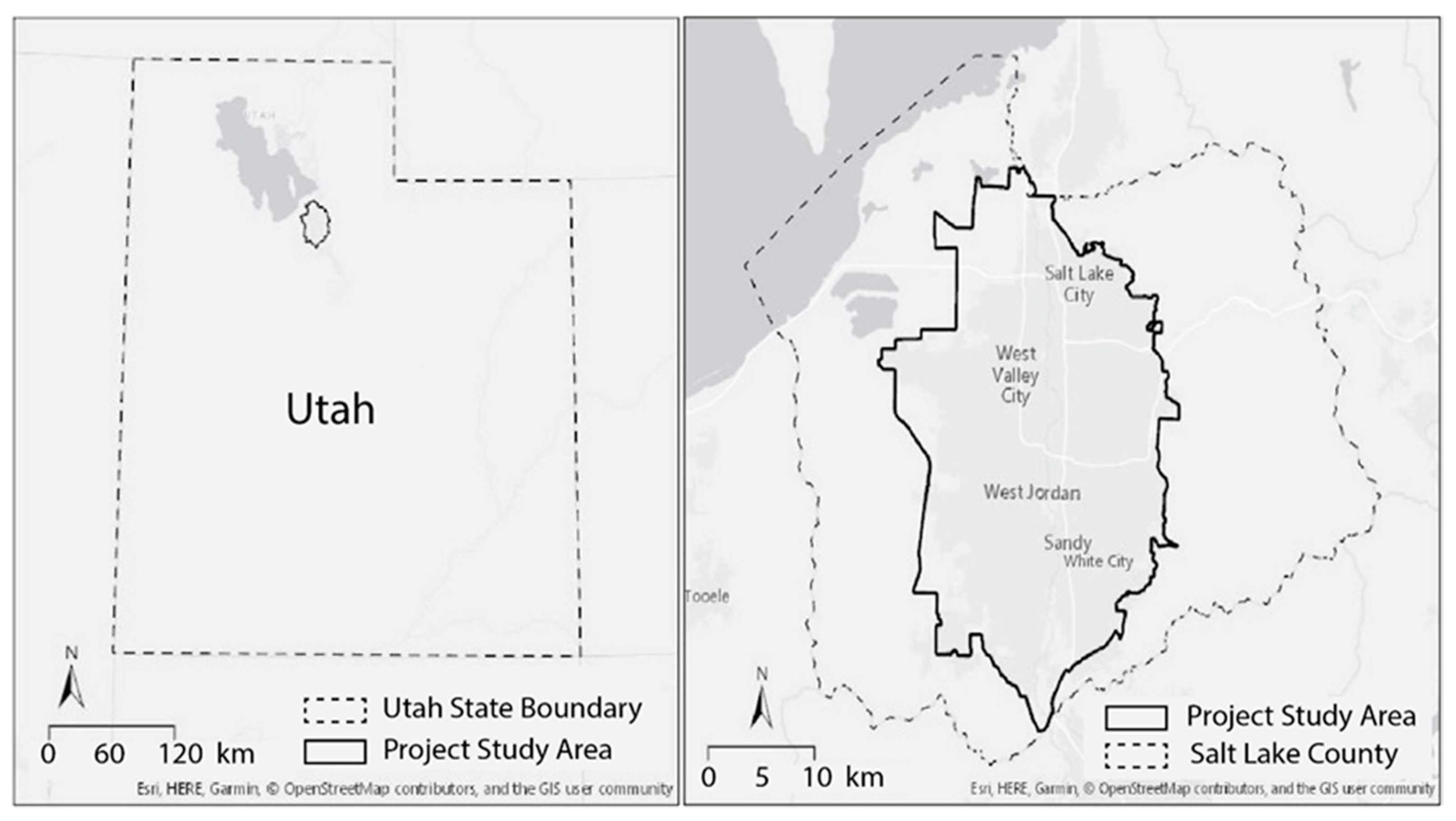
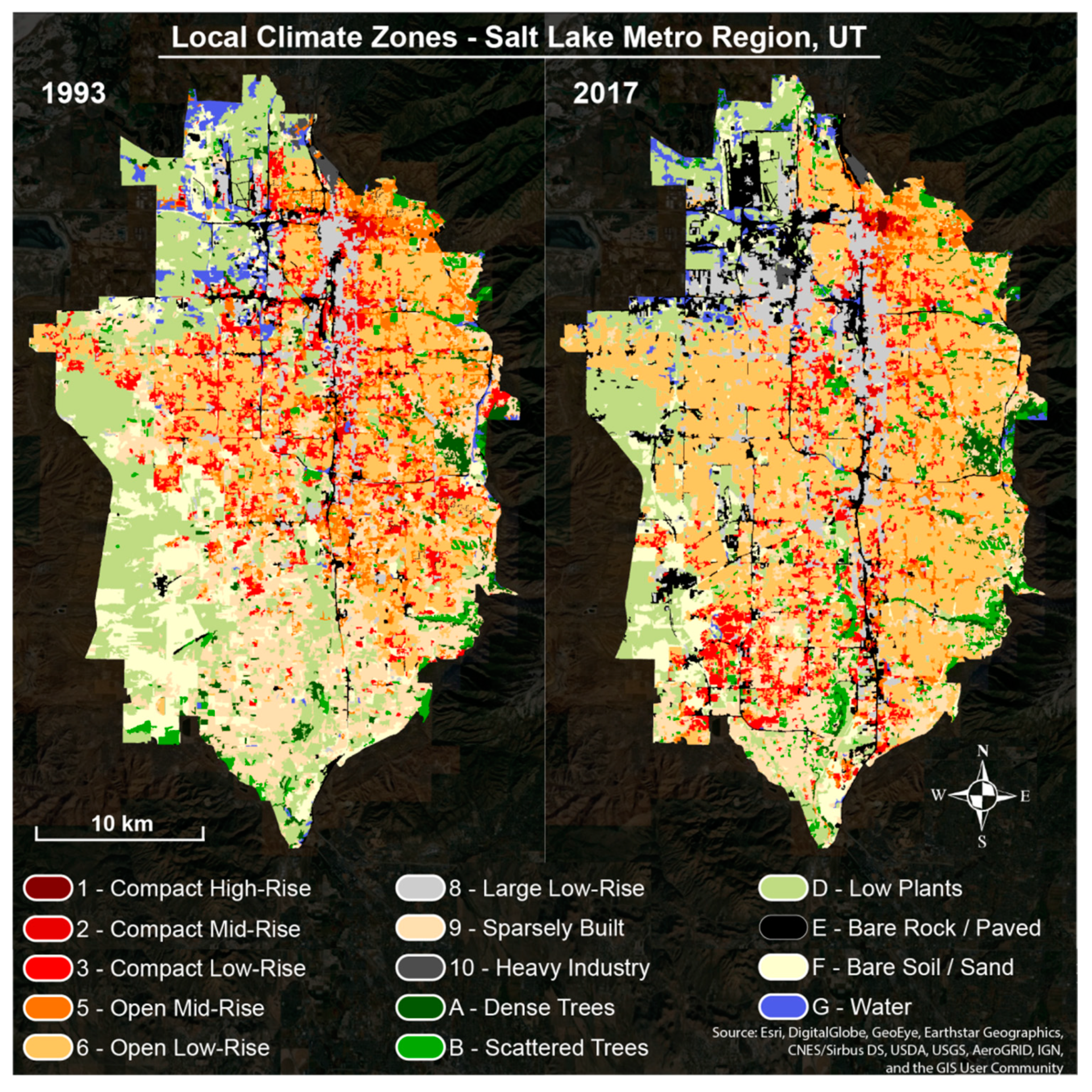
3.1. Study Area

The focal urban area of this study (Figure 1) was the Salt Lake Valley within the State of Utah, USA. It forms the central section of the larger metropolitan region known as the Wasatch Front, within which approximately 80% of the Utah State’s population resides. Surrounded by the Wasatch Mountain Range to the East, the Oquirrh Mountains to the West, and the Great Salt Lake to the Northwest, the study area constitutes a mountain valley. While most of the state of Utah is comprised of desert and semiarid steppe lands, the Wasatch Front forms a humid continental-hot summer zone at 1288 m elevation, with cold, snowy winters averaging below 0 °C, and hot, dry summers averaging around 25 °C. Furthermore, while short-term weather patterns are not necessarily indicative of larger climatic trends, the five warmest years on record for Salt Lake City have all occurred recently, between 2012 and 2017.

Pronounced urban development makes the Salt Lake Valley a particularly relevant place for LCZ analysis, as it is one of the fast-growing metro regions, by population, in the United States. Within the study period of 1993 to 2017, the population increased by approximately 323,000 (40%) [70], while the 2017 average annual percent change in population growth for Salt Lake County in 2017 was 1.27, compared to 0.72 for the entire USA [70]. Furthermore, the proportion of population increase due to migration is growing, which can be attributed to Utah’s booming tech economy [71]. In January 2017 the Salt Lake Metro region had the lowest unemployment rate among all metro areas in the United States with greater than 1 million people [72]. As a result, the urban built up area has also expanded rapidly over the study period, primarily into the southwestern part of the region constrained by the Oquirrh Mountains bordering the West of the Valley. This has caused major changes in land uses and urban morphology within the existing urban footprint, thus providing an informative case for investigating changes in the extent and spatial pattern of LCZs. For this analysis, the study area boundary (Figure 1) was selected to capture the built-up area within Salt Lake County Utah based on 2010 US Census block group polygon geometries. To focus on the main urban extent, polygons that primarily overlaid the desired built up area were selected and combined to form the final boundary, whereas some large or irregularly shaped polygons that extended far outside the desired study area were omitted. Subsequently, object-based image classification was used to classify LCZs from the input Landsat satellite imagery separately for 2017 and 1993, followed by a post-classification change analysis, as described in the following sections (Figure 2).

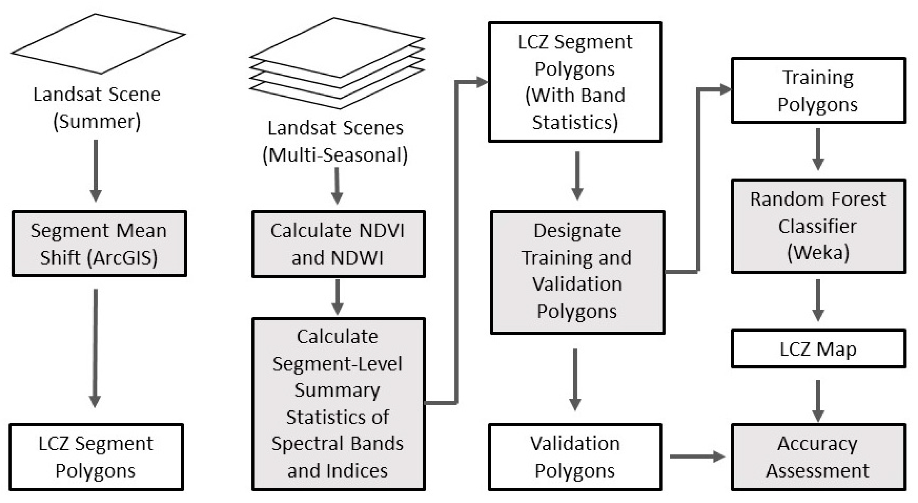
3.2. Object-Based Classification of LCZs from Satellite Imagery

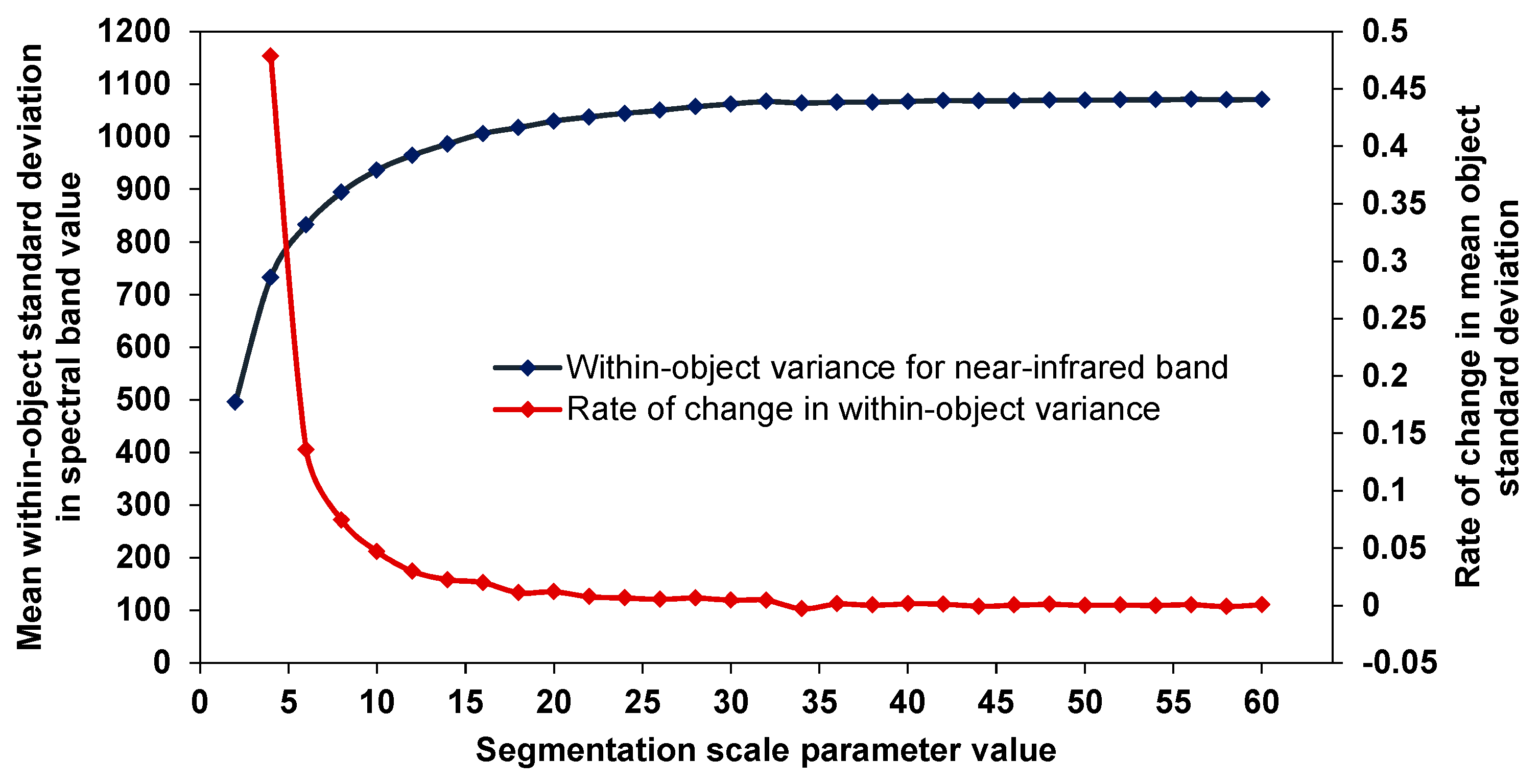
3.2.1. Remote Sensing Data and Image Segmentation

The first step in each year’s LCZ classification was generation of primitive mapping units (i.e., objects) via segmentation of a single-date Landsat image using the Segment Mean Shift tool in ArcGIS version 10.5 (ESRI Inc.) software. Such an algorithm can also be implemented in open-source GIS software, such as QGIS. Segmentation was performed using one satellite image for each time period of interest, representative of the summer-early fall time frame when atmospheric temperatures tend to be higher and annual herbaceous vegetation is typically senescent, highlighting their contrast with woody species (

Table 1. Landsat satellite imagery used in object-based segmentation and classification of LCZs.

	2017 Period			1993 Period
Analysis	Scenes	Date	Bands/Indices	Scenes	Date	Bands/Indices
LCZ (primitive) Segmentation	LC08_L1TP_038032_20170722_20170728_01_T1	22 July 2017	3,4,5	LT05_L1TP_038032_19930922_20160928_01_T1	22 September 1993	2,3,4
LCZ Classification	LC08_L1TP_038032_20170212_20170228_01_T1	12 February 2017	2 3 4 5 6 7 10 11 NDVI NDWI	LT05_L1TP_038032_19930720_20160927_01_T1	20 July 1993	1 2 3 4 5 6 7 NDVI NDWI
	LC08_L1TP_038032_20170401_20170414_01_T1	1 April 2017		LT05_L1TP_038032_19930922_20160928_01_T1	22 September 1993
	LC08_L1TP_038032_20170722_20170728_01_T1	22 July 2017		LT05_L1TP_038032_19931211_20160927_01_T1	11 December 1993
	LC08_L1TP_038032_20171010_20171024_01_T1	10 October 2017		LT05_L1TP_038032_19940402_20160927_01_T1	2 April 1994

). For 1993, the input image was a Landsat 5 Thematic Mapper, Level 1 Precision Terrain Corrected, Tier 1 product, collected on 22 September 1993 (this date was chosen as the closest to the timing of the available digital orthophoto quad high spatial resolution reference imagery of 10 September 1993). Bands 2 (0.52–0.60 µm), 3 (0.63–0.69 µm), and 4 (0.76–0.90 µm) from this image were used in segmentation. For 2017, the input image was a Landsat 8 OLI/TIRS, Level 1 Precision Terrain Corrected, Tier 1 product, collected on 22 July 2017. Landsat bands 3 (0.533–0.590 µm), 4 (0.636–0.673 µm), and 5 (0.851–0.879 µm) from this image were used in segmentation. Electromagnetic regions of these bands correspond to the green, red, and near-infrared spectral wavelengths, expected to help differentiate between green and senescent vegetation, water and built-up/impervious surfaces. Here and later during classification, Landsat images were used at their original spatial resolution of 30 m for visible and infrared bands, and 120 m spatial resolution of thermal bands resampled to 30 m. All satellite images in this study were obtained from the U.S. Geological Survey’s Earth Explorer database (https://earthexplorer.usgs.gov).

The Segment Mean Shift tool in ArcGIS software generates objects via a bottom-up, region-growing algorithm which groups the neighboring pixels together depending on the criteria for spectral similarity, spatial properties of resulting regions and minimum object size determined by a set of user-specified parameters (

Table A1. Main parameters of the segmentation process as the first stage of OBIA workflow.

Parameter	Explanation	Value
		1993	2017
Input Raster	The raster data to segment	LT05_L1TP_038032_19930922_20160928_01_T1	LC08_L1TP_038032_20170722_20170728_01_T1
Band Indexes	Landsat bands used to segment the imagery	Band 2 (0.52–0.60 µm) Band 3 (0.63–0.69 µm) Band 4 (0.76–0.90 µm)	Band 3 (0.533–0.590 µm) Band 4 (0.636–0.673 µm) Band 5 (0.851–0.879 µm)
Spectral Detail	A parameter in Segment Mean Shift tool controlling the importance of spectral differences for the object outcomes. Values range from 1 to 20 with higher values producing greater separation of regions with similar spectral properties.	20	20
Spatial Detail	A parameter controlling the importance of proximity between objects. Values range from 1 to 20, where higher values allow delineating smaller and more clustered features.	2	2
Minimum Segment Size	A scale parameter controlling the size of the smallest allowed objects (in pixels). Objects smaller than this size can be merged with their most similar neighbor.	20	20

, Appendix; [73,74]). The parameter that controls the importance of spectral properties was set to the maximum value of 20 (on the scale from 0 to 20) because it was intended to achieve the greatest discrimination between features with similar spectral characteristics (such as vegetated classes). The parameter for relative importance of spatial detail (Table A1, Appendix) was informed by testing multiple values and visually examining the output against base map imagery, which suggested that the relatively low value of 2 (on the scale from 0 to 20) was optimal for preserving landscape element mixtures relevant to LCZ definitions.

Finally, the parameter controlling segmentation affects the amount of spectral variation allowed within segments and thus minimum segment size (the same amount of local variation in more homogenous landscapes would be captured by larger segments than in heterogeneous areas). Due to potential variability in the size of LCZs, the goal of segmentation was not to delineate their complete extents, but instead to obtain object primitives that could be classified to reproduce such full extents. Thus, segmentation outcomes would ideally sufficiently capture minimum representative groupings of real-world objects and covers for different local climate zone types. To determine the appropriate minimum segment size given these objectives, 30 iterations of the segment mean shift tool were run on the input images, while varying the parameter on each iteration, from 2 to 60 by increments of 2. For each resulting segmented map, the spectral variation within each segment was summarized as the standard deviation of the near infrared band of the input image, and the mean of these within-segment standard deviations was used to summarize within-segment variation for the entire map, and to compare the output maps to one another. Scale parameter value of 20 was chosen for primitive object generation as the inflection point after which the rate of change in within-segment variation starts slowing towards saturation (Figure 3).

3.2.2. Image Classification

Next, the resulting segment polygons were classified into LCZs using the following process. For each time period, four cloud-free Landsat scenes (one for each season) were used (Table 1) in order to capture phenological variation in LCZs that may aid in their classification (Bechtel et al., 2015). For each primitive object in the segmentation results, basic summary statistics (minimum, maximum, mean, median and standard deviation) were calculated for each spectral band for each date. For 2017, training samples of LCZ classes (

Table 2. Local climate zone (LCZ) classes used in classification and change analysis of the study area. Columns labeled with ‘T’ show numbers of training sample objects, and columns labeled ‘V’ show the number of validation samples (2017 only).

LCZ	2017		1993		LCZ	2017		1993
	T	V	T	V		T	V	T	V
2: Compact Mid-Rise	31	31	20	n/a	A: Dense Trees	32	31	60	n/a
3: Compact Low-Rise	32	32	20	n/a	B: Scattered Trees	39	39	20	n/a
5: Open Mid-Rise	38	37	30	n/a	D: Low Plants	40	39	30	n/a
6: Open Low-Rise	42	41	40	n/a	E: Bare Rock or Paved	31	31	40	n/a
8: Large Low-Rise	42	41	40	n/a	F: Bare Soil or Sand	37	37	60	n/a
9: Sparsely Built	33	33	60	n/a	G: Water	31	30	40	n/a

) were then selected following their definitions in [6] from ArcGIS and Google Earth high resolution imagery for 2017 (see examples of class patterns in Figure A1, Appendix). A total of 60 segments were selected to represent each class using a random sampling technique where 100 segments within the study area were selected randomly and each was manually classified by visually interpreting their identity from reference imagery. This process was then repeated until each local climate zone class had accumulated a minimum of 60 samples. However, some classes were not prevalent enough within the study area to achieve the desired 60 samples using this methodology, so specific instances of these classes were sought out, classified manually and isolated prior to automated classification. Specifically, for LCZs 1 (compact high-rise) and 10 (heavy industry), all segments within the study area had been sufficiently identified, and therefore did not need to be included in the supervised image classification. It was discovered that classes 4 (open high-rise) and 7 (lightweight low-rise) could not be identified in the study area, while class C (brush, scrub) could not be reliably distinguished from low plants via visual interpretation alone. Therefore, the resulting candidate LCZs for classification included 2, 3, 5, 6, 8, 9, A, B, D, E, F, and G. For each of them, 50% of the previously identified samples were randomly selected for use in classifier training, and the remaining 50% were reserved for independent accuracy assessment.

For 1993, training sample selection followed a slightly different process since there was no high-resolution reference imagery in Google Earth (Table 2). The best historical (1993) data available for reference were black and white U.S. Geological Survey digital orthophoto quadrangles at 1-m resolution from September 10, 1993. Coverage of the study area by this imagery was also limited; therefore, the number of training samples for each class varied (Table 2). The polygon data representing training sample segments was converted to csv file format for the subsequent LCZ classification.

Next, the open-source Waikato Environment for Knowledge Analysis (Weka) software [75] was used for the supervised classification of each Landsat image set into LCZs based on the identified training samples. The advantage of machine-learning methods for LCZ mapping is that, in contrast to maximum likelihood approaches, they often do not rely on rigid assumptions about class statistical distributions and can handle large numbers of discriminating features that may be useful for complex typologies. In our workflow, the Random Forest classifier recommended by WUDAPT was applied in both years. It was implemented using Weka’s graphical user interface (GUI) with the specification as shown in

Table A2. The following table lists the essential parameters used in setting up the random forest classifier in Weka. Default values were used for all other parameters not listed in the table.

Parameter Name	Value Used	Parameter Description
numIterations	100	The number of trees in the forest.
maxDepth	0 (unlimited)	The maximum depth of each tree.
numFeatures	0 = (log_2(n_features) + 1)	The number of features to consider when looking for the best split
bagSizePercent	100	Size of each bag, as a percentage of the training set size.

, Appendix. For details on how to run Weka the reader is referred to the supporting documentation at https://www.cs.waikato.ac.nz/ml/weka/documentation.html and to [75]. To maintain comparability with other studies using the WUDAPT method, a similar feature set was used, but with the addition of the Normalized Difference Vegetation Index (NDVI; normalized difference between near-infrared and red bands, [76]) and the Normalized Difference Water Index (NDWI; normalized difference between green and near-infrared bands, [77]), following previous studies [50,78]. For the 2017 period, the Landsat 8 feature set included the segment-level means of bands 2-7, 10, 11, NDVI and NDWI, while the 1993 Landsat 5 feature set included the segment-level means of bands 1-7, NDVI and NDWI.

Independent accuracy assessment was subsequently conducted for 2017 using the previously designated validation samples. Accuracy was assessed with the standard metrics (i.e., overall, user’s and producer’s accuracies) based on the contingency matrix comparing reference and mapped identities of the classified LCZs for validation samples [79]. In addition, a bootstrapping procedure was applied using the Python package, Scikit-learn [80] to evaluate the distributions of overall classification accuracy, kappa, overall accuracy of urban-only LCZs and overall accuracy of two aggregated classes, urban (LCZs 1-10) and natural (LCZs A-D, F and G excluding E common to both urban and natural areas), following [30]. No independent accuracy assessment was conducted for 1993 due to the lack of reference data, but the same method and similar input features (Table 1) were used here as for 2017.

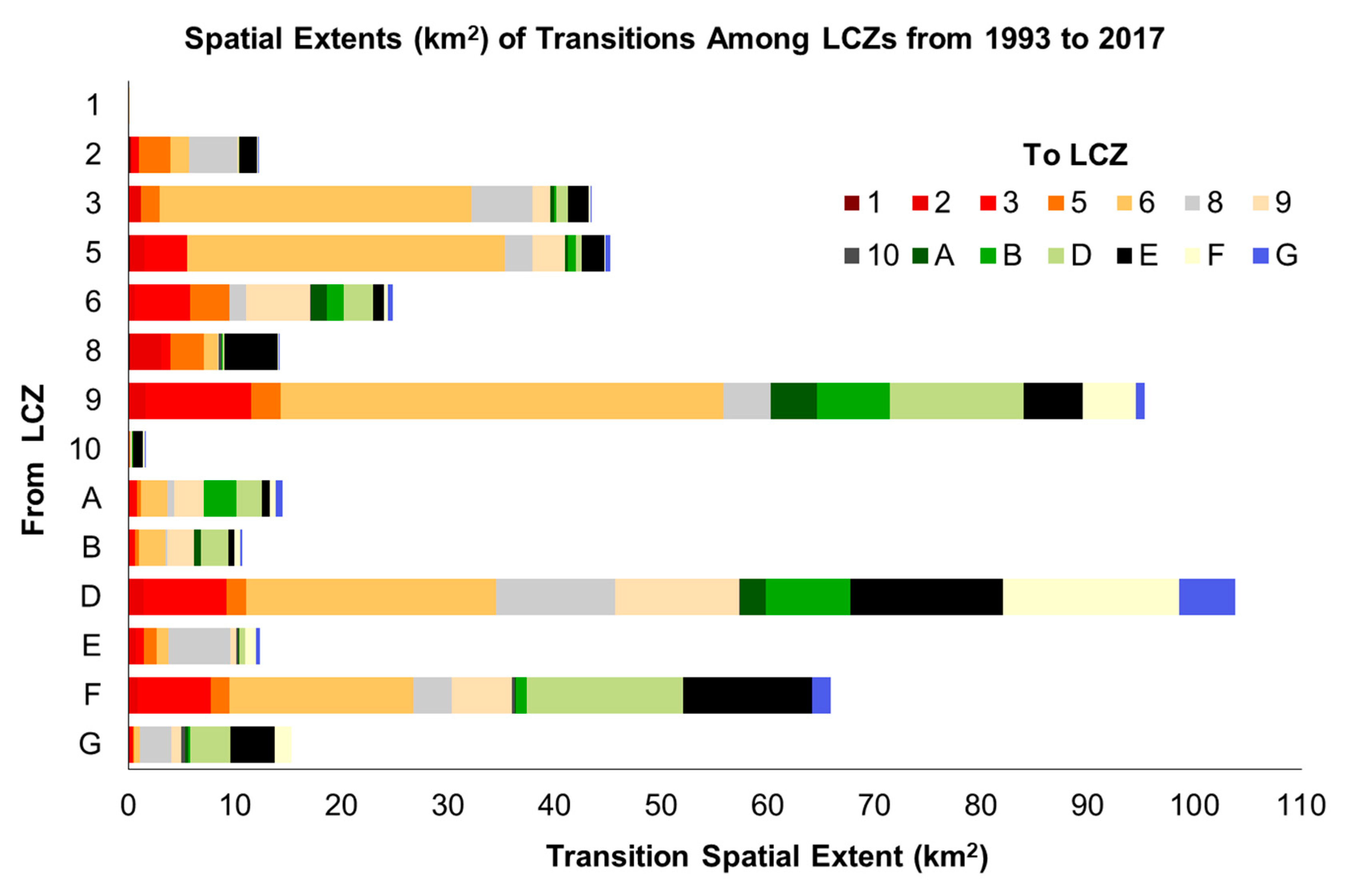
3.3. LCZ Change Analysis

A post-classification change analysis was conducted by computing the geometric intersection of the 1993 and 2017 LCZ maps. Areas where different LCZs intersected were categorized as areas of change, and the specific type of change was labeled according to the previous (From) and current (To) LCZ classes. The sum area of each LCZ was calculated for each analysis year, and the change in LCZ proportional composition of the study area was analyzed. The sum areas of each specific ‘from-to’ change type were also analyzed for the original individual LCZs and for specific LCZ groups sharing similarity in both definitions and directions of change.

Finally, we estimated changes in two landscape metrics characterizing spatial pattern of individual LCZs: mean patch size, representing the average extent of LCZ patches in each respective period, and mean proximity index characterizing the degree of isolation among patches given their size [81]. The latter index can distinguish among scattered, smaller patches (low mean proximity index values) and clusters of larger, more aggregated patches (high mean proximity value).

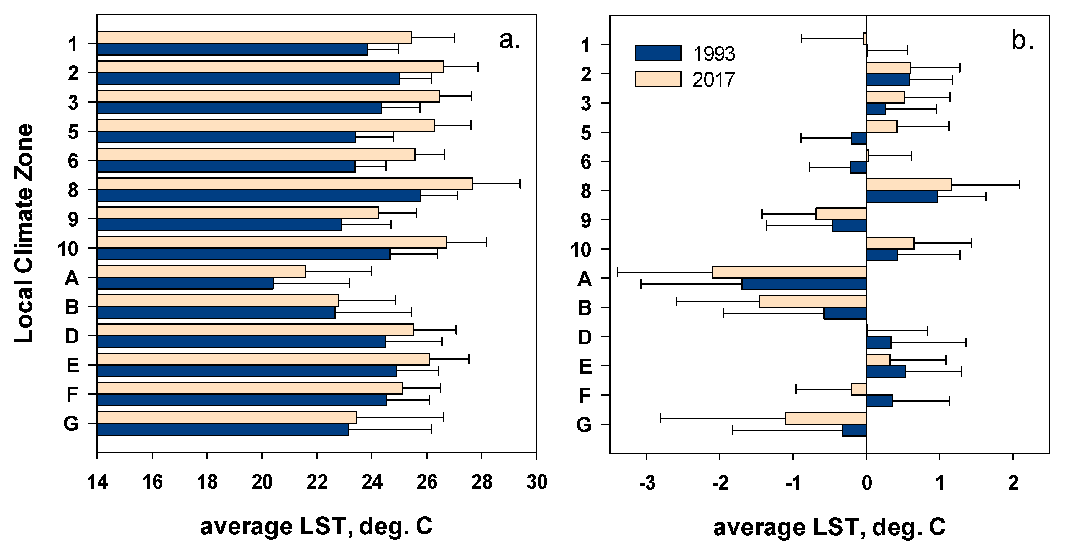
3.4. Changes in the Proxy of Surface Temperature

To investigate the potential microclimatic implications of the observed LCZ changes, we used the land surface temperature (LST) datasets from the Landsat Level-2 Provisional Surface Temperature (ST) Science Products [82] for the same dates as the Landsat images used in classification (Table 1). Between two periods, these selected Landsat dates represented similar seasons and vegetation phenology stages (Table 1). Thus, to compare them, we computed per-pixel annual LST averages and then quantified changes in their mean values for each LCZ between two periods. To assess potential changes in LST distribution within the study area, we also normalized the annual average LSTs within its boundary by subtracting their mean values and dividing by standard deviation. We then evaluated how the skewness and kurtosis of the normalized value distributions changed between two periods.

4. Results

4.1. Supervised Classification of LCZs

The overall accuracy of the 2017 LCZ classification was 64% with kappa coefficient of 0.61 (

Table 3. Contingency matrix for LCZ classification accuracy assessment.

Mapped LCZs	Reference LCZs												User’s Accuracy
	2	3	5	6	8	9	A	B	D	E	F	G
2	12	2	5	0	2	1	0	0	0	2	0	0	0.50
3	2	18	2	4	1	0	0	0	0	2	0	1	0.60
5	8	4	18	0	5	0	0	0	1	3	0	0	0.46
6	0	1	5	37	0	3	2	0	1	0	1	1	0.73
8	3	3	2	0	26	0	0	0	0	5	1	0	0.65
9	0	0	2	0	0	24	2	1	3	0	0	1	0.73
A	0	1	1	0	0	0	22	2	0	0	0	2	0.79
B	0	1	0	0	0	2	5	21	7	0	0	1	0.57
D	0	0	0	0	0	2	0	14	25	0	2	1	0.57
E	5	1	1	0	4	0	0	0	0	18	2	1	0.56
F	1	0	1	0	2	1	0	0	1	1	29	1	0.78
G	0	1	0	0	1	0	0	1	1	0	2	21	0.78
Producer’s Accuracy	0.39	0.56	0.49	0.9	0.63	0.73	0.71	0.54	0.64	0.58	0.78	0.70	Overall accuracy 0.64

), while the cross-validation accuracy initially performed by Weka using the training set was 71% (with kappa equal to 0.68). Overall accuracy distribution determined by bootstrapping largely varied between these two estimates (Figure A2 Appendix), showing a mean value of 0.67. Furthermore, similar to the results in [30], bootstrapping produced relatively lower accuracy values for urban-only LCZs, with the minimum values reaching ~0.55 (Figure A2 Appendix) and a mean of 0.62. In turn, simplifying the scheme to natural versus urban LCZs showed a highly successful distinction of these groups with overall accuracies exceeding 91% (Figure A2 Appendix), also similar to the results in [30].

The individual class accuracies in the independent assessment (Table 3) indicated several notable successes and challenges. Open Low-Rise (LCZ 6), the most prevalent class in 2017 (Figure 4), had the highest producer’s accuracy at 90%. It was followed by Bare Soil (Class F) with 78%, Sparsely Built LCZ 9 (73%) and Dense Vegetation (71%). The highest user’s accuracy was observed for distinct, predominantly non-built-up classes (Table 3): Dense Vegetation (79%), Bare Soil or Sand (78%) and Water (78%).

In contrast, a substantial amount of the classification error was associated with LCZs representing a greater intensity of development, as suggested by the off-diagonal counts in Table 3. For instance, Compact Mid-Rise (LCZ 2) and Open Mid-Rise (LCZ 5) both had the lowest producer and the lowest user accuracies of all classes (Table 3). They also showed a substantial mutual confusion with each other (Table 3). Other notable class pairs with mutual confusion were Paved (LCZ E) and Large Low-Rise (LCZ 8), likely due to their common association with flat impervious surfaces, and between Scattered Trees (LCZ B) and Low Plants (LCZ D), likely due to high prevalence of low-height vegetation in each. User’s accuracy for the Open Low-Rise (LCZ 6) was relatively lower (73%), which together with its higher producer’s accuracy suggested that other classes were likely to be misclassified as this LCZ (Table 3).

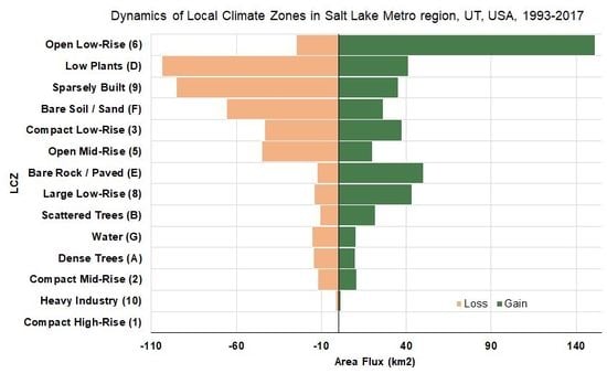
4.2. Change in LCZ Distributions

Spatial distribution and prevalence of LCZs in 1993 and 2017 (Figure 4 and Figure 5) indicated a substantial degree of urbanization during this period (

Table A3. Spatial extents (km²) of transitions and no-change among LCZs from 1993 to 2017.

		TO LCZ (2017)
		1	2	3	5	6	8	9	10	A	B	D	E	F	G
FROM LCZ (1993)	1	0.24	0.01	0.00	0.01	0.00	0.00	0.00	0.00	0.00	0.00	0.00	0.00	0.00	0.00
	2	0.20	2.27	0.70	3.00	1.73	4.55	0.05	0.00	0.02	0.00	0.12	1.65	0.11	0.06
	3	0.00	1.16	4.80	1.67	29.34	5.68	1.67	0.01	0.34	0.18	1.17	1.95	0.14	0.10
	5	0.07	1.42	3.99	6.66	29.76	2.59	3.06	0.02	0.29	0.73	0.56	2.08	0.14	0.45
	6	0.04	0.57	5.12	3.69	117.43	1.61	5.99	0.02	1.48	1.63	2.77	1.01	0.39	0.45
	8	0.11	2.93	0.87	3.11	1.25	21.14	0.16	0.30	0.00	0.05	0.15	4.98	0.15	0.03
	9	0.00	1.58	9.86	2.83	41.49	4.45	35.23	0.02	4.35	6.81	12.50	5.57	5.02	0.78
	10	0.00	0.00	0.00	0.10	0.05	0.06	0.12	1.04	0.01	0.02	0.02	0.94	0.16	0.10
	A	0.00	0.09	0.63	0.36	2.52	0.66	2.74	0.00	6.15	3.06	2.41	0.73	0.55	0.67
	B	0.00	0.10	0.44	0.42	2.49	0.17	2.48	0.00	0.66	6.25	2.61	0.53	0.57	0.12
	D	0.00	1.36	7.82	1.83	23.46	11.14	11.69	0.04	2.37	7.94	61.09	14.35	16.54	5.20
	E	0.01	0.64	0.72	1.22	1.10	5.81	0.55	0.25	0.04	0.01	0.54	11.16	1.02	0.42
	F	0.00	0.80	6.91	1.75	17.27	3.57	5.65	0.23	0.10	0.99	14.68	12.14	14.69	1.78
	G	0.00	0.20	0.18	0.13	0.55	2.91	0.94	0.39	0.28	0.21	3.74	4.12	1.63	2.91

Appendix). Open Low-Rise (LCZ 6) increased from being the second largest (17.4% of the study area) to the most prevalent (35%) in 2017. This class showed the largest gains overall, adding 126.3 km² (88.5% of its 1993 extent), equivalent to 16.8% of the study area (

Table A4. Changes in spatial extents of mapped Local Climate Zones between 1993 and 2017.

LCZ	1993		2017		Area Lost (km2)	Area Gained (km2)	Net Change (km2)	Net Change (As %Class Area)	Net Change (As %Study Area)
	Area (km2)	%Study Area	Area (km2)	%Study Area
1	0.3	0.0	0.7	0.1	0.03	0.44	0.41	155.3	0.1
2	14.5	1.9	13.1	1.7	12.19	10.86	−1.33	−9.2	−0.2
3	48.2	6.4	42.1	5.6	43.40	37.26	−6.15	−12.7	−0.8
5	51.8	6.9	26.7	3.6	45.17	20.12	−25.05	−48.3	−3.3
6	142.6	19.0	268.9	35.8	24.78	151.00	126.22	88.5	16.8
8	35.2	4.7	64.3	8.6	14.10	43.19	29.09	82.6	3.9
9	130.5	17.4	70.3	9.4	95.26	35.10	−60.17	−46.1	−8.0
10	2.6	0.3	2.3	0.3	1.57	1.29	−0.28	−10.8	0.0
A	20.6	2.7	16.1	2.1	14.44	9.94	−4.50	−21.8	−0.6
B	16.8	2.2	27.9	3.7	10.60	21.63	11.04	65.5	1.5
D	164.8	22.0	102.4	13.6	103.74	41.29	−62.45	−37.9	−8.3
E	23.5	3.1	61.2	8.2	12.33	50.06	37.73	160.6	5.0
F	80.6	10.7	41.1	5.5	65.88	26.42	−39.46	−49.0	−5.3
G	18.2	2.4	13.1	1.7	15.28	10.16	−5.11	−28.1	−0.7

Appendix). This was consistent with the population growth observed during the study period, as LCZ 6 typically corresponded with residential suburban development.

Other substantial gains in area were observed in the Paved (LCZ E) and Large Low-Rise (LCZ 8) classes, adding, respectively, 160.6% and 82.35% of their 1993 extents (Figure 5, Table A4 Appendix). By their definition and distribution within the study area, these classes both typically corresponded with commercial and manufacturing uses, the growth of which can also be visually identified on the Local Climate Zone maps. In contrast, the two other most extensive 1993 LCZs, Low Plants (LCZ D) and Sparsely Built (LCZ 9), decreased by 37.9% and 46.1%, respectively, even though both remained among the 3 largest classes in 2017 (Table A4 Appendix). Area losses for these classes together with a 49% decrease in Bare Soil and Sand (LCZ F) indicates that all three likely represented preferred sites for new development. Among most classes that already had been developed in 1993, losses were relatively small, with the exception of Open Mid-Rise (LCZ 5), which lost 48.3% of its area, and Compact Low-Rise (LCZ 3), a large part of which was converted to Open Low-Rise (LCZ 6). Both of the latter results were not intuitive, and in addition to potential LCZ transitions, they could be caused by the classification error and potential expansion of vegetation cover. For instance, growth of woody species or introduction of specific landscaping practices could affect the balance between vegetated and built-up spectral contributions, making the respective locations more similar to LCZ 6.

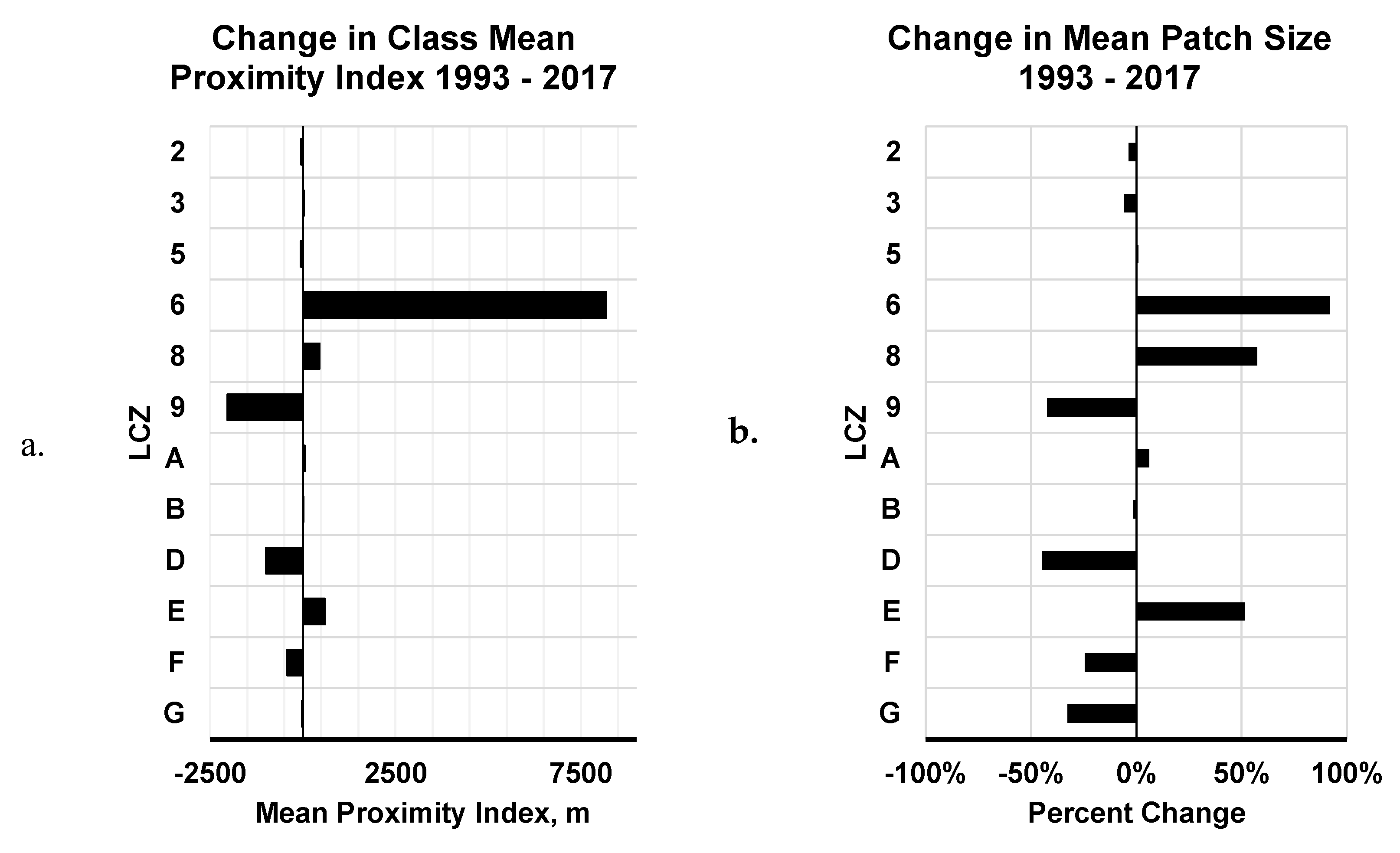
4.3. Changes in Spatial Pattern of LCZ Distribution

The spatial pattern of LCZ distribution also showed several notable changes during the study period. Mean proximity index increased substantially for LCZs 6, 8, and E (Figure 6a), resonating with the large net increases in their respective class areas (Figure 6b, Table A4 Appendix). Among these, LCZ 6 in particular showed an extreme increase, indicating that its expansion was accompanied by greater local aggregation, likely due to extension of existing patches (as opposed to new leapfrog development). While some relatively isolated patches of LCZ 6 remained in the southwestern part of the study area (Figure 4), its mean patch size nearly doubled over the study period (Figure 6b).

In contrast, LCZs 9, D, and F, the classes that showed substantial net decreases in class area, all decreased in mean proximity index as well. On the 1993 map, LCZ 9 formed an aggregated and relatively large grouping of patches in the South and Southwest portions of the study area. This region is where much landscape change took place. Other LCZs, primarily LCZ 6, expanded into this region, forming a more heterogeneous patchwork of LCZs. By looking at the LCZ maps (Figure 4), LCZ 9 clearly shows change to a more fragmented pattern of smaller patches. The mean patch size of LCZ 9 also decreased by approximately 45%.

4.4. Changes in Thermal Characteristics of the Urban Landscape

Finally, the comparison of Landsat land surface temperature variation across the study area between 1993 and 2017 revealed a pronounced overall warming (Figure A3 Appendix), and increases from 0.1 to 2.9 °C on average temperature of individual LCZs (Figure 7a). Pixels with net decreases in temperature represented ~15% of the study area, corresponding to small wetland features, vegetated areas, golf courses and a few urban shadow areas in high-rise neighborhoods. In 1993, the highest mean temperatures were observed for LCZ 8 (25.8 °C) followed by LCZs 2, 10 and E (>24 °C in each). In 2017, LCZs 8 and 10 remained the warmest on average (27.7 and 26.7 °C, respectively), followed by 2, 3, E and 10 (26.1–26.6 °C). The lowest temperatures, in turn, were observed for types A and B in both 1993 (20.4 and 22.7°C, respectively) and in 2017 (21.5 and 22.8°C, respectively). The highest increases in mean LST (>2°C) were observed for open LCZs 5 and 6, compact low-rise (LCZ 3) and industrial (LCZ 10). In turn, the lowest LST changes (within 0.1–1.2°C) corresponded to natural LCZs A–F, indicating that the background thermal conditions did not differ substantially between the two periods.

Mean values of normalized annual average LST indicated that most LCZs remained consistently above or below the study area mean values (Figure 7b). Among natural classes, vegetated (A, B) and water (G) were substantially below the average, while most of the built-up classes were above the average, especially in 2017 (Figure 7b). Two exceptions were Sparsely Built (LCZ 9) with substantial prevalence of non-built cover, and Compact High-Rise (LCZ 1) where lower-than-average LSTs could emerge due to tall building shadows at the time of the satellite overpass. Across the study area, the skewness of normalized LST distributions changed from −0.88 in 1993 to −0.95 in 2017, indicating the increase in the left tail and greater frequency of higher values in the later time period. In turn, the kurtosis of normalized LST distributions has also increased from 7.03 in 1993 to 10.05 in 2017, indicating a greater concentration of values around the mean—i.e., increased homogeneity of the landscape, which may be expected with urbanization.

5. Discussion

5.1. The Informative Value of LCZs for Monitoring Urban Transformation

Major environmental transformations experienced by globally expanding urban regions call for a revision of traditional LULC classes to facilitate the understanding of potential processes underlying these transitions [21,31,53]. The local climate zone framework has been proposed as one of such novel, alternative typologies bridging physical characteristics of cities (and particularly their built environment) with spatial and morphological structural properties applicable to urban architecture, planning and design [9,17,21]. As the appeal of LCZs is recognized by a wider community of researchers and planners and more cities are included in the WUDAPT efforts [20,42], the need to better understand the opportunities offered by different classification approaches (and possibilities to improve them with new methodological advances) is becoming even more pertinent.

A closer look at the transitions among individual LCZs in the study area (Figure 5) highlights the regional tendency towards suburbanization at the expense of lateral low-density development. For example, the largest net increase of the low-density built-up areas (LCZ 6) and relatively low (17%) conversion of their 1993 area to any other class (Table A4 Appendix) suggest that it is not an intermediate stage of development, but rather an ultimate stage. Our results further suggest that much of the new development associated with commercial/industrial land uses (LCZs 8 and E) emerged primarily from direct open space (Figure 4 and Figure 5, Table A3 Appendix) and in some cases sparsely built (LCZ 9) rather than existing low-density development. These patterns are consistent with the broader tendencies in the rapidly urbanizing Wasatch Front of north-central Utah encompassing our study area [83,84]. Developed areas here are projected to expand by 48–80% by 2030, while expected increases in population density range only between 15–25 people/ha, suggesting a prevalence of low-density peripheral urban growth [83]. Similar to urbanizing regions in other parts of USA and Canada [85], such lateral expansion occurs at the expense of agriculturally productive lands and poses multiple threats to natural habitats and ecologically sensitive areas in the region [83,84].

Our results further show that LCZs provide a useful framework to characterize urban transformation [36] and elucidate microclimate-relevant aspects of urban heterogeneity [27,31,50]. Differences in spatial extents and patterns of LCZs between 1993 and 2017 (Figure 4) highlighted the increases in relatively warmer LCZs 8, E and 6 and losses of cooler types A and 9 (Figure 5, Table A4 Appendix). Relative differences in mean brightness temperature among these LCZs (Figure 7) were consistent with earlier studies [29,37,45], although in our case type D (low plants) appeared among the warmer types likely due to dry and warm state of herbaceous natural vegetation in the dry-summer climate of the study area. The overall character of LCZ change showed large increases in LCZs 6, 8, and E, and decreases in LCZs 9, D, and F, which collectively indicate increases in landscape structural and morphological features contributing to potential heat island phenomena. These results were similar to an LCZ change analysis conducted in Bogor City, Jakarta [36], in which an overall trend of increasing area among the built LCZs and decreasing area among the vegetated LCZs was observed along with increases in land surface temperature.

Our results further suggest that potential microclimatic transitions indicated by LCZ changes could be amplified by shifts in their spatial configuration (Figure 6), particularly, consolidation and expansion of LCZs 6, 8 and E, and reduction and fragmentation of LCZs 9, D and F. Hypothetically, not all development transitions should elevate urban heat, particularly when encroaching onto relatively hot open space. For example, Bare Soil (LCZ F) tends to be a relatively warm LCZ in arid and semi-arid cities [45], and thus loss of area and fragmentation of patches of LCZ F may be expected to produce some amount of local cooling if new development adds shading structures, tree and shrub vegetation or irrigation, which may be expected for suburban residential land management. In our case, 35% of the area lost by LCZ F over the study period was replaced by LCZ 6, a class expected to be relatively cooler due to open nature of development and greater vegetation cover (Figure 7), while ~5.6 km² also converted from LCZ F to LCZ 9, another relatively cooler LCZ.

Notably, however, the overall shifts in brightness temperatures in our focal area do not indicate any substantial local cooling (Figure A2 Appendix) with the exception of a few irrigated golf course areas. Furthermore, the increase of average temperatures for all LCZs regardless of the amount of their change (Figure 7, Figure A3 Appendix) suggests that the whole region has experienced an increase in surface temperature between the compared periods. The magnitudes of this increase should be interpreted with caution because they could be influenced by ambient climate warming and the differences between two Landsat instruments and short-term weather fluctuations despite the use of top-of-atmosphere brightness temperature products and their averages over 3-year summer periods. Nevertheless, the observed region-wide warming and shifts in normalized LST distributions were consistent with the expected potential warming due to the expansion of urban area, leading to local temperature increases even in neighborhoods not experiencing changes in urban morphology per se [13,86]. For instance, modeling of summer climate indices based on LCZs in Brno, Czech Republic [86] reported an increase in summer warming indicators for all LCZs under different climate change scenarios, especially the extreme ones.

Importantly, these results imply that microclimates may change without substantial changes in urban morphology defining LCZs, due to synergistic effects of broader-scale urban configuration and increasing ambient and surface temperatures. Changes in urban energy consumption and anthropogenic heat sources could also contribute to thermal shifts without an apparent change in urban morphology [19,87]. These considerations should be taken into account by spatial land use planning and policy to strategically plan for local cooling via landscape design measures to mitigate the broader warming introduced by urban development and promote more sustainable management of water and energy resources [16,19,87,88,89,90]. As many LCZ analyses to date have been performed as single-year, the feedbacks between LCZ-specific microclimates and the broader urban environment represent an important direction for future work.

5.2. Successes and Challenges in Object-Based LCZ Classification

Our results indicate that, overall, object-based image analysis is appealing for classification of Local Climate Zones particularly as high spatial resolution imagery becomes incorporated in such efforts; however, the workflow does not necessarily outperform the successes of previous pixel-based analyses and needs more refinement to become a generalizable framework. Although the overall LCZ classification accuracy of 64% for the full range of considered classes was relatively low, it was comparable with several other previous studies performing supervised classifications of LCZs, such as 56% in [46], 64% in [35] and 67.7% in [42]. Furthermore, most of the classification error was a cumulative outcome of small misclassifications among individual class pairs (Table 3), while the sizable pool of 12 candidate classes and their inherent similarities contributed to greater likelihood of such misclassifications. The observed mutual confusions among LCZs were also common in other studies, particularly the prominent mutual confusion between Compact Mid-Rise (LCZ 2), Large Low-Rise (LCZ 8), and Paved (LCZ E). For instance, [21] noted the misclassification between Large Low-Rise (LCZ 8) and Paved (LCZ E), while [44] reported confusion between the compact built zones and Large Low-Rise (LCZ 8).

Our results further suggest that these confusions may result from both vertical (i.e., building height and rise) and horizontal (i.e., openness and spatial arrangement) similarities among LCZs (Table 3). Mutual confusions among built-up classes with different levels of building height indicate the limitations of passive remote sensors to capture the differences in rise, while misclassifications among compact and open LCZs suggest potential similarities in relative contributions of their land covers despite the expected differences in configuration. Similarly, substantial confusion among ‘sparse’ LCZs 9, B and D (Table 3) places varying sparseness of woody plant cover as an important challenge for both LCZ mapping and inference of microclimatic properties in less developed and sparsely built areas. This evidence implies that complexity of 3D urban structure is an important contributor to LCZ mapping uncertainties regardless of the classification method. Future work should thus more rigorously explore the utility of datasets representing vertical variability in urban surface, such as novel metrics of building density, tree cover and broader local heterogeneity developed from LiDAR [28] and radar [49] active remote sensing products.

Some of the observed classification successes were likely attributed to the advantages of the OBIA framework, particularly, the high producer’s accuracy for a heterogeneous-by-definition Open Low-Rise (LCZ 6) (Table 3). Using image objects as multi-pixel mapping units may allow capturing complex spatial patterns composed of both constructed elements and various types of open and vegetated spaces between them under the same semantic identity. As open low-rise development appears to be one of the key transformations in the study area’s urban sprawl, these results suggests that the object-based framework may help address the definitional complexity of LCZs as an inherent challenge in their mapping. Our results also suggest that mapping LCZs with potentially larger amounts of vegetation (e.g., A, B, D, 9) can benefit from the OBIA approach as well by helping to separate them from more developed LCZs that may include vegetated pixels as part of, e.g., backyard and street spaces. However, primitive objects generated from moderate-resolution data might not be sufficiently sensitive to nuanced variation in low-density woody cover or presence of sparsely built elements.

Differentiating among such LCZs with confidence may ultimately require higher-resolution imagery [46,48,67], where, again, objects may offer greater flexibility for summarizing local heterogeneity and complex LCZ boundaries compared to square block mapping units [67]. For current and future analyses, such opportunities are emerging with the accumulation of open-access Sentinel-2 imagery and Harmonized Landsat-Sentinel-2 product [91]. Moderate-resolution imagery remains appealing for broad-scale and historical LCZ mapping due to the availability of thermal products and unparallelled archive length. However, emerging urban studies are increasingly uncovering the microclimatic impacts of fine-scale LULC patterns and urban structure [15,16,63,64], which necessarily rely on higher detail of landscape characterization. As such, mechanistic understanding of LCZs and their microclimatic properties would necessarily invoke the applications of high spatial resolution data [51], even if thermal information is not available at the same spatial scales. As the benefits of greater spatial detail come at the cost of greater local spectral noise and confounding heterogeneity, the advantages of OBIA [59,69] and its earlier applications in urban mapping [53,56] may be increasingly useful to LCZ analyses in the future.

The limitations encountered in our OBIA implementation for LCZ mapping call for more research in three important directions. First, OBIA performance, as well as its added cost and logistical demand, should be compared against the established pixel-based workflows, particularly WUDAPT [20,21,30]. The relatively straightforward implementation and universality of the latter are important advantages when urban structure can be well represented by 100–150 m pixel units, as suggested by high classification accuracy in some of the previous studies [21,43,44]. In contrast, OBIA’s possibility to use more flexible and variable mapping units in complex landscapes comes at a cost of extra steps required to parameterize the segmentation and limited generalizability, which may not be equally necessary among different cities. Thus, to provide a more informed guidance about method selection, future research should perform comparative assessments of the alternative workflows in landscapes with different levels of structural and morphological complexity, using high-quality reference data.

Second, the role of segmentation and strategies to optimize the choice of its parameters need to be identified more explicitly, because the degree of spectral heterogeneity in LCZs is expected to vary due to their definitions [58,92]. Although the Segment Mean Shift tool is able to generate variable sizes and properties of primitive objects, the contrasts between more homogeneous LCZs and classes with inherent configurational complexity present the risks for both under-segmentation (i.e., covering more than one visually discernable LCZ) and over-generalization (delineating single homogeneous cover signatures, such as building rooftops, rather than capturing local scale structures). Furthermore, the flexibility of variable-size objects comes at a cost of difficulties to anticipate specific properties of mapping units, which may need to be chosen according to city-specific landscape properties. Thus, a more careful discrimination should be taken in future analyses to choose training objects that are relatively large and “homogeneous” with respect to LCZ definition. Incorporating spatial units that are likely to influence the pattern of development associated with hypothesized LCZ structure—such as land parcels, zoning units or census units sharing similar population and housing densities—may also facilitate this task.

Third, there remains an important uncertainty about which spectral, textural and other features may be most effective at differentiating LCZs given the complexity of their typology (Table 2). Phenological characteristics of vegetation may further contribute to such uncertainties; for example, in dry-summer climates such as in our study area, herbaceous vegetation may be spectrally similar to trees in green stage and to bare soil in senescent stage. More detailed future investigations would thus be useful both at the segmentation stage (since the Segment Mean Shift tool in ArcGIS takes as input 3 user-specified image bands at a time) and at the stage of classification to identify the most useful discriminating features and optimal date(s) [47].

5.3. Other Key Lessons and Future Research Directions

Opportunities and challenges revealed by our analysis suggest several other important future research directions to make LCZ applications more robust and transferable across global regions. There is an obvious need to refine and standardize the validation of LCZ mapping outcomes, because different accuracy assessment strategies in previous studies make it difficult to draw generalized lessons about method performance. Spatial dimensions of testing units may also affect accuracy assessment; for instance, a study with classification accuracy of 64% similar to ours [35] commented that even independent validation pixels may be problematic as LCZs are supposed to be at least 1 km² in size. To avoid a potential bias due to proximity of training and test samples, in [44], independent validation polygons were purposefully chosen from training areas instead of randomly selected pixels; the resulting overall accuracies ranged from 79.6 to 90.2% in different cities. Lessons from a global LCZ transferability assessment [50] highlight the importance of both training and test sample selections and suggest the need to consider sample sources broader than an individual focal city. A unique challenge in validating object-based LCZ classification thus becomes a decision as to what types of reference objects might perform as the most representative, and what criteria might be especially important in guiding the initial segmentation process to capture their LCZ relevance.

The latter challenge, in turn, highlights another interesting and important research need: developing a stronger understanding of the ‘characteristic’ spatial scales of different LCZs to better inform the minimum mapping unit selection (or segmentation scale in OBIA workflows). Both the original definitions of LCZs and the insights from our results make it obvious that a single segmentation scale or moving window size might not fully accommodate their differences, which has been long recognized in complex landscapes [55,92]. However, in the context of LCZ mapping, it further translates into the need to understand scales that effectively represent thermal outcomes of specific patterns. This understanding is currently limited both by challenges to discriminate among LCZs despite the inclusion of the thermal remote sensing datasets [93] and by the dynamic behavior of urban temperatures that may shift even when morphological aspects of LCZs remain stable. Future studies should therefore more explicitly investigate the fundamental relationships between local spatial patterns and their thermal outcomes across ranges of urban scales beyond individual pixels or multi-pixel square neighborhoods.

Together, these issues also raise important questions about the interpretation and uncertainty of the LCZ boundaries. Urban microclimates are often continuous, scale-dependent [17,20,22,39] and difficult to discretize due to various processes contributing to atmospheric circulation and energy transfer [6]. In contrast, the morphology of LCZs treats urban landscapes as mosaics of discrete semantic entities, e.g., buildings, trees, roads or their groupings, with detectable limits [6]. However, with moderate to coarse spatial resolution units, such as 30 m Landsat pixels or larger sizes recommended by WUDAPT [21,30,42], the boundaries between urban entities and LCZs themselves are likely to be diluted. As such, it can be difficult to interpret the mapped LCZ boundaries based on the local gradients of temperature or other microclimatic parameters. This uncertainty is further augmented by both the shorter-term variation of urban temperatures (e.g., diurnal, seasonal or interannual) and longer-term shifts (e.g., due to continuing urban warming). As a result, spatially explicit validation of LCZs and their boundaries from the urban microclimate perspective remains an important and interesting challenge for the future research.

Finally, an important research need is testing the potential of complementary remote sensing datasets to elucidate structural, configurational and microclimatic differences among LCZs. The ‘ideal’ datasets for characterizing urban 3D complexity, such as LiDAR point clouds or waveform datasets, are not yet available globally as systematically acquired and publicly available products. However, advances in moderate-resolution satellite radar systems, including publicly available Sentinel-1 instruments, may provide useful information about volume and complexity of urban structures to complement the passive optical remote sensing datasets even if thermal bands are not available [43]. Very few studies to date, however, have attempted such multi-source analyses in the context of LCZs, and the utility of radar inputs was not uniformly obvious among their results [43,93]. The earlier mentioned harmonization of Landsat and Sentinel-2 products [91] and emerging higher-resolution open-access land surface temperature datasets [94] would further support such analyses at global scales and repeated time frames.

6. Conclusions

This study classified Local Climate Zones [6] in the Salt Lake Metro Region (USA) and assessed their change between 1993 and 2017 using object-based image analysis with 30-m resolution Landsat data. Our results show that urbanization of the study area during this period was accompanied by several notable LCZ transformations, particularly the expansion of open low-rise development common in residential neighborhoods and large low-rise and paved LCZs common in commercial/industrial areas. Both of these types grew primarily at the expense of non-developed or sparsely built areas and suggested that suburbanization and lateral sprawl, rather than intensification of existing development, were the key players in the observed transformations. While hypothetically the observed transitions could be expected to produce both local warming and local cooling (e.g., due to conversion of bare soil to low-density developed areas with greater green vegetation cover), the mean values for Landsat-based surface temperature increased for all LCZs by 0.1-2.9°C, showing the warming tendency across the vast majority of the region. While our results cannot reliably disentangle urbanization from ambient climate warming, new anthropogenic energy sources and potential confounding effects of satellite data availability, they highlight an important need to investigate thermal dynamics of LCZs which might occur in growing cities without pronounced changes in the morphology of their neighborhoods.

From a practical perspective, our findings indicate that OBIA applied to moderate-resolution satellite imagery shows potential to facilitate LCZ classification and change analysis by capturing local heterogeneity of urban landscapes within objects as mapping units. However, as most of the classification error resulted from the confusions among developed LCZs with varying horizontal density of landscape elements and vertical height of vegetation and built-structures, several important directions should be pursued in future research. These directions include: (1) identifying characteristic spatial scales of different LCZ patterns to more effectively guide segmentation of images into objects as mapping units; (2) testing additional feature sets as discriminating attributes in LCZ classification, particularly, measures of local variance and texture [44,47,66]; and (3) testing the utility of complementary datasets, particularly active remote sensing data, to support LCZ classification by providing additional information on 3D structure and heterogeneity of urban landscapes [43,93].

In sum, our findings concur with previous studies that Local Climate Zones show potential as a valuable framework for landscape change analysis as they can provide a more detailed, climate-relevant perspective of urban change when compared with traditional land use and land cover classification schemes. Our results corroborate the potential of the open-access Landsat imagery to support the analysis of urban microclimatic transformation consistently with the goals of the WUDAPT project and similar initiatives and encourage LCZ classifications for past time periods and more detailed longer-term change assessments.

References

1. Weber, S.; Sadoff, N.; Zell, E.; De Sherbinin, A. Policy-relevant indicators for mapping the vulnerability of urban populations to extreme heat events: A case study of Philadelphia. Appl. Geogr. 2015, 63, 231–243. [Google Scholar] [CrossRef]
2. Jesdale, B.M.; Morello-Frosch, R.; Cushing, L. The racial/ethnic distribution of heat risk-related land cover in relation to residential segregation. Environ. Health Perspect. 2013, 121, 811–817. [Google Scholar] [CrossRef] [PubMed]
3. Reid, C.E.; O’Neill, M.S.; Gronlund, C.J.; Brines, S.J.; Brown, D.G.; Diez-Roux, A.V.; Schwartz, J. Mapping community determinants of heat vulnerability. Environ. Health Perspect. 2009, 117, 1730–1736. [Google Scholar] [CrossRef] [PubMed]
4. Declet-Barreto, J.; Knowlton, K.; Jenerette, G.D.; Buyantuev, A. Effects of urban vegetation on mitigating exposure of vulnerable populations to excessive heat in Cleveland, Ohio. Weather Clim. Soc. 2016, 8, 507–524. [Google Scholar] [CrossRef]
5. Akbari, H. Energy Saving Potentials and Air Quality Benefits of Urban Heat Island Mitigation; Lawrence Berkeley National Laboratory: Berkeley, CA, USA, 2005. Available online: https://escholarship.org/uc/item/4qs5f42s (accessed on 1 April 2019).
6. Stewart, I.D.; Oke, T.R. Local climate zones for urban temperature studies. Bull. Am. Meteorol. Soc. 2012, 93, 1879–1900. [Google Scholar] [CrossRef]
7. Weng, Q. Remote sensing of impervious surfaces in the urban areas: Requirements, methods, and trends. Remote Sens. Environ. 2012, 117, 34–49. [Google Scholar] [CrossRef]
8. Clinton, N.; Gong, P. MODIS detected surface urban heat islands and sinks: Global locations and controls. Remote Sens. Environ. 2013, 134, 294–304. [Google Scholar] [CrossRef]
9. Demuzere, M.; Bechtel, B.; Middel, A.; Mills, G. Mapping Europe into local climate zones. PLoS ONE 2019, 14, e0214474. [Google Scholar] [CrossRef]
10. US EPA, O. Climate Change Indicators in the United States. Available online: https://www.epa.gov/climate-indicators (accessed on 25 April 2019).
11. Luber, G.; McGeehin, M. Climate change and extreme heat events. Am. J. Prev. Med. 2008, 35, 429–435. [Google Scholar] [CrossRef]
12. United Nations Department of Economic and Social Affairs, Population Division. World Urbanization Prospects: The 2014 Revision, Methodology Working Paper No. ESA/P/WP.238, 2014. Available online: https://population.un.org/wup/Publications/Files/WUP2014-Report.pdf (accessed on 20 March 2018).
13. Debbage, N.; Shepherd, J.M. The urban heat island effect and city contiguity. Comput. Environ. Urban Syst. 2015, 54, 181–194. [Google Scholar] [CrossRef]
14. Zhao, L.; Lee, X.; Smith, R.B.; Oleson, K. Strong contributions of local background climate to urban heat islands. Nature 2014, 511, 216. [Google Scholar] [CrossRef] [PubMed]
15. Sun, R.; Lü, Y.; Yang, X.; Chen, L. Understanding the variability of urban heat islands from local background climate and urbanization. J. Clean. Prod. 2019, 208, 743–752. [Google Scholar] [CrossRef]
16. Chen, A.; Yao, X.A.; Sun, R.; Chen, L. Effect of urban green patterns on surface urban cool islands and its seasonal variations. Urban For. Urban Green. 2014, 13, 646–654. [Google Scholar] [CrossRef]
17. Middel, A.; Häb, K.; Brazel, A.J.; Martin, C.A.; Guhathakurta, S. Impact of urban form and design on mid-afternoon microclimate in Phoenix Local Climate Zones. Landsc. Urban Plan. 2014, 122, 16–28. [Google Scholar] [CrossRef]
18. Harlan, S.L.; Brazel, A.J.; Prashad, L.; Stefanov, W.L.; Larsen, L. Neighborhood microclimates and vulnerability to heat stress. Soc. Sci. Med. 2006, 63, 2847–2863. [Google Scholar] [CrossRef] [PubMed]
19. Sikder, S.K.; Nagarajan, M.; Kar, S.; Koetter, T. A geospatial approach of downscaling urban energy consumption density in mega-city Dhaka, Bangladesh. Urban Clim. 2018, 26, 10–30. [Google Scholar] [CrossRef]
20. Brousse, O.; Martilli, A.; Foley, M.; Mills, G.; Bechtel, B. WUDAPT, an efficient land use producing data tool for mesoscale models? Integration of urban LCZ in WRF over Madrid. Urban Clim. 2016, 17, 116–134. [Google Scholar] [CrossRef]
21. Bechtel, B.; Alexander, P.J.; Boehner, J.; Ching, J.; Conrad, O.; Feddema, J.; Mills, G.; See, L.; Stewart, I. Mapping Local Climate Zones for a Worldwide Database of the Form and Function of Cities. ISPRS Int. J. Geo-Inf. 2015, 4, 199–219. [Google Scholar] [CrossRef] [Green Version]
22. Stewart, I.D. A systematic review and scientific critique of methodology in modern urban heat island literature. Int. J. Climathol. 2011, 31, 200–217. [Google Scholar] [CrossRef]
23. Krayenhoff, E.S.; Voogt, J.A. Impacts of urban albedo increase on local air temperature at daily–annual time scales: Model results and synthesis of previous work. J. Appl. Meteorol. Climathol. 2010, 49, 1634–1648. [Google Scholar] [CrossRef]
24. Stewart, I.; Oke, T. Thermal Differentiation of Local Climate Zones Using Temperature Observations from Urban and Rural Field Sites. 9th Symposium on Urban Environment, Keystone, Colorado, 2010. Available online: https://www.researchgate.net/publication/228420685 (accessed on 1 April 2019).
25. Stewart, I.D.; Oke, T.R.; Krayenhoff, E.S. Evaluation of the ‘local climate zone’ scheme using temperature observations and model simulations: Evaluation of the ‘local climate zone’ scheme. Int. J. Climathol. 2014, 34, 1062–1080. [Google Scholar] [CrossRef]
26. Perera, N.G.R.; Emmanuel, R. A “Local Climate Zone” based approach to urban planning in Colombo, Sri Lanka. Urban Clim. 2018, 23, 188–203. [Google Scholar] [CrossRef]
27. Verdonck, M.L.; Demuzere, M.; Hooyberghs, H.; Beck, C.; Cyrys, J.; Schneider, A.; Dewulf, R.; Van Coillie, F. The potential of local climate zones maps as a heat stress assessment tool, supported by simulated air temperature data. Landsc. Urban Plan. 2018, 178, 183–197. [Google Scholar] [CrossRef]
28. Zhao, C.; Jensen, J.; Weng, Q.; Currit, N.; Weaver, R. Application of airborne remote sensing data on mapping local climate zones: Cases of three metropolitan areas of Texas, U.S. Comput. Environ. Urban Syst. 2019, 74, 175–193. [Google Scholar] [CrossRef]
29. Leconte, F.; Bouyer, J.; Claverie, R.; Pétrissans, M. Using Local Climate Zone scheme for UHI assessment: Evaluation of the method using mobile measurements. Build. Environ. 2015, 83, 39–49. [Google Scholar] [CrossRef]
30. Bechtel, B.; Alexander, P.J.; Beck, C.; Böhner, J.; Brousse, O.; Ching, J.; Demuzere, M.; Fonte, C.; Gál, T.; Hidalgo, J.; et al. Generating WUDAPT Level 0 data—Current status of production and evaluation. Urban Clim. 2019, 27, 24–45. [Google Scholar] [CrossRef]
31. Ching, J.; Mills, G.; Bechtel, B.; See, L.; Feddema, J.; Wang, X.; Ren, C.; Brousse, O.; Martilli, A.; Neophytou, M.; et al. WUDAPT: An Urban weather, climate, and environmental modeling infrastructure for the anthropocene. Bull. Am. Meteorol. Soc. 2018, 99, 1907–1924. [Google Scholar] [CrossRef]
32. Bechtel, B.; Conrad, O.; Tamminga, M.; Verdonck, M.L.; Coillie, F.V.; Tuia, D.; Demuzere, M.; See, L.M.; Lopes, P.F.; Fonte, C.C.; et al. Beyond the urban mask. In 2017 Jt. Urban Remote Sens. Event (JURSE); IEEE: Piscataway, NJ, USA, 2017; pp. 1–4. [Google Scholar] [Green Version]
33. Bechtel, B.; Demuzere, M.; Mills, G.; Zhan, W.; Sismanidis, P.; Small, C.; Voogt, J. SUHI analysis using Local Climate Zones—A comparison of 50 cities. Urban Clim. 2019, 28, 100451. [Google Scholar] [CrossRef]
34. Thomas, G.; Sherin, A.P.; Ansar, S.; Zachariah, E.J. Analysis of urban heat island in Kochi, India, using a modified Local Climate Zone classification. Procedia Environ. Sci. 2014, 21, 3–13. [Google Scholar] [CrossRef]
35. Danylo, O.; See, L.; Bechtel, B.; Schepaschenko, D.; Fritz, S. Contributing to WUDAPT: A Local Climate Zone classification of two cities in Ukraine. IEEE J. Sel. Top. Appl. Earth Obs. Remote Sens. 2016, 9, 1841–1853. [Google Scholar] [CrossRef]
36. Nurwanda, A.; Honjo, T. Analysis of land use change and expansion of surface urban heat island in Bogor City by remote sensing. ISPRS Int. J. Geo-Inf. 2018, 7, 165. [Google Scholar] [CrossRef]
37. Geletič, J.; Lehnert, M.; Dobrovolný, P. Land surface temperature differences within Local Climate Zones, based on two Central European cities. Remote Sens. 2016, 8, 788. [Google Scholar] [CrossRef]
38. Wang, C.; Myint, S.; Wang, Z.; Song, J. Spatio-temporal modeling of the urban heat island in the Phoenix Metropolitan area: Land use change implications. Remote Sens. 2016, 8, 185. [Google Scholar] [CrossRef]
39. Hart, M.A.; Sailor, D.J. Quantifying the influence of land-use and surface characteristics on spatial variability in the urban heat island. Theor. Appl. Climatol. 2009, 95, 397–406. [Google Scholar] [CrossRef]
40. Gál, T.; Bechtel, B.; Unger, J. Comparison of two different Local Climate Zone mapping methods. In Proceedings of the ICUC9–9th International Conference on Urban Climate jointly with 12th Symposium on the Urban Environment, Toulouse, France, 20–24 July 2015; Available online: http://www.meteo.fr/icuc9/LongAbstracts/gd2-6-1551002_a.pdf (accessed on 1 March 2018).
41. Lelovics, E.; Unger, J.; Gál, T.; Gál, C. Design of an urban monitoring network based on Local Climate Zone mapping and temperature pattern modelling. Clim. Res. 2014, 60, 51–62. [Google Scholar] [CrossRef]
42. Ren, C.; Wang, R.; Cai, M.; Xu, Y.; Zheng, Y.; Ng, E. The Accuracy of LCZ maps generated by the World Urban Database and Access Portal Tools (WUDAPT) method: A case study of Hong Kong. In Proceedings of the Fourth International Conference on Countermeasures to Urban Heat Islands, Singapore, 30 May–1 June 2016; Available online: https://www.researchgate.net/publication/303753786 (accessed on 1 March 2018).
43. Bechtel, B.; See, L.; Mills, G.; Foley, M. Classification of Local Climate Zones using SAR and multispectral data in an arid environment. IEEE J. Sel. Top. Appl. Earth Obs. Remote Sens. 2016, 9, 3097–3105. [Google Scholar] [CrossRef]
44. Verdonck, M.L.; Okujeni, A.; Van der Linden, S.; Demuzere, M.; De Wulf, R.; Van Coillie, F. Influence of neighbourhood information on ‘Local Climate Zone’ mapping in heterogeneous cities. Int. J. Appl. Earth Obs. Geoinf. 2017, 62, 102–113. [Google Scholar] [CrossRef]
45. Wang, C.; Middel, A.; Myint, S.W.; Kaplan, S.; Brazel, A.J.; Lukasczyk, J. Assessing local climate zones in arid cities: The case of Phoenix, Arizona and Las Vegas, Nevada. ISPRS J. Photogramm. Remote Sens. 2018, 141, 59–71. [Google Scholar] [CrossRef]
46. Kaloustian, N.; Bechtel, B. Local climatic zoning and urban heat island in Beirut. Procedia Eng. 2016, 169, 216–223. [Google Scholar] [CrossRef]
47. Qiu, C.; Schmitt, M.; Mou, L.; Ghamisi, P.; Zhu, X. Feature importance analysis for Local Climate Zone classification using a residual convolutional neural network with multi-source datasets. Remote Sens. 2018, 10, 1572. [Google Scholar] [CrossRef]
48. Oxoli, D.; Ronchetti, G.; Minghini, M.; Molinari, M.; Lotfian, M.; Sona, G.; Brovelli, M. Measuring urban land cover influence on air temperature THROUGH multiple geo-data—The case of Milan, Italy. ISPRS Int. J. Geo-Inf. 2018, 7, 421. [Google Scholar] [CrossRef]
49. Hu, J.; Ghamisi, P.; Zhu, X. Feature extraction and selection of sentinel-1 dual-pol data for global-scale Local Climate Zone classification. ISPRS Int. J. Geo-Inf. 2018, 7, 379. [Google Scholar] [CrossRef]
50. Demuzere, M.; Bechtel, B.; Mills, G. Global transferability of local climate zone models. Urban Clim. 2019, 27, 46–63. [Google Scholar] [CrossRef]
51. Wicki, A.; Parlow, E. Attribution of local climate zones using a multitemporal land use/land cover classification scheme. J. Appl. Remote Sens. 2017, 11, 026001. [Google Scholar] [CrossRef]
52. Wang, Y.; Zhan, Q.; Ouyang, W. Impact of urban climate landscape patterns on land surface temperature in Wuhan, China. Sustainability 2017, 9, 1700. [Google Scholar] [CrossRef]
53. Voltersen, M.; Berger, C.; Hese, S.; Schmullius, C. Object-based land cover mapping and comprehensive feature calculation for an automated derivation of urban structure types at block level. Remote Sens. Environ. 2014, 154, 192–201. [Google Scholar] [CrossRef]
54. Clinton, N.; Holt, A.; Scarborough, J.; Yan, L.; Gong, P. Accuracy assessment measures for object-based image segmentation goodness. Photogramm. Eng. Remote Sens. 2010, 76, 289–299. [Google Scholar] [CrossRef]
55. Holt, A.C.; Seto, E.Y.W.; Rivard, T.; Gong, P. Object-based detection and classification of vehicles from high-resolution aerial photography. Photogramm. Eng. Remote Sens. 2009, 75, 871–880. [Google Scholar] [CrossRef]
56. Williams, D.A.R.; Matasci, G.; Coops, N.C.; Gergel, S.E. Object-based urban landcover mapping methodology using high spatial resolution imagery and airborne laser scanning. J. Appl. Remote Sens. 2018, 12, 1. [Google Scholar] [CrossRef]
57. Naeem, S.; Cao, C.; Fatima, K.; Najmuddin, O.; Acharya, B. Landscape greening policies-based land use/land cover simulation for Beijing and Islamabad—An implication of sustainable urban ecosystems. Sustainability 2018, 10, 1049. [Google Scholar] [CrossRef]
58. Dronova, I. Object-based image analysis in wetland research: A review. Remote Sens. 2015, 7, 6380–6413. [Google Scholar] [CrossRef]
59. Blaschke, T.; Strobl, J. What’s wrong with pixels? Some recent developments interfacing remote sensing and GIS. Geo-Inf.-Syst. 2001, 14, 12–17. [Google Scholar]
60. Baatz, M.; Schäpe, A. Multiresolution segmentation—An optimization approach for high quality multi-scale image segmentation. In Angewandte Geographische Informationsverarbeitung XII; Strobl, J., Blaschke, T., Griesebner, G., Eds.; Wichmann: Heidelberg, Germany, 2000; pp. 12–23. [Google Scholar]
61. Moskal, L.M.; Styers, D.M.; Halabisky, M. Monitoring urban tree cover using object-based image analysis and public domain remotely sensed data. Remote Sens. 2011, 3, 2243–2262. [Google Scholar] [CrossRef]
62. Du, S.; Zhang, F.; Zhang, X. Semantic classification of urban buildings combining VHR image and GIS data: An improved random forest approach. ISPRS J. Photogramm. Remote Sens. 2015, 105, 107–119. [Google Scholar] [CrossRef]
63. Zhou, W.; Wang, J.; Cadenasso, M.L. Effects of the spatial configuration of trees on urban heat mitigation: A comparative study. Remote Sens. Environ. 2017, 195, 1–12. [Google Scholar] [CrossRef]
64. Li, J.; Song, C.; Cao, L.; Zhu, F.; Meng, X.; Wu, J. Impacts of landscape structure on surface urban heat islands: A case study of Shanghai, China. Remote Sens. Environ. 2011, 115, 3249–3263. [Google Scholar] [CrossRef]
65. Zhang, C.; Sargent, I.; Pan, X.; Li, H.; Gardiner, A.; Hare, J.; Atkinson, P.M. An object-based convolutional neural network (OCNN) for urban land use classification. Remote Sens. Environ. 2018, 216, 57–70. [Google Scholar] [CrossRef] [Green Version]
66. Gamba, P.; Lisini, G.; Liu, P.; Du, P.; Lin, H. Urban climate zone detection and discrimination using object-based analysis of VHR scenes. In Proceedings of the 4th GEOBIA, Rio de Janeiro, Brazil, 7–9 May 2012; pp. 70–74. [Google Scholar]
67. Simanjuntak, R.M.; Kuffer, M.; Reckien, D. Object-based image analysis to map local climate zones: The case of Bandung, Indonesia. Appl. Geogr. 2019, 106, 108–121. [Google Scholar] [CrossRef]
68. Zhang, C.; Cooper, H.; Selch, D.; Meng, X.; Qiu, F.; Myint, S.W.; Roberts, C.; Xie, Z. Mapping urban land cover types using object-based multiple endmember spectral mixture analysis. Remote Sens. Lett. 2014, 5, 521–529. [Google Scholar] [CrossRef]
69. Blaschke, T. Object based image analysis for remote sensing. ISPRS J. Photogramm. Remote Sens. 2010, 65, 2–16. [Google Scholar] [CrossRef] [Green Version]
70. UT-REAP. UT-REAP Salt Lake County vs. Utah Comparative Trends Analysis: Population Growth and Change, 1969–2017; Calculations by the Utah Regional Economic Analysis Project (UT-REAP) with data provided by the U.S. Department of Commerce, Bureau of Economic Analysis November 2018; Pacific Northwest Regional Economic Analysis Project (PNREAP): Washington, DC, USA, 2018; Available online: https://utah.reaproject.org/analysis/comparative-trends-analysis/population/tools/490035/490000/ (accessed on 1 April 2019).
71. Pace, L. Utah’s Tech Industry. Industry Snapshot, Informed Decisions, Kem C. Gardner Policy Institute, The University of Utah. February 2019. Available online: https://gardner.utah.edu/wp-content/uploads/Tech-Industry-Snapshot-Feb-2019.pdf (accessed on 1 April 2019).
72. Bureau of Labor Statistics, U.S. Department of Labor, The Economics Daily. Salt Lake City Had Lowest Unemployment Rate Among Large Metropolitan Areas in January 2017. Available online: https://www.bls.gov/opub/ted/2017/salt-lake-city-had-lowest-unemployment-rate-among-large-metropolitan-areas-in-january-2017.htm (accessed on 25 April 2019).
73. ESRI Inc. Pass the classification but hold the salt and pepper! GeoNe.ws. 16 May 2015. Available online: https://www.esri.com/arcgis-blog/products/product/imagery/pass-the-classification-but-hold-the-salt-and-pepper/ (accessed on 1 April 2019).
74. ArcGIS Desktop Help Segment Mean Shift (ArcGIS Pro). Available online: https://pro.arcgis.com/en/pro-app/help/data/imagery/segment-mean-shift-function.htm (accessed on 1 April 2019).
75. Frank, E.; Hall, M.A.; Witten, I.H. The WEKA Workbench. Online Appendix for “Data Mining: Practical Machine Learning Tools and Techniques”, 4th ed.; Morgan Kaufmann: Burlington, MA, USA, 2016.
76. Rouse, J.; Haas, R.; Scheel, J.; Deering, D. Monitoring Vegetation Systems in the Great Plains with ERTS. In Third Earth Resources Technology Satellite-1 Symposium; NASA: Washington, DC, USA, 1974; Volume 1, pp. 48–62. [Google Scholar]
77. McFeeters, S.K. The use of the normalized difference water index (NDWI) in the delineation of open water features. Int. J. Remote Sens. 1996, 17, 1425–1432. [Google Scholar] [CrossRef]
78. Brousse, O.; Georganos, S.; Demuzere, M.; Vanhuysse, S.; Wouters, H.; Wolff, E.; Linard, C.; Van Lipzig, N.P.M.; Dujardin, S. Using Local Climate Zones in sub-Saharan Africa to tackle urban health issues. Urban Clim. 2019, 27, 227–242. [Google Scholar] [CrossRef]
79. Congalton, R.; Green, K. Assessing the Accuracy of Remotely Sensed Data: Principles and Practices, 2nd ed.; RC/Taylor & Francis: Boca Raton, FL, USA, 2009. [Google Scholar]
80. Pedregosa, F.; Varoquaux, G.; Gramfort, A.; Michel, V.; Thirion, B.; Grisel, O.; Blondel, M.; Prettenhofer, P.; Weiss, R.; Dubourg, V.; et al. Scikit-learn: Machine learning in Python. J. Mach. Learn. Res. 2011, 12, 2825–2830. [Google Scholar]
81. McGarigal, K.; Cushman, S.A.; Ene, E. FRAGSTATS v4: Spatial Pattern Analysis Program for Categorical and Continuous Maps; Computer Software Program Produced by the Authors at the University of Massachusetts, Amherst. 2012. Available online: http://www.umass.edu/landeco/research/fragstats/fragstats.html (accessed on 20 March 2018).
82. Earth Resources Observation and Science Center Collection-1 Landsat Level-2 Provisional Surface Temperature (ST) Science Product 2018. Available online: https://www.usgs.gov/land-resources/nli/landsat/landsat-provisional-surface-temperature (accessed on 18 May 2019).
83. Busch, G.; Lilieholm, R.J.; Toth, R.E.; Edwards, T.C. Alternative future growth scenarios for Utah’s Wasatch Front: Assessing the impacts of development on the loss of prime agricultural lands. In Ecosystems and Sustainable Development V; Tiezzi, E., Brebbia, C.A., Jorgensen, S.E., Gomar, D.A., Eds.; WIT Press: Southampton, UK, 2005; Volume 81, pp. 247–256. ISBN 1-84564-013-6. [Google Scholar]
84. Lilieholm, R.J.; Toth, R.E.; Edwards, T.C. Alternative future growth scenarios for Utah’s Wasatch Front: Identifying future conflicts between development and the protection of environmental quality and public health. In Sustainable Development and Planning II Kungolos, A., Brebbia, C.A., Beriatos, E., Eds.; WIT Press: Southampton, UK, 2005; Volume 84, pp. 1079–1088. ISBN 1-84564-051-9. [Google Scholar]
85. Alterman, R. The Challenge of Farmland Preservation: Lessons from a Six-Nation Comparison. J. Am. Plann. Assoc. 1997, 63, 220–243. [Google Scholar] [CrossRef]
86. Geletič, J.; Lehnert, M.; Dobrovolný, P.; Žuvela-Aloise, M. Spatial modelling of summer climate indices based on local climate zones: Expected changes in the future climate of Brno, Czech Republic. Clim. Chang. 2019, 152, 487–502. [Google Scholar] [CrossRef]
87. Sikder, S.K.; Behnisch, M.; Herold, H.; Koetter, T. Geospatial analysis of building structures in megacity Dhaka: The use of spatial statistics for promoting data-driven decision-MAKING. J. Geovis. Spat. Anal. 2019, 3. [Google Scholar] [CrossRef]
88. Bencheikh, H.; Rchid, A. The effects of green spaces (Palme trees) on the microclimate in arides zones, case study: Ghardaia, Algeria. Energy Procedia 2012, 18, 10–20. [Google Scholar] [CrossRef]
89. Johnson, T.D.; Belitz, K. A remote sensing approach for estimating the location and rate of urban irrigation in semi-arid climates. J. Hydrol. 2012, 414, 86–98. [Google Scholar] [CrossRef]
90. Ko, Y.; Lee, J.H.; McPherson, E.G.; Roman, L.A. Long-term monitoring of Sacramento Shade program trees: Tree survival, growth and energy-saving performance. Landsc. Urban Plan. 2015, 143, 183–191. [Google Scholar] [CrossRef]
91. Claverie, M.; Ju, J.; Masek, J.G.; Dungan, J.L.; Vermote, E.F.; Roger, J.C.; Skakun, S.V.; Justice, C. The harmonized landsat and Sentinel-2 surface reflectance data set. Remote Sens. Environ. 2018, 219, 145–161. [Google Scholar] [CrossRef]
92. Dragut, L.; Csillik, O.; Eisank, C.; Tiede, D. Automated parameterisation for multi-scale image segmentation on multiple layers. ISPRS J. Photogramm. Remote Sens. 2014, 88, 119–127. [Google Scholar] [CrossRef] [PubMed]
93. Kaloustian, N.; Tamminga, M.; Bechtel, B. Local Climate Zones and annual surface thermal response in a Mediterranean city. In 2017 Joint Urban Remote Sensing Event (JURSE); IEEE: New York, NY, USA, 2017; ISBN 978-1-5090-5808-2. [Google Scholar]
94. Malakar, N.K.; Hulley, G.C.; Hook, S.J.; Laraby, K.; Cook, M.; Schott, J.R. An operational land surface temperature product for landsat thermal data: Methodology and validation. IEEE Trans. Geosci. Remote Sens. 2018, 56, 5717–5735. [Google Scholar] [CrossRef]
Figure 1. Study area in Salt Lake County, Utah, USA.
Remotesensing 11 01615 g001
Figure 2. Outline of the main analysis workflow.
Remotesensing 11 01615 g002
Figure 3. Change in within-object variance and its rate of change with segmentation scale parameter (using near-infrared band as example).
Remotesensing 11 01615 g003
Figure 4. Local climate zone distributions mapped via Random Forest algorithm for 1993 and 2017.
Remotesensing 11 01615 g004
Figure 5. Major transitions among Salt Lake Valley’s Local Climate Zones from 1993 to 2017.
Remotesensing 11 01615 g005
Figure 6. Changes in spatial pattern indicators of different LCZs from 1993 to 2017: (a) mean proximity index, and (b) mean patch size.
Remotesensing 11 01615 g006
Figure 7. Mean Landsat land surface temperature (LST) values for mapped LCZs in the Salt Lake City, UT, USA study area in 1993 and 2017: (a) annual average LST, and (b) normalized annual average LST. Error bars show standard deviation of temperature metrics within LCZs.
Remotesensing 11 01615 g007