Article

Synergy of ICESat-2 and Landsat for Mapping Forest Aboveground Biomass with Deep Learning

Department of Ecosystem Science and Management, Texas A&M University, College Station, TX 77843, USA
*
Author to whom correspondence should be addressed.
Remote Sens. 2019, 11(12), 1503; https://doi.org/10.3390/rs11121503
Submission received: 27 May 2019 / Revised: 21 June 2019 / Accepted: 21 June 2019 / Published: 25 June 2019
(This article belongs to the Special Issue Lidar for Ecosystem Science and Management)

Abstract

:
Spatially continuous estimates of forest aboveground biomass (AGB) are essential to supporting the sustainable management of forest ecosystems and providing invaluable information for quantifying and monitoring terrestrial carbon stocks. The launch of the Ice, Cloud, and land Elevation Satellite-2 (ICESat-2) on September 15th, 2018 offers an unparalleled opportunity to assess AGB at large scales using along-track samples that will be provided during its three-year mission. The main goal of this study was to investigate deep learning (DL) neural networks for mapping AGB with ICESat-2, using simulated photon-counting lidar (PCL)-estimated AGB for daytime, nighttime, and no noise scenarios, Landsat imagery, canopy cover, and land cover maps. The study was carried out in Sam Houston National Forest located in south-east Texas, using a simulated PCL-estimated AGB along two years of planned ICESat-2 profiles. The primary tasks were to investigate and determine neural network architecture, examine the hyper-parameter settings, and subsequently generate wall-to-wall AGB maps. A first set of models were developed using vegetation indices calculated from single-date Landsat imagery, canopy cover, and land cover, and a second set of models were generated using metrics from one year of Landsat imagery with canopy cover and land cover maps. To compare the effectiveness of final models, comparisons with Random Forests (RF) models were made. The deep neural network (DNN) models achieved R2 values of 0.42, 0.49, and 0.50 for the daytime, nighttime, and no noise scenarios respectively. With the extended dataset containing metrics calculated from Landsat images acquired on different dates, substantial improvements in model performance for all data scenarios were noted. The R2 values increased to 0.64, 0.66, and 0.67 for the daytime, nighttime, and no noise scenarios. Comparisons with Random forest (RF) prediction models highlighted similar results, with the same R2 and root mean square error (RMSE) range (15–16 Mg/ha) for daytime and nighttime scenarios. Findings suggest that there is potential for mapping AGB using a combinatory approach with ICESat-2 and Landsat-derived products with DL.

Graphical Abstract

1. Introduction

As forests continue to be altered and lost as a result of land use changes, among other causes, it has become increasingly vital to monitor their structure and extent to better understand the effects including those on the global carbon cycle and climate [1]. Up-to-date and accurate maps of vegetation structure and forest aboveground biomass (AGB) support the sustainable management of forest resources [2], can be used to estimate other terrestrial carbon components (e.g., belowground biomass) [3], reduce uncertainties with carbon exchanges and the carbon budget [3], and facilitate an improved understanding of the carbon cycle [1]. Light Detection And Ranging (lidar) remote sensing technology and specifically airborne and spaceborne lidar, have demonstrated the capability of estimating and mapping AGB [4,5,6]. Lidar systems measure the travel time for an emitted pulse of laser energy to reach the surface and then reflect back to the sensor, which facilitates a distance measurement and subsequently, unique XYZ location of or near to the surface [7,8]. There are currently two earth-orbiting lidars which were launched in 2018; the Advanced Topographic Laser Altimeter System (ATLAS) onboard the Ice, Cloud and land Elevation Satellite (ICESat)-2 [9] and the Global Ecosystem Dynamics Investigation (GEDI) lidar attached to the International Space Station (ISS) [10]. The data collected by these instruments may be used to estimate or derive forest vegetation parameters, including canopy heights and AGB, and could therefore play a crucial role in assessing and monitoring forest resources up to global scales [6].
ICESat-2 will operate between 88° north and south latitudes during its three-year mission and will provide a nine times increase in spatial coverage than its predecessor [11], covering more of the earth’s surface than GEDI which operates in mid latitudes, between 52° north and 52° south latitudes [12,13]. While ATLAS onboard ICESat-2 was primarily designed to determine changes in ice sheet elevation and mass, it will provide information about vegetation that may be used to estimate AGB. ATLAS is a photon counting system, operating in the visible wavelengths, at 532 nm [7]. It generates three pairs of tracks, with each pair approximately 3.3 km apart and each track within a pair separated by 90 m [11]. Lidar footprints are produced every 70 cm in the along-track direction and measure approximately 14 m in diameter [14]. Given the unprecedented coverage and spatial detail from ICESat-2, translating ICESat-2 measurements to AGB estimates would allow for large-scale AGB and forest carbon assessments.
The variables derived from lidar data, particularly height metrics [15] and horizontal canopy structure metrics such as canopy cover are related to the biomass reference data to estimate AGB [16]. As the first and only satellite lidar operating from 2003 to 2009, the Geoscience Laser Altimeter System (GLAS) sensor aboard ICESat acquired data that was utilized to estimate AGB [17] and facilitated the mapping of forest resources at global scales [5,18,19]. While satellite lidar, including ICESat-2 and GEDI, will not provide spatially comprehensive measurements, the availability of other remotely sensed data, such as passive optical sensor data could be integrated to achieve a full coverage AGB product. For instance, in a study by Hu et al. [5], a global wall-to-wall AGB product at 1 km resolution was produced using a combination of GLAS data and Moderate Resolution Imaging Spectroradiometer (MODIS) derived Normalized Difference Vegetation Index (NDVI) and land cover, and climatic and topographic variables. The Random Forests (RF) algorithm was used to extrapolate GLAS parameters and develop regression models with the spatially continuous variables. Chi et al. [4] also used RF regression models to generate a nationwide wall-to-wall AGB map in China by extrapolating GLAS footprint-estimated AGB and MODIS data.
RF [20] is a machine learning technique that has been widely used for producing spatially explicit AGB estimates with multisource data [4,5,21]. The application of nonparametric machine learning regression algorithms, such as RF, Support Vector Regression, and k-nearest neighbor have become more predominant and demonstrate the ability to outperform popular parametric approaches used with remotely sensed data, like multiple linear regression [22,23,24]. More recently, Deep Learning (DL) has been highlighted as a feasible approach for handling complex data [25] with many examples in the remote sensing literature focusing on classification and object detection tasks [26,27,28]. Few studies utilize DL models for forest parameter estimation and mapping, although promising results with lidar-derived variables have been reported [15]. For instance, Garcia-Gutierrez et al. [29] indicated that auto-encoders increased the accuracy of multiple linear regression predictions by 15-30%. Shao et al. [15] found that a DL model, specifically the stacked sparse auto-encoder model, outperformed multiple stepwise linear regression, k-nearest neighbor, support vector machine, back propagation neural network, and RF models, for estimating airborne lidar-derived AGB with variables from Landsat 8 Operational Land Imager and synthetic-aperture radar backscattering coefficients.
DL is a subset of machine learning that stems from cognitive and information theories which aim to mimic the learning process of neurons in the human brain [25] (p. 24412). DL is the application of multi-neuron, multi-layer neural networks to learn data representations [25] (p. 24413). In a neural network layer consisting of multiple nodes, each neuron is initiated with a different weight and neurons simultaneously learn the input data [25]. The weights are updated based on a loss function and in the case of multiple layers, each neuron learns from all the output from preceding layers. The use of deep learning architectures to any type of data, including numerical, visual, and audio has propelled DL to a dominant position for developing predictive systems [25]. Regression is one of the two primary supervised learning tasks carried out with DL, with classification being the second [25] and more popular task undertaken [30]. Deep neural networks (DNNs) in particular, are capable of extracting combinations of the input that are not easily described by humans [30] (p. 338). Given the capabilities of DL and increasing amounts data from remote sensing systems, including current and upcoming space lidar missions, DL models could be investigated for the modeling and mapping AGB and other forest structural parameters.
One of ICESat-2′s data products is ATL08 or Land-Vegetation along-track product which will consist of terrain heights, canopy heights, and canopy cover estimates for non-polar regions covered by the satellite [9,31]. Estimates will be provided at a step-size of 100 m in the along-track direction, referred to as a segment, and the data will be used as input to generate gridded heights and canopy cover products or ATL18 after the three-year mission [11,31]. Several studies have demonstrated the use of satellite lidar (GLAS) data for mapping forests [4,5,6,19,32,33,34] and fewer studies have compared techniques for modeling AGB with space lidar [35]. However, literature focused on ICESat-2 data for vegetation studies [7,14,36,37,38,39] is limited, including studies aimed at exploring approaches for AGB mapping with the data or its products [40].
Over the next two years, ICESat-2 will sample the earth’s surface to provide a grid of measurements [11] (p. 269) that will enable the estimation of forest attributes. Rather than waiting for data, this study investigated an approach for mapping AGB using simulated ICESat-2 data over two years of preplanned track locations and Landsat data, in preparation for utilizing the actual data for vegetation studies as soon as it becomes available. Given the growing interest in DL [25] and potential of DNNs [30], a methodology for mapping aboveground biomass (AGB) using regression-based feedforward neural network models was explored. Even though the topology of a neural network substantially affects the results [41], the optimum numbers of layers and nodes are not automatically selected. Thus, a primary objective of this study was to investigate parameter settings that would yield optimum predictive performance, specifically the number of hidden neurons and hidden layers as well learning rates. Acknowledging expected differences in noise levels associated with daytime and nighttime operation of ATLAS and associated impacts on canopy height estimation [39], an examination of AGB mapping under different data scenarios was carried out. Thus, parameter tuning was undertaken separately for each scenario and the best models were applied to generate the AGB maps at 30 m spatial resolution. AGB maps were produced for the following data scenarios—(i) daytime scenario, (ii) nighttime scenario, and (iii) without the impact of noise (no noise scenario).

2. Materials and Methods
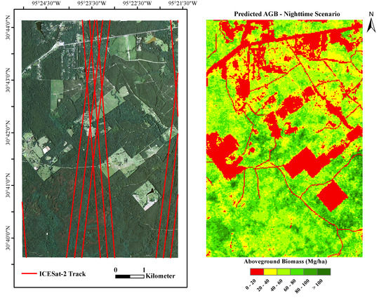
2.1. Study Area

The study was carried out in Sam Houston National Forest (SHNF) located in south-east Texas, USA (Latitude 30°42′N, Longitude 95°23′W). Elevations range from 62 m to 105 m, with an average of 85 m [8]. Approximately 58% of the region or 80% of its forested area (NLCD classes—deciduous forest, evergreen forest, mixed forest, and woody wetland) is classified as evergreen forests [42] and the site is predominated by pine forests, which include Loblolly pine (Pinus taeda) plantations and old growth Loblolly pine stands [8]. The planned ICESat-2 track locations for the first two years of the mission over the study area [31] are depicted in Figure 1.

2.2. Simulated ICESat-2-Estimated AGB

Discrete return lidar data acquired in November 2010 over SHNF with a point density of four points per m2, were used to simulate ICESat-2′s photon-counting lidar (PCL) data. Planned track locations, ICESat-2 footprint generator and simulator were made available by the mission’s Science Team (ST). Footprints spaced 70 cm apart were generated along each planned ICESat-2 track and photons were simulated using the airborne lidar data. A detailed description of the PCL simulation is provided in Neuenschwander and Magruder [14]. To summarize, discrete return lidar points falling within each generated ICESat-2 footprint were used to generate a pseudo-waveform [43], a vector with heights or elevation was then constructed for each footprint, the number of photons based on design cases were randomly determined and random sampling of the height vector weighted by the pseudo-waveform was carried out [14]. The design cases for several land cover types were developed by the ICESat-2 instrument team to support model development for signal prediction [14] (p. 4). As a result, the average number of signal photons per shot was modeled at 1.9, based on the ATLAS performance model for temperate forests [44] and the algorithm returned up to three photons per 14-m diameter footprint.
Anticipated noise photons, representative of solar background noise and effects of atmospheric scattering [45], were added to the simulated dataset. Two datasets were generated to represent the following—(1) daytime scenario with expected noise levels for daytime operation of ICESat-2, and (2) nighttime scenario with noise levels based on night operation of ICESat-2. Popescu et al. [39] devised and applied novel noise filtering and photon classification algorithms to simulated ICESat-2 data and reported average RMSE values of 2.70 m and 3.59 m for estimating canopy heights with nighttime and daytime scenarios respectively. PCL data processing algorithms developed by Popescu et al. [39] were applied to the data to remove noise photons and classify photons into top of canopy points and ground surface elevation points; subtracting the latter from the former yielded tree canopy height values within footprints. Another PCL simulation using above-ground-level heights was carried out and no noise photons were added to the data. In total, data for three scenarios were analyzed; (1) daytime scenario, (2) nighttime scenario, and (3) no noise scenario. Real ICESat-2 data became available on 28th May 2019, but planned tracks will be collected throughout the satellite mission. For a visual comparison, Figure 2 shows real ICESat-2 data and simulated PCL data over similar pine forests in Texas. At the time of this writing, real data was not available over SHNF. The purpose of this visual comparison is to offer insights into the performance of the photon classification and noise removal algorithm with real data, which was used to process the simulated PCL data used for this study. The focus of this study is on developing the use of DL methods with PCL type and structure that will be provided in the near future by the ICESat-2 mission.
Data representative of ICESat-2′s ATL08 product was used for modeling relationships with spatially coincident airborne-lidar derived AGB. To maintain consistency with the ATL08 format, 100 m segments were extracted from the simulated datasets and height percentiles, canopy cover, and canopy density metrics were calculated [38]. The utilization of the simulated ICESat-2 PCL vegetation product for estimating AGB and airborne lidar-derived canopy cover are presented in Narine et al. [38]. To summarize, linear regression models relating simulated PCL metrics for a subset of the segments (n = 85) to airborne lidar-derived AGB were developed and their performance was assessed with a separate test set (n = 36). AGB models yielded RMSEs of 25.35 Mg/ha, 19.23 Mg/ha, and 19.16 Mg/ha and R2 values of 0.63, 0.79, and 0.79 for the daytime scenario, nighttime scenario, and no noise scenario respectively [38].
Using AGB models developed with the simulated PCL vegetation product over SHNF, AGB density (Mg/ha) was estimated for each segment over the study site and applied to 30 m pixels to match Landsat TM pixels, as described in Narine et al. [40]. AGB was assigned based on the portion of a 100 m segment across a pixel and the value was extrapolated to represent the pixel size using the estimated area of a segment across a pixel. Segments less than 7 m in a pixel were excluded from analysis and the average pixel AGB was calculated in instances where there were two segments (parts) of equal lengths traversing a pixel. The steps for assigning AGB density to pixels were repeated for each data scenario using the corresponding prediction equation developed from linear regression analysis. Then, 70% of the data (pixels) was randomly assigned to the training dataset and the remaining 30% was allotted to the test set and used for model evaluation [40]. The training and test sets for each scenario consisted of 1448 and 620 30-m pixels respectively and were the same as data used in Narine et al. [40] in order to facilitate the comparisons of DNN models with the RF approach implemented in that study. The flowchart of steps executed to estimate AGB with simulated ICESat-2 data [38] and achieve wall-to-wall AGB coverage using DNNs, is presented in Figure 3.

2.3. Mapped Predictors

A Landsat 5 Thematic Mapper (TM) cloud-free scene encompassing the study site, from path/row 26/39 and acquired in November, 2010 was downloaded from U.S. Geological Survey (USGS) Earth Explorer in GeoTIFF format and re-projected to UTM, WGS84, Zone 15N. The image was processed in ENVI 5.5 to top-of-atmosphere (TOA) reflectance and vegetation indices were computed. Land cover and canopy cover maps from the 2011 National Land Cover Database (NLCD) [42] were also downloaded and georeferenced in the same projection as the Landsat TM image. The same predictor variables used in Narine et al. [40] were also utilized in this study. Consequently, the six predictor variables used for AGB modeling were:
  • Spectral Metrics from Landsat 5 TM-
    Normalized Difference Vegetation Index (NDVI): (NIR − Red)/(NIR + Red)
    Enhanced Vegetation Index (EVI): 2.5 * ((NIR − Red)/(NIR + 6 * Red − 7.5 * Blue + 1))
    Soil Adjusted Vegetation Index (SAVI): ((NIR − Red)/(NIR + Red + 0.5)) * (1.5)
    Modified Soil Adjusted Vegetation Index (MSAVI): (2 * NIR + 1 − sqrt ((2 * NIR + 1)² − 8 * (NIR − Red)))/2
  • NLCD 2011 land cover map
  • NLCD 2011 US Forest Service tree canopy cover
With the potential to highlight vegetation changes during the start and end of the growing season, the Landsat-derived NDVI is an important indicator that has demonstrated promise for monitoring vegetation phenology across time and at regional scales [46]. To examine the impact on model performance, one year of Landsat imagery, from 1st May 2010 to 30th April 2011, were downloaded from USGS Earth Explorer and processed as before. The same Landsat-based vegetation metrics were calculated for each processed image, then combined with land cover and tree canopy cover and used for biomass prediction, resulting in an extended dataset containing a total of 94 variables. The extended dataset was used to develop a second set of models for each scenario following the methods described in Section 2.4., and the results were compared with models that utilized single-date imagery.

2.4. Deep Neural Networks (DNNs)

DL via neural networks is comprised of stacked layers that facilitate learning via successive layers of representations of the input data [47] (p. 8). Essentially, a layer transforms the data, as specified by weights, which are referred to as the parameters of the layer [47]. The process of learning entails finding the optimum values of the weights in each layer of a neural network, which are adjusted by an optimizer, based on the loss score. A loss function measures the difference between the observed values and predictions from the neural network and adjustments with the optimizer serves to lower the loss score [47]. The network weights are randomly initialized resulting in a high loss score but are adjusted as each example (batch) is processed and iterated several times to produce weights that lower the loss function [47] (p. 11). Essentially, the gradient of the loss, given the combination of the weights, is computed and the parameters are subsequently moved to an extent defined by the learning rate, to reduce the loss for the batch [47]. In terms of optimization, there are several methods of reducing loss through gradient descent to improve network accuracy. An activation function can also be added to each layer in the model, enabling the layer to learn non-linear transformations of the data. In this study, modeling was done with Keras [47] with TensorFlow backend in R and data visualization, with ArcGIS 10.4 software. For all neural network architectures developed, the Root Mean Square Propagation (RMSProp) optimizer and rectified linear unit (ReLU) as the activation function, which are regarded as good options for different tasks [47], were used. The activation function g is applied element-wise defined by the function g ( z ) = m a x { 0 ,   z } [30,48]. Assuming h is a vector of hidden units in a layer, then h = g ( W T x + c ) , where W are the weights of the transformation and c are the biases [48] (p. 168), such that each element in the hidden layer has a different weight and bias parameter [49]. For all models, the loss function was defined with the mean squared error (MSE), the learning rate was initially set to 0.001, and epochs and batch size were 100 and 32 respectively.
In terms of network topology, the first set of neural network models consisted of one input layer with 6 neurons (one for each predictor) and one output node for the predicted AGB, and the second set of models consisted of 94 neurons in the input layer. A primary task was to find the number of neurons in the hidden layer and the number of hidden layers between the input and output layers. The architecture of a neural network, specifically, the number of hidden layers and nodes are critical [50] since this affects the ability to learn the data [49] and ultimately impacts the network’s predictive capacity. A trial and error approach is common for determining network topology, while studies have presented techniques for identifying an optimal network structure for specific applications. For example, Doukim et al. [50] highlighted a course to fine search technique for determining the number of hidden neurons in a multi-layer perceptron (feedforward) neural network for skin detection from images. Doukim et al. [50] used a binary search, with hidden neurons set to 1, 2, 4, 8, 16, 32, 64, and 128 and then a sequential search around a specific range indicated by the binary search to fine-tune the process of finding the number of hidden neurons that resulted in the smallest MSE. In this study, a network structure consisting of 112 hidden neurons was used to construct a neural network for skin detection. In another study, Guang-Bin [51] demonstrated that a two layer feedforward neural network is sufficient for learning with minimal error and suggests that the number of nodes in the first layer is given by:
( m + 2 ) N + 2 N / ( m + 2 )
And the number of hidden nodes in the second layer is defined by:
m N / ( m + 2 )
where N is the number of samples and m is the number of output neurons.
For comparison purposes, the equations for determining the number of hidden nodes in the first and second hidden layers proposed by Guang-Bin [51] were applied to the training dataset, which equates to a neural network with 98 neurons in the first layer and 20 hidden nodes in the second layer. However, since determining the optimum network structure was crucial in order to understand the applicability of deep architectures with simulated ICESat-2 data, the number of hidden neurons and layers were also varied. Exploratory analysis involving gradual increases in the number of hidden neurons in the first hidden layer (e.g., binary search in Doukim et al. [50]) did not result in substantial changes in model performance. As a result, the number of neurons were varied in intervals of 20 up to 200 neurons and then in intervals of 100 with a maximum of 1000 hidden neurons in the first hidden layer. The results from the application of each trained model to the separate test set were compared using the RMSE and R2 values. Guang-Bin [51] proposed a neural network architecture consisting of a large first hidden layer and a second hidden layer that is considerably narrower. To adopt this feature to the network architecture for deeper models, successively narrow layers were applied. A second hidden layer was added to the neural network that gave the highest R2 and lowest RMSE value in each scenario and the number of neurons was varied in increments of 20 up to the number of hidden neurons in the previous layer. Layers were added until there were no further improvements in model performance.
With the final selected network structure for each scenario, the learning rate used by the RMSProp optimizer was changed from 0.001 to 0.1, 0.01, and 0.0001 [52] and model performance with the test set were compared for each hyperparameter setting. Regarded as the most important hyperparameter of DL algorithms [48] (p. 424), the learning rate affects the model’s capacity, as indicated by the model error. Too large to too small learning rates could increase training error as well as training times in the case where rates are too small and sub-optimal. Final models yielding the lowest RMSE and highest R2 for each scenario were used to generate AGB maps. Results were compared with RF models [40] for the three data scenarios and new RF models were developed with the extended dataset consisting of 94 predictors for comparisons with final DNN models generated with the same data. Consistent with the implementation of RF described in Narine et al. [40], models were developed with the ModelMap R package.

3. Results

An assessment of the first set of neural networks with six variables predicting simulated PCL-estimated AGB for the daytime, nighttime, and no noise data scenarios, indicated models with 300 hidden neurons, 600 hidden neurons, and 500 hidden neurons in the first hidden layer performed best (Table 1). These models explained 40%, 47%, and 48% of the variance in simulated PCL-estimated AGB with RMSEs of 19.90 Mg/ha, 19.72 Mg/ha, and 20.29 Mg/ha for the daytime, nighttime, and no noise scenarios respectively. Incremental increases in the number of neurons in the first hidden layer yielded R2 values ranging from 0.38 to 0.40, 0.45 to 0.47, and 0.46 to 0.48 with the daytime, nighttime, and no noise scenarios. In comparison, using the formula proposed by Guang-Bin [51], a DNN with 98 neurons in the first layer and 20 hidden nodes in the second layer yielded a R2 and RMSE of 0.40 and 19.92 Mg/ha, 0.45 and 19.95 Mg/ha, and 0.47 and 20.27 Mg/ha for the daytime, nighttime, and no noise scenarios respectively.
To better understand the applicability of DNNs using simulated PCL-estimated AGB and predictors consisting of Landsat spectral metrics, land cover and canopy cover, model performance from varying the number of hidden neurons in each additional hidden layer were assessed and compared. With the daytime scenario, a second hidden layer was added and the neurons were increased in increments of 20 to a maximum of 300 hidden neurons. The DNN consisting of 160 neurons in the second hidden layer performed best, in terms of R2 and RMSE but the addition of a third hidden layer did not improve model performance (Figure 4). With the nighttime scenario, a second hidden layer with hidden neurons varied from 20 to 500 was investigated, leading to a DNN structure consisting of two hidden layers with 600 in the first hidden layer and 400 in the second. The lowest reported RMSE corresponding to the DNN with a third hidden layer is shown in Figure 4. However, a DNN with two hidden layers achieved the best results. The best performing model with the no noise scenario consisted of five densely connected layers; one input layer, three hidden layers with 500, 300, and 60 neurons in the first, second, and third hidden layers respectively, and one output layer. The DNNs with four hidden layers did not result in better models (Figure 4).
Findings from tuning the learning rate for each DNN (Table 2) resulted in models with the parameter set to 0.0001 for the daytime and nighttime scenarios and 0.001 for the no noise scenario. Substantial decreases in R2 were noted when the learning rate was increased to 0.01 and 0.1 indicating an overall suitability of the 0.001 and 0.0001 level with the data. For example, with the DNN model for the daytime scenario, the learning rate that was set to 0.0001 yielded the highest R2 and lowest RMSE of 0.42 and 19.55 Mg/ha, while a learning rate of 0.1 resulted in a R2 of 0.25 and RMSE of 22.32 Mg/ha. With the nighttime scenario, a change in the learning rate from 0.1 to 0.0001 increased the R2 value from 0.34 to 0.49. The model for the no noise scenario yielded a R2 and RMSE of 0.50 and 19.82 Mg/ha when the learning rate was set to 0.001 or 0.0001, compared to 0.40 and 21.66 Mg/ha when the rate was 0.1.
Scatterplots with simulated PCL-estimated AGB vs DNN predicted AGB (Figure 5) show the line of best fit adjacent to the 1:1 line. However, the DNN models tended to underestimate AGB, where this trend was most pronounced with the daytime scenario and least prominent with the no noise scenario.
Models developed with the extended dataset consisting of 94 predictor variables, yielded substantially better results and a comparison of DNN models with RF models produced with the same data highlighted comparable predictive abilities (Table 3). Except for the no noise scenario, the R2 values were identical to RF models with six predictors [40] as well as models with 94 predictors and the RMSEs were in the same range. In terms of DNNs, the R2 increased from 0.42 (p-value < 0.001), 0.49 (p-value < 0.001), and 0.50 (p-value < 0.001), to 0.64 (p-value < 0.001), 0.66 (p-value < 0.001), and 0.67 (p-value < 0.001) for the daytime, nighttime, and no noise scenarios respectively. The RMSEs improved from 19.55 Mg/ha to 15.47 Mg/ha, 19.35 Mg/ha to 15.64 Mg/ha, and 19.82 Mg/ha to 16.09 Mg/ha with daytime, nighttime, and no noise scenarios respectively. The final neural network model for the daytime scenario consisted of 500 neurons in the first hidden layer and 160 neurons in the second layer. The regression model for the nighttime scenario also used two hidden layers with 300 and 200 neurons in the first and second layer respectively while the final NN structure for the no noise scenario consisted of one hidden layer with 500 neurons. For all the scenarios, a learning rate of 0.001 yielded the best results.
Wall-to-wall AGB predictions were obtained from the final DNN models with 94 predictor variables for each data scenario. The average AGB predictions from maps (Figure 6, Figure 7 and Figure 8) produced with the trained DNN models for the daytime, nighttime, and no noise scenarios were 39.90 Mg/ha, 42.93 Mg/ha, and 44.78 Mg/ha respectively. Overall, the AGB maps correspond with vegetation patterns in the study area with the southern portion of the site predominated by forests, primarily mature pines, and lower AGB values in northern portions, which includes young pine stands. Higher AGB values are evident in the map generated with the no noise scenario while lower AGB ranges are more prevalent with the map for the daytime scenario. Maximum predicted AGB density for 30 m cells was 125.86 Mg/ha for the daytime scenario, 123.83 Mg/ha with the nighttime scenario, and 127.93 Mg/ha with the no noise scenario. With the training data, average AGB were 51.21 Mg/ha, 52.24 Mg/ha, and 52.09 Mg/ha for the daytime, nighttime, and no noise scenarios respectively and the maximum values were 139.61 Mg/ha, 119.75 Mg/ha, and 150.64 Mg/ha respectively.

4. Discussion

With ICESat-2 already in operation, data will be available for meeting the mission’s science objectives, one of which has a direct benefit to the ecosystem community [11]. The mission’s ATL08 product will provide canopy heights and canopy cover which will be used to produce global maps of these attributes at the end of the mission [11,31]. The investigation of approaches for utilizing ICESat-2 data using simulated data could potentially offer a better understanding of how the data can be used for vegetation studies, provide insights about the expected accuracies of techniques examined, and potentially facilitate quick adoption using actual data. The relationship between simulated PCL metrics from 100 m segments and reference airborne lidar-estimated AGB along ICESat-2 profiles over the study site in SHNF was modeled in a previous study [38] and the resulting prediction equations were applied to estimate AGB for the daytime, nighttime, and no noise scenarios. Using freely available data, including satellite data, which offers global coverage, AGB estimates were up-scaled from 3% of 30 m pixels which comprise the area, to produce spatially explicit AGB coverage.
In this study, simulated PCL estimated AGB along two years of tracks over the study site were used in synergy with spectral metrics derived from Landsat imagery and NLCD products to develop regression-based, feed-forward neural network models for application to the rest of the study site. Using six predictor variables, the final model for the daytime scenario consisted of four densely connected layers; one input layer, two hidden layers, and one output layer. With the nighttime scenario, the neural network consisted of two non-linear hidden layers and the neural network structure for the no noise scenario consisted of three hidden layers. These neural networks used fully connecting layers and at least 300 neurons in the first hidden layer of each model, resulting in architectures with hundreds of thousands of parameters or weights. Increasing the width of the neural networks led to some improvements in terms of RMSEs with negligible differences in training time and with added depth, the model performance improved with consistently better results from the nighttime scenario than daytime scenario. One possible reason for the R2 values being less than expected could be dissimilarities in the range of biomass represented in the test data and training data, as mentioned in a biomass mapping study with neural networks by Foody et al. [53]. With more training data, the use of a deeper architecture could be beneficial and likely improve results [35]. Another consideration is the grid size chosen for upscaling AGB estimates to obtain spatially complete coverage, where aggregating AGB to larger grid sizes may improve the relationships with predictors from optical satellite data. For example, Li et al. [54] used lidar-derived height metrics to estimate AGB and then combined lidar-derived estimates with vegetation indices from satellite imagery for regional AGB mapping. A comparison of lidar-derived AGB and vegetation indices at different spatial resolutions, specifically at 250 m, 500 m, and 1000 m emphasized higher correlations at coarser spatial resolution. Li et al. [54] indicated that the increased correlation between lidar-derived AGB and vegetation indices at the coarser resolutions were possibly due to minimization of the effects of spatial heterogeneity.
While additional training data representative of the range of AGB, including data in the test set, may improve model accuracies, it is important to note that considerable improvements in model performance were achieved with the integration of data from a year of Landsat imagery. Vegetation indices, particularly EVI and NDVI, from repeat imagery facilitate the extraction of important phenological information [46,55]. With the use of Landsat images acquired every 16 days, computed vegetation indices from each may capture seasonal vegetation trends and as the results indicate, demonstrate promise for estimating AGB with simulated ICESat-2 data. With free and open access to Landsat imagery and given the available resolution, the data could potentially be used for achieving spatially comprehensive coverage of forest biophysical parameters with real ICESat-2 data. In terms of model structure with the extended dataset, the final models consisted of two hidden layers for the daytime and nighttime scenarios and one hidden layer with 500 neurons for the no noise scenario. Additional layers of representation to the final selected network structures did not improve model performance and the findings demonstrate that the DNN models for all the data scenarios yielded results that were comparable to RF models.
A comparison of different learning rates for selected model structures revealed apparent differences in reported R2 values and RMSEs. In one study, comparison of learning rates using a regression-based, deep auto-encoder model with two hidden layers for gene expression prediction yielded MSEs ranging from 0.289 to 0.292, with the best results attributed to the model with the highest learning rate; 0.1 [52]. The learning rates investigated were 0.1, 0.01, 0.001, 0.0001, and 0.00001. Conversely, findings from this study emphasized the importance of the lowest learning rates investigated (0.001 and 0.0001) for predicting AGB in each data scenario and with highest RMSE and lowest R2 values corresponding to DNNs when the learning rates were set to 0.1.
The use of RF has been successfully demonstrated in the literature for mapping AGB with data from ICESat-2′s predecessor [4], but with the ability to handle large, complex datasets, DL algorithms could be explored for generating a spatially explicit AGB product from an integration of multi-source data, including GEDI, ICESat-2, satellite optical imagery, and radar data with other ancillary data. For instance, a combination of predicted AGB density from GEDI and ICESat-2 data could be combined with mapped variables derived from Landsat data, for generating a wall-to-wall AGB map. With current and upcoming space-based vegetation missions like NASA-ISRO Synthetic Aperture Radar (NISAR) [56] and the European Space Agency P-band radar BIOMASS mission [57], the volume of data that can potentially provide rich insights about the world’s forests will grow considerably and DL models could play a larger role in predicting forest attributes. Given new data from satellite sensors and multiple, open-source DL frameworks (e.g., TensorFlow), DL architectures for predicting AGB can be explored more extensively. Future work could entail an examination and comparison of multiple DL techniques, like the stacked sparse auto-encoder model [15], autoregressive neural network [58], and recurrent neural network [59], for producing a wall-to-wall AGB product with ICESat-2 and other satellite remote sensing data. Finally, limited examples of DL models for estimating forest biophysical parameters in the literature suggest the need for further research to better understand or identify potential benefits from DL for forest mapping applications.

5. Conclusions

In this study, an approach for mapping AGB was developed by integrating simulated PCL-estimated AGB with Landsat imagery, NLCD canopy cover, and land cover using DNNs. The effect of network structure and learning rate on model performance were evident with the latter having sizeable impacts on the reported error metrics. Noteworthy is the substantial improvements in biomass prediction models from using one year of Landsat data. Given the continuity of Landsat and available resolution for deriving valuable vegetation metrics every 16 days, the data could be leveraged to characterize vegetation and better understand phenological trends over large areas. Findings with simulated PCL-estimated data along ICESat-2 profiles, especially with the nighttime scenario (R2 = 0.66), highlight the potential for generating a wall-to-wall AGB product with ICESat-2 by adopting a synergistic approach with Landsat optical imagery, canopy cover, and land cover. With limited examples of DL models for estimating forest biophysical parameters and given the growing volumes of data from current space lidars and upcoming satellite missions and given the learning capacity of DL, DL algorithms could be explored further in future research. In doing so, multiple techniques for modeling AGB and other forest structural parameters could be implemented and compared.

Author Contributions

Conceptualization, S.C.P., L.L.N.; methodology, L.L.N. and S.C.P.; formal analysis, L.L.N.; investigation, L.L.N. and L.M.; resources, S.C.P.; writing—original draft preparation, L.L.N.; writing—review and editing, L.L.N. and S.C.P.; visualization, L.L.N. and L.M.; supervision, S.C.P.; funding acquisition, S.C.P.

Funding

This work was supported by NASA under Grant Number NNX15AD02G.

Acknowledgments

We greatly appreciate the support provided by NASA and very thankful for the constructive comments from reviewers.

Conflicts of Interest

The authors declare no conflict of interest.

References

  1. Hall, F.G.; Bergen, K.; Blair, J.B.; Dubayah, R.; Houghton, R.; Hurtt, G.; Kellndorfer, J.; Lefsky, M.; Ranson, J.; Saatchi, S.; et al. Characterizing 3D vegetation structure from space: Mission requirements. Remote Sens. Environ. 2011, 115, 2753–2775. [Google Scholar] [CrossRef] [Green Version]
  2. Zald, H.S.J.; Wulder, M.A.; White, J.C.; Hilker, T.; Hermosilla, T.; Hobart, G.W.; Coops, N.C. Integrating Landsat pixel composites and change metrics with lidar plots to predictively map forest structure and aboveground biomass in Saskatchewan, Canada. Remote Sens. Environ. 2016, 176, 188–201. [Google Scholar] [CrossRef] [Green Version]
  3. Goetz, S.; Dubayah, R. Advances in remote sensing technology and implications for measuring and monitoring forest carbon stocks and change. Carbon Manag. 2011, 2, 231–244. [Google Scholar] [CrossRef]
  4. Chi, H.; Sun, G.Q.; Huang, J.L.; Guo, Z.F.; Ni, W.J.; Fu, A.M. National Forest Aboveground Biomass Mapping from ICESat/GLAS Data and MODIS Imagery in China. Remote Sens. 2015, 7, 5534–5564. [Google Scholar] [CrossRef] [Green Version]
  5. Hu, T.; Su, Y.; Xue, B.; Liu, J.; Zhao, X.; Fang, J.; Guo, Q. Mapping Global Forest Aboveground Biomass with Spaceborne LiDAR, Optical Imagery, and Forest Inventory Data. Remote Sens. 2016, 8, 565. [Google Scholar] [CrossRef]
  6. Nelson, R.; Margolis, H.; Montesano, P.; Sun, G.; Cook, B.; Corp, L.; Andersen, H.-E.; deJong, B.; Pellat, F.P.; Fickel, T.; et al. Lidar-based estimates of aboveground biomass in the continental US and Mexico using ground, airborne, and satellite observations. Remote Sens. Environ. 2017, 188, 127–140. [Google Scholar] [CrossRef] [Green Version]
  7. Glenn, N.F.; Neuenschwander, A.; Vierling, L.A.; Spaete, L.; Li, A.H.; Shinneman, D.J.; Pilliod, D.S.; Arkle, R.S.; McIlroy, S.K. Landsat 8 and ICESat-2: Performance and potential synergies for quantifying dryland ecosystem vegetation cover and biomass. Remote Sens. Environ. 2016, 185, 233–242. [Google Scholar] [CrossRef]
  8. Popescu, S.C. Estimating biomass of individual pine trees using airborne lidar. Biomass Bioenergy 2007, 31, 646–655. [Google Scholar] [CrossRef]
  9. Neuenschwander, A.; Pitts, K. The ATL08 land and vegetation product for the ICESat-2 Mission. Remote Sens. Environ. 2019, 221, 247–259. [Google Scholar] [CrossRef]
  10. Stysley, P.R.; Coyle, D.B.; Clarke, G.B.; Frese, E.; Blalock, G.; Morey, P.; Kay, R.B.; Poulios, D.; Hersh, M. Laser Production for NASA’s Global Ecosystem Dynamics Investigation (GEDI) Lidar. In Proceedings of the Conference on Laser Radar Technology and Applications XXI, Baltimore, MD, USA, 19–20 April 2016. [Google Scholar]
  11. Markus, T.; Neumann, T.; Martino, A.; Abdalati, W.; Brunt, K.; Csatho, B.; Farrell, S.; Fricker, H.; Gardner, A.; Harding, D.; et al. The Ice, Cloud, and land Elevation Satellite-2 (ICESat-2): Science requirements, concept, and implementation. Remote Sens. Environ. 2017, 190, 260–273. [Google Scholar] [CrossRef]
  12. Marselis, S.; Armston, J.; Dubayah, R. Summary of the Second GEDI Science Team Meeting. Earth Obs. 2016, 6, 31–36. [Google Scholar]
  13. Sun, X. Space-Based Lidar Systems. In Proceedings of the Conference on Lasers and Electro-Optics 2012, San Jose, CA, USA, 6–11 May 2012. [Google Scholar]
  14. Neuenschwander, A.L.; Magruder, L.A. The Potential Impact of Vertical Sampling Uncertainty on ICESat-2/ATLAS Terrain and Canopy Height Retrievals for Multiple Ecosystems. Remote Sens. 2016, 8, 16. [Google Scholar] [CrossRef]
  15. Shao, Z.F.; Zhang, L.J.; Wang, L. Stacked Sparse Autoencoder Modeling Using the Synergy of Airborne LiDAR and Satellite Optical and SAR Data to Map Forest Above-Ground Biomass. IEEE J. Sel. Top. Appl. Earth Obs. Remote Sens. 2017, 10, 5569–5582. [Google Scholar] [CrossRef]
  16. Lu, D.S.; Chen, Q.; Wang, G.X.; Liu, L.J.; Li, G.Y.; Moran, E. A survey of remote sensing-based aboveground biomass estimation methods in forest ecosystems. Int. J. Digit. Earth 2016, 9, 63–105. [Google Scholar] [CrossRef]
  17. Popescu, S.C.; Zhao, K.; Neuenschwander, A.; Lin, C. Satellite lidar vs. small footprint airborne lidar: Comparing the accuracy of aboveground biomass estimates and forest structure metrics at footprint level. Remote Sens. Environ. 2011, 115, 2786–2797. [Google Scholar] [CrossRef]
  18. Lefsky, M.A. A global forest canopy height map from the Moderate Resolution Imaging Spectroradiometer and the Geoscience Laser Altimeter System. Geophys. Res. Lett. 2010, 37, 5. [Google Scholar] [CrossRef]
  19. Simard, M.; Pinto, N.; Fisher, J.B.; Baccini, A. Mapping forest canopy height globally with spaceborne lidar. J. Geophys. Res. Biogeosci. 2011, 116, 12. [Google Scholar] [CrossRef]
  20. Breiman, L. Random forests. Mach. Learn. 2001, 45, 5–32. [Google Scholar] [CrossRef]
  21. Baccini, A.; Friedl, M.A.; Woodcock, C.E.; Warbington, R. Forest biomass estimation over regional scales using multisource data. Geophys. Res. Lett. 2004, 31, 4. [Google Scholar] [CrossRef]
  22. Garcia-Gutierrez, J.; Martinez-Alvarez, F.; Troncoso, A.; Riquelme, J.C. A comparison of machine learning regression techniques for LiDAR-derived estimation of forest variables. Neurocomputing 2015, 167, 24–31. [Google Scholar] [CrossRef]
  23. Tian, X.; Li, Z.; Su, Z.; Chen, E.; van der Tol, C.; Li, X.; Guo, Y.; Li, L.; Ling, F. Estimating montane forest above-ground biomass in the upper reaches of the Heihe River Basin using Landsat-TM data. Int. J. Remote Sens. 2014, 35, 7339–7362. [Google Scholar] [CrossRef] [Green Version]
  24. Wang, L.; Liu, J.P.; Xu, S.H.; Dong, J.J.; Yang, Y. Forest Above Ground Biomass Estimation from Remotely Sensed Imagery in the Mount Tai Area Using the RBF ANN Algorithm. Intell. Autom. Soft Comput. 2018, 24, 391–398. [Google Scholar] [CrossRef]
  25. Hatcher, W.G.; Yu, W. A Survey of Deep Learning: Platforms, Applications and Emerging Rlesearch Trends. IEEE Access 2018, 6, 24411–24432. [Google Scholar] [CrossRef]
  26. Lv, J.J.; Zhang, B.; Li, X.Q. Research on Object Detection Algorithm Based on PVANet. Adv. Comput. Commun. Comput. Sci. 2019, 759, 141–151. [Google Scholar] [CrossRef]
  27. Shafaey, M.A.; Salem, M.A.M.; Ebied, H.M.; Al-Berry, M.N.; Tolba, M.F. Deep Learning for Satellite Image Classification; Springer Nature: Basel, Switzerland, 2019. [Google Scholar]
  28. Zhu, X.X.; Tuia, D.; Mou, L.C.; Xia, G.S.; Zhang, L.P.; Xu, F.; Fraundorfer, F. Deep Learning in Remote Sensing. IEEE Geosci. Remote Sens. Mag. 2017, 5, 8–36. [Google Scholar] [CrossRef]
  29. Garcia-Gutierrez, J.; Gonzalez-Ferreiro, E.; Mateos-Garcia, D.; Riquelme-Santos, J.C. A Preliminary Study of the Suitability of Deep Learning to Improve LiDAR-Derived Biomass Estimation. Hybrid. Artif. Intell. Syst. 2016, 9648, 588–596. [Google Scholar] [CrossRef]
  30. Trier, O.D.; Salberg, A.B.; Kermit, M.; Rudjord, O.; Gobakken, T.; Naesset, E.; Aarsten, D. Tree species classification in Norway from airborne hyperspectral and airborne laser scanning data. Eur. J. Remote Sens. 2018, 51, 336–351. [Google Scholar] [CrossRef]
  31. Neuenschwander, A.; Popescu, S.; Nelson, R.; Harding, D.; Pitts, K.; Pederson, D.; Sheridan, R. ICE, CLOUD, and Land Elevation Satellite (ICESat-2) Algorithm Theoretical Basis Document (ATBD) for Land —Vegetation Along-track products (ATL08). Available online: https://go.nasa.gov/31PqmKp (accessed on 24 June 2019).
  32. Baghdadi, N.; le Maire, G.; Fayad, I.; Bailly, J.S.; Nouvellon, Y.; Lemos, C.; Hakamada, R. Estimation of Forest Height and Aboveground Biomass from ICESat-2/GLAS Data in Eucaluptus Plantations in Brazil. In Proceedings of the 2014 IEEE Geoscience and Remote Sensing Symposium, Quebec City, QC, Canada, 13–18 July 2014; pp. 725–728. [Google Scholar] [CrossRef]
  33. Harding, D.J.; Carabajal, C.C. ICESat waveform measurements of within-footprint topographic relief and vegetation vertical structure. Geophys. Res. Lett. 2005, 32, 4. [Google Scholar] [CrossRef]
  34. Lefsky, M.A.; Keller, M.; Pang, Y.; de Camargo, P.B.; Hunter, M.O. Revised method for forest canopy height estimation from Geoscience Laser Altimeter System waveforms. J. Appl. Remote Sens. 2007, 1, 18. [Google Scholar] [CrossRef]
  35. Liu, K.; Wang, J.; Zeng, W.; Song, J. Comparison and Evaluation of Three Methods for Estimating Forest above Ground Biomass Using TM and GLAS Data. Remote Sens. 2017, 9, 341. [Google Scholar] [CrossRef]
  36. Gwenzi, D.; Lefsky, M.A.; Suchdeo, V.P.; Harding, D.J. Prospects of the ICESat-2 laser altimetry mission for savanna ecosystem structural studies based on airborne simulation data. ISPRS J. Photogramm. Remote Sens. 2016, 118, 68–82. [Google Scholar] [CrossRef]
  37. Montesano, P.M.; Rosette, J.; Sun, G.; North, P.; Nelson, R.F.; Dubayah, R.O.; Ranson, K.J.; Kharuk, V. The uncertainty of biomass estimates from modeled ICESat-2 returns across a boreal forest gradient. Remote Sens. Environ. 2015, 158, 95–109. [Google Scholar] [CrossRef]
  38. Narine, L.L.; Popescu, S.; Neuenschwander, A.; Zhou, T.; Srinivasan, S.; Harbeck, K. Estimating aboveground biomass and forest canopy cover with simulated ICESat-2 data. Remote Sens. Environ. 2019, 224, 1–11. [Google Scholar] [CrossRef]
  39. Popescu, S.C.; Zhou, T.; Nelson, R.; Neuenschwander, A.; Sheridan, R.; Narine, L.; Walsh, K.M. Photon counting LiDAR: An adaptive ground and canopy height retrieval algorithm for ICESat-2 data. Remote Sens. Environ. 2018, 208, 154–170. [Google Scholar] [CrossRef]
  40. Narine, L.L.; Popescu, S.; Zhou, T.; Srinivasan, S.; Harbeck, K. Mapping forest aboveground biomass with a simulated ICESat-2 vegetation canopy product and Landsat data. Ann. For. Res. 2019, 62. [Google Scholar] [CrossRef]
  41. Stathakis, D. How many hidden layers and nodes? AU—Stathakis, D. Int. J. Remote Sens. 2009, 30, 2133–2147. [Google Scholar] [CrossRef]
  42. Homer, C.; Dewitz, J.; Yang, L.M.; Jin, S.; Danielson, P.; Xian, G.; Coulston, J.; Herold, N.; Wickham, J.; Megown, K. Completion of the 2011 National Land Cover Database for the Conterminous United States—Representing a Decade of Land Cover Change Information. Photogramm. Eng. Remote Sens. 2015, 81, 345–354. [Google Scholar] [CrossRef]
  43. Blair, J.B.; Hofton, M.A. Modeling laser altimeter return waveforms over complex vegetation using high-resolution elevation data. Geophys. Res. Lett. 1999, 26, 2509–2512. [Google Scholar] [CrossRef]
  44. Martino, A. ATLAS Performance Spreadsheet. Available online: http://icesat.gsfc.nasa.gov/icesat2/data/sigma/sigma_data.php (accessed on 4 June 2018).
  45. Moussavi, M.S.; Abdalati, W.; Scambos, T.; Neuenschwander, A. Applicability of an automatic surface detection approach to micropulse photon-counting lidar altimetry data: Implications for canopy height retrieval from future ICESat-2 data. Int. J. Remote Sens. 2014, 35, 5263–5279. [Google Scholar] [CrossRef]
  46. Snyder, K.A.; Huntington, J.L.; Wehan, B.L.; Morton, C.G.; Stringham, T.K. Comparison of Landsat and Land-Based Phenology Camera Normalized Difference Vegetation Index (NDVI) for Dominant Plant Communities in the Great Basin. Sensors 2019, 19, 1139. [Google Scholar] [CrossRef]
  47. Chollet, F. Deep Learning with Python; Manning Publications Co.: New York, NY, USA, 2018. [Google Scholar]
  48. Goodfellow, I.; Bengio, Y.; Courville, A. Deep Learning; MIT Press: Cambridge, MA, USA, 2016; p. 781. [Google Scholar]
  49. Bengio, Y. Learning Deep Architectures for AI; Now Publishers Inc.: Hanover, MA, USA, 2009; Volume 2, pp. 1–55. [Google Scholar]
  50. Doukim, C.A.; Dargham, J.A.; Chekima, A. Finding the number of hidden neurons for an MLP neural network using coarse to fine search technique. In Proceedings of the 10th International Conference on Information Science, Signal Processing and their Applications (ISSPA 2010), Kuala Lumpur, Malaysia, 10–13 May 2010; pp. 606–609. [Google Scholar]
  51. Guang-Bin, H. Learning capability and storage capacity of two-hidden-layer feedforward networks. IEEE Trans. Neural Netw. 2003, 14, 274–281. [Google Scholar] [CrossRef] [PubMed]
  52. Xie, R.; Wen, J.; Quitadamo, A.; Cheng, J.L.; Shi, X.H. A deep auto-encoder model for gene expression prediction. BMC Genom. 2017, 18, 39–49. [Google Scholar] [CrossRef] [PubMed] [Green Version]
  53. Foody, G.M.; Cutler, M.E.; McMorrow, J.; Pelz, D.; Tangki, H.; Boyd, D.S.; Douglas, I. Mapping the biomass of Bornean tropical rain forest from remotely sensed data. Glob. Ecol. Biogeogr. 2001, 10, 379–387. [Google Scholar] [CrossRef]
  54. Li, L.; Guo, Q.H.; Tao, S.L.; Kelly, M.G.; Xu, G.C. Lidar with multi-temporal MODIS provide a means to upscale predictions of forest biomass. Isprs J. Photogramm. Remote Sens. 2015, 102, 198–208. [Google Scholar] [CrossRef]
  55. Ikasari, I.H.; Ayumi, V.; Fanany, M.I.; Mulyono, S. Multiple Regularizations Deep Learning for Paddy Growth Stages Classification from LANDSAT-8. In Proceedings of the 2016 International Conference on Advanced Computer Science and Information Systems, Malang, Indonesia, 15–16 October 2016; IEEE: New York, NY, USA, 2016; pp. 512–517. [Google Scholar]
  56. Rosen, P.; Hensley, S.; Shaffer, S.; Edelstein, W.; Kim, Y.; Kumar, R.; Misra, T.; Bhan, R.; Satish, R.; Sagi, R.; et al. An update on the NASA-ISRO dual-frequency DBF SAR (NISAR) Mission. In Proceedings of the 2016 IEEE International Geoscience and Remote Sensing Symposium (IGARSS), Beijing, China, 10–15 July 2016; pp. 2106–2108. [Google Scholar] [CrossRef]
  57. Carreiras, J.M.B.; Shaun, Q.G.; Toan, T.L.; Minh, D.H.T.; Saatchi, S.S.; Carvalhais, N.; Reichstein, M.; Scipal, K. Coverage of high biomass forests by the ESA BIOMASS mission under defense restrictions. Remote Sens. Environ. 2017, 196, 154–162. [Google Scholar] [CrossRef]
  58. Nunez, R.A.C.; de la Pena, M.; Irigollen, A.F.; Rodriguez, M.R. Deep learning models for the prediction of small-scale fisheries catches: Finfish fishery in the region of “Bahia Magadalena-Almejas”. ICES J. Mar. Sci. 2018, 75, 2088–2096. [Google Scholar] [CrossRef]
  59. Lee, S.; Lee, D. Improved Prediction of Harmful Algal Blooms in Four Major South Korea’s Rivers Using Deep Learning Models. Int. J. Environ. Res. Public Health 2018, 15, 15. [Google Scholar] [CrossRef] [PubMed]
Figure 1. ICESat-2 tract locations overlaid on 2010 National Agriculture Imagery Program (NAIP) aerial imagery within SHNF, Texas (inset map, upper left corner).
Remotesensing 11 01503 g001
Figure 2. (a) Actual ICESat-2 data over pine forests in Texas; (b) Filtered and classified ICESat-2 data over pine forests in Texas; (c) Filtered and classified simulated ICESat-2 data in SHNF.
Remotesensing 11 01503 g002
Figure 3. Workflow for mapping AGB using simulated ICESat-2 and Landsat data.
Remotesensing 11 01503 g003
Figure 4. Neural network structures for predicting AGB with the daytime, nighttime, and no noise scenarios.
Remotesensing 11 01503 g004
Figure 5. (a) Simulated PCL AGB estimated from linear regression vs DNN predicted AGB with test data for the daytime scenario; (b) Simulated PCL AGB estimated from linear regression vs DNN predicted AGB with test data for the nighttime scenario (c) Simulated PCL AGB estimated from linear regression vs DNN predicted AGB with test data for the no noise scenario. The dashed line in each graph is the 1:1 line.
Remotesensing 11 01503 g005
Figure 6. DNN predictions of AGB density at a 30 m spatial resolution for the daytime scenario.
Remotesensing 11 01503 g006
Figure 7. DNN predictions of AGB density at a 30 m spatial resolution for the nighttime scenario.
Remotesensing 11 01503 g007
Figure 8. DNN predictions of AGB density at a 30 m spatial resolution for the no noise scenario.
Remotesensing 11 01503 g008
Table 1. Model performance with different number of neurons in the first hidden layer. For the model with the lowest RMSE in each scenario, a second dense hidden layer was added.
Number of Neurons in 1st Hidden LayerDaytime ScenarioNighttime ScenarioNo Noise Scenario
R2RMSE (Mg/ha)R2RMSE (Mg/ha)R2RMSE (Mg/ha)
200.4019.950.4519.970.4620.60
400.4020.010.4519.980.4620.55
600.4019.980.4619.920.4720.49
800.4019.940.4619.910.4720.49
1000.4019.940.4519.990.4720.44
1200.4019.950.4519.940.4720.46
1400.4020.000.4619.890.4720.44
1600.4020.020.4519.970.4720.38
1800.3920.080.4619.840.4720.43
2000.3920.060.4519.980.4720.46
3000.4019.900.4619.880.4720.36
4000.3920.090.4619.850.4720.32
5000.3920.050.4520.080.4820.29
6000.4019.910.4719.720.4720.34
7000.3920.130.4619.870.4720.37
8000.4019.930.4619.750.4720.35
9000.4019.980.4619.840.4720.36
10000.3820.270.4520.000.4820.30
Table 2. DNN model performance for the daytime and nighttime and no noise scenarios, for different learning rates.
Daytime Scenario Model Structure: 6-300-160-1Nighttime Scenario Model Structure: 6-600-400-1No Noise Scenario Model Structure: 6-500-300-60-1
Learning RateR2RMSER2RMSER2RMSE
0.10.2522.320.3422.010.4021.66
0.010.3920.170.4520.020.4121.48
0.0010.4219.570.4819.420.5019.82
0.00010.4219.550.4919.350.5019.82
Table 3. Comparison of RF predicted AGB with AGB predicted from DNN models under three scenarios; no noise, daytime, and nighttime scenarios.
RF Model—6 Predictor VariablesRF Model—94 Predictor VariablesDNN Model—6 Predictor VariablesDNN Model—94 Predictor Variables
ScenarioRMSERMSERMSERMSE
Daytime0.4219.69 Mg/ha0.6415.58 Mg/ha0.4219.55 Mg/ha0.6415.47 Mg/ha
Nighttime0.4919.30 Mg/ha0.6615.89 Mg/ha0.4919.35 Mg/ha0.6615.64 Mg/ha
No Noise0.5119.72 Mg/ha0.6815.93 Mg/ha0.5019.82 Mg/ha0.6716.09 Mg/ha

