Transfer and Association: A Novel Detection Method for Targets without Prior Homogeneous Samples

School of Electronics and Information Engineering, Harbin Institute of Technology, Harbin 150001, China
*
Author to whom correspondence should be addressed.
Remote Sens. 2019, 11(12), 1492; https://doi.org/10.3390/rs11121492
Submission received: 9 May 2019
/
Revised: 19 June 2019
/
Accepted: 20 June 2019
/
Published: 24 June 2019
(This article belongs to the Section Remote Sensing Image Processing)
Abstract
:A primary problem faced during previous research was the gap in limited and unbalanced quantity of prior samples between computer classification tasks and targeted remote sensing applications. This paper presents the fusion method to overcome this limitation. It offers a novel method based on knowledge transfer and feature association, a strong combination of transfer learning and data fusion. The former reuses layers trained on complete data sets to compute a mid-level representation of the specific target. The latter brings additional information from heterogeneous sources to enrich the features in the target domain. Firstly, a basic convolutional neural network (B_CNN) is pretrained on to the CIFAR-10 dataset to produce a stable model responsible for general feature extraction from multiple inputs. Secondly, a transfer CNN (Trans_CNN) with fine-tuned and transferred parameters is constraint-trained to fit and switch between differing tasks. Meanwhile, the feature association (FA) frames a new feature space to achieve integration between training and testing samples from different sensors. Finally, on-line detection can be completed based on Trans_CNN to explore a state-of-the-art method to overcome the inadequate sample problems in real remote sensing applications rather than produce an unrolled version of training methods or structural improvement in CNN. Experimental results show that target detection rates without homogeneous prior samples can reach 85%. Under these conditions, the traditional CNN model is invalid.
1. Introduction
Somewhat akin to an active microwave imaging sensor, the synthetic aperture radar (SAR) overcomes the limitations of climate, lighting, and other conditions to achieve target detection for both military and civilian applications [1,2]. Because of its scattering mechanism and the speckle noises, the analysis of targets in SAR images greatly differs from optical photos. It is often difficult and time-consuming, particularly for specific target detection. In some tasks, the results are either in low detection rates or in extra-high false alarms, owing to various factors such as image quality and target characteristics.
The constant false alarm rate (CFAR) [3] is a commonly used and yet most popular technique for SAR target detection. It dynamically determines a detection threshold by estimating the local background clutter power and multiplying this estimate by a scaling constant based on the desired probability of false alarms. Based on this idea, when local surroundings are heterogeneous, many modified versions arose [4,5,6]. For multiple targets and interference issues, many adaptive algorithms dynamically estimated the background in extended clutter edges [7,8]. In Wang, C. et al. [9], a CFAR method was used in an intensity-space (IS) domain, where the spatial and intensity characteristics were fused. However, as image resolution and format increase, modelling becomes more and more difficult. These CFAR-based methods can hardly meet the requirements of object detection tasks in real remote sensing applications.
Some methods still refer to optical image processing based on the adequate precision and recall it has achieved. A random-forest-based hierarchical sparse model (HSM) and a dynamic contour saliency model (CSM) were advanced for fast and accurate ship detection [10]. Bi et al. (2012) used the pulsed cosine transform model in their attention of candidate region (ACR) stage to select ship candidates [11]. Liu transformed the basic cell from pixel to patch and utilised an information measurement to calculate the statistical differences [12]. These methods lack sufficient robustness against the speckle noises or fluctuations in cluttered scenes which are unique to SAR images. Moreover, a binary detection result usually depends on a predefined threshold, while the filtering of false alarms always relies on a previous experience.
Many fusion algorithms have been proposed to detect particular targets [13,14,15,16,17]. But their main shortcomings can be summarised as follows. Firstly, fusion is always conducted before detection, so the detection performance depends on the selected ground control points or on the registration precision. Registration errors are often introduced in the first step and cause a step-by-step transmission in the subsequent process. Secondly, the target is so specific that the algorithm can hardly use another image since the artificially selected features corresponding to the particular target are necessary, whether in the matching or the subsequent filtering process. Thirdly, high-level matched image couples are always required, but they are notoriously difficult to obtain in the actual applications. The target information becomes more abundant with the increase of spatial resolution in remote sensing images. How to enhance target perception by combining information captured from different sensors is a crucial point for improving detection performance.
As a useful machine learning algorithm, CNN can take 2D image data directly as input and performs autonomous feature extraction through implicit learning of the training data provided. Data-driven feature selection can prevent feature blur and limitations caused by artificial feature extraction. By fitting arbitrary inputs through multi-layer networks, both high-level abstract features and low-level shallow features can be effectively covered. Thus, it is effective in improving feature expression. In terms of remote sensing, CNN has sparked increased attention in research during recent years [18,19,20,21,22,23,24,25]. However, model performance is highly influenced by the training samples and by network complexity. The shortage of completed training samples in the actual application is a common problem in remote sensing target detection tasks. Obtaining useful slices of the specific target in real remote sensing images is far more difficult than in normal camera images. Therefore, the limited quantity of prior samples is a fundamental difference between remote sensing and computer processing tasks. Unlike the traditional data mining and machine learning algorithms, transfer learning allows the domains, tasks and distributions used in training and testing to be different [26].
Most transfer learning algorithms can be summarised into four categories based on ”what to transfer.” They are instance-based [27,28,29], feature-based [30,31,32], knowledge-based [33,34], and relational-knowledge-based transfers [35], respectively. These methods have been applied on many classification, regression, and clustering problems where traditional machine learning was unable or difficult to complete, such as text classification [29,36,37], Wi-Fi data collection [38,39], disease or cancer diagnosis in medical images [40,41,42], and so on.
In this paper, the artificial interference in the training step is minimised as much as possible by the adoption of knowledge transfer and feature association, a powerful combination of machine learning and data fusion. The inadequate performance of the target domain is rectified by utilising complementary information from multiple sensors in the source domain. Compared with other learning models, the proposed network can bring three benefits. Firstly, the Trans_CNN (Transfer CNN) completely solves the problem of insufficient capacity caused by the limited quantity of labelled training samples in the target domain. This is a key issue in remote sensing detection tasks compared with computer classification tasks. Moreover, constraint training in Trans_CNN can be completed quite rapidly and contributes to a rapid completion of detection task switching. Finally, the B_CNN is suitable for different target detection tasks by adjusting the constraint samples after completing a single training session, thus effectively increasing the generation ability.
2. Materials and Methods
2.1. Flowchart of the Proposed Method
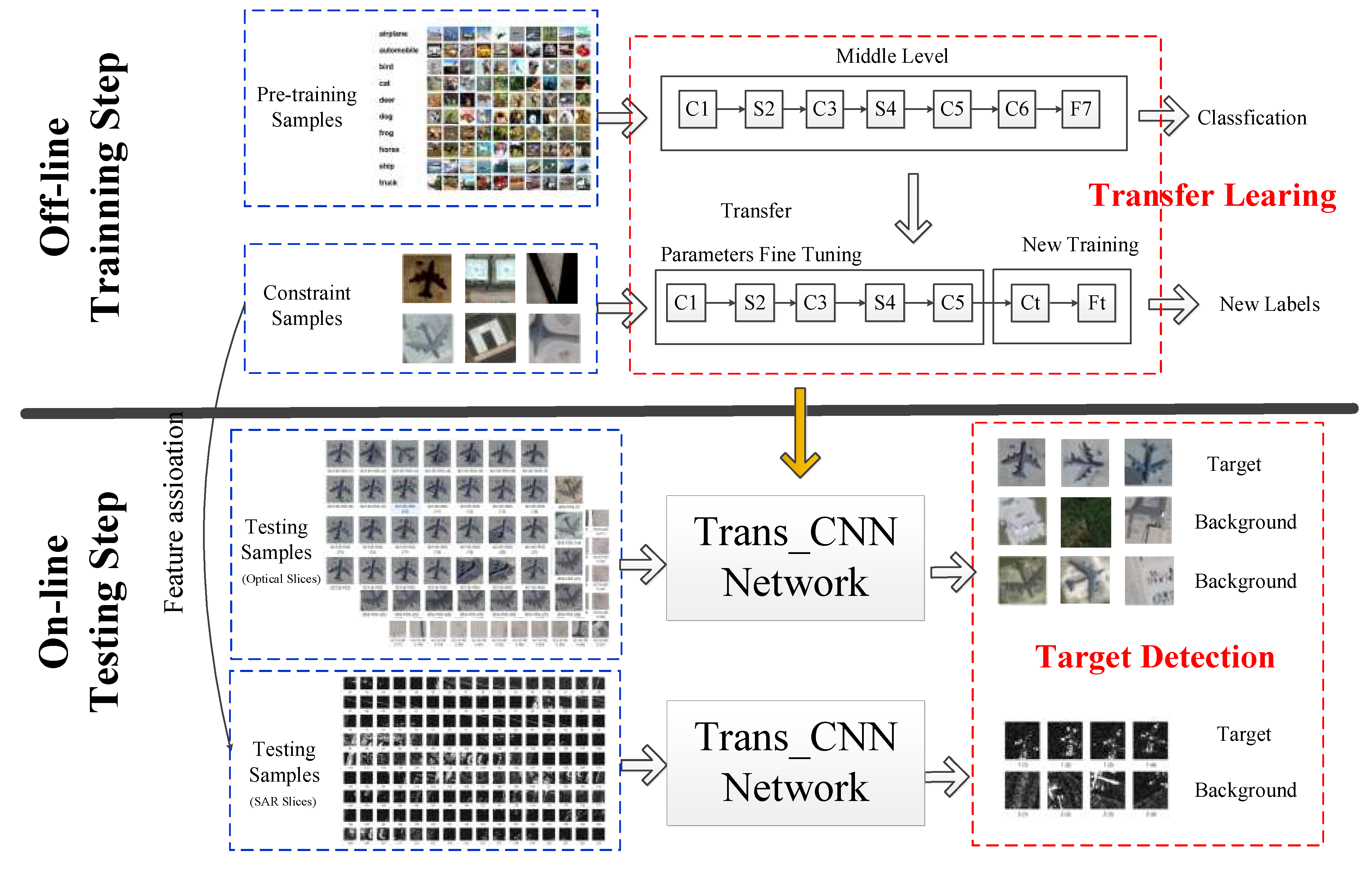
The flowchart of the proposed method is presented in Figure 1. The two main phases are the off-line training step to build a stable network driven by specific targets and the online testing step to complete the detection task. A two-step training method is adopted in the training step. Firstly, a B_CNN network is trained using a CIFAR-10 (see details in Section 3.1) dataset to develop a stable model. This B_CNN shows a great potential to extract general shape features. It also appears sufficiently flexible to abstract similar features from different domain slices. It is the base to undertake the fast switching of target detection tasks.
Secondly, a Trans_CNN is retrained on small number of constraint samples to highlight the target characteristics in the specific detection task. It has a nearly identical convolution and pooling structure as B_CNN, although its convolution layer and full-connection layer are new (see details in Section 2.3.1). In this step, a FA is necessary to improve the performance of knowledge transfer in Trans_CNN if the constraint and testing samples stem from SAR and optical sources.
The two-step training method is not an unrolled version of traditional training methods in CNN. It is, instead, a state-of-the-art method focused on the question of small numbers of training samples.
At first, FA can be used to extend training samples with relatively easy to acquire optical images for SAR target detection. It can unify the optical and SAR images at feature levels to enriching the features in the target domain. However, in many cases, as one of the real remote sensing images, the number of optical images of such targets is still insufficient to support the training of CNN. Therefore, B_CNN pretraining is performed with the sample-rich CIFAR-10 database. Because of the local receptive field in the CNN, the network is concerned with local simple structures within the view field but not the entire input images. These structures such as corners, small circles, or sharp angles are the basis for any input; they are the general features in any type of image. The role of CIFAR-10 is to grant the B_CNN the ability to recognize these general features.
In this paper, the pretraining of B_CNN is not performed using remote sensing data as the CIFAR-10 contains more categories and more comprehensive types of general features. Meanwhile, as camera images, the general features of the images inside are clearer and easier to learn. Therefore, the resulting B_CNN is more sensitive to structural details and can flexibly achieve target switching in different tasks. It effectively increases the generalisation ability of the network. In addition, unlike classification tasks, each category is a clear arrangement and combination of general features. In target detection tasks, ground objects contained in background categories are complex. Usually, no uniform distribution can fully cover them, as this also requires B_CNN to have sufficient knowledge of the various general features.
Then, a well-directed constraint training is performed to enhance the network’s perception of the target characteristics. Fine-tuned parameters can be focused on the target category, while the labels of the new task are defined in a new, fully-connected layer. In this way, a limited prior knowledge can be maximised.
With the help of data fusion, this two-step training method gradually solves the issue of non-homogeneous prior samples in the target domain. Namely, the sample-free situation in the target domain is first improved to a heterogeneous small sample situation. Finally, the training of the network is completed using a powerful standard data set. The number of constraint samples is too small compared to any type in CIFAR-10 to mix all the samples together. Indeed, mixing them together would cause a sample imbalance problem, thus easily overwhelming target features. Moreover, the two-step training method can achieve rapid task switching and differs from other methods in preventing this problem by optimising the network structure. For different targets, only the corresponding constraint samples need to be selected in constraint training. It is not necessary to retrain B_CNN. The generalisation ability of the network can thus be greatly improved.
2.2. Feature Extraction and Transfer Learning in CNN
2.2.1. Feature Extraction in B_CNN
The convolution neural network (CNN) alternately uses convolution and pooling layers to extract the features of the inputs. The extracted features, named mid-level representations, are higher-level features which are more abstract than simple low-level features.
In the hidden layer, the previous layers’ input feature maps connect to all the output feature maps. Each unit in the convolution, pooling and full-connection layers, are computed as Equations (1)–(3). Besides, is the feature map of layer in the hidden layers. is the weight matrix representing the convolution kernel (trainable filter). serves a bias term. is a non-linear activation function and subscript represents the full-connection layer.
Similarly to most machine learning algorithms, all weights and biases are learned via minimising a loss function (see Equation (4)). It is usually impossible to analytically compute the global minimum of the loss function. Minimising the loss function through an iterative numerical optimisation approach is therefore a widely accepted method. The gradient descent is the simplest of such optimisation algorithm.
Then, a BP (Back Propagation) algorithm is adopted to iteratively update the parameters. The error term of layer is calculated in Equation (5), where is the transposition of the weight matrix for the layer [43]. e denotes the element-wise product of the two vectors.
In the convolution or pooling layer, the error term can be rewritten as Formula (6) or (7). rot180() represents the symmetric exchange in the row and column, respectively. upsample() is the function used to complete the error matrix amplification and error redistribution. The reduction size depends on the pooling layer. The parameters in iteration refreshed as Equation (8). is the learning rate.
2.2.2. Transfer Learning of Trans_CNN
The knowledge-transfer approaches assume that the individual models for the related tasks should share some parameters or prior distributions of hyper-parameters. They aim to boost the performance of the target domain by using the source domain data. The proposed method assumes that in CNN, the parameters W for each task can be separated into two terms [26]. One is a common term over tasks while the other is a task-specific term (see Equation (9)). and are the parameters of CNN for the source and the target tasks, respectively. represents the common ones that can be transferred. and are the specific settings for the source and target domain which need retraining separately. In this paper, source tasks denote the classification tasks trained by the picture of computer vision, while the target tasks refer to the detection tasks driven by real remote sensing images.
Taking the convolution layer in the source domain in feed-forward pathway as an example (see Equation (10)), the following equation will be used based on the operational mathematical properties of the convolution:
Then, the assumption (Equation (9)) is applied to the feed-forward pathway (Equations (1)–(3)) and back-propagation phase based on the Formulas (6) and (7). In both the source and target domains, the final expression can be rewritten as shown in (Equations (11)–(14)). Besides, , , represent convolution, pooling and full-connection layers, respectively.
The feed-forward and back-propagation phases (Equations (11)–(14)) in both source and target domain tasks can be divided into two independent parts. This means that the parameters in the CNN can be trained separately in multiple steps and by different samples. The common ones related to can be transferred directly. And the target part connected to needs to be calculated by task-specific constraint samples. The source part tied to should be abandoned. The nonlinear function in the and layers can be similar or different. This derivation serves as the theoretical basis for the learning algorithm used in this paper.
2.3. Network Structure and Learning Algorithm
2.3.1. The Structure of B_CNN and Trans_CNN
B_CNN and Trans_CNN depict structures similar to LeNet-5 [44] which is considered as the most basic and original version of CNN. Their nine layers are presented in Figure 2. Besides, C, S, and F represent the convolution, pooling, and full-connection layers, respectively. fm represents the feature maps in each hidden layer. Size represents the size of input maps in each neuron. In the convolution layers, the number of feature maps and filter sizes is marked on the left and right sides of @. The pooling parameter set in this paper is the commonly used 2 × 2 with a stride of 2. The feature vector is a concatenation of all the feature maps in C6 or Ct. It is a visual expression of the differences between target and background.
A sigmoid function is applied to each unit as the nonlinear activation function during the entire training process. The outputs in F7 (Ft) are the label distributions of each input slice. In the testing step, these values indicate the confidence in the classification of testing slice to one type. The label distributions of a well-trained network should meet the following requirements. Firstly, the probability of the right label should be much greater than others, so that the classifier can resolutely decide that the input belongs to the correct type. Secondly, for a set of the input slices belonging to the same type, the peak of the possibility distributions must overlap on the suitable label to demonstrate the robustness of the network. Intermediate schematics are presented at the bottom of Figure 2. Part of the feature maps are displayed from left to right in hidden layers, feature vector in C6/Ct and label distribution in F7/Ft, respectively.
2.3.2. Training Algorithms in B_CNN and Trans_CNN
The training step can be divided into two phases. One is the B_CNN pretraining, while the other is the Trans_CNN constraint training driven by specific-tasks. The training method used in each phase is the same as the usual training method employed in CNN [44].
Firstly, the C1-C6 and F7 of the B_CNN are trained on the CIFAR-10 dataset. Then, the last convolution layers C6 and layer F7 of the B_CNN are removed, while the rest of the C1-C5 layers act as a mid-level representation extractor transferred to the target domain with fixed parameters. To accomplish transfer learning, an adaptation network is added which includes a new convolution layer and a new full-connection layer named Ct and Ft. In the full-connection layer, Ft is calculated by Equation (15), where is the production of the new convolution output. and are the parameters that need to be trained. is the non-linear activation function.
Secondly, the representation is available to train the entire network formed by C1-Ft layers. The previous convolution and pooling layers are imitated from the B_CNN, and with revisions of the parameters based on the constraint samples. The Ct output is the final representation of the target in SAR images. After completing constraint training, the transformed layers C1-C6 and the adaptive layers Ct-Ft can form the Trans_CNN together to detect target in target domain. The training algorithm is shown in Table 1.
2.4. Feature Association in SAR and Optical Samples
2.4.1. The Feature Association Model
The harmonization of the SAR and optical images in feature levels is majorly covered in the research paper on registration. For example, a novel structural descriptor, the PCSD (phase congruency structural descriptor), is constructed to accurately describe the attributes of extracted points [45]. For this purpose, descriptor similarity and geometrical relationship are combined to constrain the matching process in order to significantly increase the number of correct matches [46]. The coupled optical and SAR patches for different sources are then automatically extracted by the learning features in the pretrained network Pseudo-Siamese CNN [47] and generative matching network (GMN) [48], respectively. At the same time, in [49], the corresponding SAR-like images are constructed via conditional generative adversarial networks (cGANs). In this regard, improving the accuracy of ground control points selection proves to be effective.
Constraint training in this research aims to transform the B_CNN network from a focus on the general features to the target features to be detected. Therefore, it is necessary to approximate the characteristics of the specific target from multiple sensors as closely as possible to the test sample in the constraint training.
According to the operational flow, from the actual existence of ground objects to feature vectors for category determination, this training can be generalised into three steps. As shown in Figure 3, imaging processing, image information acquisition, and feature space projection are respectively performed. Because of the difference in imaging mechanism, optical and SAR images have large differences in the form of target existence and data processing. However, because the objects to be imaged are the same, there must be overlapping parts in a certain feature space. Therefore, this intersection is where the FA are concerned.
According to Figure 3, the optical and SAR imaging process can be expressed as Equation (16). Besides, represents the true three-dimensional information of the target. and represent different imaging functions. and are optical and SAR image amplitudes.
In the information acquisition process (step 2, see Equation (17)), and are the image effective information acquisition function. It is a generalized operation including pre-processing such as denoising filtering, data-level operations such as image rotation and stretching and transformation, and even feature-level operations such as feature extraction and component analysis. Any set of operations can be included in this function for the purpose of subsequent processing of the required information acquisition. and are the effective source and target domain information obtained after the operation. Because of the obvious difference of the acquisition path, in the case of this expression, there may or may not exist intersection information.
In step 3, the effective feature space projection method is used to make the source domain feature and the target domain feature intersection as large as possible in the new feature space. This process is shown in Equation (18). Besides, and are a set of functions related to features in source and target domains respectively. and are the source and target domain feature in the new feature space. As shown in Figure 3, . In both domains, subscript i denotes the identical features, while d denotes the different ones.
According to the mathematical definition of the intersection . The intersection of the feature can be written as Equation (19).
In both source and target domains as Equation (20), and are the intersection obtained by calculation. and are the functions to extraction the overlapping parts.
Compared with the real ones in Equation (19), . and are the extraction errors. In the new feature space, let . So far, the unit domain and the target domain are unified at the feature space level. The relationship of the entire feature space can be expressed as Equation (21).
In this way, by continuously taking the inverse operation, it is possible to complement information across the disjointed parts of the source in any intermediate process. This is a mathematical model of feature association. In practical applications, the complexity of each operation function is different, and the feasibility of the inverse operation is also uncertain. It is determined by the actual situation.
2.4.2. Association Algorithms
In high-resolution SAR images, a large-size target is composed of several pixels. Instead of a single bright spot, it appears as bright regions marked by dim and dark. It is a common occurrence that the target body contains holes inside and fractures on the edge. Even the frames extracted from SAR images are not continuous. Even though CNN can extract the abstract features implied in the structures, the presentation difference between optical and SAR images could not be neglected.
The key is to construct a new feature space where the extracted features from multiple sources are similar. In the absence of any prior samples of SAR slices, the straightforward starting point is the deformation of appearance in multiple sources. Therefore, FA in this paper is more likely a pre-processing. In this processing, the optical slices are deformed to simulate SAR slices. The different steps for constraint training and testing samples are presented in Table 2.
The threshold segmentation is an effective way to highlight the consistency of target appearance and to avoid the influence of grey differences in multiple sources. For SAR, frost filtering is adopted to reduce speckle noise. Framework extraction is another way to evade the incompleteness of target body in SAR images. Frameworks randomly rupture human-made intervention to imitate the fracture in the SAR framework. Finally, mathematical morphology includes three common operations for both samples and a special one for SAR slices. Operation ‘skel’ can further refine the framework. Operation ‘bridge’ can connect the proximity points. Operation ‘dilate’ can plump the frame to restore the target and background. It is useful to widen the differences in shape features between the target and background.
This method does not seem complicated, but it is effective without the need for SAR source prior samples.
3. Results
3.1. Experiment Data and Evaluation Metrics
The CIFAR-10 dataset is commonly used in image classification research. It consists of 10 classes of colour images with a size of 32 × 32, containing a total of 60,000 copies. Each type includes 6000 slices distributed in five batches. The ten types are airplane, automobile, bird, cat, deer, dog, frog, horse, ship, and truck. These images are captured in camera perspective which is absolutely different from the remote sensing images. In this paper, the main purpose of this dataset is to pretrain the B_CNN.
The target slices are cut from real remote sensing images in multiple satellites. The specific target in this paper is a KC135 airplane, and the target is located at the Al Udeid Air Base, Qatar. The target and background slices in different sensors are presented in Figure 4. Besides, Figure 4a includes optical slices with 0.5 m resolution in Google earth named optical A The set contains 255 couples of positive and negative samples in time sequences. Meanwhile, a B52 airplane serves as the similar interference, a total of 200 slices captured from another scene are prepared in this set. Figure 4b includes optical slices from Quickbird satellites, named optical set B. A total of 36 slices are sourced from only one image. Figure 4c is SAR slices in Terra_SAR images with 1 m resolution. The whole image contains 27 KC135 airplanes. Therefore, the testing samples include 27 positive and negative samples, respectively. It can be seen clearly that the same objectives in multiple sensors share a similar structure even though they are presented quite differently.
The evaluation metrics in this paper are defined in Equations (22)–(25). The accuracy (), and the detection rates of target and background ( and ) are used to evaluate performance in a binary classification task (e.g., in Section 3.2). Meanwhile the criteria focused on the target is more crucial in the target detection task (e.g., in Section 3.3). Thus the evaluation metrics are accuracy (), precision (), and false-alarm rate (). N denotes the number of true positives (TP), true negatives (TN), false positives (FP), and false negatives (FN). In this paper, images with a KC135 are defined as positives; while images without KC135 are negatives.
C is the correlation coefficient to analyse the correlation relationship between the feature vectors of slice couples in FA results (e.g., in Section 3.3.2). It is not a classic means for target detection. In this paper, it is used in the section for feature association part to measure similarity between feature vectors of two input slices. As the FA algorithm proposed in this paper tends to increase the similarity between target slices taken from different sources as well as the difference between two types (target and background).
The experiments in this paper are set as follows. Section 3.2 discusses the structure and training method. It proves that Trans_CNN is suitable for the target-driven detection task. Section 3.3 shows the detection results for real remote sensing images. With the help of FA, the Trans_CNN out performance in both the multiple sensors from optical and multiple sources.
3.2. Trans_CNN Structure and Training Method
3.2.1. Trans_CNN Structure
Figure 5 is the label distribution of the different target or background slices. It indicates the confidence of the testing slices to be classified into one type. The first row denotes the target, and the second represents the background. The number of input slices is 10, and their responding output label distributions are presented in one figure with different colours. One colour line represents one input.
The KC135 airplane from optical set A is a new type for B_CNN whose feature is different from all the types in CIFAR-10. Even though the B_CNN is strong enough to extract the mid-level features from input slices, it is puzzled by their labels. Therefore, in Figure 5a,d, the peak of the label distributions is confusing in B_CNN for both target and background. It means that, for the same input slices, B_CNN classifies them into different types. In each classification process, the confidence is less than 60%. Taking the red curve in Figure 5a as an example, for this input, B_CNN classifies it into type 3 with a probability of 0.45, type 6 with 0.4, and the other types with smaller expectations. At this time, constraint training is essential to let the network know the features and their labels in the new task. It can be seen from Figure 5b,e that the confusing output is consistent by parameters fine-tuning. The network has a new unified understanding of the features in the target domain. For the target detection task, there are only two types, namely target and background. Other types are useless. Therefore, in the constraint training step, a new connection between the constraint training samples and new task labels in the target domain is rebuilt. This connection is independent of the full-connection layer in B_CNN. Therefore, in Figure 5c,f, there are only two types. Label 1 belongs to target, and label 2 belongs to background.
The probabilities of the input be classified to one type are recorded in Table 3. It is a quantitative representation of Figure 5. It can be seen from the comparison that the method proposed in this paper can achieve high output confidence for the specified tasks.
Figure 6 illustrates feature vectors extracted from different networks trained using various samples. It is a visual expression of the differences between target and background. The inputs are the slices of the target (the first row) and background (the second row) from the SAR image. Network A refers to B_CNN trained on CIFAR-10 only, however in network B (Trans_CNN), 5 couples of real remote sensing samples are added to constraint training. Moreover, Network C denotes a CNN network with the same structure, but it is trained on samples in optical set A only. It contains maximum amount of information that can be obtained for a target. The differences between target and background are more evident in Trans_CNN than in the others. This is the original reason to detect the target in SAR images by Trans_CNN only trained on the constraint of optical samples. Even though the features are different in the two domains, there are many more divergences between target and background.
3.2.2. Discussion of Training Method
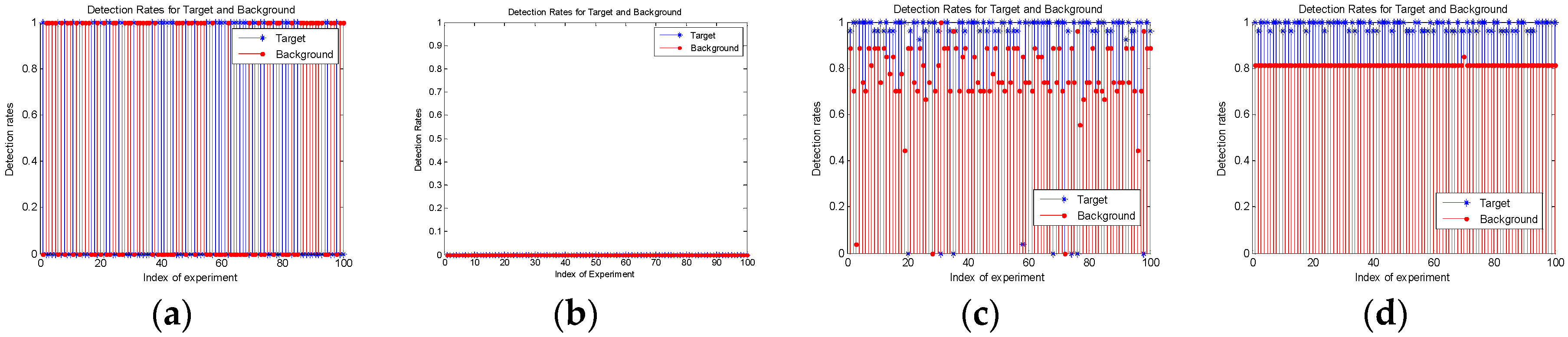
Different training methods in this part are shown in Table 4. Besides, ‘SAR’ represents the original SAR slices selected from testing samples. The number of positive and negative samples is 5 respectively, which equals to the ones in constraint training. In these training methods, ‘together’ means the positive and negative samples to be tested are mixed into CIFAR-10 as separate categories (type 11 and 12 respectively), and training is performed simultaneously with all samples. The ‘apart’ is the pretraining plus constraint training method proposed in this paper. For (a) and (b), the training step is identical to the traditional CNN. But for (c) and (d), multiple training means the constraint training step in Trans_CNN.
Figure 7 is the compared results of the above training samples in the off-line training stage. The training and testing are conducted 100 times to verify the effectiveness and robustness of the networks. The mean values of these 100 detection rates are recorded in Table 5. All 1s and 0s in Figure 7a verify that the network failed to distinguish the target and background in each train and test when prior samples are limited. In Figure 7b, no matter the target or background, they were unable to distinguish them all 100 times. That is because the number of their training samples is too small compared with the other types in CIFAR-10. It is inferior for these samples to affect the parameters in the CNN. The sample imbalance in this training phase causes the fact that although data is enough to train the network, it is very insensitive to the task-driven targets and background slices that really matter. Effective prior samples are overwhelmed. Even though Figure 7c can achieve a 0.9 detection rate in mean value, there still some zero points, which means that the network failed to find the target in this training. In real applications, this failure is fatal even though it seldom appears. The phenomenon does not appear in Figure 7d, and the curve is very steady, proving that the network is stable. The proposed method is not only out-performing in the detection rates but also in stability. This is because the network learns the general features in the pretraining phase, independent of the specific goals. Generally, the more diverse the training samples, the more flexible a network will be.
Comparing Figure 7a,c,d, it is stated that the small sample problem can be solved by the pretraining method. The richer pretraining sample categories, the more stable the network. Comparing Figure 7b,d, the two-step training method can solve the sample imbalance problem. The same training samples can achieve different result through different training methods. In a word, the two-step training method proposed in this paper can maximise the valuable limited priori knowledge.
3.3. Target Detection in Heterogeneous Sources
3.3.1. Transfer Learning in One Source from Multiple Sensors
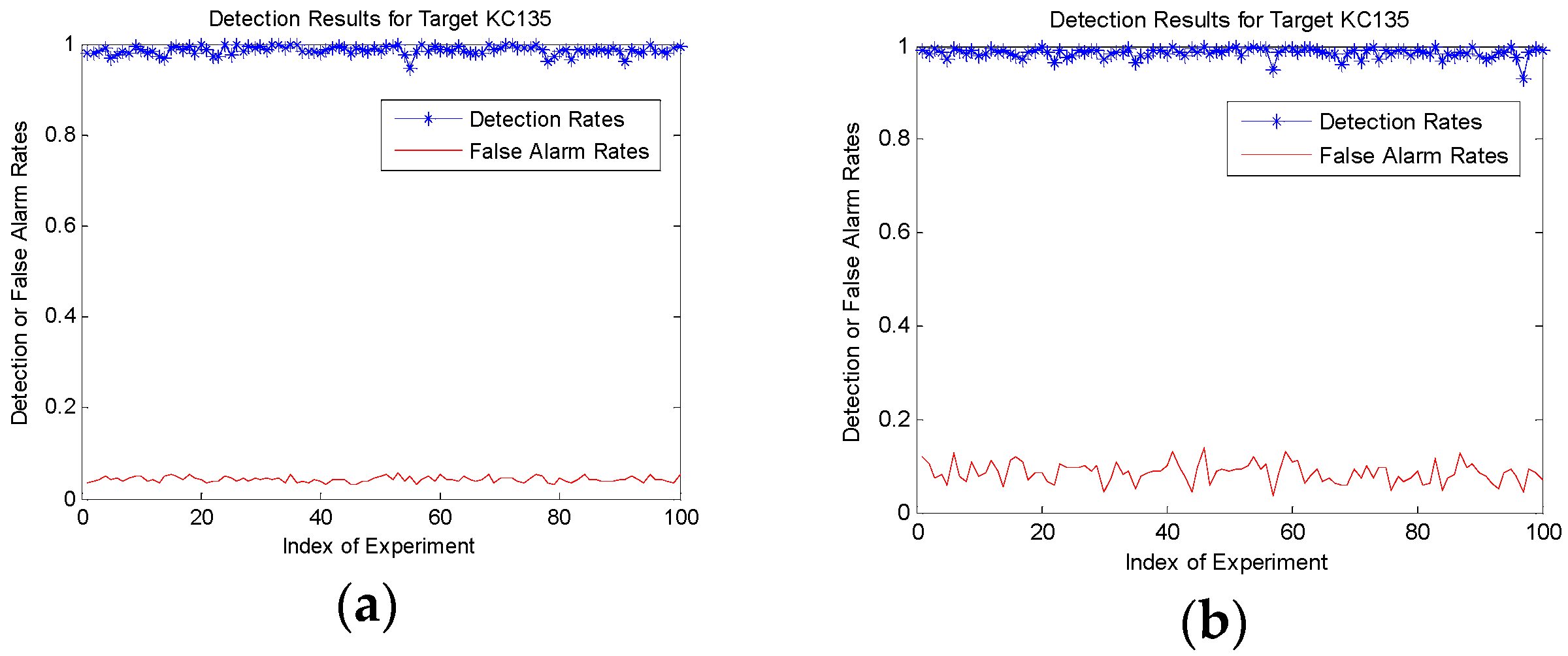
In this section, the constraint and testing samples stem from optical sets B and A, respectively. Figure 8 is the 100-time detection results containing the detection and false alarm rates. Besides, in experiment (a), the target and background slices are getting from one screen in time sequence containing only KC135 plane as target and the other objectives as background. There is no other type of aircraft involved in the background slices. In experiment (b), a B52 airplane acting as a similar interference is added to the background slices. A total of 200 slices mixed with B52 aircraft and other objectives are captured from another screen with 0.5 m resolution in Google earth. It is used to verify the Trans_ CNN ‘s ability to distinguish the target and its similar type of interference.
Table 6 shows the quantitative results. Columns 1–5 represent the records of the first five times. Max and min mean the best and the worse performance according to the detection rates. Mean is the mean value of all these 100 times. Results demonstrate that the Trans_CNN is competent for this target detection task where homologous prior samples in the same sensors are unavailable. Even if there is a similar interference of the same type in the background, test results only show a measurable increase in the false alarm rates.
3.3.2. FA Results
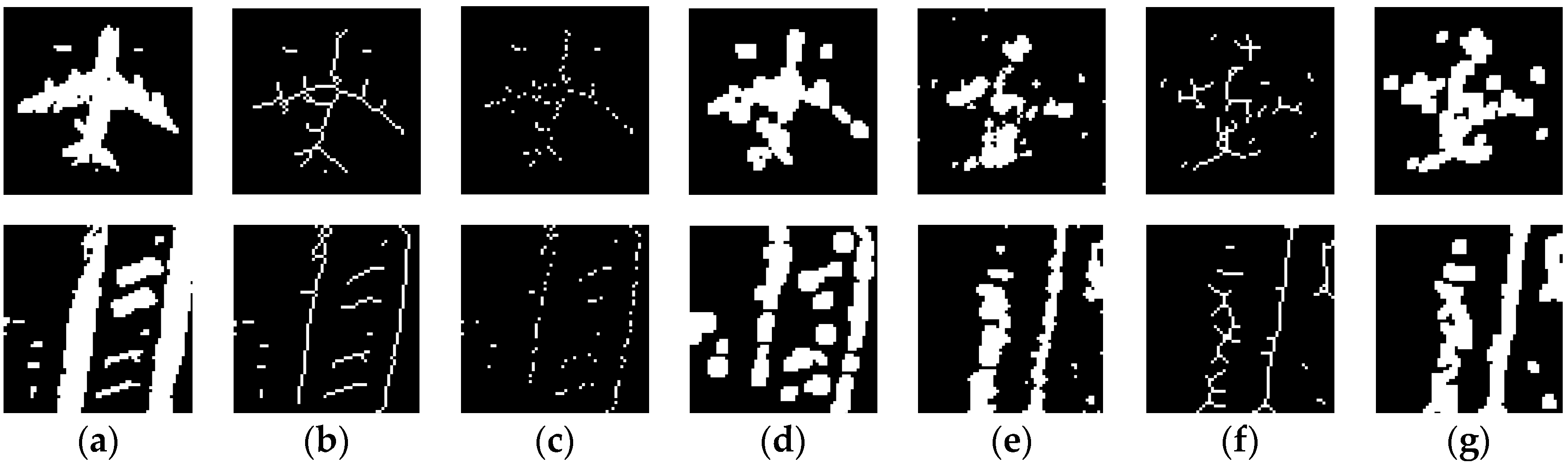
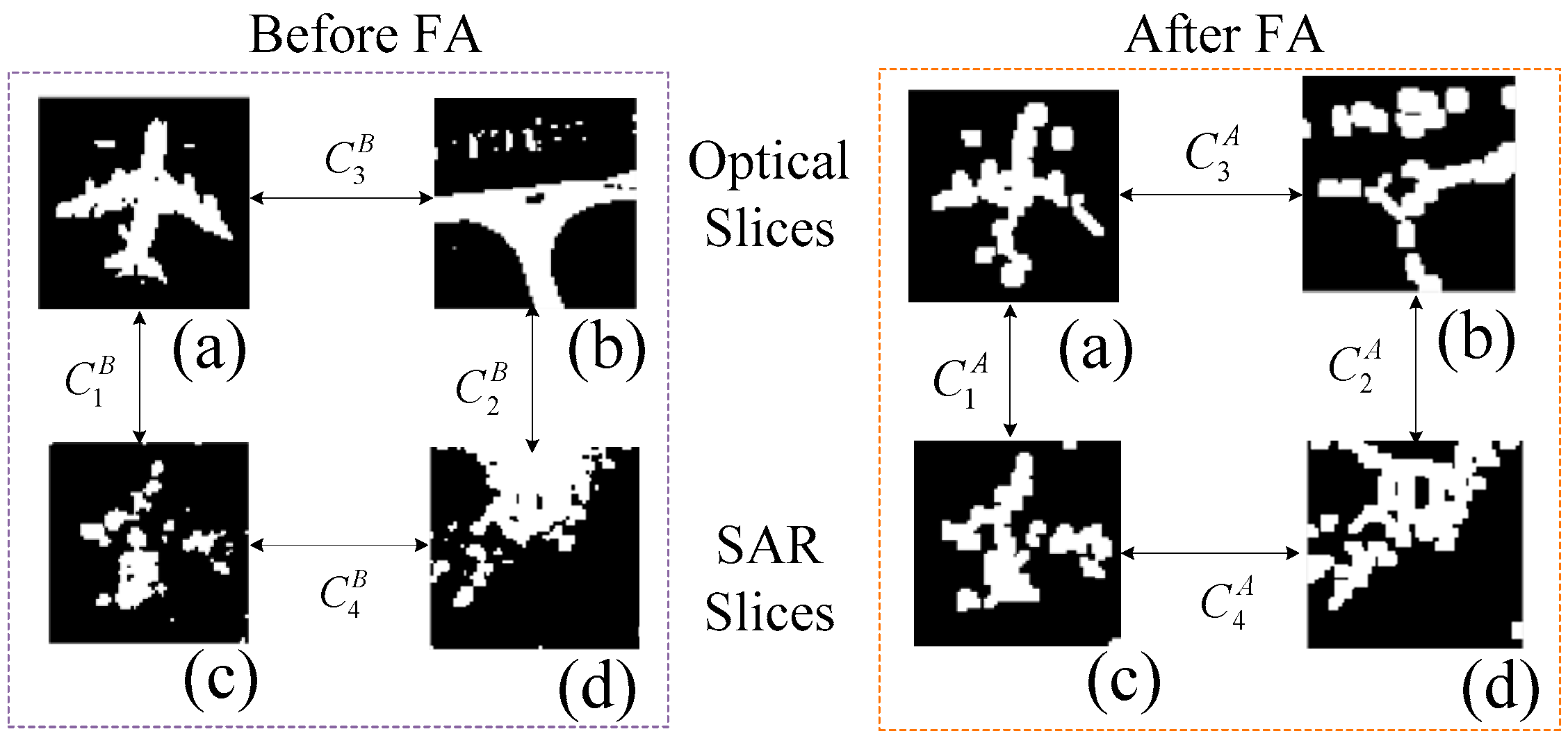
In this section, the constraint and testing samples stem from optical sets A and SAR, respectively. Figure 9 is a visual display of FA results of the target and background slices. The background slices in two sources are not entirely corresponding (Figure 9a,e). From Figure 9d,g, the samples in different sources have a similar presented form. Compared with Figure 9a,e, it is more relevant as the training and testing samples.
In order to better explain the effect of association, the concept of correlation coefficient is introduced to analyse the correlation between any two groups of slices. The slices and correlation coefficient in corresponding positions are shown in Figure 10.
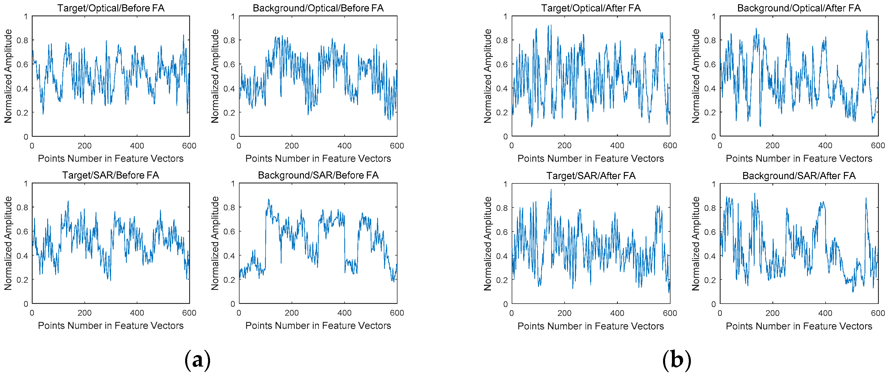
The feature vectors of these slices are shown in Figure 11. It intuitively shows the increasing similarity of the target.
Part of the couple correlation coefficients are recorded in Table 7. Besides, the first column is the number index of target and background couples in the optical set A and SAR dataset. Corresponding to Figure 10, target couples contain slices similar to Figure 10a,c while background couples to Figure 10b,d. The desired result are as follows. Firstly, C1 and C2 become larger. It represents the increasing similarity between the similar objectives. Secondly, C3 increases. The similarity increases of the label are equivalent to making the network more sensitive to the differences between target and background. Thirdly, C4 becomes smaller. A decrease in correlation means an increase in the distance between the types. It contributes to distinguish target from background.
It can be seen from Table 6 that the change trend of C1, C3, and C4 are in accordance with the desired results. But C2 is not. For the detection task, the target is more important than the background. It is acceptable to obtain higher target similarity at the expense of background similarity.
3.3.3. Transfer Learning in Multiple Sources
The 20 times detection results that depend on different feature spaces are shown in Figure 12. In the separate feature space, the constraint training and testing samples are processed in a different method. The mean detection and false alarm rates are presented in Table 8. Time means the time cost of one constraint training and testing session.
Regarding the FA performance, we need to describe the following three aspects.
1. For target detection tasks, accurately determining the existence of the target is far more critical than any other evaluation index. The method proposed in this paper has apparent advantages in detection rates.
2. The time consumption in FA slightly increases compared with Figure 12a,c. Their constraint training samples are the small part of the total in common. But in contrast with Figure 12b,d with all slices in constraint training, the proposed method can save a lot of training time significantly. What needs emphasising is that, in all the above detection tasks, the B_CNN is the same one trained only once. The Trans_CNN is trained on the constraint samples based on the mission to fine-tune the parameters in B_CNN as well as the new convolution and full-connected layers. This constraint training can be finished in quite a short time. Thus, the network proposed in this paper significantly reduces the switching time between detection tasks and improves the generalisation ability of CNN.
3. At last, in this part, there is no contrast between the proposed method and the other machine learning methods about the detection rates; for the main point of this paper is to solve the problem with which the traditional CNN was unable to deal, namely, a detection task without homogeneous prior samples. Under the implementation conditions of each experiment in this paper, traditional CNN cannot complete the test at all.
4. Discussion
4.1. The Performance of CNN
The starting point of this paper is a novel application of CNN in real remote sensing images to solve the problem of the limited quantity of prior samples. It is very common in actual remote sensing applications, just as the experiment in Section 3.3, that the homogeneous training samples are unavailable. Even the same type of target in the optical source is in limited quantity. Therefore, the proposed method is an innovative solution to the actual problem, rather than structural adjustments on the original CNN framework, to achieve performance improvement. The detailed adjustment is important to increase performance. But the feasibility of the system is the basis and premise of all improvements.
The network in this paper is the basic one proposed in [44]. The following improved algorithms of the CNN are also suitable for the B_CNN and Trans_CNN in this paper, such as the “dropout” to improve the overfitting, the replacement of sigmoid to “ReLU” in nonlinear functions, the usage of “softmax”, and so on.
The final detection results are related to the training of B_CNN and Trans_CNN. In every constraint training, the feature vectors are decided by the network parameters. Therefore, the results have a certain randomness. The same curves in Figure 8 and Figure 12 are difficult to reproduce. But the comparison results and mean values presented in Table 5 and Table 7 are almost the same.
The constraint training and testing was conducted several times for two reasons. Firstly, a stable and robust network can get a steady detection rate in each experiment. Secondly, the mean performance is much closer to the real ability of the network.
4.2. The Explain of Comparison Results
The CNN can get a good prediction of the testing slices based on the statistics derived from a large number of training samples in each label. Most of the deep machine learning algorithms in SAR images is conducted on MSTAR (Moving and Stationary Target Acquisition and Recognition) datasets. The publicly released data sets include ten different categories of ground targets from armoured personnel carrier, tank, rocket launcher, air defence unit, truck, and bulldozer. The objectives in different aspect angles and depression angles are also included. The MSTAR benchmark data set is widely used to test and compare the performances of SAR-ATR (Synthetic Aperture Radar Automatic Target Recognition) algorithms.
But in the real application, the recurrence of such a sample-sufficient training data set is impractical. The proposed method pays attention to the detection task in the absence of prior samples. Under this condition, the traditional CNN cannot be trained. The preconditions are far from each other, so the comparison is far-fetched and meaningless. Hence, in other machine learning models, such as SVM (Support Vector Machine), ANN (Artificial Neural Network), ELM (Extreme Learning Machine), or AdaBoost numbers of labelled prior samples are required throughout the training steps.
The same rational is applicable to the algorithms related to transfer learning. They focus on supervised classification task. The homogeneous samples are more or less available. The unbalanced number of samples is an essential difference between target detection and classification tasks. Meanwhile, classification tasks work well with common characteristics of the same category. On the other hand, target detection tasks, although considered as a two-category classification system, majorly encompass the specific characteristics of a target. Therefore, with the non-homogeneous samples used in this research, the network training used and transfer learning applications are both different from those used in traditional conditions. The method proposed in this paper is based on real remote sensing images and focuses on specific target-detection applications. The experiment demonstrated that detection can be completed without homogeneous training samples.
4.3. Discussion of High False Alarms
Figure 13 shows the relationship between the number of constraint samples and detection rates. The samples in optical set A are sufficient to carry out this experiment. Therefore, in this experiment, the pretrain data set is CIFAR-10, and the constraint training samples are a different number of couples selected from optical set A. The testing samples include all the slices in optical set A. It can be seen that, as the number increases, the detection rates increase slightly both in target and background. Due to the various objectives in the background, even though the training and testing samples are from the same sensors, the high detection rate of the background (i.e., low false alarm rate) is challenging. When the number is 5, given the same condition as Section 3.3.3, the false alarm rate is 0.19.
Therefore, in Figure 12a,c,e, the limited number of prior samples in constraint training will inevitably introduce higher false alarms. Because unlike a specific type of target in only one species, the background slice contains a variety of substances, such as roads, soil, man-made buildings, and other analogous-target objectives. The training samples can hardly cover the general distribution of all these terrains. This phenomenon can be demonstrated in Figure 13. Meanwhile, the imaging presentations of heterogeneous data and the large interception during the slicing process are other reasons for the differences.
4.4. Future Studies
Feature association is an effective way to regulate the differences between the source and target domains. The method proposed in this paper is more likely a pre-processing focused on the presentation in different sources. This is a compensation method under finite conditions of SAR prior samples. In future studies, association algorithms related to the target characteristics or the feature with the physical property are meaningful.
The target detection task can be seen as a classification of one against the others. The false alarms are equivalent to the right background classification. When dealing with the problem of the small quantity of training samples, how to take advantage of the limited information of prior terrain samples to cover the complex feature of background slices is also an issue to be studied.
As previously mentioned in the abstract, the initial starting point of this research was to explore a state-of-the-art method for overcoming inadequate sample problems in real remote sensing applications rather than produce a preliminary version of training methods or promote structure improvement in CNN. Thus, this paper comprises discussions about methods used to complete detection tasks when the usual CNN fails to work. It is noted that more indicators are needed to enrich the evaluation system to devise a perfect detection method, which shall be covered in subsequent studies.
5. Conclusions
In this paper, a target detection method based on knowledge transfer and feature association was developed for remote sensing applications. The scarce feature in target domain caused by the lack of prior samples in SAR source was expanded through feature association from heterogeneous samples in optical sources. Moreover, these features could be effectively extracted by the Trans_CNN with knowledge transfers from a basic CNN once trained by a comprehensive data set in the future. Finally, a higher than 0.85 detection rate could be achieved in the real image experiment. The problem of invalid models in traditional CNN without homogeneous prior samples was solved through a step-by-step process.
Author Contributions
For research articles with several authors, a short paragraph specifying their individual contributions must be provided. The following statements should be used “conceptualization, G.Z. and Y.Z.; methodology, G.Z.; software, G.Z.; validation, G.Z., Y.Z.; formal analysis, G.Z.; investigation, G.Z.; resources, Y.Z.; data curation, G.Z.; writing—original draft preparation, G.Z.; writing—review and editing, G.Z.; visualization, G.Z.; supervision, Y.Z.; project administration, Y.Z.; funding acquisition, Y.Z.”, please turn to the CRediT taxonomy for the term explanation. Authorship must be limited to those who have contributed substantially to the work reported.
Funding
This research was funded by the Defense Industrial Technology Development Program, grant number JCKY2016603C004.
Acknowledgments
The authors would like to thank Professor Junping Zhang, Hao Chen and Xinyuan Miao, Shoulin Yin, Wen Chen for their help to finish this paper.
Conflicts of Interest
The authors declare no conflicts of interest.
References
- Haitao, L.; Siwen, W.; Yongjie, X. Ship Classification in SAR Images Improved by AIS Knowledge Transfer. IEEE Geosci. Remote Sens. Lett. 2018, 15, 439–443. [Google Scholar]
- He, C.; Xiong, D.; Zhang, Q.; Liao, M. Parallel Connected Generative Adversarial Network with Quadratic Operation for SAR Image Generation and Application for Classification. Sensors 2019, 19, 871. [Google Scholar] [CrossRef] [PubMed]
- Eldhuset, K. An automatic ship and ship wake detection system for spaceborne SAR images in coastal regions. IEEE Trans. Geosci. Remote Sens. 1996, 34, 1010–1019. [Google Scholar] [CrossRef]
- Lombardo, P.; Sciotti, M. Segmentation-based technique for ship detection in SAR images. IEEE Proc.-Radar Sonar Navig. 2001, 148, 147–159. [Google Scholar] [CrossRef]
- Smith, M.E.; Varshney, P.K. Intelligent CFAR processor based on data variability. IEEE Trans. Aerosp. Electron. Syst. 2000, 36, 837–847. [Google Scholar] [CrossRef]
- Blake, S. OS-CFAR theory for multiple targets and nonuniform clutter. IEEE Trans. Aerosp. Electron. Syst. 1988, 24, 785–790. [Google Scholar] [CrossRef]
- Kefeng, J.; Xiangwei, X.; Huanxin, Z.; Jixiang, S. A Novel Variable Index and Excision CFAR Based Ship Detection Method on SAR Imagery. J. Sens. 2015, 2015, 437083. [Google Scholar]
- Yu, W.; Wang, Y.; Liu, H.; He, J. Superpixel-Based CFAR Target Detection for High-Resolution SAR Images. IEEE Geosci. Remote Sens. Lett. 2016, 13, 730–734. [Google Scholar] [CrossRef]
- Wang, C.; Bi, F.; Zhang, W.; Chen, L.J. An Intensity-Space Domain CFAR Method for Ship Detection in HR SAR Images. IEEE Geosci. Remote Sens. Lett. 2017, 14, 529–533. [Google Scholar] [CrossRef]
- Wang, S.; Wang, M.; Yang, S.; Jiao, L. New Hierarchical Saliency Filtering for Fast Ship Detection in High-Resolution SAR Images. IEEE Trans. Geosci. Remote Sens. 2016, 55, 351–362. [Google Scholar] [CrossRef]
- Bi, F.; Zhu, B.; Gao, L.; Bian, M. A visual search inspired computational model for ship detection in optical satellite images. IEEE Geosci. Remote Sens. Lett. 2012, 9, 749–753. [Google Scholar]
- Liu, S.; Cao, Z.; Yang, H. Information Theory-Based Target Detection for High-Resolution SAR Image. IEEE Geosci. Remote Sens. Lett. 2016, 13, 404–408. [Google Scholar] [CrossRef]
- Kumar, B.S. Image fusion based on pixel significance using cross bilateral filter. Signal Image Video Proc. 2015, 9, 1193–1204. [Google Scholar] [CrossRef]
- Sprohnle, K.; Fuchs, E.M.; Pelizari, P.A. Object-Based Analysis and Fusion of Optical and SAR Satellite Data for Dwelling Detection in Refugee Camps. IEEE J. Sel. Top. Appl. Earth Obs. Remote Sens. 2017, 10, 1–12. [Google Scholar] [CrossRef]
- Chandrakanth, R.; Saibaba, J.; Varadan, G. Fusion of high resolution satellite SAR and optical images. In Proceedings of the international Workshop on Multi-platform/multi-sensor Remote Sensing & Mapping, Xiamen, China, 10–12 January 2011. [Google Scholar]
- Sportouche, H.; Tupin, F.; Denise, L. Extraction and Three-Dimensional Reconstruction of Isolated Buildings in Urban Scenes from High-Resolution Optical and SAR Spaceborne Images. IEEE Trans. Geosci. Remote Sens. 2011, 49, 932–3946. [Google Scholar] [CrossRef]
- Waske, B.; van der Linden, S. Classifying Multilevel Imagery from SAR and Optical Sensors by Decision Fusion. IEEE Trans. Geosci. Remote Sens. 2008, 46, 1457–1466. [Google Scholar] [CrossRef]
- Arun, P.V.; Buddhiraju, K.M.; Porwal, A. Capsulenet-Based Spatial–Spectral Classifier for Hyperspectral Images. IEEE J. Sel. Top. Appl. Earth Obs. Remote Sens. (Early Access) 2019, 10.1109, 1–17. [Google Scholar]
- Saha, S.; Bovolo, F.; Bruzzone, L. Unsupervised Deep Change Vector Analysis for Multiple-Change Detection in VHR Images. IEEE Trans. Geosci. Remote Sens. 2019, 57, 3677–3693. [Google Scholar] [CrossRef]
- Zhang, S.; He, G.; Chen, H.B.; Jing, N.; Wang, Q. Scale Adaptive Proposal Network for Object Detection in Remote Sensing Images. IEEE Geosci. Remote Sens. Lett. 2019, 16, 864–868. [Google Scholar] [CrossRef]
- Gong, Z.; Zhong, P.; Yu, Y.; Hu, W.; Li, S. A CNN With Multiscale Convolution and Diversified Metric for Hyperspectral Image Classification. IEEE Trans. Geosci. Remote Sens. 2019, 57, 3599–3618. [Google Scholar] [CrossRef]
- Deng, S.; Du, L.; Li, C.; Ding, J.; Liu, H. SAR Automatic Target Recognition Based on Euclidean Distance Restricted Auto encoder. IEEE J. Sel. Top. Appl. Earth Obs. Remote Sens. 2017, 10, 3323–3333. [Google Scholar] [CrossRef]
- Ding, J.; Chen, B.; Liu, H.; Huang, M. Convolutional Neural Network with Data Augmentation for SAR Target Recognition. IEEE Geosci. Remote Sens. Lett. 2016, 13, 364–368. [Google Scholar] [CrossRef]
- Li, X.; Li, C.; Wang, P. SAR ATR based on dividing CNN into CAE and SNN. In Proceedings of the IEEE 5th Asia-Pacific Conference on Synthetic Aperture Radar (APSAR), Marina Bay Sands, Singapore, 1–4 September 2015. [Google Scholar]
- Chen, S.; Wang, H.; Xu, F.; Jin, Y.Q. Target Classification Using the Deep Convolutional Networks for SAR Images. IEEE Trans. Geosci. Remote Sens. 2016, 54, 4806–4817. [Google Scholar] [CrossRef]
- Pan, S.J.; Yang, Q. A Survey on Transfer Learning. IEEE Trans. Knowl. Data Eng. 2010, 22, 1345–1359. [Google Scholar] [CrossRef]
- Ian, W.F.; Davidson, I.; Zadrozny, B.; Philip, S.Y. An Improved Categorization of Classifier’s Sensitivity on Sample Selection Bias. In Proceedings of the IEEE International Conference on Data Mining, Houston, TX, USA, 27–30 November 2005. [Google Scholar]
- Quinonerocandela, J.; Sugiyama, M.; Schwaighofer, A. Dataset Shift in Machine Learning. J. R. Stat. Soc. 2010, 173, 274. [Google Scholar]
- Nigam, K.; McCallum, A.K.; Thrun, S.; Mitchell, T. Text classification from labeled and unlabeled documents using EM. Mach. Learn. 2000, 39, 103–134. [Google Scholar] [CrossRef]
- Argyriou, A.; Pontil, M.; Micchelli, C.A. A spectral regularization framework for multi-task structure learning. In Proceedings of the International Conference on Neural Information Processing Systems, Vancouver, BC, Canada, 3–6 December 2007. [Google Scholar]
- Jebara, T. Multi-task feature and kernel selection for SVMs. In Proceedings of the 21st International Conference on Machine Learning, Banff, AB, Canada, 4–8 July 2004. [Google Scholar]
- Wang, C.; Mahadevan, S. Manifold alignment using procrustes analysis. In Proceedings of the 25th International Conference on Machine learning, Helsinki, Finland, 5–9 July 2008. [Google Scholar]
- Bonilla, E.V.; Ming, K.; Chai, A.; Williams, C.I. Correction Note on the Results of Multi-task Gaussian Process Prediction. NIPS 2012, 2, 134. [Google Scholar]
- Gao, J.; Fan, W.; Jiang, J. Knowledge transfer via multiple model local structure mapping. In Proceedings of the 14th ACM SIGKDD International Conference on Knowledge Discovery and Data Mining, Las Vegas, NV, USA, 24–27 August 2008. [Google Scholar]
- Mihalkova, L.; Huynh, T.; Mooney, R.J. Mapping and revising markov logic networks for transfer learning. In Proceedings of the 22nd AAAI Conference on Artificial Intelligence, Vancouver, BC, Canada, 22–26 July 2007. [Google Scholar]
- Daume, H., III; Marcu, D. Domain adaptation for statistical classifiers. J. Artif. Intell. Res. 2006, 26, 101–126. [Google Scholar] [CrossRef]
- Dai, W.; Xue, G.; Yang, Q.; Yu, Y. Transferring naive bayes classifiers for text classification. In Proceedings of the 22nd AAAI Conference on Artificial Intelligence, Vancouver, BC, Canada, 22–26 July 2007. [Google Scholar]
- Pan, S.J.; Zheng, V.W.; Yang, Q. Transfer learning for wifi-based indoor localization. In Proceedings of the Workshop on Transfer Learning for Complex Task of the 23rd AAAI Conference on Artificial Intelligence, Chicago, IL, USA, 14 July 2008. [Google Scholar]
- Yang, Q.; Pan, S.J.; Zheng, V.W. Estimating location using Wi-Fi. IEEE Intell. Syst. 2008, 23, 8–13. [Google Scholar] [CrossRef]
- Zhang, R.; Zheng, Y.; Mak, T.W.C.; Yu, R.; Wong, S.H.; Lau, J.Y.; Poon, C.C. Automatic Detection and Classification of Colorectal Polyps by Transferring Low-Level CNN Features from Nonmedical Domain. IEEE J. Biomed. Health Inform. 2017, 21, 41–47. [Google Scholar] [CrossRef]
- Bar, Y.; Diamant, I.; Wolf, L.; Greenspan, H. Deep learning with non-medical training used for chest pathology identification. In Proceedings of the SPIE 9414, Medical Imaging 2015: Computer-Aided Diagnosis, Orlando, FL, USA, 20 March 2015. [Google Scholar]
- van Ginneken, B.; Setio, A.A.; Jacobs, C.; Ciompi, F. Off-the-shelf convolutional neural network features for pulmonary nodule detection in computed tomography scans. In Proceedings of the IEEE 12th International Symposium on Biomedical Imaging (ISBI), New York, NY, USA, 16–19 April 2015. [Google Scholar]
- Neural Networks and Deep Learning. Available online: http://neuralnetworksanddeeplearning.com/index.html (accessed on 12 October 2018).
- Lecun, Y.; Bottou, L.; Bengio, Y.; Haffner, P. Gradient-based learning applied to document recognition. Proc. IEEE 1998, 11, 2278–2324. [Google Scholar] [CrossRef]
- Fan, J.; Wu, Y.; Li, M.; Liang, W.; Cao, Y. SAR and Optical Image Registration Using Nonlinear Diffusion and Phase Congruency Structural Descriptor. IEEE Trans. Geosci. Remote Sens. 2018, 56, 5368–5379. [Google Scholar] [CrossRef]
- Chen, M.; Habib, A.; Chen, M.; Habib, A.; He, H.; Zhu, Q.; Zhang, W. Robust Feature Matching Method for SAR and Optical Images by Using Gaussian-Gamma-Shaped Bi-Windows-Based Descriptor and Geometric Constraint. Remote Sens. 2017, 9, 882. [Google Scholar] [CrossRef]
- Hughes, L.H.; Schmitt, M.; Mou, L.; Wang, Y.; Zhu, X.X. Identifying Corresponding Patches in SAR and Optical Images with a Pseudo-Siamese CNN. IEEE Geosci. Remote Sens. Lett. 2018, 15, 784–788. [Google Scholar] [CrossRef]
- Quan, D.; Wang, S.; Liang, X.; Wang, R.; Fang, S.; Hou, B.; Jiao, L. Deep Generative Matching Network for Optical and SAR Image Registration. In Proceedings of the IEEE International Geoscience and Remote Sensing Symposium (IGARSS 2018), Valencia, Spain, 22–27 July 2018. [Google Scholar]
- Merkle, N.; Auer, S.; Muller, R.; Reinartz, P. Exploring the Potential of Conditional Adversarial Networks for Optical and SAR Image Matching. IEEE J. Sel. Top. Appl. Earth Obs. Remote Sens. 2018, 11, 1811–1820. [Google Scholar] [CrossRef]
Figure 1.
Algorithm flowchart.

Figure 2.
The structure of B_CNN and Trans_CNN.

Figure 3.
The processes from the real object to learning features.

Figure 4.
Target and background slices in multiple sources. (a) Optical set A in Google Earth; (b) optical set B in Quickbird; (c) SAR in Terra_SAR.
Figure 4.
Target and background slices in multiple sources. (a) Optical set A in Google Earth; (b) optical set B in Quickbird; (c) SAR in Terra_SAR.

Figure 5.
The target or background slices of output label distribution in networks. (a) B_CNN/ target, (b) Parameters after fine-tuning in B_CNN/ target, (c) Trans_CNN/ target, (d) B_CNN/ background, (e) Parameters after fine-tuning in B_CNN/ background, (f) Trams_CNN/ background.
Figure 5.
The target or background slices of output label distribution in networks. (a) B_CNN/ target, (b) Parameters after fine-tuning in B_CNN/ target, (c) Trans_CNN/ target, (d) B_CNN/ background, (e) Parameters after fine-tuning in B_CNN/ background, (f) Trams_CNN/ background.

Figure 6.
Feature vectors extracted from different networks. (a) Network A; (b) network B; (c) network C.
Figure 6.
Feature vectors extracted from different networks. (a) Network A; (b) network B; (c) network C.

Figure 7.
Detection results in different pretrain samples and training method. (a) SAR samples training only. (b) CIFAR-10 + SAR training together. (c) Optical Set A + SAR training apart. (d) CIFAR-10 + SAR training apart.
Figure 7.
Detection results in different pretrain samples and training method. (a) SAR samples training only. (b) CIFAR-10 + SAR training together. (c) Optical Set A + SAR training apart. (d) CIFAR-10 + SAR training apart.

Figure 8.
Detection and false alarm rates. In (a), the target and background are getting from the same screen in time sequences containing the only one type plane KC135. In (b), the target slices are the same. While the B52 airplane and the other slices in another screen are mixed into the above background slices acting as a similar interference.

Figure 9.
The slices in feature association steps. (a) is the binarization of optical images; (b) is the framework extraction results of (a); (c) is (b) after random break; (d) is the final optical processing result; (e) is the SAR binarization images after frost filtering; (f) is the framework extraction results of (e); (g) is the final SAR transform results.

Figure 10.
The slices presentation and location of correlation coefficients between different couples. The four slices are: (a) targets in optical (b) background in optical (c) targets in SAR (d) background in SAR respectively. Among these, C1 is the correlation coefficient of the cross-source target; C2 is of the cross-source background; C3 is of target and background in optical source; C4 is of target and background in SAR source. Corners B and A indicate before and after FA.

Figure 11.
The feature vectors of target and background. (a) Before FA. (b) After FA.

Figure 12.
Detection results in different feature space. Constraint training and testing samples in different feature spaces are: (a) small- samples SAR set without any processing; (b) whole samples in optical set A without any processing; (c) and (d) the slices after framework extraction of (a) and (b) respectively; (e) the slices after FA.

Figure 13.
Detection results as the increase of constraint samples.


Table 1.
The training steps for B_CNN and Trans_CNN.
| Algorithm 1: Training Algorithms |
|---|
| % B_CNN training on CIFAR-10 dataset Initialise network learning parameters. % numepoch set to be 1000, batchsize is 20, and the learning rate is 0.1. Initialise parameters in B_CNN. for i = 1 to numepoch. % Loop over iteration. do Compute the output of B_CNN based on Formulas 1–3; Compute MSE based on Formula 4 Backpropagate the error based on Formulas 5–7. Update the parameters W, and b of B_CNN based on Formula 8 end |
| % Trans_CNN training on constraint samples Adaptive layer parameters initialisation. Parameters transfer from the B_CNN. for j = 1 to numepoch. % Loop over iteration. % numepoch set to be 200, batchsize is 5, and the learning rate is 0.1. do Compute the output of Trans_CNN based on Formulas 11 and 15; Compute MSE. Backpropagate the error. Update the parameters W, b and WFt, BFt of Trans_CNN based on Formulas 8 and 15; end |
Table 2.
FA for constraint training and testing samples.
| Algorithm 2: Feature Association | |
|---|---|
| Constraint Training Samples | Testing Samples |
|
|
Table 3.
The probabilities of the input be classified to one type.
| Value | (a) | (b) | (c) | (d) | (e) | (f) |
|---|---|---|---|---|---|---|
| max | 0.4705 | 0.9926 | 0.9960 | 0.6234 | 0.9996 | 0.9997 |
| min | 0.1004 | 0.9449 | 0.9628 | 0.1133 | 0.9278 | 0.9467 |
| mean | 0.2401 | 0.9769 | 0.9850 | 0.3927 | 0.9871 | 0.9909 |
Table 4.
The different training samples and methods in the training step.
| Scheme | Pretraining Samples | Constraint Training | Training Method |
|---|---|---|---|
| (a) | SAR | none | together |
| (b) | CIFAR-10 | SAR | together |
| (c) | Optical Set A | SAR | apart |
| (d) | CIFAR-10 | SAR | apart |
Table 5.
Detection results in different pretraining samples and training methods.
| (a) | (b) | (c) | (d) | |
|---|---|---|---|---|
| 0.47 | 0 | 0.9089 | 0.9867 | |
| 0.53 | 0 | 0.7637 | 0.8152 |
Table 6.
Detection and false alarm rates.
| 1 | 2 | 3 | 4 | 5 | Max | Min | Mean | ||
|---|---|---|---|---|---|---|---|---|---|
| (a) | Dr | 0.9804 | 0.9804 | 0.9843 | 0.9922 | 0.9686 | 1 | 0.9451 | 0.9868 |
| Fa | 0.0353 | 0.0392 | 0.0431 | 0.0510 | 0.0431 | 0.0588 | 0.0314 | 0.0436 | |
| Acc | 0.9725 | 0.9804 | 0.9804 | 0.9804 | 0.9627 | 0.9824 | 0.9471 | 0.9717 | |
| (b) | Dr | 0.9922 | 0.9843 | 0.9961 | 0.9882 | 0.9725 | 1 | 0.9294 | 0.9866 |
| Fa | 0.1209 | 0.1033 | 0.0725 | 0.0813 | 0.0593 | 0.1385 | 0.0352 | 0.0851 | |
| Acc | 0.9197 | 0.9282 | 0.9521 | 0.9437 | 0.9521 | 0.9718 | 0.9113 | 0.9406 |
Table 7.
Parts of correlation coefficients before and after FA.
| Couples Number | Condition | C1 | C2 | C3 | C4 |
|---|---|---|---|---|---|
| Target: (1,7); Background: (6,51). | Before FA | 0.3318 | 0.6810 | 0.0197 | 0.5986 |
| After FA | 0.5481 | 0.5992 | 0.2488 | 0.3393 | |
| Target: (2,6); Background: (9,28). | Before FA | 0.2988 | 0.7722 | −0.0595 | 0.3982 |
| After FA | 0.5240 | 0.4541 | 0.8265 | 0.1643 | |
| Target: (3,20); Background: (7,50). | Before FA | 0.4226 | −0.0934 | −0.2103 | −0.3386 |
| After FA | 0.6388 | 0.2098 | 0.7845 | 0.0563 | |
| Target: (2,27); Background: (7,38). | Before FA | 0.2039 | 0.5156 | 0.0068 | 0.4552 |
| After FA | 0.6424 | 0.3182 | 0.5263 | 0.3011 | |
| Target: (1,18); Background: (6,45). | Before FA | 0.5806 | 0.6943 | −0.0197 | 0.4171 |
| After FA | 0.7174 | 0.5624 | 0.2488 | 0.0296 |
Table 8.
Detection results in different feature space.
| (a) | (b) | (c) | (d) | (e) | |
|---|---|---|---|---|---|
| Dr | 0.7407 | 0.8835 | 0.5722 | 0.7705 | 0.9259 |
| Fa | 0.1667 | 0.0220 | 0.1167 | 0.5465 | 0.2130 |
| Acc | 0.7870 | 0.9306 | 0.7278 | 0.6120 | 0.8565 |
| Time | 22s | 543s | 22s | 558s | 59s |
© 2019 by the authors. Licensee MDPI, Basel, Switzerland. This article is an open access article distributed under the terms and conditions of the Creative Commons Attribution (CC BY) license (http://creativecommons.org/licenses/by/4.0/).
Share and Cite
MDPI and ACS Style
Zhou, G.; Zhang, Y. Transfer and Association: A Novel Detection Method for Targets without Prior Homogeneous Samples. Remote Sens. 2019, 11, 1492. https://doi.org/10.3390/rs11121492
AMA Style
Zhou G, Zhang Y. Transfer and Association: A Novel Detection Method for Targets without Prior Homogeneous Samples. Remote Sensing. 2019; 11(12):1492. https://doi.org/10.3390/rs11121492
Chicago/Turabian StyleZhou, Guangjiao, and Ye Zhang. 2019. "Transfer and Association: A Novel Detection Method for Targets without Prior Homogeneous Samples" Remote Sensing 11, no. 12: 1492. https://doi.org/10.3390/rs11121492
Note that from the first issue of 2016, this journal uses article numbers instead of page numbers. See further details here.