A Study of the Technology Used to Distinguish Sea Ice and Seawater on the Haiyang-2A/B (HY-2A/B) Altimeter Data

1
School of Marine Science and Technology, Tianjin University, Tianjin 300072, China
2
National Satellite Ocean Application Service, State Oceanic Administration, Beijing 100081, China
3
Key Laboratory of Space Ocean Remote Sensing and Application, State Oceanic Administration, Beijing 100081, China
*
Author to whom correspondence should be addressed.
Remote Sens. 2019, 11(12), 1490; https://doi.org/10.3390/rs11121490
Submission received: 23 May 2019
/
Revised: 14 June 2019
/
Accepted: 15 June 2019
/
Published: 24 June 2019
Abstract
:When the Haiyang-2B (HY-2B) was launched into space to form a star network with the Haiyang-2A (HY-2A), it provided new data sources for the sea ice research of the Earth’s polar regions. The ability of altimeter echoes to distinguish sea ice and sea water is usable in operational ice charting. In this research study, the level 1B (L1B) data of HY-2A/B altimeter from November 2018 was used to analyze the altimeter waveforms from the polar regions. The Suboptimal Maximum Likelihood Estimation (SMLE) and Offset Center of Gravity (OCOG) tracking packages could maintain the waveform characteristics of diffused and quasi-specular surfaces by comparison. Also, they could be utilized to distinguish sea ice from seawater in the polar regions. It was determined that the types of echoes obtained from the seawater were diffuse. Also, some “ocean-like” waveform data had existed for the old ice formations in the Arctic regions during the study period. The types of echoes obtained from Arctic sea ice were found to be mainly quasi-specular. In the present study, three methods (Threshold segmentation, K-nearest-neighbor (KNN), and Lib-Support Vector machine (LIBSVM)) with four waveform parameters (Automatic Gain Control (AGC) and Pulse Peaking (PP) values of the Ku and C Bands) were adopted to distinguish between the sea ice and seawater areas. The accuracy rate of the separation results for the LIBSVM except band Ku from HY-2B ALT was found to be less than 40% in Antarctic. Meanwhile, the other two methods were observed to have maintained the waveforms correctly at accuracy rates of approximately 80% in Antarctic and the Arctic. In addition, the observed distinguishing errors were located in the regions of the old ice of the Arctic region. In addition, due to the summer melting processes, the large number of ice floes and the snow cover had made it difficult to distinguish the seawater and sea ice in the Antarctic regions.
1. Introduction
Sea ice plays a key role in sea-air interaction processes, as well as shortwave radiation transference between the Earth’s atmosphere and its marine regions. Sea ice not only reflects 80% to 90% of the shortwave radiation from the sun but also prevents the long-wave radiation transfer from marine regions to the atmosphere [1]. Therefore, changes in sea ice may have important impacts on the Earth’s climate. The requirements for sea ice detection become more important as human activities are increased in the polar regions. The primary remote sensing data source equipment currently used for ice mapping include Synthetic Aperture Radar (SAR), radiometers, scatterometers, altimeters, and so on [2]. Although altimeters cannot perform wide scans, the obtained results have been used as classification samples or for verification purposes, since they are able to provide point metadata with high spatial resolution.
Dwyer [3] published the first analysis of quantified sea ice and seawater using the altimeter waveforms from Geodynamics Experimental Ocean Satellite 3 (GEOS-3). He found that the values of the Automatic Gain Control (AGC) on the surfaces of the ice formations were larger than the sea ice. At the same time, he defined an index which combined AGC and Average Attitude/Specular Gate (AASG) which presented different values on different surfaces. Rapley [4] observed the AGC values would display steep rises from the seawater to sea ice along the satellite tracks. Laxon [5] mapped the ice distributions of the Antarctic using the AGC values. In 1994, he presented the typical waveforms of diffuse and quasi-specular surfaces (Figure 1).
Rinne [8] used a KNN classifier combined with Cryosat-2 data in operational ice charting processes. Shen [9] adopted six different methods (convolutional neural network, Bayesian, K nearest-neighbor, support vector machine, random forest, and back propagation neural network) to classify sea ice types using the data of Cryosat-2. It was found that in the aforementioned studies, Rinne and Shen had achieved accurate rates. The data obtained by altimeters can also be used to extract ice concentration data [6,10,11] for the purpose of estimating the thicknesses of sea ice in polar regions [12,13,14,15].
On 15 August 2011 (UTC), the HY-2A satellite was launched into space [16]. Then, approximately eight years later, the China National Space Administration (CNSA) launched the HY-2B on 25 October 2018 by Chang Zheng 4 (CZ meaning “Long March”) at Taiyuan. The HY-2 spacecraft have been operated by the National Satellite Ocean Application Service (NSOAS). The primary objectives of the HY-2 missions are to measure marine dynamics and environmental parameters in the microwave region [17]. The HY-2B is the second satellite of Chinese Marine Dynamic Environment Satellite series. These satellites form China’s first steps in its marine dynamic satellite constellation program, with follow-up missions (HY-2C and HY-2D) planned for approximately 2020. The subsequent missions will greatly improve the observation capabilities of the global marine dynamic environment elements. The four main payloads onboard the HY-2A/B satellites include the following: Radar altimeter: Microwave scatterometer; scanning microwave radiometer; and three-frequency microwave radiometer [18]. In addition, the Haiyang-2B is equipped with global ship Automatic Identification Dystem (AIS) and marine buoy measurement Data Collection System (DCS) capabilities.
The HY-2A/B altimeter (ALT) measure the sea ice in the polar regions while observing the marine environments, similar to the European Remote Sensing satellite-1/2(ERS-1/2), European Space Agency Environmental Satellite (ENVISAT), and Sentinel 3 a/b systems. The HY-2 satellites support long duration series datasets for the research studies of polar regions. Additionally, the HY-2A/B use a new tracker for ocean and land compatibility, the Model Compatible Tracker (MCT), in order to prevent unlocked tracking. For the OCOG and SMLE, the two different track algorithms are cooperated in parallel. The original intention of the design was to handle distinct signals using different track algorithms automatically [19]. However, the track algorithms had not consistently detected the OCOG on the sea ice surfaces. As a result, it was found that the sea ice and seawater could not be accurately distinguished using only the different track flags.
Since the previous related studies had mainly used the band Ku, with only a few studies adopting the HY-2 ALT data to distinguish between sea ice and seawater, this study used the two different bands to complete the experimental processes. Then, a comparison was made of the various track packets from different surfaces, and the 1 Hz and 20 Hz waveform data were analyzed respectively. Additionally, this study was able to successfully distinguish the sea ice and seawater based on the above-mentioned research results.
2. Data and Methods
2.1. HY-2A/2B
The electromagnetic waves passing through the ionosphere interact with mobile free electrons which changes the speed of the waves. Therefore, there will be some errors brought into oceanic measurement results when using the data of radar altimeter wave echoes [20]. In order to remove the impacts of ionospheric delays, the HY-2A/B ALT were designed with double-frequency (Ku 13.58 GHz and C 5.25 GHz bands) altimeters. The main paramenters of the HY-2A/B radar altimeters have been listed in Table 1.
HY-2A/B ALT provides three levels of product. These include the Level 1A/B products (L1A/B) which calculates the tracker range and corrects the instrument errors; Level 2 products (L2) or Interim Geophysical Data Records (IGDR), Sensor Geophysical Data Records (SGDR), and Geophysical Data Records (GDR); and Level 3 products (L3) which calculates the monthly average and annual average meshing products.
In this study, the L1B level product was used, which was provided by the NSOAS. Every single L1B folder contained two basic files: Primary data (.bin) and the instruction files (.meta.xml). In the .bin files, all of the 20 Hz packages along the satellite orbit could be accepted with some other auxiliary data (for example, track algorithm flags and calibration data). The 20 Hz records were the waveforms of the 50 ms averages. Approximately 20 of waveforms within each second were further averaged in order to obtain the 1 Hz records for this study’s practical applications. Then, in those waveforms, quality control processes were carried out. First, remove the data which just included the leading edge or trailing edge. Second, remove the data whose the location of the max power were after bin 108 or before bin 20; then, mask the data using the land flags.
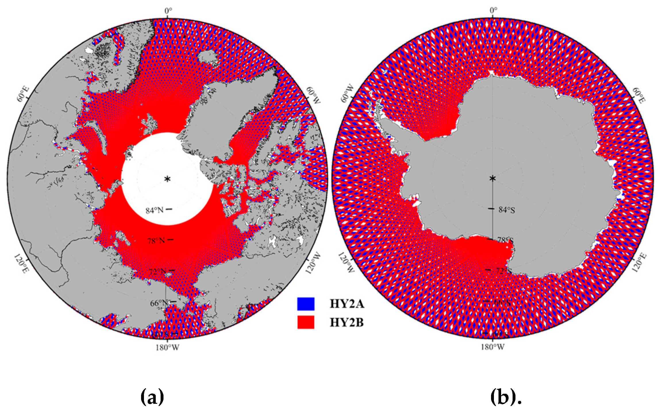
Figure 2 provides an example of the spatial coverage of the HY-2A/B in November 2018 in the Arctic and Antarctic regions. The month of November is considered to be the freeze-up period of the Arctic and the melt-out period of the Antarctic.
In this study, the data from 1st to 30th November 2018 were examined. The HY-2A/B ALT data had utilized approximately 470,000 surface points throughout all of November, respectively.
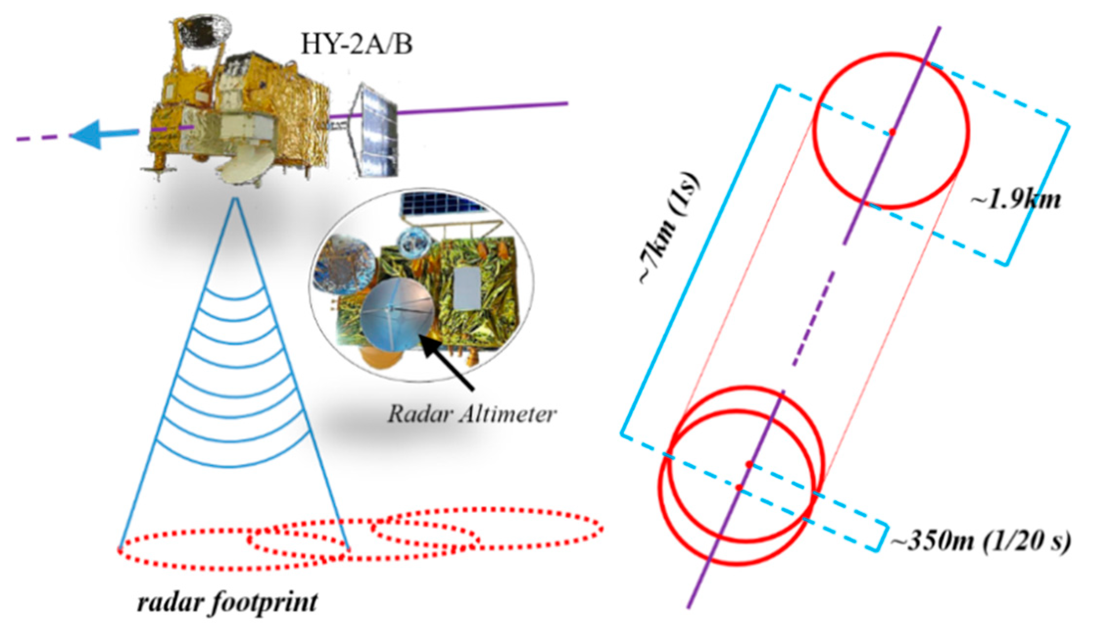
The ground footprint diameter of the Ku band of the HY-2A/B over the flat surfaces was 1.9 km, and the C band was approximately 10 km. Figure 3 showed the schematic diagram of the Ku band footprint of the HY-2A/B radar altimeters. The altimeter had continuously transmitted pulses to the ground. During the process, Millisecond-level pulse echo averaging was performed on the satellites. Then, the HY-2A/2B continuous measurements were separated by approximately 7 km along a track at 1 s intervals.
2.2. Other Data
2.2.1. HY-1C CCD Coastal Zone Imager (CZI)
Data source: The National Satellite Ocean Application Service (NSOAS). The HY-1C has five main payloads onboard, namely, a Chinese Ocean Color and Temperature Scanner (COCTS), Coastal Zone Imager, ultraviolet imager, calibration spectrometer, and an AIS system for ship tracking. The NSOAS provides the L1A level data of the HY-1C CZI, and these data were downloaded from the website: https://osdds.nsoas.org.cn/#/. The spatial resolution was set as 50 m.
2.2.2. OSISAF ICETYPE
Data source: The European Organization for the Exploitation of Meteorological Satellites (EUMETSAT) Ocean and Sea Ice Satellite Application Facility (OSI-SAF). The dataset provided four classification types in the Arctic region as follows: 1. No ice or very open ice; 2. Relatively young ice; 3. Ice that survived a summer melt; 4. Ambiguous ice type. The four classification types were assigned from the atmospherically corrected SSMIS brightness temperature and ASCAT backscatter values using a Bayesian approach. All of the sea ice types in the Antarctic were set as ambiguous ice. The spatial resolution was 10 km.
2.2.3. Sentinel 1a/b
Data source: The Technical University of Denmark (DTU). The 3-day Sentinel 1a/b mosaic product (1 km) of the Arctic and Antarctic regions were accessed from the website: http://www.seaice.dk/. The single scene of the Sentinel 1a/b (.jpg) could also be downloaded from the website with a spatial resolution of between 100 m and 1 km.
2.2.4. AARI Ice Chart
Data source: The weekly ice chart of the Russian Arctic and Antarctic Research Institute (AARI). The institute’s ice charts are based on the automatic generalization of regional ice charts which are compiled based on the analyses of satellite (visible, infra-red, and radar) information and reports from coastal stations and ships [21]. The ice charts provide the ice concentrations of the Antarctic region which this study download for free the website: http://www.aari.ru/.
3. Characteristics of the Waveforms
3.1. Contrasts between the Features of the Typical Waveforms in the Polar Regions
As can be seen in Figure 4, the rate of the 20 Hz data had been used in this study to show the typical waveforms of the different surface types (seawater and sea ice). The selected waveforms were mainly located in the Chukchi Sea and the Beaufort Sea. The ice in those locations were almost exclusively the first-year ice formations.
In the present study, the typical waveforms of the sea ice and seawater from the HY-2A/B ALT were found to be similar of the research result of Laxon [6,7], with the exception the C band. The echo presented a trend of first increasing and then decreasing, as detailed in Figure 4B. The trailing edge slopes of the diffuses surfaces were more slowly reduced than those of the quasi-specular surfaces. In addition, there were spiky waveforms of rapid rising and falling observed for the quasi-specular surfaces. Furthermore, major differences between the sea ice and seawater of the Ku and C Bands of the HY-2A/B had been presented, as shown in Figure 3 (C1 to C4).
3.2. Contrasts between the Different Tracking Packages
The trackers on the satellites had adopted different tracking algorithms for the various targets. For example, in the ERS-1, two different models (a seawater model and a sea ice model) were used. An SMLE was used for the seawater model, and an OCOG was used for the no-oceanic surfaces [22]. The HY-2A/B provided the data for the two different tracking packages as they also used two different methods.
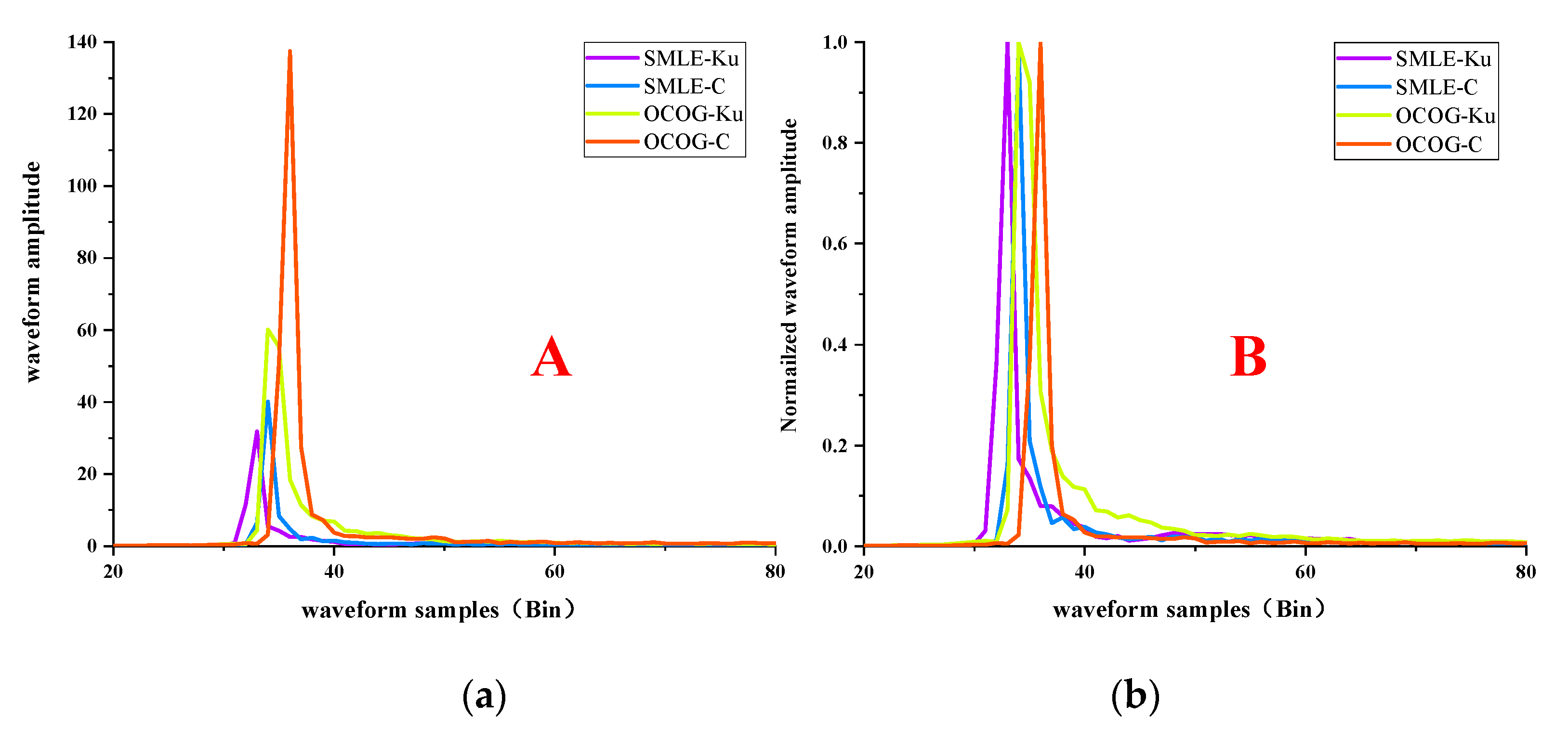
Figure 5a,b show the typical waveforms of the quasi-specular surfaces. The two different tracking algorithms had both maintained the waveform characteristics of the quasi-specular surfaces. It was observed that the maximum value of the OCOG was larger than that of the SMLE. Meanwhile, the maximum value of the C band was larger than that of the Ku Band.
As can be seen in Figure 6, the tracking results of the two tracking algorithms were similar. Both had maintained the waveform characteristics of the diffuse surfaces, and only minimal differences were observed between the SMLE and OCOG. However, the trailing edge slopes of the Ku Band were found to be greater than those of the C Band.
3.3. Classifying Parameters
Automatic gain control (AGC): An automatic gain control (AGC) method was used to ensure that the height of the plateau was adjusted in order to remain constant during the measurement processes.
Pulse peaking (PP): The pulse peaking was the ratio of the maximum sample value in the return echo to the power value in an individual sampler. The usage of the PP values was first proposed by Laxon (1994b) as a sea ice mapping technique. Since that time, many researchers have used the PP values for the sea ice classifications of radar altimeters [23,24,25,26,27]. The PP values also can be used to extract seawater and sea ice information. In the present study, the parameters were improved by ignoring the noise prone areas of the two measurements in 128 bins as follows:
where denote the values of the pulse peaking, max(Power) is the maximum sample value in the return echo from bin 21 to bin 108; and Power(i) is the power value in an individual sampler.
3.4. Contrasts in the Parameters
In the current research study, 1 Hz data were used to obtain the statistical law, which had a similar spatial resolution dataset for the verifications. It was found that the spatial resolution of the 20 Hz data was too high to accurately determine the matching data to complete the verifications.
3.4.1. Analysis of the 1 Hz Data
This study used the daily OSI-SAF_ICETYPE dataset in order to determine the ice types of the locations at the 1 Hz data points which matched the geographic information. The ice have three classification types: 1—young ice (sea ice of not more than one winter’s growth; in later sections, the AARI ice chart provide an ice type “first year ice” which also been defined as ”young ice” in this study); 2—old ice (sea ice that has survived at least one summer’s melt; the ice type of OSI-SAF_ICETYPE dataset called ”ice that survived a summer melt”); 3—ambiguous ice type.
The Arctic regions:
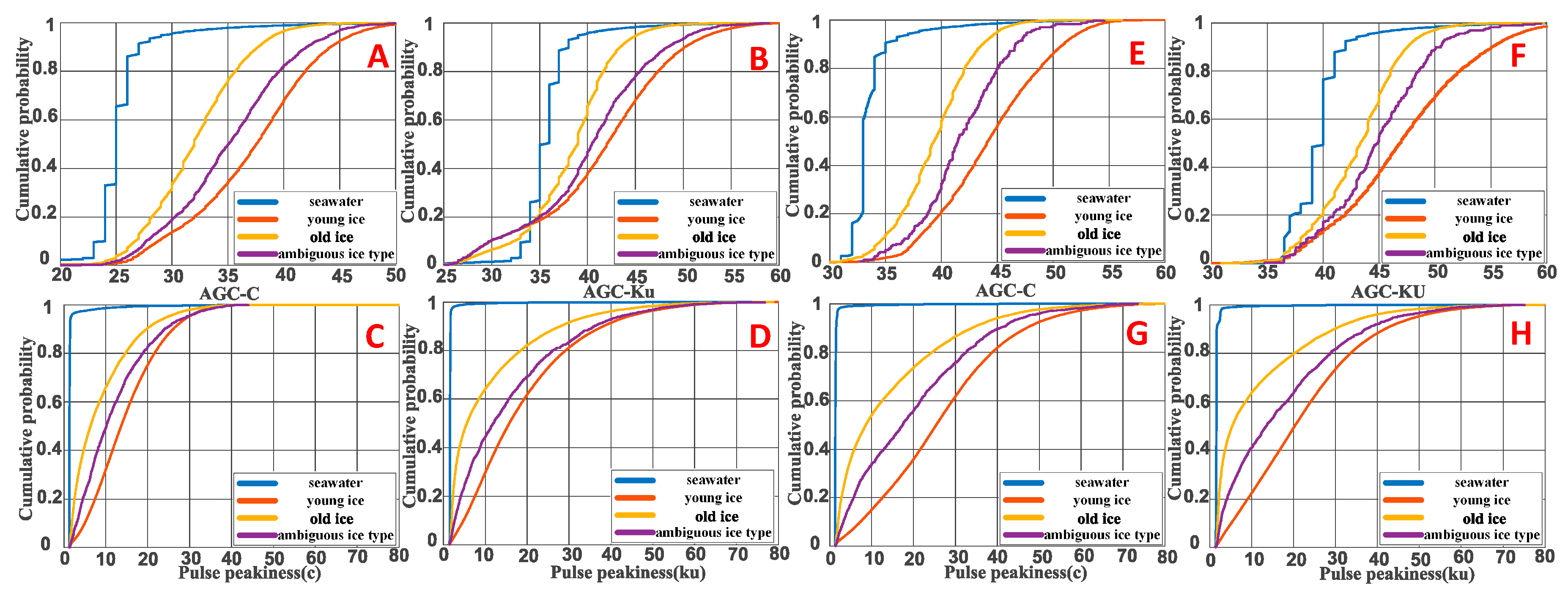
The cumulative probability distributions of each parameter and case are shown in Figure 7. In this study, the four waveform parameters were calculated as follows: AGC of the C Band; AGC of the Ku Band; PP of the C Band; and the PP of the Ku Band. It was found that the more separated the distributions were from one type to another, the easier it was to identify their flags.
Figure 7A–H showed that the distributions for all of the four parameters for the young ice, old ice, and ambiguous ice had closely resembled each other within the classes. However, the distributions for the open ice (for example, no ice or very open ice which were the same as seawater) had largely differed from the three ice types. The seawater had taken up a large portion of the low values of the AGC and PP. Additionally, the spread of the two parameters for the ice types was wide. Figure 7A,B,E,F showed that the AGC for the seawater and three ice types had overlaying areas. The AGC of the Ku Band from the HY-2A ALT was found to be particularly outstanding. The values from the overlay areas had resulted in errors when used for the classification process.
Since the three ice types were found to be similar to each other, the relatively young ice, ice that survived a summer melt, and ambiguous ice types were categorized as one type in this study.
It was found in this study that the values of the ice had a wide range (Figure 8). However, the distributions of seawater were very close. The overlaying areas of the AGC from the C Band were determined to be less than those of the Ku Band. The AGC values from the Ku Band of the seawater were almost included in the value range of the sea ice. Additionally, the AGC value of the C Band of the seawater were mainly less than 35. Meanwhile, that of the seawater was consistently larger than 35. The sea ice and seawater were found to be well separated by the PP values of the three types, as detailed in Figure 8A,B,E,F.
The Antarctic regions:
Figure 9 showed the cumulative probability distributions for the four different ice types for the four waveform parameters. In the Antarctic, the two different parameters were found to have good discrimination results for the seawater and sea ice. In Figure 9A,B,E,F, the seawater and sea ice have a largely overlap in the region of low value. However, there were less overlap in Figure 9A,B,E,F. These AGC values of overlapping areas has an influence on separate the sea water and sea ice. The PP values were determined to be more effective than the AGC for the classification process. It was observed at low value regions of the PP that the cumulative probability of the seawater had almost reached as high than 90%, and the rate of sea ice was very low.
In Figure 9B,F, the values of Ku Band’s AGC from the two different surfaces had displayed coincidence between them. However, those of the C Band had not.
3.4.2. Analysis of the 20 Hz Data
This study selected some visible and SAR data of the northern and southern polar regions to examine.
Previously, Peacock [23] had used the pulse peak (PP) values of 1.8 to make distinctions between the diffused and quasi-specular echoes of ERS-1. He found the main source of the diffused echoes were seawater or ice floe surfaces. The quasi-specular echoes had originated from the sea surfaces in areas with high ice concentrations. In another related study, Knudsen [28] believed that the threshold of 1.8 could be used to classify the two different surfaces.
The pulse peak values were used in this study also. For the research of 1 Hz and above, the PP values were found to have high recognition. In the analysis of the 20 Hz data, a value of 3 was set as the threshold. The waveforms with PP values less than 3 were processed as a type of diffused waveform, and those with PP values greater than 3 were processed as quasi-specular waveforms. The average type of waveform with PP values greater than 3 were spike-like waveforms. Meanwhile, those with PP values less than 3 were “ocean like” waveforms.
The Antarctic regions:
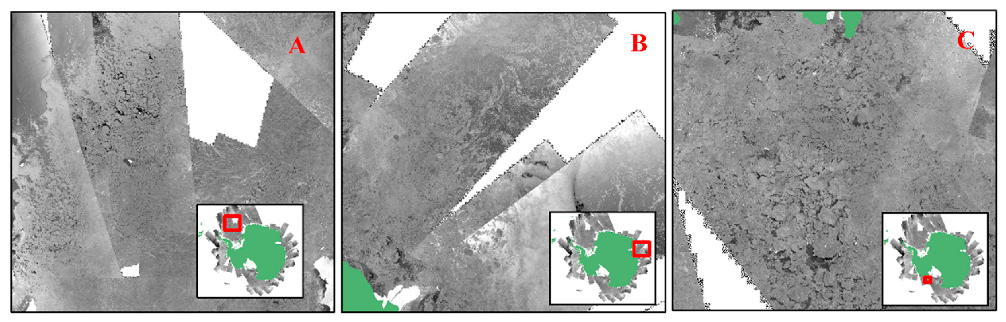
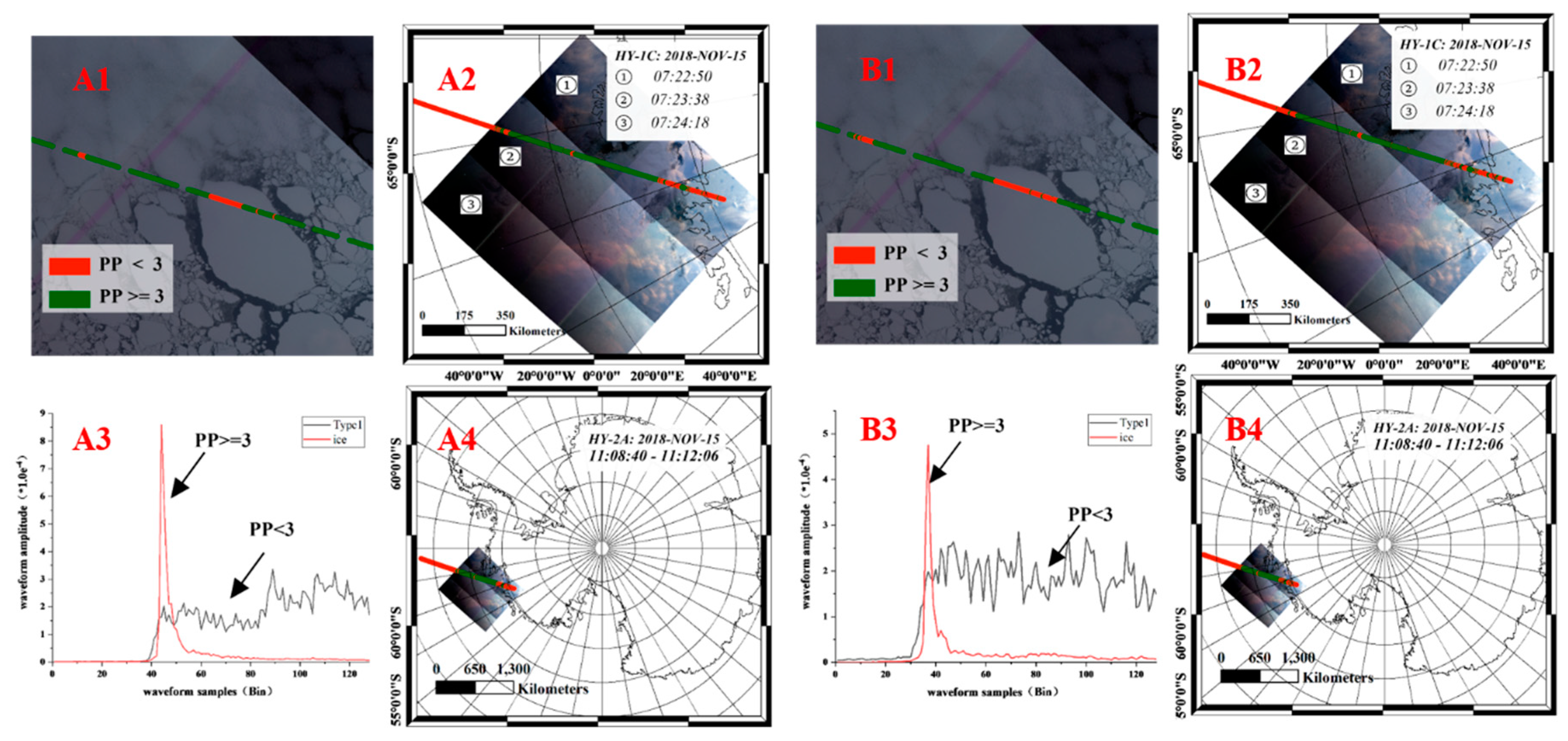
The impacts of the orbit and clouds could not be ignored in this study. Therefore, the less visible remote sensing data from the HY-1C from November were selected. The data from the HY-1C are shown in Figure 10 and Figure 11, in which the intervals between the HY-2A/B ALT were simultaneously less than 5 h.
The PP values of the small pieces of ice were found to be greater than 3. Also, in the leads near shore and the large ice floe centers, there were some cases where the PP values were greater than 3. The two different types of waveforms were above the ice sheet.
In Figure 11, the HY-2B had results similar to those of the HY-2A. The HY-2A ALT data had indicated PP values less than 3 in the regions of small contiguous ice floes. The data of these regions had displayed spike-like waveforms. In the centers of the large ice floes, “ocean like” waveforms had existed.
Although the footprint of the C Band was larger than that of the Ku Band, the C band was also correctly flagged on the same larger ice floes which had been identified as the diffuse surfaces in the Ku Band. However, there were found to be small differences in the number of identifications.
The Arctic regions:
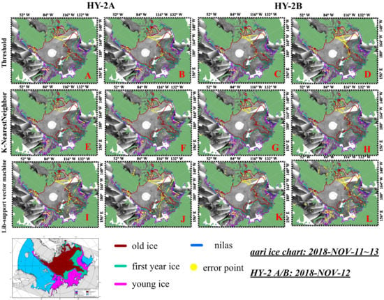
This study selected the altimeter data from the HY-2A/B for 15 November 2018 as an example. The data of the AARI ice charts were from 11–13 November 2018. The chart (Figure 12C) provided five types of ice as follows: 1—Nilas (ice rind); 2—Young ice; 3—First-year ice; 4—Old ice (had survived at least one summer melt).
The old ice was found to be the very similar to the old ice which had been identified in the OSI-SAF ICETYPE dataset.
It was determined in this study that the PP values were lower than 3 from the seawater areas not only in the C Band, but also in the Ku Band. The PP values from the young ice and first-year ice were found to be greater than 3. However, above the old ice, there were some places where the PP values were less than 3 (Figure 12A,B). In Figure 12D,E, the “ocean like” echoes of the band C and Band Ku had existed in the regions of old ice. But these echoes from different band in Arctic and Antarctic had a slight difference in position. In the edges of sea ice (Figure 12F,G), the PP values from some nilas were less than 3 whose waveform similar to seawater. Due to finger rafting of the thin sheets, nilas ice usually have roughness surface [29].
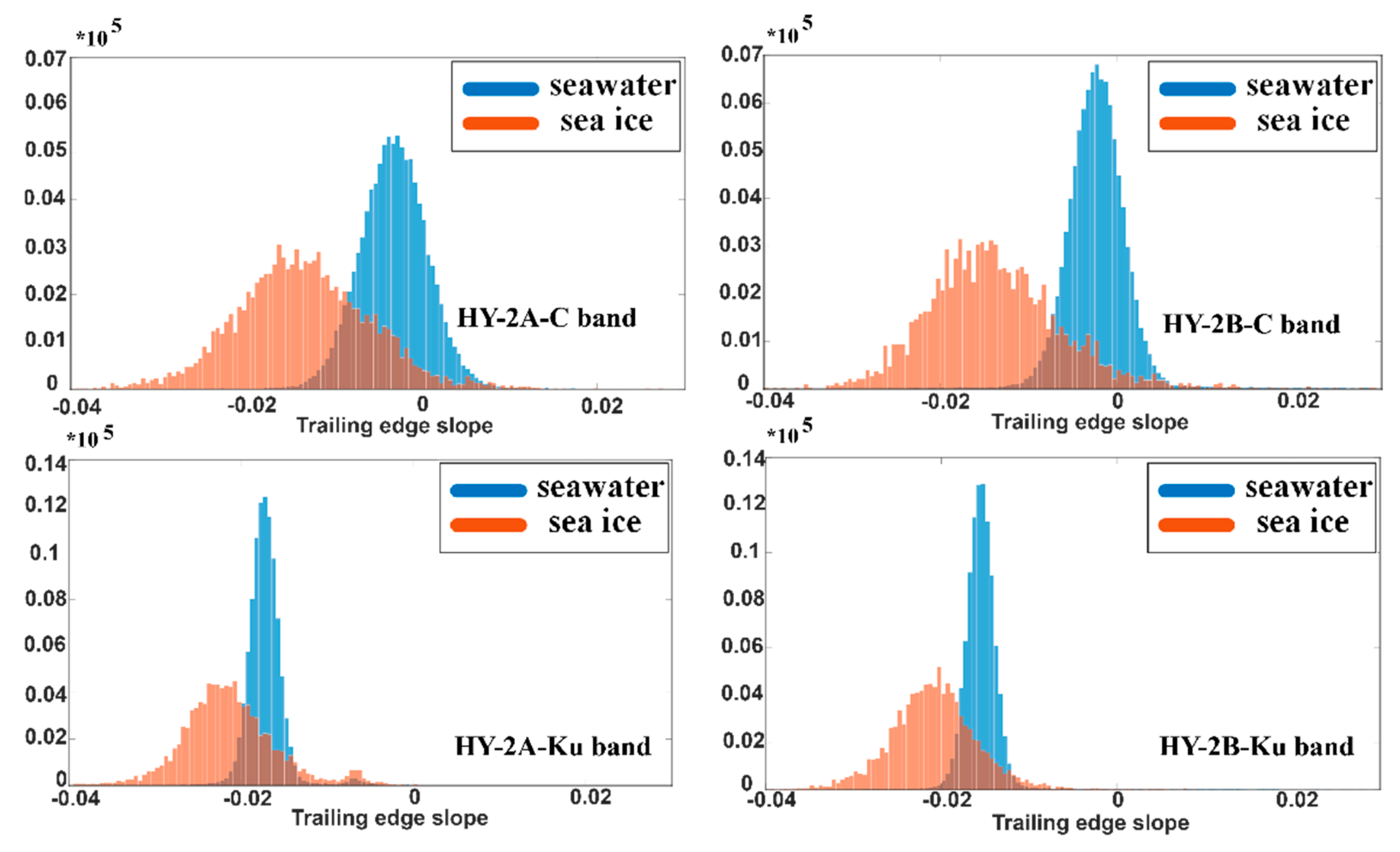
In Figure 13, the average waveforms of the data from the old ice with PP values less than 3 and the average waveforms of the seawater are shown.
By comparing Figure 13a with Figure 13b, it could be seen that the trailing edge slopes of the old ice were greater than those of the seawater. Meanwhile, the trailing edges of the seawater from the C Band were almost parallel to the axis. In contrast, the trailing edges of the old ice were not.
This study fitted the trailing edges of the aforementioned waveforms using a least square method and the statistical data of the slopes were obtained, as shown in Figure 14.
The average waveforms of the old ice with PP values less than 3, along with those of the seawater, had presented significant differences in regard to their trailing edges. Meanwhile, the single waveforms were not found to be significantly different. As shown in Figure 14, there were many overlapping regions of seawater and old ice (PP > 3). Furthermore, there were many effects observed in the trailing edges which had resulted from the directional angles, physical properties in the scattering cells, and the noise of the echoes. It was found in this study that those effects could not be ignored in the 20 Hz data.
4. Classification Process
In the present study, since there were no matching data for the validation of the 20 Hz data, only the 1 Hz data were classified. First, quality control measures were carried out in which the land was masked and the incorrect tracking data were removed.
The classification rate calculation formula used in this study had first been identified by Zygmuntowska [24], and was calculated as follows:
where denoted the classification accuracy of the classification algorithm, ; classification results of the classification algorithm, were the classification results of the data used for the verification process; and the OSI-SAF ICETYPE dataset was adopted as the validation data.
4.1. Threshold Segmentation
The HY-2A/B’s AGC and PP values were used for comparison purposes in order to draw the scatter plots, as shown in Figure 15.
In Figure 15, the distributions of the PP values from the seawater appear to be dense. However, that was not the case for the sea ice. The PP values of the sea ice were observed to be greater than those of the seawater. In addition, there was major overlapping of the AGC from the two different surfaces. In the Antarctic regions, the data range of the PP values from the seawater were determined to be larger than that of the Arctic regions.
It was found in this study that the small values of the AGC from the HY-2A had many discrete values. These small values existed at the joints where the two tracking packets switched. However, this had not occurred in the HY-2B. Therefore, the improvements of the HY-2B instrument had been demonstrated in the results of this study.
Therefore, in accordance with the findings detailed Section 3.4.2, along with other previous related sections, this study selected the PP values the parameters of the classification threshold. The threshold values were then set, as detailed in Table 2.
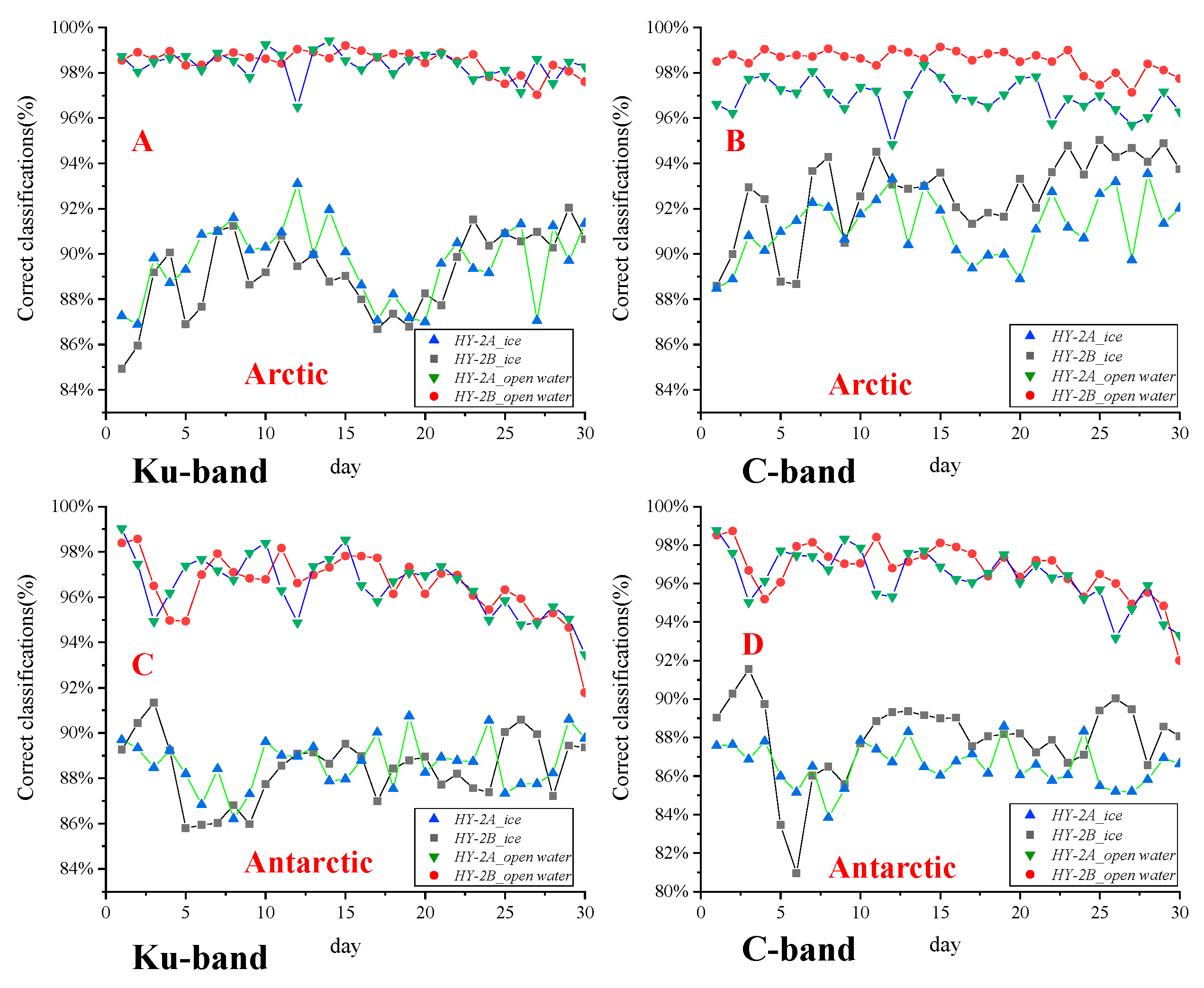
Results of the daily classification were shown in Figure 16. Figure 16A,C showed the results of the Ku band from HY-2A/B, meanwhile Figure 16B,D showed the results of C band form HY-2A/B. Comparing the accuracy of the two different places, the accuracy rates of the Arctic regions changed in a smaller rang than the Antarctic regions. It was observed in the daily classification of the November data that a high level of accuracy had been maintained. Generally speaking, the accuracy level for the sea ice was higher than that for the seawater.
It was found that a simple threshold segmentation with a single parameter could also achieve a high accuracy rate (Table 3), and there were small differences observed between the HY-2A ALT and HY-2B ALT data. Comparing the result of sea ice and seawater in Table 3, the average accuracy rates of the seawater for threshold segmentation were higher than 96% both in Arctic and Antarctic. However, the average accuracy rates of the sea ice were lower than 90% except band C from HY-2B ALT in arctic.
4.2. K-Nearest-Neighbor (KNN)
The data from November 1st to 10th were used to build the model of this study’s classification method (KNN, Lib-svm). The data from 11–30 November were adopted as the validation data. This study chose four parameters for the classifications: AGC and PP values from the C Band and Ku Band, respectively.
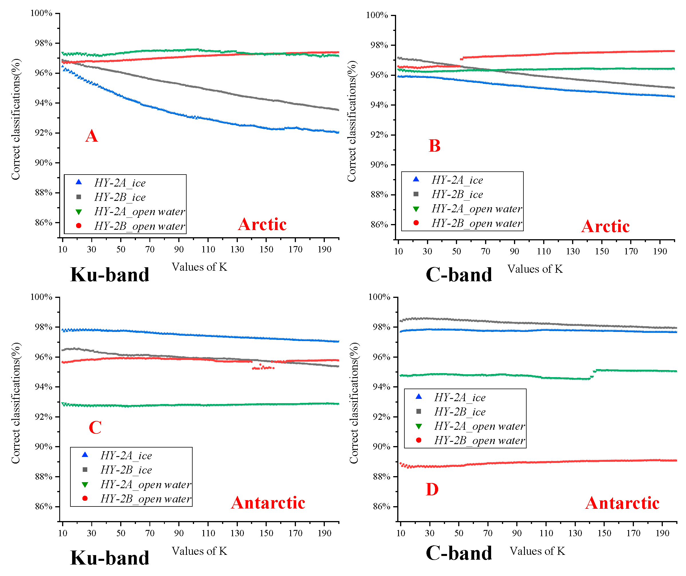
The principle of the KNN involved the statistical accuracies of the adjacent areas. Therefore, the K (number of selected points in the adjacent areas) had impacted the results. In this study, K was set in the range of 10 to 200.
In Figure 17, all the accuracy rates are greater than 80%. The overall accuracy of the two different bands from the two different satellites had remained within a stable change range, with the exception of the Ku Band in the Arctic regions. In the Antarctic regions, the classification accuracy rate of the seawater was observed to be relatively lower than the others.
4.3. Lib-Support Vector Machine (LibSVM)
In this study, a support vector machine pattern recognition software package which had been developed by Chih-Jen Lin was utilized. The code was a free download from the website: (http://www.csie.ntu.edu.tw/~cjlin/ libsvm). This study also chose the AGC and PP values from the C and Ku Bands for the classification process. The results are shown in Table 4.
The classification accuracy rates of the Antarctic seawater were found to be low. However, the data for the Arctic region had also provided an accuracy similar to the KNN and threshold segmentation.
5. Discussion
The two different track algorithms (OCOG and SMLE) were incorporated in parallel in the HY-2A/B ALT in order to prevent unlocked tracking above the no-oceanic surfaces. As detailed in Figure 5 and Figure 6, the echoes from the seawater all had basic characteristics. For example, the spike-like waveforms’ maximum from the sea ice of the OCOG was greater than that of the SMLE. Although there were differences in the waveform amplitudes between the two different packages, it was found that the shapes of the waves could be used to examine the separations between the sea ice and seawater in the polar regions.
In previous studies, many researchers had used airborne altimeters to obtain their results [24]. They found that the echoes from old ice had smaller trailing edge slopes than the echoes from young ice. The results of this study were similar to the previous findings. However, not all of the echoes from the HY-2A/B for the old ice were observed to display the aforementioned phenomenon. As shown in Figure 12, spike-like echoes had existed in the regions of old ice, with the exception of the “ocean-like” echoes. The biggest differences between the radar altimeters used by Zygmuntowska and Drinkwater were that the footprints on the ground were much smaller than the ground footprint of the HY-2A/B ALT. In addition, the sources of the signals for the bigger footprint were more complicated than those for the smaller footprint. For example, the echoes were a mixture of signals from many different types of ice in the footprint. In the Antarctic region, “ocean-like” waveforms had existed in the centers of the large ice floes. Although the footprint of the C Band was larger than that of the Ku Band, the C Band had been correctly flagged on the same larger ice floes which had been identified as a diffuse surfaces in the Ku Band. The difference was the number of identifications.
The attenuations of the echoes from the Ku Band were greater than those of the C Band above the ocean surface. The averages of the diffused echoes in the regions of the old ice were similar to that of the seawater. However, the trailing edges of the seawater from the C Band were found to be almost parallel to the axis, and the trailing edges of the diffused echoes in the regions of old ice were not. Also, there were many effects of the trailing edges observed, which had resulted from the direction angles, physical properties in the scattering cells, and the noise of the echoes. These effects could not be ignored by using a simple least square fitting method for the trailing edges. Meanwhile, the research results had provided a basis for the study of re-tracking algorithms for the altimeters of the HY-2A/B ALT.
Based on the previous analysis of the echoes, three methods (threshold segmentation, KNN, and LIBSVM) were presented with four waveform parameters (AGC and PP values of the Ku and C Bands) in order to distinguish between sea ice and seawater in the polar regions in Section 4.
The accuracy rate of the LIBSVM was found to be the lowest of the three methods in both the Arctic and Antarctic regions. The KNN Method was able to maintain a stable high accuracy rate with the different K values, and the single parameter threshold segmentation was determined to also have a good accuracy rate.
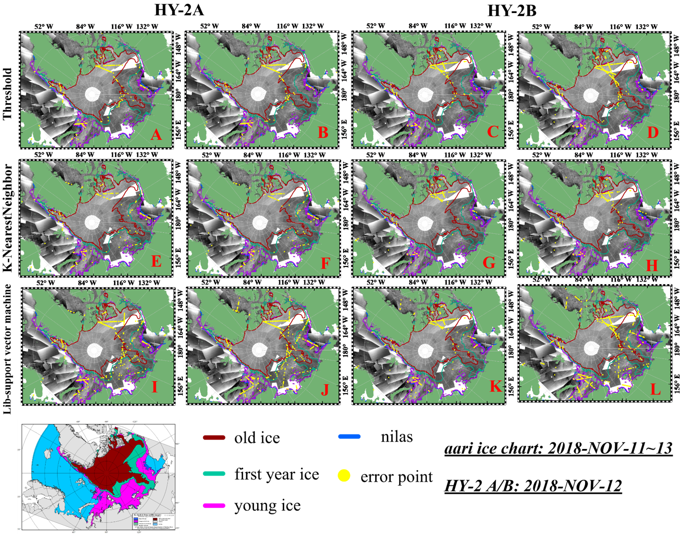
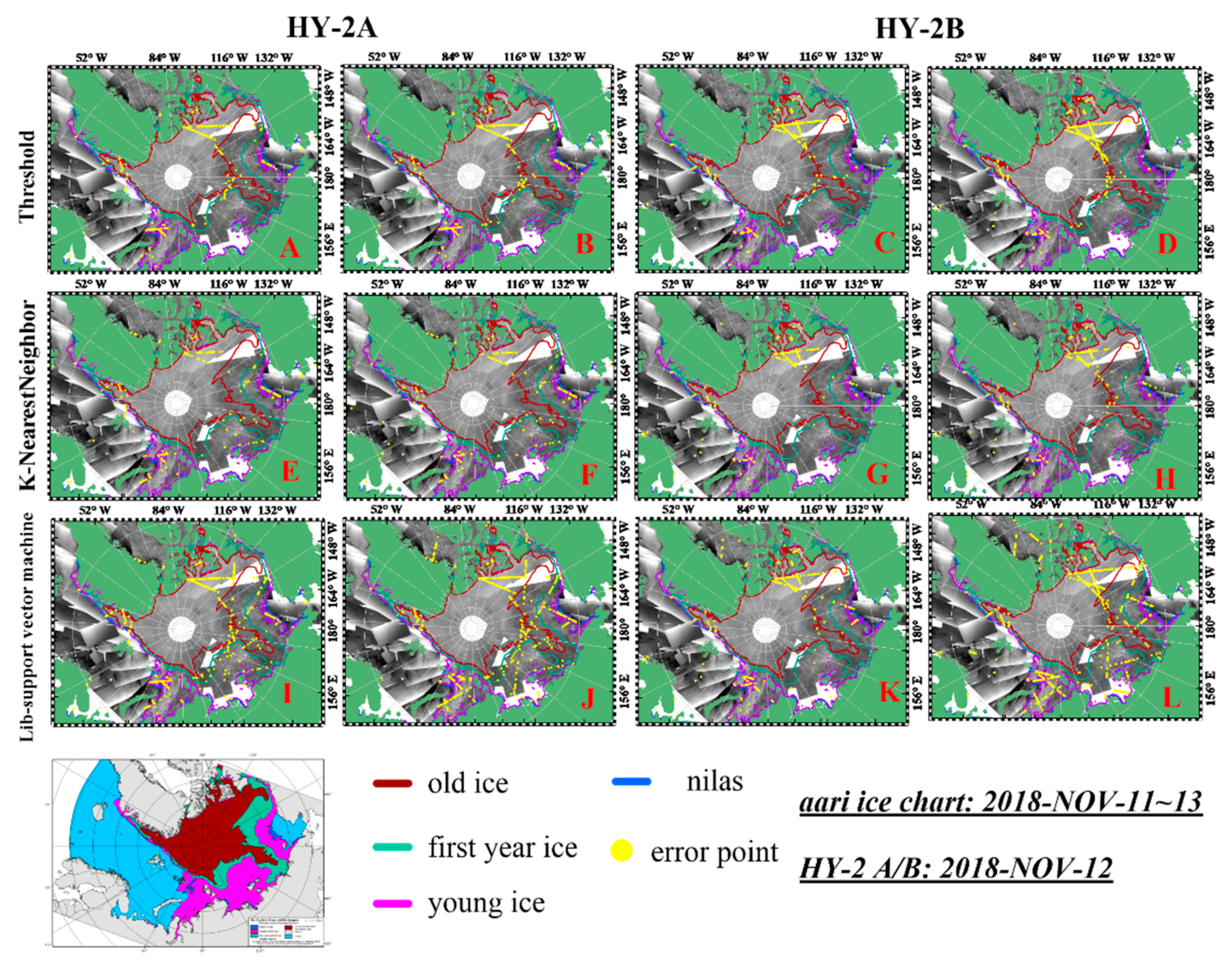
For the purpose of discussing the distinguishing results of the three examined methods, the error points of results and OSI-SAF are plotted in Figure 18 and Figure 19. In the figures, the previously mentioned ice chart was utilized to correct the results of the classifications.
The AARI ice chart for 11–13 November of the Arctic region, and the ice chart for 15 November of the Antarctic region, were used in this study as references. The error points of the Arctic regions were mainly located in the old ice around Queen Elizabeth Island. The areas where the error occurs were consistent with the positions of the ‘ocean-like’ waveforms. The error distribution of LIBSVM was the most dispersed. The errors of the KNN had occurred near the old ice and sea ice boundaries. The diffused echoes from the old ice were found to be similar to those of the seawater.
In the Antarctic regions, an almost complete correct identification of the seawater had been achieved in the areas with no ice using the KNN with the threshold method. However, there were many misclassifications in areas with sea ice, as illustrated in Figure 19. It was found that the noise from the ice floes had impacted the classification results. Since November was the summer season in the Antarctic regions at the local time, the ice had been melting. The errors of the threshold were found to be mainly distributed in the areas containing many sea ice floes, as illustrated in Figure 20 (Weddell Sea, Pulitzer Sea, and Ross Sea).
In the present study, it was found that the results of the LIBSVM were so inaccurate that the errors had been distributed in all of the orbits of the Antarctic regions. In addition, in the large footprint of the altimeter, there tended to be a large number of non-singular ground signals which had introduced many mixed signals. Meanwhile, it was also determined that the OSI-SAF ICETYPE dataset was not exactly correct. The spatial resolution of the dataset was 10 km, which was far greater than the sizes of the ice floes. Therefore, it was not able to accurately present the distributions of the ice floes. The large footprints only allows a detection of large-scale changes in surface structure and signal strength. This further limits the possibility of distinguishing between surface types. A more detailed study is needed to analyze the impact of the different resolutions as well as the influence of snow and roughness on the HY-2A/B ALT echoes.
The waveforms of radar altimeter are sensitive to the electrical properties [30] and surface roughness [31] and so on. Beaven [30] found that the snow influence on the reflected radar signals from the snow-ice interface can be neglected when the snow is dry and cold based on the laboratory experiments. The Arctic in November is winter, while the season is summer in the Antarctic regions. The environment of Antarctic was not as dry and cold as the Arctic in November. The Antarctic sea ice had been melting in November. Willatt [32] further found the dominant scattering surface was not always the snow-ice interface for the Antarctic sea ice surveyed based on a sled-borne radar during the summer seasons. The mean depth of the dominant scattering surface of the radar was only around 50% of the mean measured snow depth. Thus, the snow depth has a not negligible influence on the formation of “ocean-like” echoes in the centers of the large ice floes. Due to the melting processes, the ice in the Antarctic low sea ice concentration was very loose. From the scale of the altimeter footprint, the surface of these areas is not so smooth. The snow cover and the changes in the surface roughness of the ice zones generate a significant difference in the echoes. These influences brought difficulties to the separation of sea ice and seawater in the Antarctic. Meanwhile, there are differences between the echoes of band C and band Ku (Figure 10, Figure 11 and Figure 12). The band C and Ku have different abilities to penetrate snow and ice as they have different wavelengths. In Figure 12D,E, the “ocean-like” echoes of the Band C and Band Ku had existed in the regions of old ice. Meanwhile, these echoes from different bands had a slight difference in position in the Arctic and Antarctic.
6. Conclusions
In the present study, HY-2A/B altimeter L1b data over the polar regions were analyzed. The differences between the SMLE and OCOG tracking packages were analyzed using the waveform results. It was found that the different tracking packages could maintain the waveform characteristics of the diffuse and quasi-specular surfaces. Those characteristics were then utilized in this study for classification purposes.
The echoes from the seawater areas were found to be diffuse type echoes. The echoes from the sea ice in the Arctic region were observed to be mainly quasi-specular type echoes. It was found that some “ocean-like” waveform data had existed in the old ice areas. In the Antarctic regions, the center surfaces of the large ice floes were determined to be diffuse surfaces. At the same time, specular reflections and diffuse reflections were found to exist on the surfaces of the shelf ice covers, and the diffuse reflections were dominant. In addition, there were differences observed between the echoes from the seawater areas, and also from the diffused echoes obtained from the old ice. These observed differences could potentially provide the basis for the future study of re-tracking algorithms for the altimeters of the HY-2A/B ALT.
The accuracy rate of the separation results for the LIBSVM except Band Ku from HY-2B ALT was found less than 40% in Antarctic. Meanwhile, the other two methods had on average demonstrated 80% correct detections of the waveforms. The errors of LIBSVM had mainly occurred in the extractions related to the seawater areas. All of the incorrectly distinguished results of the three methods were observed to be located in the regions of the old ice. The incorrectly distinguished results were found to be related to the “ocean-like” waveforms. Those waveforms were similar to the seawater areas. It was also found that the AGC and PP values had displayed fewer differences between the two surfaces. An additional factor which may have impacted the results was the fact that the sea ice had been melting in November (summer season in the Antarctic region), and a large number of ice floes and leads had appeared. Therefore, a large number of non-singular ground signals in the footprint had been received by the instrument. These ground signals had resulted in increasing the difficulty in distinguishing the seawater from the sea ice.
In conclusion, it was determined in this study that the HY-2A/B had the ability to accurately classify sea ice and seawater. Furthermore, in accordance with the statistical results of the parameters mentioned above, the data quality of the HY-2B altimeter had displayed obvious improved results when compared with those of the HY-2A altimeter.
In the study, we just had the data of November 2018 (HY-2B has not been running for a whole year). We will analyze differences between the different seasons from a geophysical perspective after the HY-2B operates for a whole year. Meanwhile, since there were fewer data used to distinguish the 20 Hz data for validation, there were found to be some deficiencies in the analysis of the 20 Hz data in this study. In future research, more detailed analyses of the 20 Hz data will be carried out.
Author Contributions
All authors contributed to the conceptualization; C.J. performed the formal analysis and original draft writing; M.L. and H.W. contributed to the supervision; all authors contributed to the paper.
Funding
This work was supported by National Key R&D Program of China under Project 2016YFC1401000; and the National Natural Science Foundation of China under Grant 41876204 and 41630969.
Acknowledgments
This work is supported by National Satellite Ocean Application Service, State Oceanic Administration. We want to thank EUMETSAT for providing the icetype product, and DTU for providing the data of Sentinel 1a/b. The authors would also like to thank Youguang Zhang, Yongjun Jia, Tao Zeng, Jing Ding and Lijian Shi for the help of data processing.
Conflicts of Interest
The authors declare no conflict of interest.
Abbreviations
The following abbreviations are used in this manuscript:
| AAGS | Average attitude/specular gate |
| AARI | Russian Arctic and Antarctic Research Institute |
| AGC | Automatic gain control |
| AIS | the global ship automatic identification system |
| ALT | Altimeter |
| ASCAT | Advanced Scatterometer |
| CNSA | the China National Space Administration |
| COCTS | Chinese Ocean Color and Temperature Scanner |
| CZ 4 | Chang Zheng 4 (CZ meaning “Long March”), The Long March 4 is a Chinese three-stage, liquid-propellant orbital launch vehicles. |
| CZI | Coastal Zone Imager |
| DCS | the marine buoy measurement data collection system |
| DTU | the Technical University of Denmark |
| ENVISAT | European Space Agency Environmental Satellite |
| ERS-1/2 | European Remote Sensing satellite-1/2 |
| GDR | Geophysical Data Records |
| GEOS-3 | Geodynamics Experimental Ocean Satellite 3 |
| HY-2A/B | Haiyang – 2 A/B, the Chinese Marine Dynamic Environment Satellites, Haiyang meaning “Marine” |
| IGDR | Interim Geophysical Data Records |
| KNN | K-nearest-neighbor |
| LIBSVM | Lib-support vector machine |
| MCT | the model compatible tracker of altimeter |
| NSOAS | the Chinese National Satellite Ocean Application Service |
| OCOG | Offset Center of Gravity |
| OSI-SAF | the European Organization for the Exploitation of Meteorological Satellites (EUMETSAT) Ocean and Sea Ice Satellite Application Facility (OSI-SAF). |
| PP | Pulse peaking |
| SAR | Synthetic aperture radar |
| SGDR | Sensor Geophysical Data Records |
| SMLE | Suboptimal Maximum Likelihood Estimation methods |
| SSMIS | Special Sensor Microwave Imager/Sounder |
References
- Untersteiner, N. The Global Climate; Cambridge University Press: New York, NY, USA, 1984; pp. 260–287. [Google Scholar]
- Shokr, M.; Sinha, N. Sea Ice: Physics and Remote Sensing; John Wiley & Sons: Hoboken, NJ, USA, 2015. [Google Scholar]
- Dwyer, R.; Godin, R. Determining Sea-Ice Boundaries and Ice Roughness Using GEOS-3 Altimeter Data; Technical Report; NASA Wallops Flight Center: Wattsville, VA, USA, 1980.
- Rapley, C. First observations of the interaction of ocean swell with sea ice using satellite radar altimeter data. Nature 1984, 307, 150. [Google Scholar] [CrossRef]
- Laxon, S. Seasonal and inter-annual variations in Antarctic sea ice extent as mapped by radar altimetry. Geophys. Res. Lett. 1990, 17, 1553–1556. [Google Scholar] [CrossRef] [Green Version]
- Laxon, S. Sea ice altimeter processing scheme at the EODC. Int. J. Remote Sens. 1994, 15, 915–924. [Google Scholar] [CrossRef]
- Laxon, S. Sea ice extent mapping using the ERS-1 radar altimeter. Adv. Remote Sens. 1994, 3, 112–115. [Google Scholar]
- Rinne, E.; Similä, M. Utilisation of CryoSat-2 SAR altimeter in operational ice charting. Cryosphere 2016, 10, 121–131. [Google Scholar] [CrossRef] [Green Version]
- Shen, X.; Zhang, J.; Zhang, X.; Meng, J.; Ke, C. Sea ice classification using Cryosat-2 altimeter data by optimal classifier–feature assembly. IEEE Geosci. Remote Sens. Lett. 2017, 14, 1948–1952. [Google Scholar] [CrossRef]
- Chase, J.R.; Holyer, R.J. Estimation of sea ice type and concentration by linear unmixing of Geosat altimeter waveforms. J. Geophys. Res. Ocean. 1990, 95, 18015–18025. [Google Scholar] [CrossRef]
- Drinkwater, M.R. Ku band airborne radar altimeter observations of marginal sea ice during the 1984 Marginal Ice Zone Experiment. J. Geophys. Res. Ocean. 1991, 96, 4555–4572. [Google Scholar] [CrossRef]
- Giles, K.A.; Laxon, S.W.; Ridout, A.L. Circumpolar thinning of Arctic sea ice following the 2007 record ice extent minimum. Geophys. Res. Lett. 2008, 35. [Google Scholar] [CrossRef] [Green Version]
- Laxon, S.; Peacock, N.; Smith, D. High interannual variability of sea ice thickness in the Arctic region. Nature 2003, 425, 947. [Google Scholar] [CrossRef]
- Ridout, A.; Ivanova, N.; Tonboe, R.; Laxon, S.; Timms, G.; Kern, S.; Kloster, K. Algorithm Theoretical Basis Document; SICCI-ATBDv0-07-12 Version 1.1./03Sept 2012, Technical Report; ESA: Paris, France, 2012.
- Laxon, S.W.; Giles, K.A.; Ridout, A.L.; Wingham, D.J.; Willatt, R.; Cullen, R.; Kwok, R.; Schweiger, A.; Zhang, J.; Haas, C. CryoSat-2 estimates of Arctic sea ice thickness and volume. Geophys. Res. Lett. 2013, 40, 732–737. [Google Scholar] [CrossRef] [Green Version]
- Yu, Y.; Zhang, W.; Wu, Z.; Yang, X.; Cao, X.; Zhu, M. Assimilation of HY-2A scatterometer sea surface wind data in a 3DVAR data assimilation system—A case study of Typhoon Bolaven. Front. Earth Sci. 2015, 9, 192–201. [Google Scholar] [CrossRef]
- Lin, M.; Jiang, X. HY-2 ocean dynamic environment mission and payloads. In Proceedings of the 2014 IEEE Geoscience and Remote Sensing Symposium, Quebec City, QC, Canada, 13–18 July 2014; pp. 5167–5170. [Google Scholar]
- Pan, D.; Gong, F.; Chen, J. The Chinese environment satellite mission status and future plan. Proceedings of Sensors, Systems, and Next-Generation Satellites XIII. p. 747424. Available online: https://www.spiedigitallibrary.org/conference-proceedings-of-spie/7474/747424/The-Chinese-environment-satellite-mission-status-and-future-plan/10.1117/12.830251.full (accessed on 20 June 2019).
- Xu, K.; Jiang, J.; Liu, H. A new tracker for ocean-land compatible radar altimeter. In Proceedings of the 2007 IEEE International Geoscience and Remote Sensing Symposium, Barcelona, Spain, 23–28 July 2007; pp. 3825–3828. [Google Scholar]
- Musman, S.; Drew, A.; Douglas, B. Ionospheric effects on Geosat altimeter observations. J. Geophys. Res. Ocean. 1990, 95, 2965–2967. [Google Scholar] [CrossRef]
- Selyuzhenok, V.; Krumpen, T.; Mahoney, A.; Janout, M.; Gerdes, R. Seasonal and interannual variability of fast ice extent in the southeastern Laptev Sea between 1999 and 2013. J. Geophys. Res. Ocean. 2015, 120, 7791–7806. [Google Scholar] [CrossRef]
- Scott, R.; Baker, S.; Birkett, C.; Cudlip, W.; Laxon, S.; Mantripp, D.; Mansley, J.; Morley, J.; Rapley, C.; Ridley, J. A comparison of the performance of the ice and ocean tracking modes of the ERS-1 radar altimeter over non-ocean surfaces. Geophys. Res. Lett. 1994, 21, 553–556. [Google Scholar] [CrossRef] [Green Version]
- Peacock, N.R.; Laxon, S.W. Sea surface height determination in the Arctic Ocean from ERS altimetry. J. Geophys. Res. Ocean. 2004, 109. [Google Scholar] [CrossRef]
- Zygmuntowska, M.; Khvorostovsky, K.; Helm, V.; Sandven, S. Waveform classification of airborne synthetic aperture radar altimeter over Arctic sea ice. Cryosphere 2013, 7, 1315–1324. [Google Scholar] [CrossRef] [Green Version]
- Ricker, R.; Hendricks, S.; Helm, V.; Skourup, H.; Davidson, M. Sensitivity of CryoSat-2 Arctic sea-ice freeboard and thickness on radar-waveform interpretation. Cryosphere 2014, 8, 1607–1622. [Google Scholar] [CrossRef] [Green Version]
- Zakharova, E.A.; Fleury, S.; Guerreiro, K.; Willmes, S.; Remy, F.; Kouraev, A.V.; Heinemann, G. Sea Ice Leads Detection Using SARAL/AltiKa Altimeter. Mar. Geod. 2015, 38, 522–533. [Google Scholar] [CrossRef]
- Wernecke, A.; Kaleschke, L. Lead detection in Arctic sea ice from CryoSat-2: Quality assessment, lead area fraction and width distribution. Cryosphere 2015, 9, 1955–1968. [Google Scholar] [CrossRef]
- Knudsen, P.; Andersen, O.B.; Tscherning, C.C. Altimetric gravity anomalies in the Norwegian-Greenland Sea-Preliminary results from the ERS-1 35 days repeat mission. Geophys. Res. Lett. 1992, 19, 1795–1798. [Google Scholar] [CrossRef]
- Guest, P.S.; Davidson, K.L. The aerodynamic roughness of different types of sea ice. J. Geophys. Res. Ocean. 1991, 96, 4709–4721. [Google Scholar] [CrossRef] [Green Version]
- Beaven, S.; Lockhart, G.; Gogineni, S.; Hossetnmostafa, A.; Jezek, K.; Gow, A.; Perovich, D.; Fung, A.; Tjuatja, S. Laboratory measurements of radar backscatter from bare and snow-covered saline ice sheets. Remote Sens. 1995, 16, 851–876. [Google Scholar] [CrossRef]
- Brown, G. The average impulse responce of a rough surface and its applications. IEEE J. Ocean. Eng. 1977, 2, 67–74. [Google Scholar] [CrossRef]
- Willatt, R.C.; Giles, K.A.; Laxon, S.W.; Stone-Drake, L.; Worby, A.P. Field investigations of Ku-band radar penetration into snow cover on Antarctic sea ice. IEEE Trans. Geosci. Remote Sens. 2009, 48, 365–372. [Google Scholar] [CrossRef]
Figure 1.
Differences in the radar altimeter returns over the diffuse and quasi-specular surfaces [6,7].
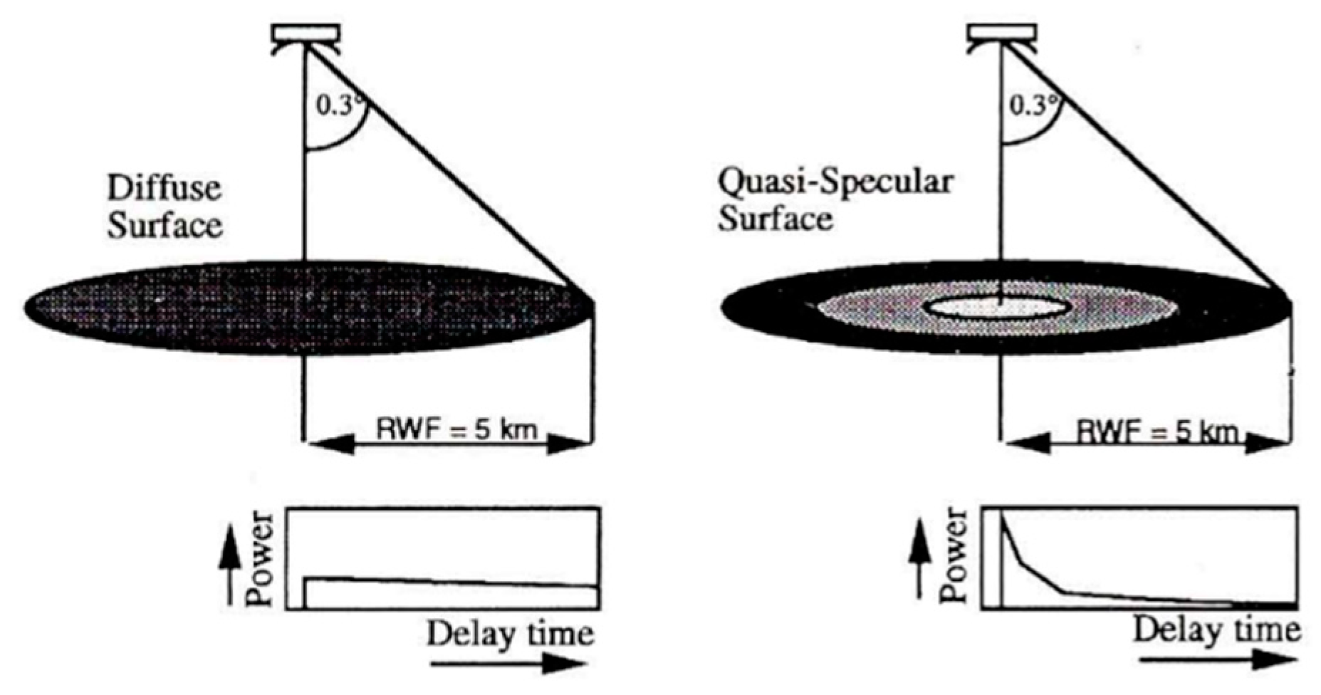
Figure 2.
Spatial coverage of HY-2A/B in the polar regions in November of 2018: (a) Arctic; (b) Antarctic.
Figure 2.
Spatial coverage of HY-2A/B in the polar regions in November of 2018: (a) Arctic; (b) Antarctic.

Figure 3.
Schematic diagram of the Ku Band footprint of the HY-2A/B altimeters.

Figure 4.
Typical waveforms and distribution of the waveforms: (A) Distribution maps of the data, in which the mosaic product of the Sentinel-1a/b (3-day) of the base map shows clear distinctions between the sea ice and seawater; (B) normalized typical waveforms (C1 to C4), in which the original waveforms of the different bands along the orbit are distinguishable.
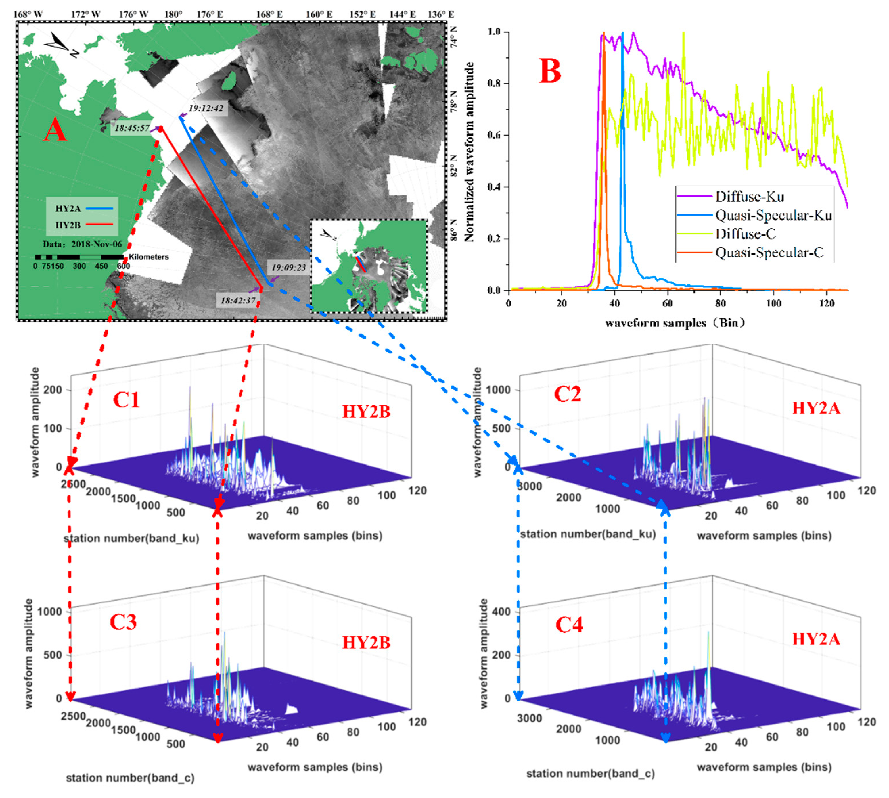
Figure 5.
Waveforms of the SMLE and OCOG from the quasi-specular surfaces: (a) original waveforms of the two different tracking packets; (b) the normalized waveform of the two different tracking packets.
Figure 5.
Waveforms of the SMLE and OCOG from the quasi-specular surfaces: (a) original waveforms of the two different tracking packets; (b) the normalized waveform of the two different tracking packets.

Figure 6.
Original and normalized waveforms of the Suboptimal Maximum Likelihood Estimation (SMLE) and Offset Center of Gravity (OCOG) of the diffuse surfaces.
Figure 6.
Original and normalized waveforms of the Suboptimal Maximum Likelihood Estimation (SMLE) and Offset Center of Gravity (OCOG) of the diffuse surfaces.
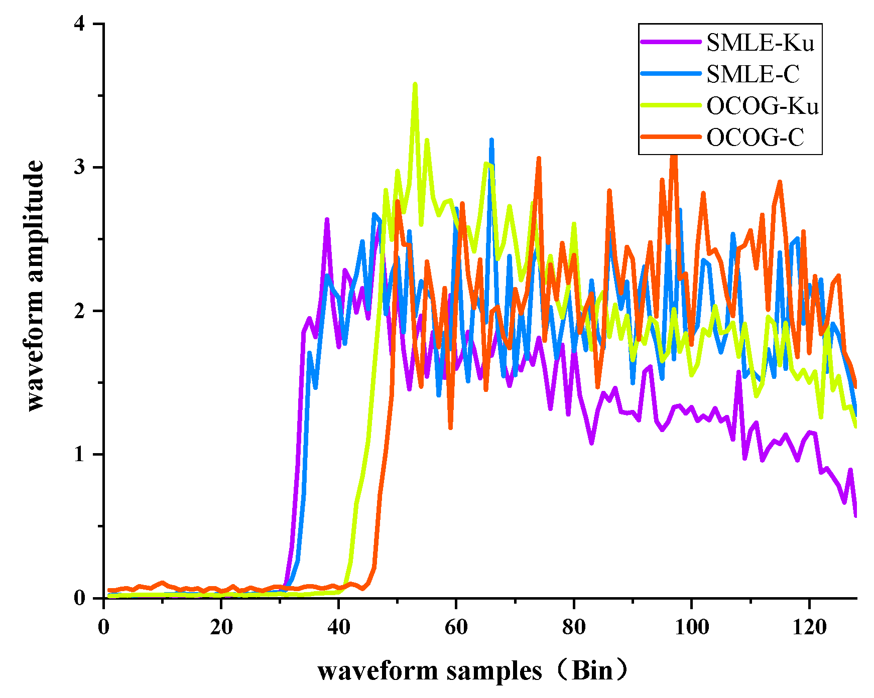
Figure 7.
Cumulative probability distributions for the four cases (seawater, young ice, old ice, and ambiguous ice) for the four waveform parameters: AGC of the C Band; AGC of the Ku Band; PP of the C band; PP of the Ku band. Note: A–D are the results of the HY-2A; E–H are the results of the HY-2B.
Figure 7.
Cumulative probability distributions for the four cases (seawater, young ice, old ice, and ambiguous ice) for the four waveform parameters: AGC of the C Band; AGC of the Ku Band; PP of the C band; PP of the Ku band. Note: A–D are the results of the HY-2A; E–H are the results of the HY-2B.

Figure 8.
Histogram of the sea ice and seawater from the HY-2A/B. Note: A–D are the results of the HY-2A; E–H are the results of the HY-2B.
Figure 8.
Histogram of the sea ice and seawater from the HY-2A/B. Note: A–D are the results of the HY-2A; E–H are the results of the HY-2B.
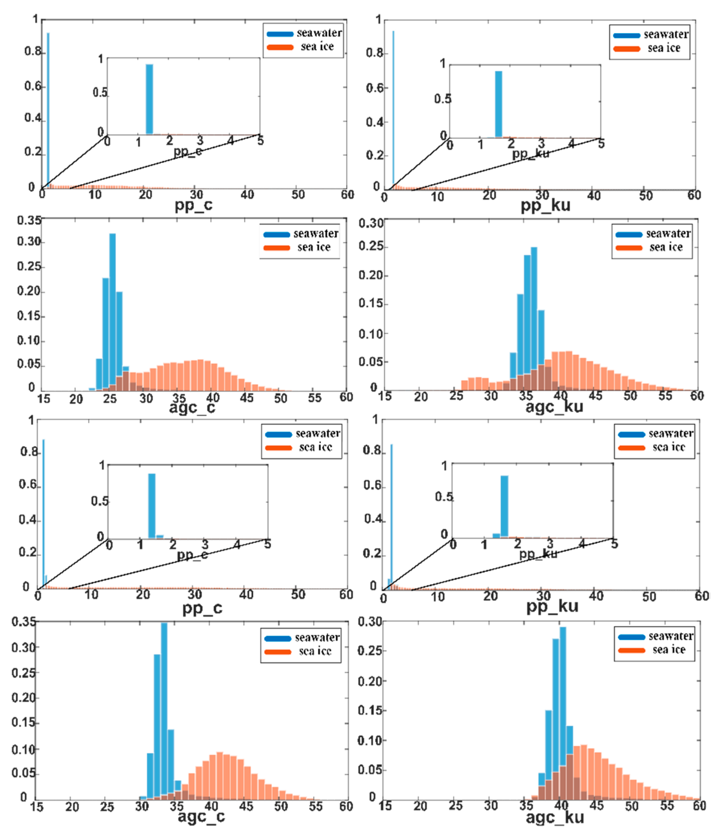
Figure 9.
Cumulative probability distributions for the four cases (open ice, young ice, old ice, and ambiguous ice) for the four waveform parameters: AGC of the C Band; AGC of the Ku Band; PP of the C Band; PP of the Ku Band. Note: A–D are the results of the HY-2A; E–H are the results of the HY-2B.
Figure 9.
Cumulative probability distributions for the four cases (open ice, young ice, old ice, and ambiguous ice) for the four waveform parameters: AGC of the C Band; AGC of the Ku Band; PP of the C Band; PP of the Ku Band. Note: A–D are the results of the HY-2A; E–H are the results of the HY-2B.

Figure 10.
Distributions of classified PP values of the HY-2A ALT data. Note: A1–A4 indicate the Ku Band; B1–B4 indicate the C Band.
Figure 10.
Distributions of classified PP values of the HY-2A ALT data. Note: A1–A4 indicate the Ku Band; B1–B4 indicate the C Band.

Figure 11.
Distributions of the classifications of the PP values of the HY-2B ALT data. Note: A1–A4 indicate the Ku Band; B1–B4 indicate the C Band.
Figure 11.
Distributions of the classifications of the PP values of the HY-2B ALT data. Note: A1–A4 indicate the Ku Band; B1–B4 indicate the C Band.
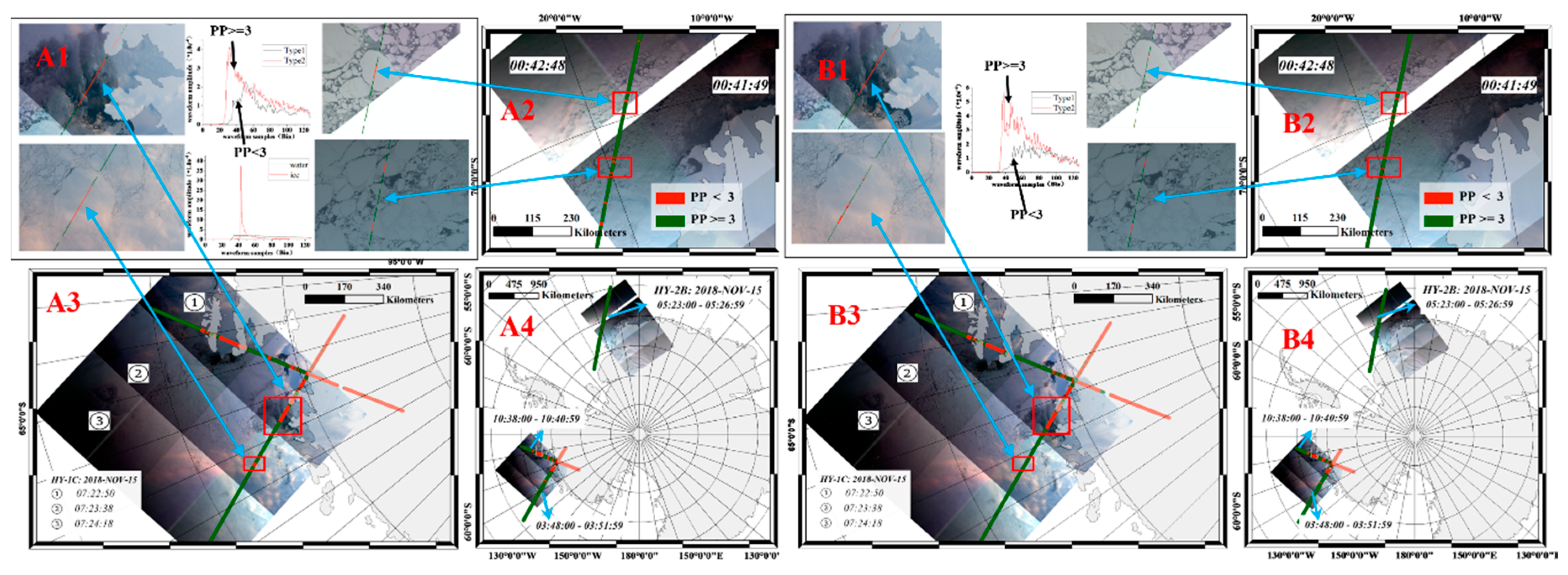
Figure 12.
Distributions of the classifications of the HY-2A/B: A. Distributions of the classifications of the Ku Band’s PP values of HY-2B ALT data; B. distributions of the classifications of the C Band’s PP values of the HY-2B ALT data; C. AARI ice chart; D and E. enlarged drawings of zone 1 (old ice); F and G. enlarged drawings of zone 2 (nilas). Note: in Figure 12A,B, the same colors used in Figure 12C were used to indicate the edges of different ice types.
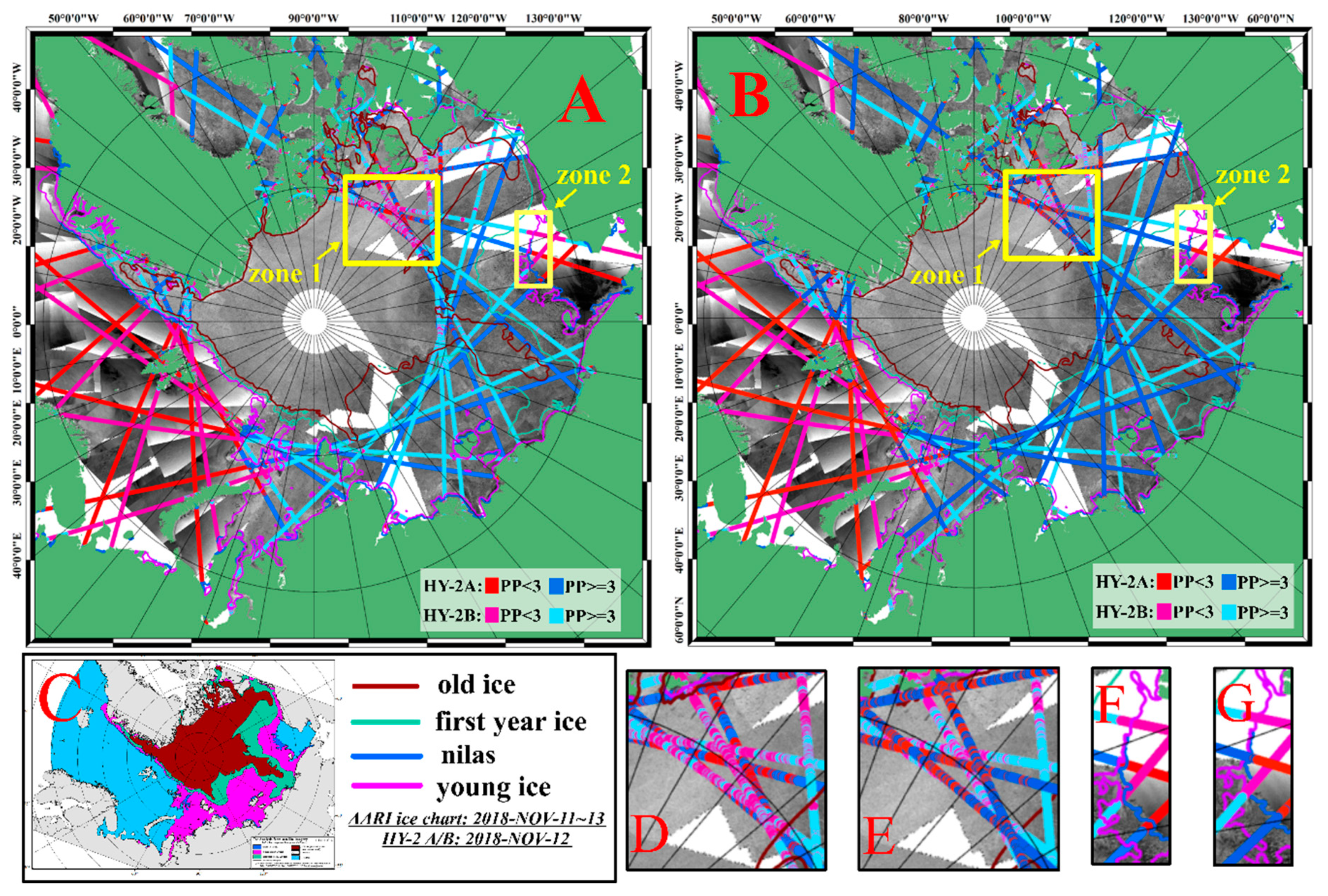
Figure 13.
Average waveforms of the old ice with PP values less than 3 and the average waveforms of the seawater: (a) Average waveform of the Ku Band; (b) average waveform of the C Band. Note: Type 1 waveform was the echoes from the diffuse surfaces of the old ice; Type 2 waveform was the echoes from the diffuse surfaces of the seawater.
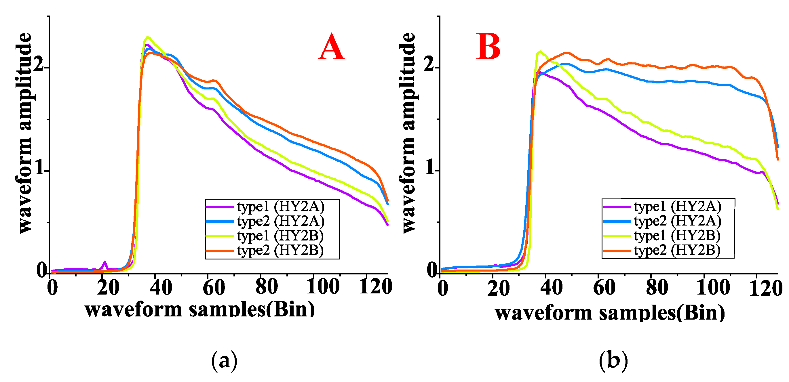
Figure 14.
Histogram of the trailing edge slopes.

Figure 15.
Scatter plots of the Automatic Gain Control (AGC) and Pulse Peaking (PP) values: Figure 15A–D used the data of the HY-2A ALT; Figure 15E–H used the data of the HY-2B ALT; Figure 15A,B,E,F are the scatter plots of the Arctic regions; Figure 15C,D,G,H are the scatter plots of the Antarctic regions.
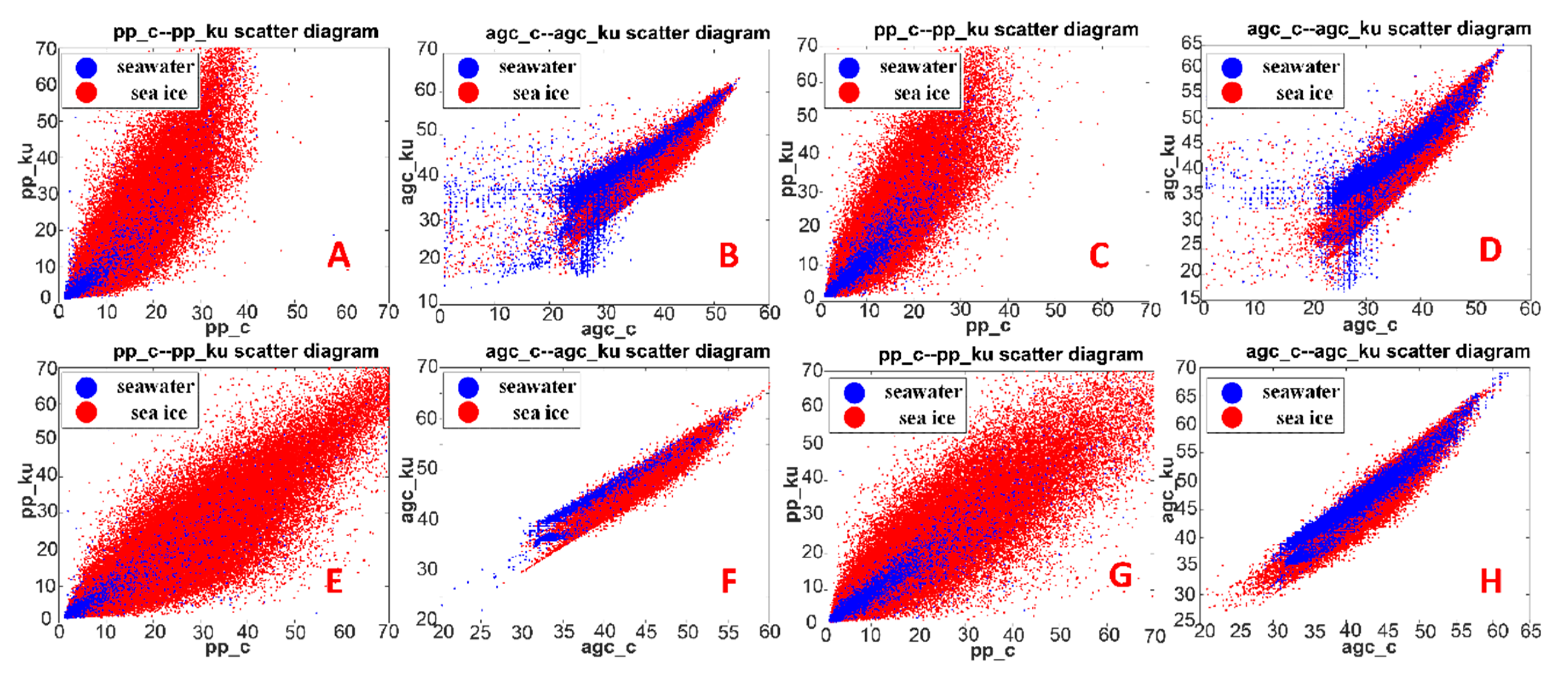
Figure 16.
Daily classification accuracy (November): Figure 16A,B used the data in the Arctic regions; Figure 16C,D used the data in the Antarctic regions; The data of Band Ku were used in Figure 16A,C; The data of Band C were used in Figure 16B,D.

Figure 17.
Classification accuracy rates of the different K values: Figure 17A,B used the data in the Arctic regions; Figure 17C,D used the data in the Antarctic regions; The data of Band Ku were used in Figure 17A,C; The data of Band C were used in Figure 17B,D.

Figure 18.
Distributions of the classification errors of the three methods in the Arctic regions: Figure 18A,E,I and C, G, K indicate the C Band results of the HY-2A/B, respectively; Figure 18B,F,J and D, H, L indicate the Ku Band results of the HY-2A/B, respectively. Note: The color boundaries of the different types of ice in the Figure 18A–L are consistent with the classifications in the ice chart.

Figure 19.
Distributions of the classification errors of the three methods in the Antarctic region: Figure 19A,E,I and C, G, K indicate the C Band results of the HY-2A/B, respectively; Figure 19B,F,J and D, H, L indicate the Ku Band results of the HY-2A/B, respectively. Note: The color boundaries of the different types ice in the Figure 19A–L are consistent with the classifications in the ice chart.

Figure 20.
Sea ice floes of the Antarctic region on 15 November 2018: Figure 20A is the Weddell Sea; Figure 20B is the Pulitzer sea; and Figure 20C is the Ross Sea.

Table 1.
Altimeter parameters (Source: http://www.nsoas.org.cn/).
Table 1.
Altimeter parameters (Source: http://www.nsoas.org.cn/).
| Items | Values | |
|---|---|---|
| Emission signal center frequencies | 13.58 GHz | 5.25 GHz |
| Bandwidth | 102.4 us | |
| AGC dynamic range | 60 dB | |
| Fast Fourier Transform bin number | 128 | |
| Transmitter peak power | ≥10 w | ≥20 w |
| Chirp signal band width | Ku: 320/80/20 MHz (three bandwidths for adaptive adjustments) | |
| C: 160/40/10 MHz (three bandwidths for adaptive adjustments) | ||
Table 2.
Threshold segmentation.
| Type | PP (Ku/C) |
|---|---|
| Ice | <3 |
| Water | > = 3 |
Table 3.
Average classification accuracy.
| Satellite | Band | Sea Ice | Seawater | |
|---|---|---|---|---|
| Arctic | HY2A | C | 89.86% | 96.22% |
| Ku | 88.28% | 96.32% | ||
| HY2B | C | 92.33% | 97.85% | |
| Ku | 88.89% | 98.37% | ||
| Antarctic | HY2A | C | 86.55% | 96.27% |
| Ku | 88.66% | 96.49% | ||
| HY2B | C | 87.93% | 96.09% | |
| Ku | 88.42% | 95.85% |
Table 4.
Average classification accuracy rates.
| Satellite | Band | Sea Ice | Seawater | |
|---|---|---|---|---|
| Arctic | HY2A | C | 87.66% | 95.39% |
| Ku | 85.76% | 98.36% | ||
| HY2B | C | 92.54% | 98.01% | |
| Ku | 87.81% | 97.32% | ||
| Antarctic | HY2A | C | 94.01% | 14.36% |
| Ku | 82.52% | 37.71% | ||
| HY2B | C | 79.78% | 15.57% | |
| Ku | 92.94% | 91.98% |
© 2019 by the authors. Licensee MDPI, Basel, Switzerland. This article is an open access article distributed under the terms and conditions of the Creative Commons Attribution (CC BY) license (http://creativecommons.org/licenses/by/4.0/).
Share and Cite
MDPI and ACS Style
Jiang, C.; Lin, M.; Wei, H. A Study of the Technology Used to Distinguish Sea Ice and Seawater on the Haiyang-2A/B (HY-2A/B) Altimeter Data. Remote Sens. 2019, 11, 1490. https://doi.org/10.3390/rs11121490
AMA Style
Jiang C, Lin M, Wei H. A Study of the Technology Used to Distinguish Sea Ice and Seawater on the Haiyang-2A/B (HY-2A/B) Altimeter Data. Remote Sensing. 2019; 11(12):1490. https://doi.org/10.3390/rs11121490
Chicago/Turabian StyleJiang, Chengfei, Mingsen Lin, and Hao Wei. 2019. "A Study of the Technology Used to Distinguish Sea Ice and Seawater on the Haiyang-2A/B (HY-2A/B) Altimeter Data" Remote Sensing 11, no. 12: 1490. https://doi.org/10.3390/rs11121490
Note that from the first issue of 2016, this journal uses article numbers instead of page numbers. See further details here.