Article

Discovery of the Fastest Ice Flow along the Central Flow Line of Austre Lovénbreen, a Poly-thermal Valley Glacier in Svalbard

1
Chinese Antarctic Center of Surveying and Mapping, Wuhan University, 129 Luoyu Road, Wuhan 430079, China
2
Polar Research Institute of China, 451 Jinqiao Road, Shanghai 200136, China
*
Author to whom correspondence should be addressed.
Remote Sens. 2019, 11(12), 1488; https://doi.org/10.3390/rs11121488
Submission received: 28 May 2019 / Revised: 11 June 2019 / Accepted: 12 June 2019 / Published: 24 June 2019

Abstract

:
Ice flow velocity is a sensitive indicator of glacier variations both controlling and representing the delivery of ice and affecting the future stability of ice masses in a warming climate. As one of the poly-thermal glaciers in the high Arctic, Austre Lovénbreen (AL) is on the northwestern coast of Spitsbergen, Svalbard. The ice flow velocity of AL was investigated using in situ global positioning system (GPS) observations over 14 years and numerical modelling with Elmer/Ice. First, the ice flow velocity field of AL along central flow line was presented and the ice flow velocity is approximately 4 m/a. Obvious seasonal changes of ice flow velocity can be found in the middle of the glacier, where the velocity in spring-summer is 47% larger than in autumn–winter in 2016, and the mean annual velocity increased 14% from 2009 until 2016. Second, the numerical simulation was performed considering the poly-thermal character of the glacier, and indicated that there are two peak ice flow regions on the glacier, and not just one peak ice flow region as previously believed. The new peak ice flow zone found by simulation was verified by field work, which also demonstrated that the velocity of the newly identified zone is 8% faster than the previously identified zone. Third, although our field observations showed that the ice flow velocity is slowly increasing recently, the maximum ice flow velocity will soon begin to decrease gradually in the long term according to glacier evolution modelling of AL.

1. Introduction

Global warming may be particularly marked in the Arctic and has a significant impact on the thermal regime, hydrology, dynamics and mass balance of poly-thermal glaciers [1]. Svalbard, which contains numerous poly-thermal glaciers, has been investigated extensively [2,3,4,5,6,7,8,9]. As a typical Svalbard-type poly-thermal glacier, Austre Lovénbreen (AL) is on the northwestern coast of Spitsbergen. AL is also a small land-terminating valley glacier, and has a length of 4 km, and area of 4.48 km2, and an elevation of 50 to 500 m [10]. AL and its adjacent glaciers in Ny-Alesund, such as Kronebreen, Pedersenbreen, Midtre Lovénbreen (ML), and Austre Brøggerbreen, have a long tradition of hydrological, meteorological, geophysical and glaciological research [11,12,13,14,15]. Glaciological investigations of AL, which began in the 1960s, specifically include mass balance [16], topography [10], temperature [17], moraine dynamics [18], and movement [19,20,21]. However, the seasonal variation of the AL ice flow velocity and the fastest ice flow along the central flow line of AL are unclear.
To ascertain how glaciers behave in the present and future, it is necessary to further investigate the ice flow velocity of glaciers, because the long-term evolution of glacier velocities, which control the delivery of ice to warm, low elevation regions, is an important component of the future stability of ice masses in a warming climate [22]. Poly-thermal glaciers are glaciers that have a mixed basal thermal regime, with a warm-based core, and cold-based ice around its snout and margins [1]. This mix of thermal regimes makes the dynamics of poly-thermal glaciers complex especially in Svalbard, because the water content in the temperate layer of a Svalbard-type poly-thermal glaciers is higher than the typical water content of temperate glaciers [23]. Peak surface velocities were observed shortly after the onset of the melt during summer for many poly-thermal glaciers with in-situ global positioning system (GPS) observations [22,24,25], in-situ total station observations [1] or interferometic synthetic aperture radar (InSAR) [26]. Among the methods in deriving velocities of glaciers, in-situ stakes observations can provide the most accurate coordinates at measuring points for a small region. In contrast, InSAR [27,28,29] and optical imagery [30] can mainly provide information on a large scale [26]. In Svalbard, more than 2100 glaciers cover 36,591 square kilometers, which means most of the glaciers in Svalbard are small, and in situ measurements are more accurate in monitoring the ice flow velocity of such glaciers. In addition, numerical simulation is an essential and powerful tool in predicting the response of glaciers to future climate warming [13]. As the glaciological extension of Elmer, Elmer/Ice is a parallel finite-element model that was originally developed to solve local ice flow problems of high mechanical and physical complexity [31,32], and then updated for applications in ice sheet and ice shelf research [13,33].
In this paper, the ice flow velocity field along the central flow line of AL was obtained accurately by using satellite positioning techniques with in situ observations of AL over 14 years., Numerical simulation was performed to predict the evolution of the ice flow velocity field in the future. Seasonal variations of ice flow velocity, peak ice flow zone and the evolution of ice flow velocity are emphasized in this study. The new findings can deepen the current understanding of ice flow variations and glacier evolution.

2. Data and Methods

The measured surface ice flow velocity of AL was calculated from repeated measurements of stakes by static differential GPS (DGPS) [21,30]. The surface digital elevation model (DEM) of AL was derived from real time kinematics (RTK) [12], and the bedrock DEM of AL was derived from the surface DEM and the ice thickness data was acquired by ground-penetrating radar (GPR) [34]. With surface DEM, bedrock DEM and the measured ice flow velocity field, numerical simulation of the glacier was implemented with Elmer/Ice, and the evolution of the ice flow velocity field was obtained. All these methods are described in the following subsections.

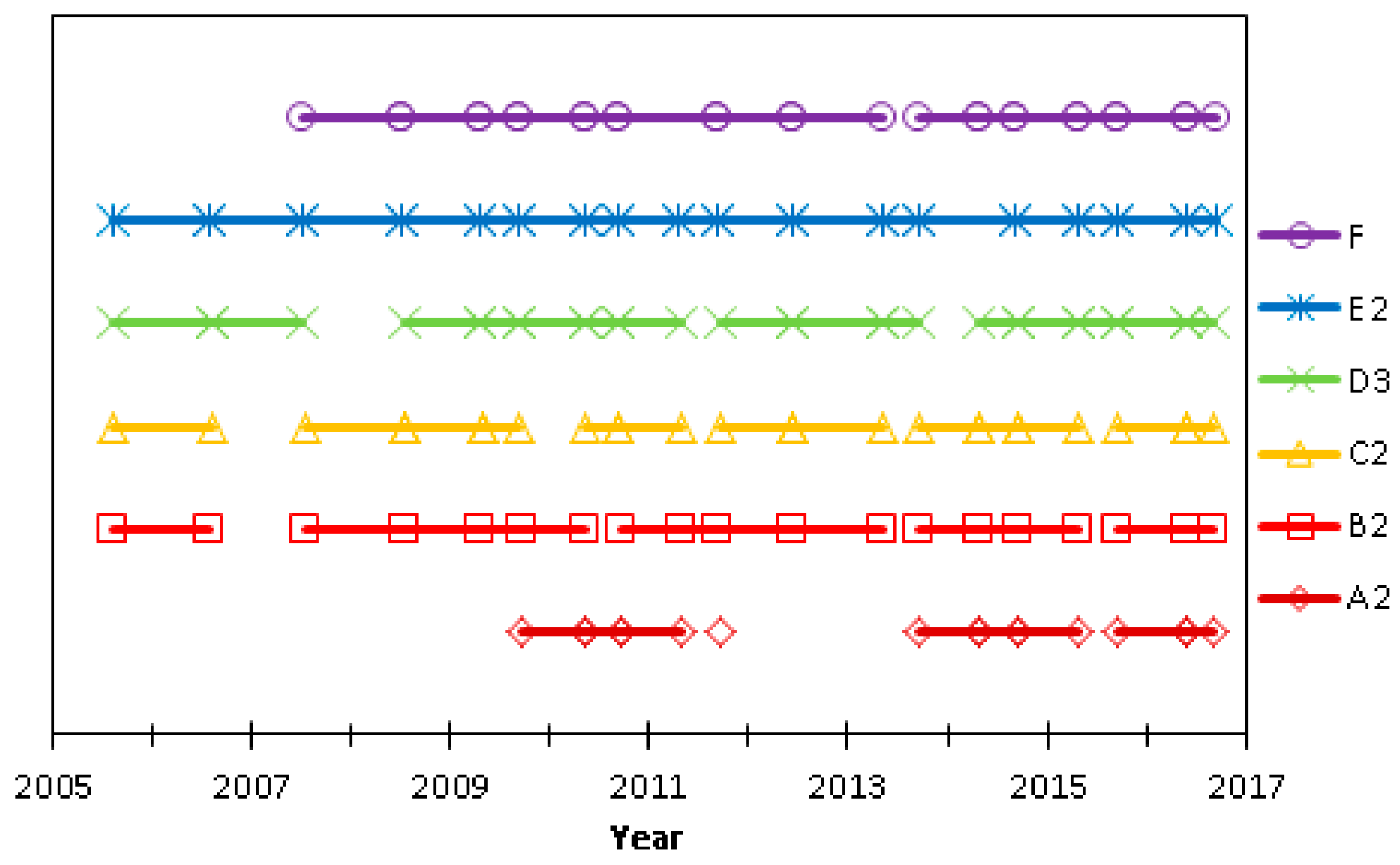
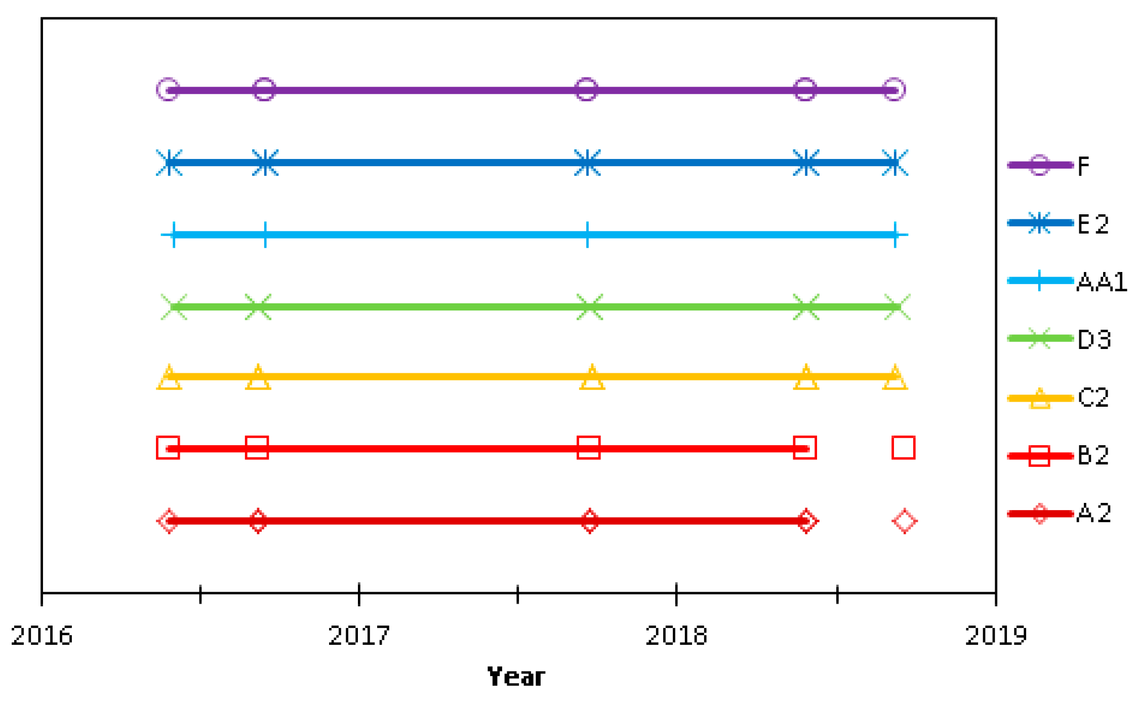
2.1. Stakes Measurement with Static DGPS

Our field work on AL commenced in August 2005, with 16 monitoring stakes on the surface of AL, namely, A1, A2, A3, B1, B2, B3, C1, C2, C3, D1, D2, D3, D4, D5, E1, E2. It is worth noting that stakes A2, B2, C2, D3 and E2 were deployed along the central line of AL that this study determined as the central flow line of AL. During July 2007, an additional stake, called point F, was established upstream of AL to better cover the central flow line. During May 2016, two more stakes, AA1 and AA2, were established in between D3 and E2 to monitor the potential region of the fastest ice flow. At that date, there were 19 stakes on AL, as shown in Figure 1. The stakes were initially made of glass fiber and were updated to aluminum alloy in 2016.
The initial field work stake network design was based on a historical topographic map of the A7 area, Kongsfjorden, Svalbard, which was published by the Norwegian Polar Research Institute (NPI) in 1990 [35]. This map contains ice topographic contours at the scale of 1:100,000 with 25-meter intervals and was generated by aerial surveys. Generally, five to ten stakes are suitable for taking measurements on a small alpine glacier (< 10 km2) [36]. As of 2007, 17 stakes on AL should be sufficient to cover the whole glacier. As shown in Figure 1, which includes the distribution of these stakes and surface topography, stakes A2, B2, C2, D3, E2 and F are located on the central flow line of the glacier representing the maximum flow velocity for the profile. For better coverage of the central flow line, these six stakes were placed at altitude intervals of approximately 60 m, and the altitudes of these stakes, obtained by GPS observations, are shown in Table 1.
The time periods over which the stakes along the central flow line collected observations are shown in Figure 2. Before 2009, field work was carried out in the middle of the year in July or August. Since 2009, the authors have performed field work twice per year, in late April and early September, to better differentiate the variation in AL between winter and summer. Due to the ablation of surface ice, some of the stakes occasionally fell or went missing, and consecutive observations for the same stake were not available. The loss of ice flow data was especially common at point A2.
Static dual-frequency observations at these stakes were obtained from Leica GX1230 and Leica GS10 dual-frequency GPS receivers, and then were calculated in a post-processing procedure by static DGPS with a permanent GPS tracking station in the Chinese Arctic Yellow River Station, which was constructed in 2004 and is 10 km away from the glacier. Highly precise coordinates of the GPS tracking station can be acquired from long-term observations. With static GPS relative positioning by differential dual-frequency GPS observations between the glacier and Yellow River Base, the precise coordinates of these stakes can be obtained at a resolution better than 1 centimeter. To ensure high precision, the observation duration at each stake must not be less than 40 minutes. In addition, the focus was primarily on horizontal velocity, because it is the main factor of controlling the delivery of ice. In contrast, vertical velocity of stakes is far less than horizontal velocity on AL, and is complicated due to ice ablation, ice accumulation, vertical movement of the glacier and vertical variation caused by horizontal movement of stakes [21]. Therefore, this is not discussed in this study.

2.2. DEMs with RTK and GPR

Field works using RTK and GPR were carried out on the glacier at the same time in April of 2009 by a snowmobile carrying measuring instruments. With a Leica GS10 RTK set, kinematic GPS surveying provided the topography of AL over the entire glacier surface in centimeter-level accuracy. The surface DEM with a 10 m grid size is acquired from RTK measurements by kriging interpolation. Ground-based radio-echo sounding revealed the internal structure of the glacier, by using pulseEKKO PRO GPR unit with a 100 MHz antenna set. It is noted that 100 MHz radar is not able to receive continuously a clear reflection signal in the deepest area of the glacier, probably due to existence of temperate ice [34]. Therefore, a homemade 5 MHz radar was used to fill in data gaps by virtue of better penetrability of lower frequency [12]. With analysis of crossing profiles, most depth difference values lie in a Gaussian distribution with a standard deviation of 4.6 m, and are in good agreement with the results of [34,37], in which the bedrock topography uncertainty is 2.6 m over the measurement points. The positioning of GPR profiles was obtained from single point positioning (SPP) by using a single-frequency Leica Smart-VI GPS unit, which is connected to the control unit of GPR. The standard deviation of SPP is approximately 0.3 m, which shows the internal consistency of the GPS survey, and the accuracy of external coincidence is within 0.8m, compared with the accurate coordinates of stakes on the glacier. Finally, a 10 m grid map of bedrock contour of the glacier was easily obtained by subtracting the thickness data from the GPS-derived surface topography.

2.3. Simulation with Elmer/Ice

With the surface DEM, bedrock DEM and measured ice flow velocity field, numerical simulation of the glacier was implemented with Elmer/Ice, and the simulated ice flow velocity field was obtained. In situ observations were helpful for both the modelling and verification of the glacier properties.
The simulation strategy was composed of two steps, a steady-state simulation and dynamic simulation. A finite element grid was constructed first, by dividing the glacier into irregular triangles with the side of 50 m horizontally and into 15 ice layers vertically, in which irregular triangles fit better in tough terrain. The basal friction coefficient and Glen enhancement factor in the ice flow model, β and E, were acquired by a comparison between the measured ice flow velocities from GPS and values from simulations. As early GPS observations showed that C2 was the point with the maximum velocity, the measured velocity at C2 was selected as a control quantity to estimate the parameters mentioned above. The best combination, which had the smallest standard deviation, was treated as the optimal solution for model parameters. Given the poly-thermal nature of the glacier, simulation was performed in three basal conditions, which are no sliding, full sliding and partial sliding. This study found that a sliding phenomenon is expected at the base of all stakes except A1, where the ice thickness was ~20 m. Therefore, in this study, when the ice thickness is greater than or equal to 20 m, the model parameters of the Elmer/Ice model are set as E = 0.865 and β = 0.05, and when the ice thickness is less than 20 m, β = ∞. In consideration of the assumptions and simplifications in the model, a backtracking simulation, by using the historical meteorological records glacier terrain from 1962 to 2009, was performed to verify the modelling results with the measured values and showed that the biases of area, volume and ice thickness in 2009 were 3%, 14% and 11.5%, respectively.
A numerical prediction of AL was carried out under three hypothetical climate scenarios with temperature change rates of 2.2, 4.7, 8.3 °C/100a, in reference to the publication of [38] in which the temperature of the Arctic region will increase by 2.2 °C, 4.2 °C, 5.2 °C, and 8.3 °C under RCP2.6, RCP4.5, RCP6.0, and RCP8.5, respectively. A mean increase of 4.7 °C from the intermediate scenarios, RCP4.5 and RCP6.0, was selected as the most likely temperature change rate for high-probability scenarios, and 2.2 and 8.3 °C were regarded as the lower limit and upper limit of temperature change rate for the pessimistic scenario and optimistic scenario.

3. Results

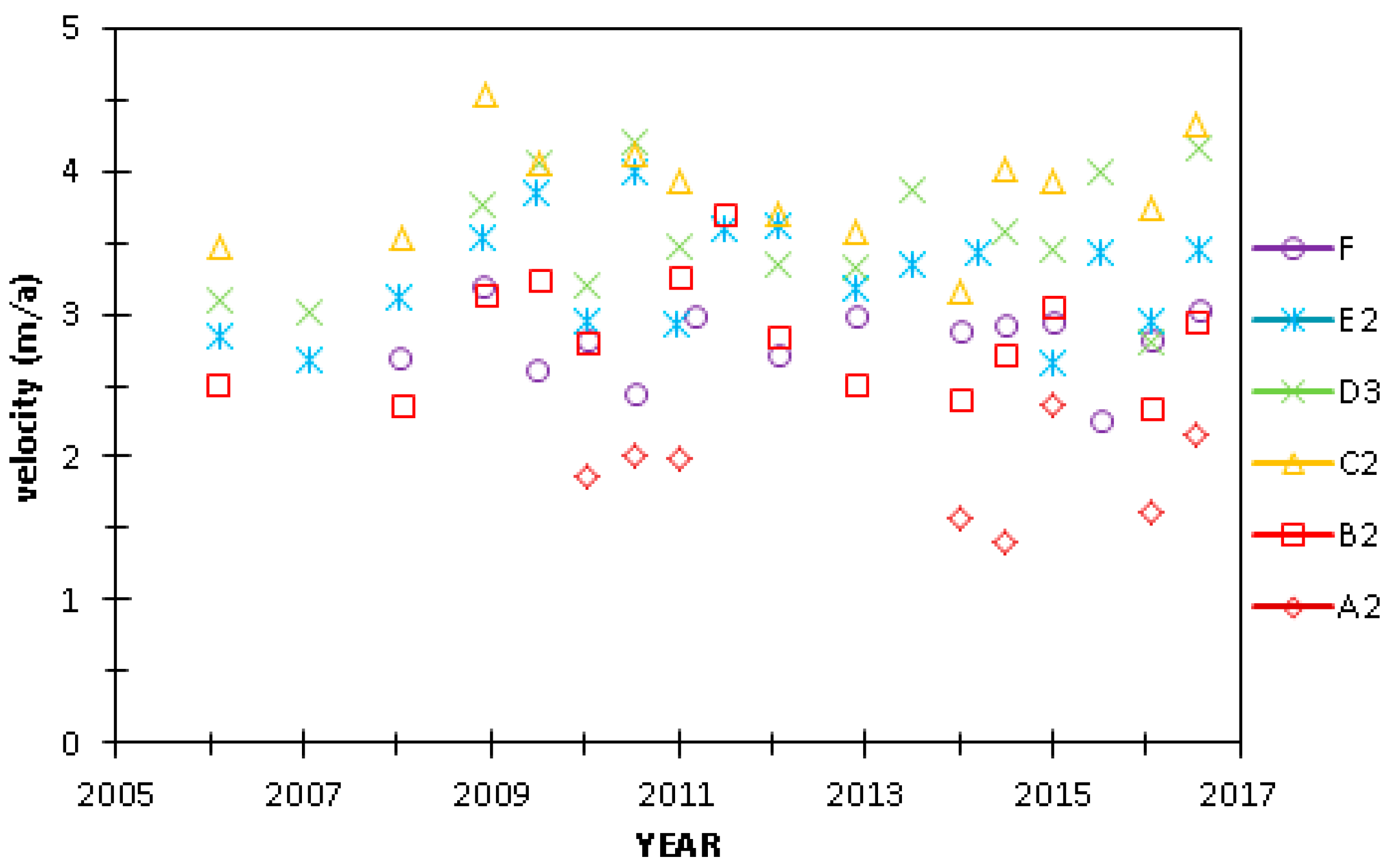
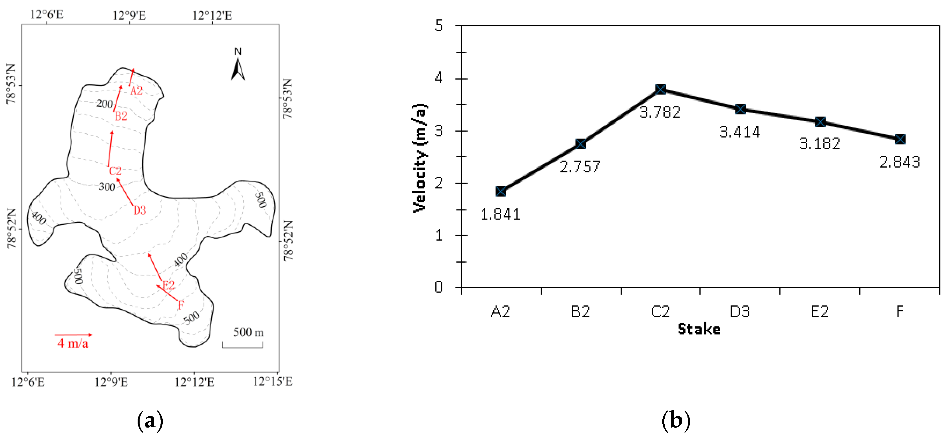
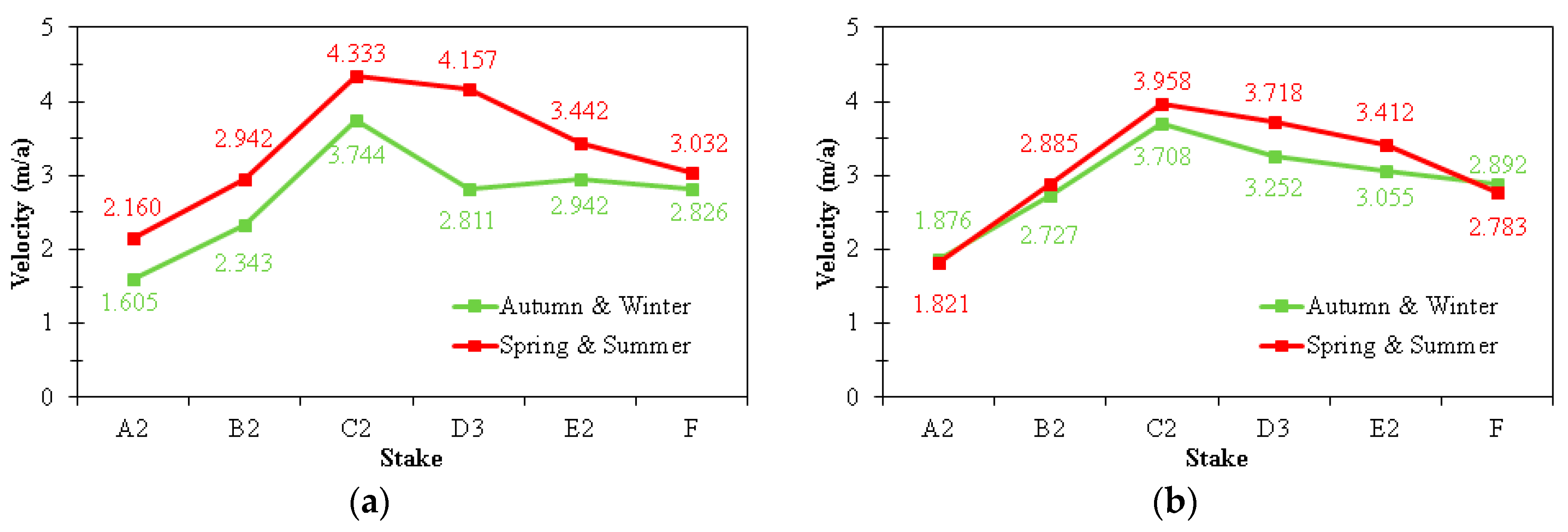
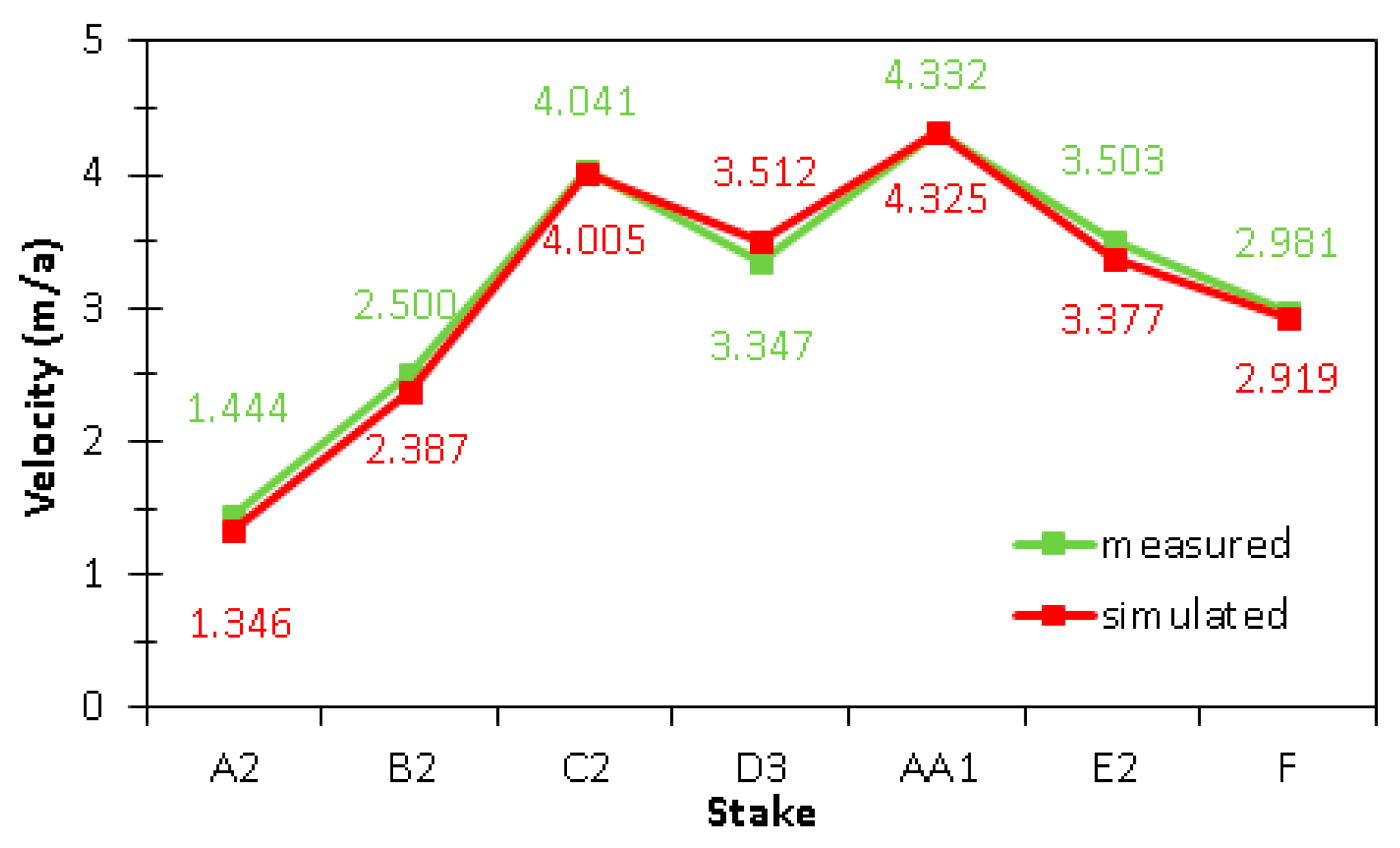
3.1. Measured Ice Flow Velocity

Figure 3 presents the measured velocities for every observation span at the 6 stakes from 2005 to 2016, where each dot represents the mean velocity between two measurements. The ice flow velocity of AL is approximately 4 m/a, and the annual velocity fluctuation of any stake over 12 years can roughly be found. The velocity difference between different stakes and between different seasons are further analyzed in Figure 4 and Figure 5.
It should be noted that the accuracy of velocities can be guaranteed by a precise stake position which is at the level of 1 cm. According to the Gauss normal distribution, 3 times the maximum mean error is taken as a credible measurement error. In the work of [39,40], only single-frequency GPS receivers were used and the horizontal accuracy of each position was estimated to be 1.6 m. For the fastest-moving glaciers, meter-level accuracy is sufficient relative to the annual velocity which is approximately 400 m/a, as the ratio of the 3 time measurement error to the annual movement distance is 1%. For AL, the accuracy of each stake can be better than 1 cm, because dual-frequency GPS receivers were used and then were calculated in a post-processing procedure by static DGPS with a permanent GPS tracking station. Although the annual velocity of AL is just approximately 4 m/a, the ratio of the 3 times measurement error to the annual movement distance is also approximately 1%.
Figure 4 shows the mean velocities from 2005 until 2016 of the stakes, which were obtained by analyzing the time series of the velocities in Figure 3. It should be noted that although annual fluctuations are included in the mean velocities, the velocity difference among stakes can be better illustrated in Figure 4. As shown in Figure 3 and Figure 4, AL moved slowly, with the highest velocity of 3.782 m/a at point C2 and the lowest velocity of 1.841 m/a at point A2. Figure 4a illustrates the relation between surface topography and peak velocity, and Figure 4b clearly shows a peak ice flow zone of velocity of approximately at point C2, which means the middle position was faster than the front and upstream positions.
Due to the difficulty of field work on AL, the coordinates of the stakes could only be acquired once per year before 2008, as mentioned in Section 2. Beginning in 2009, the field work was carried out in late April and early September to better monitor the variation of ice flow in different seasons. According to the movement features of AL and feasibility of field work, spring-summer was defined as the period from late April to early September, and autumn-winter was defined as the period from early September to late April of the next year. The comparisons of the velocities at the 6 stakes during different seasons, are shown in Figure 5, where Figure 5a presents the seasonal difference only in 2016, while Figure 5b demonstrates the mean seasonal difference from 2009 until 2016. As shown in Figure 2, due to the falling and missing of stakes, consecutive observations for the same stake were not available at all stakes except in 2016.
In Figure 5, the seasonal variations of ice flow can be seen clearly and differed among stakes. For the stakes in the snout and margin of AL, the seasonal difference is relatively small, while for the stakes in the middle of AL, the seasonal difference is more obvious. The largest seasonal difference occurred at point D3. In 2016, the velocity in spring-summer at D3 is 47% larger than in autumn-winter. For the mean velocity from 2009 until 2016, the percentage was still up to 14%. In addition, it is important to note that the real seasonal difference could be larger than that shown in Figure 5, because the spring-summer velocity of AL in Figure 5 are just the mean between April and September. However, for poly-thermal glaciers in Svalbard, the peak velocity generally occurs in summer.
The change ratios in the velocities at these stakes, or trends of velocities, are shown in Table 2. First, the change ratio in ice flow velocity at different stakes can be roughly divided into two categories. For points A2 and F, the ice flow remained almost unchanged; for points B2, C2, D3 and E2, the ice flow sped. Second, the trend of the ice flow velocity in middle regions in spring and summer are significantly greater than in autumn and winter, which means acceleration in spring and summer can account for most of the annual variations of velocities.
In addition, compared to the studies of [20,21], the results in the present paper are more reliable because more observations over 14 years are used and seasonal fluctuations are fully considered.

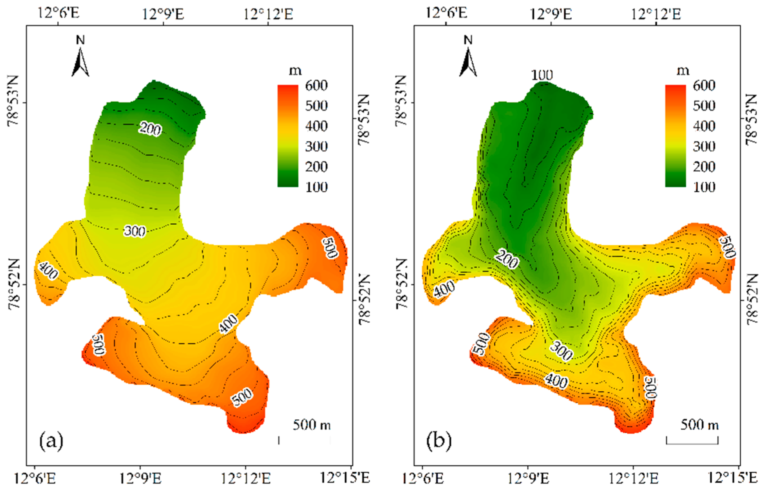
3.2. Surface Contour and Bedrock Contour

Figure 6 presents the surface topography acquired by RTK and bedrock topography provided by subtracting ice thickness data from surface topography. The spatial resolutions of both DEMs are 10 m after kriging interpolation. In Figure 6a, the surface altitude varies from 140 m until 540 m with a gentle incline relative to the length of the glacier. In addition, as shown in the bedrock topography map, bottoms of cross-sections in the front and middle regions of the glacier are concave curves that are perpendicular to the main-stream line, which is a typical characteristic of valley glaciers. The maximum depth in AL is estimated to be 155 m at its central area.

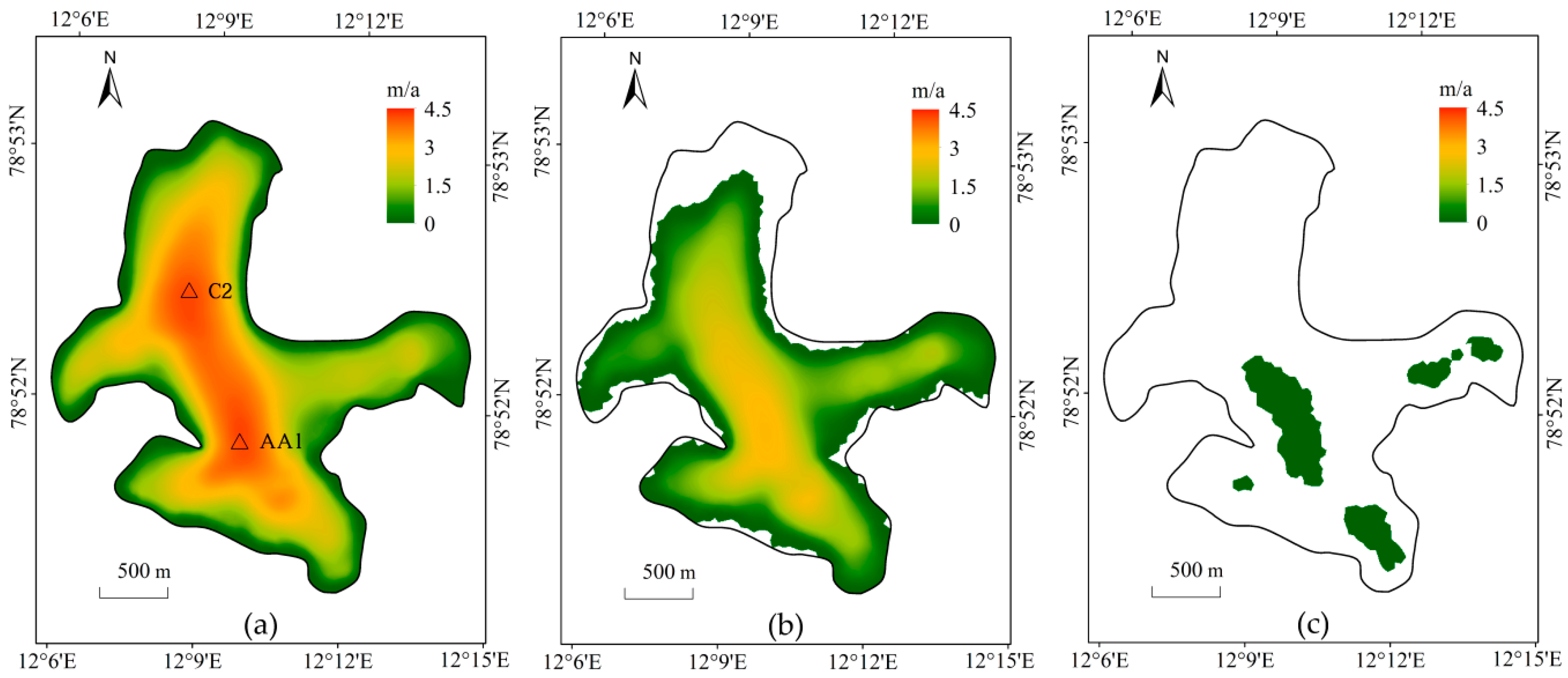
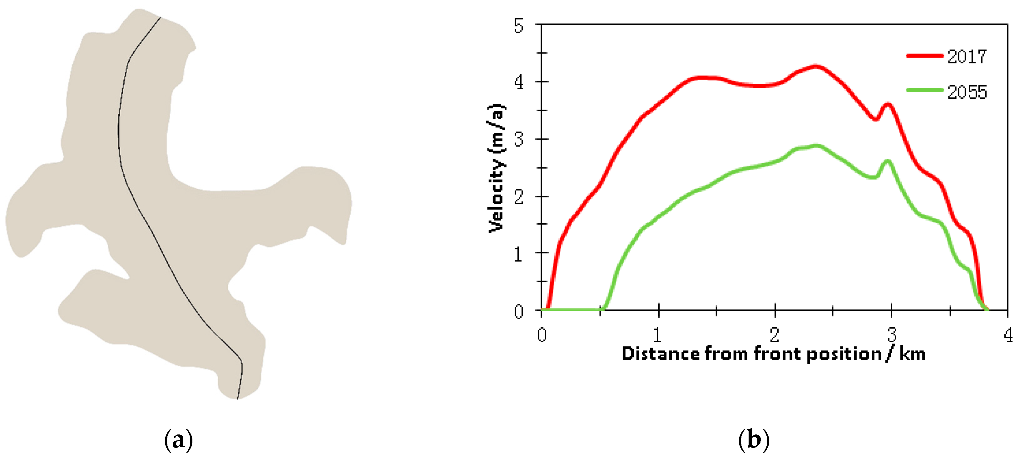
3.3. Discovery of the Fastest Ice Flow
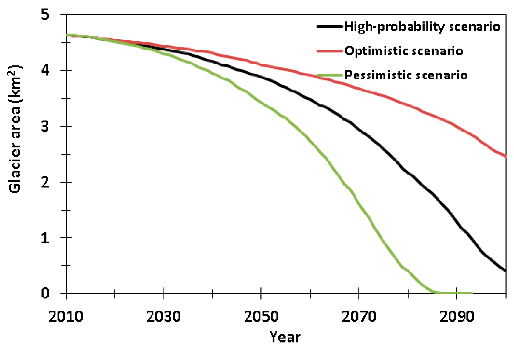
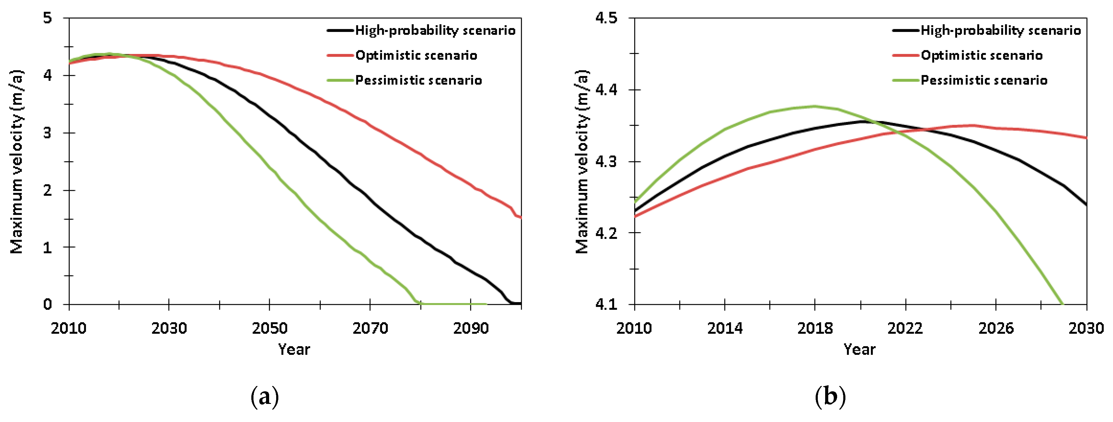
Figure 7 shows the evolution of the ice flow velocity field under the high-probability scenario in 2010, 2055 and 2100. As can be clearly seen in Figure 7a, there are two obvious peak ice flow zones of the ice flow velocity field along the central flow line, named the C2-region and AA1-region. There are also a few peak zones that are too small to be considered. The C2-region decreases rapidly with the shrinkage of the glacier and disappears completely in 2100. The AA1-region is more obvious in Figure 7b,c due to the fast disappearance of the C2-region. The ice flow velocity field in Figure 3, Figure 4 and Figure 5 shows only one maximum velocity zone around point C2, which is different from what is shown in Figure 7. Therefore, this study wanted to determine the number of peak ice flow zones in AL and further, if there are two maximum velocity zones, which zone is the fastest.
In addition, as shown in Figure 7, the surface area of AL significantly declined, which is consistent with the velocity of glacier retreat for 1948–2013 at the mean rate of −16.7 ± 0.3 m/a [10]. For better illustrating the relation between the ice flow velocity field and glacier area, the variations of simulated glacier areas under three hypothetical climate scenarios are given in Figure 8, which shows surface area will decrease sharply in all scenarios. With the rapid shrinkage of the glacier, the ice flow velocity also declines over the entire glacier.
To verify the simulation results, a new stake, named AA1, was established in the potential maximum velocity zone in May 2016. Due to reasons beyond the authors control, field observation missions have not been carried out regularly in the past three years. The entire field work was cancelled in April 2017, and the position of AA1 was not observed in April 2018, and stakes A2 and B2 were not found in September 2018. The actual observation times of 7 stakes along the central flow line are shown in Figure 9.
As shown in Figure 9, the available observations were not taken twice per year over the past three years. Therefore, a comparison between winter and summer could not be conducted, and only the mean measured ice flow velocities during May 2016–September 2018 were compared with simulated velocities, as shown in Figure 10. The modelled velocities coincided well with the measured velocities, and the bias between the simulated and the measured velocities at points AA1 and C2 was less than 1%. Further, the GPS measurements proved that the ice-flow velocity of AA1 was ~8% higher than C2 from May 2016 to September 2018, although the C2 region was thought to be the fastest ice flow area due to the convergence of two tributaries.

4. Discussion

In contrast to Kronebreen, which is the largest glacier in Ny-Alesund and has a mean ice flow velocity of 600 m/a at the glacier front [11], AL moves very slowly. However, compared to Pedersenbreen and ML, which are also valley glaciers and just next to AL, AL has similar ice flow velocities [1,21].
The seasonal change of the ice flow velocity is one of the most essential characteristics for the glaciers in Svalbard. For ML, the short-term velocity variations can be found during July and August [1]. For two calving tidewater glaciers which are near AL, Kronebreen had a distinct seasonal cycle with a minimum speed in autumn and winter, a speedup in spring and a well-pronounced summer peak, while Kongsbreen has relatively stable background velocities during autumn and winter interrupted by a summer speedup during the melt season [39]. For two outlet glaciers of Austfonna, Svalbard, Basin-3 has a prominent summer speedup and Duvebreen has short-lived summer speed-ups between July and September [40]. Therefore, compared to other Svalbard glaciers, AL has a similar seasonal change with speedup during summer, although the specific transition type and transition time are a little different. Given the similarities between ML and AL in location, length, area, elevation and thickness [1], they may have the same movement mechanisms during summer. A temperate ice zone at the glacier bed may enable sliding to occur during summer in response to increased basal water pressure [24]. The possible reason for slight seasonal variation at points A2, B2 and F is that the glacier is poly-thermal with cold ice around its margins where ice is thin. In the studies of [1,22,26,41], daily or weekly velocity variations during summer can be clearly seen from observations. In our study, GPS observations at AL are only available in late April and early September, which means only the mean velocities between April and September can be obtained.
According to studies of [19,20,21] and the preliminary results in Figure 3, Figure 4 and Figure 5 in the present paper, the fastest zone along the central flow line on AL is near point C2, because of the convergence of two tributaries around this region. However, numerical simulation indicated there is a faster region along the central flow line near point AA1, as shown in Figure 7. Field work with a new stake in that region verified the faster region found by simulation, as shown in Figure 4 and Figure 10. The ice flow velocity field along the central flow line of AL shown in Figure 10, can be divided into three regions from upstream to downstream—zones of compression, stretching, and compression. Although C2, D3, AA1, and E2 are all in the stretching zone, the newly found maximum velocity region around point AA1 is faster than stakes C2, D3 and E2. The velocity difference between two peak ice flow regions is likely caused by the bedrock topography and surface morphology of AL as a valley glacier, and the subglacial water due to the thermal regime of AL as a poly-thermal glacier.
As [36] stated, five to ten stakes per glacier are suitable to measure the mass balance of small alpine glaciers (< 10 km2). It seemed reasonable to place 17 stakes on AL in the early field work because AL is less than 5 km2 [10]. However, as shown in the present paper, 17 stakes were not sufficient to obtain the fastest ice flow velocity along the central flow line of AL. This result also indicates that it is necessary to combine field work and numerical simulation data in glacier monitoring to minimize unforeseen errors.
To better understand the evolution of ice flow of AL, the numerical simulation was performed further to discuss the response of the fastest ice flow to future climate warming. Figure 11a denotes the central flow line of AL which is simply derived from central line of AL, and Figure 11b denotes the simulated velocity along the central flow line in 2017 and 2055. In comparison with Figure 10, there are some differences in velocity along the central flow line because the 7 stakes were not located exactly on the midline. However, both figures clearly show a saddle-shaped curve in the middle of AL recently, and the newly found peak ice flow region is slightly larger than the initially identified peak ice flow region. In addition, as shown by the simulated velocity curve in 2055, there will be only one peak ice flow zone along the central flow line near point AA1, which is consistent with the simulated ice flow velocity field in Figure 7.
Figure 12a shows that the maximum ice flow velocity will undergo four stages before its disappearance in 2100: An initial slow increase, a subsequent slow decline, a rapid decline for a long period of time, and a final slow decline. Figure 12b shows that the turning point of the maximum ice flow velocity may occur between 2018–2024 under three hypothetical climate scenarios. Therefore, although our field observations showed that the ice flow velocity field is slowly increasing recently, the maximum ice flow velocity will soon begin to decrease gradually in the long term according to glacier evolution modelling of AL.

5. Conclusions

Ice flow velocity is a key index for glacier variation by controlling the delivery of ice and affecting the future stability of ice masses in a warming climate. To better understand the changes of a typical poly-thermal glacier in the Arctic region, the ice flow velocities along the AL central flow line were investigated using GPS observations and numerical modelling. The fastest ice flow along the central flow line was found with the Elmer/Ice flow model and was verified with in situ GPS measurements. The findings in the present paper can further the understanding of ice flow variations and glacier evolution of AL.
(1) Based on GPS observations from 2005 to 2018, the annual mean velocities of ice flow along the central flow line were obtained, and the seasonal changes in ice flow were differentiated by field work twice per year. The ice flow velocity is approximately 4 m/a and has obvious seasonal differences in the middle of the glacier. The velocity in spring-summer is 47% larger than autumn-winter in 2016, and the mean annual velocity increased 14% from 2009 until 2016.
(2) By considering the poly-thermal character, evolution modelling of the glacier was performed, and the results indicated that there are two regions with maximum ice flow velocity along the central flow line on the glacier, which differs from the previous belief based on early GPS observations that there is only one maximum velocity region. To verify the numerical simulation results, a new stake was established in the newly identified fastest flow zone in 2016, and the in situ measurements demonstrated that the newly found peak ice flow zone was 8% faster than the previously measured peak ice flow zone. This was probably due to their different surface and bedrock environments, such as surface morphology, bedrock topography and subglacial water.
(3) Despite the recent shrinkage of AL, the measured velocity values presented that, in the middle of AL, the ice flow velocity along the central flow line has slowly increased in recent years and numerical simulation also shows that the maximum ice flow velocity will continue to increase over the next several years. However, the maximum ice flow velocity will soon begin to decline over the long-term lifecycle of AL according to glacier evolution modelling of the glacier.

Author Contributions

S.A. and J.A. conceived of the study, supervised the experiments and wrote the manuscript. X.D., G.L. and Z.W. processed some data and produced some of the figures. M.Y. contributed to the field work in the glacier.

Funding

This work was supported by the National Key R&D Program of China (grant number 2016YFC1402701) and the National Natural Science Foundation of China (grant numbers 41531069, 41476162).

Acknowledgments

We greatly appreciate the support from the Chinese Arctic and Antarctic Administration, Ministry of Natural Resources of People’s Republic of China.

Conflicts of Interest

The authors declare no conflicts of interest.

References

  1. Rippin, D.; Willis, I.C.; Arnold, N.; Hodson, A.; Brinkhaus, M. Spatial and temporal variations in surface velocity and basal drag across the tongue of the polythermal glacier midre Lovénbreen, Svalbard. J. Glaciol. 2005, 51, 588–600. [Google Scholar] [CrossRef]
  2. Moholdt, G.; Nuth, C.; Hagen, J.O.; Kohler, J. Recent elevation changes of Svalbard glaciers derived from ICESat laser altimetry. Remote Sens. Environ. 2010, 114, 2756–2767. [Google Scholar] [CrossRef]
  3. James, T.; Murray, T.; Barrand, N.; Sykes, H.; Fox, A.; King, M. Observations of enhanced thinning in the upper reaches of Svalbard glaciers. Cryosphere 2012, 6, 1369–1381. [Google Scholar] [CrossRef] [Green Version]
  4. Małecki, J. Accelerating retreat and high-elevation thinning of glaciers in central Spitsbergen. Cryosphere 2016, 10, 1317–1329. [Google Scholar] [CrossRef] [Green Version]
  5. Førland, E.J.; Benestad, R.; Hanssen-Bauer, I.; Haugen, J.E.; Skaugen, T.E. Temperature and precipitation development at Svalbard 1900–2100. Adv. Meteorol. 2011, 2011. [Google Scholar] [CrossRef]
  6. Hagen, J.O.; Melvold, K.; Pinglot, F.; Dowdeswell, J.A. On the net mass balance of the glaciers and ice caps in Svalbard, Norwegian Arctic. Arct. Antarct. Alp. Res. 2003, 35, 264–270. [Google Scholar] [CrossRef]
  7. Kohler, J.; James, T.; Murray, T.; Nuth, C.; Brandt, O.; Barrand, N.; Aas, H.; Luckman, A. Acceleration in thinning rate on western Svalbard glaciers. Geophys. Res. Lett. 2007, 34. [Google Scholar] [CrossRef] [Green Version]
  8. Nuth, C.; Kohler, J.; König, M.; Deschwanden, A.v.; Hagen, J.O.M.; Kääb, A.; Moholdt, G.; Pettersson, R. Decadal changes from a multi-temporal glacier inventory of Svalbard. Cryosphere 2013, 7, 1603–1621. [Google Scholar] [CrossRef] [Green Version]
  9. Lang, C.; Fettweis, X.; Erpicum, M. Stable climate and surface mass balance in Svalbard over 1979–2013 despite the Arctic warming. Cryosphere 2015, 9, 83–101. [Google Scholar] [CrossRef]
  10. Marlin, C.; Tolle, F.; Griselin, M.; Bernard, E.; Saintenoy, A.; Quenet, M.; Friedt, J.-M. Change in geometry of a high Arctic glacier from 1948 to 2013 (Austre Lovénbreen, Svalbard). Geogr. Ann. Ser. A Phys. Geogr. 2017, 99, 115–138. [Google Scholar] [CrossRef]
  11. Kääb, A.; Lefauconnier, B.; Melvold, K. Flow field of Kronebreen, Svalbard, using repeated Landsat 7 and ASTER data. Ann. Glaciol. 2005, 42, 7–13. [Google Scholar] [CrossRef] [Green Version]
  12. Ai, S.; Wang, Z.; E, D.; Holmen, K.; Tan, Z.; Zhou, C.; Sun, W. Topography, ice thickness and ice volume of the glacier Pedersenbreen in Svalbard, using GPR and GPS. Pol. Res. 2014, 33. [Google Scholar] [CrossRef] [Green Version]
  13. Zwinger, T.; Moore, J. Diagnostic and prognostic simulations with a full Stokes model accounting for superimposed ice of Midtre Lovénbreen, Svalbard. Cryosphere 2009, 3, 217–229. [Google Scholar] [CrossRef]
  14. Tsuji, M.; Uetake, J.; Tanabe, Y. Changes in the fungal community of Austre Brøggerbreen deglaciation area, Ny-Ålesund, Svalbard, High Arctic. Mycoscience 2016, 57, 448–451. [Google Scholar] [CrossRef]
  15. Pramanik, A.; Van Pelt, W.; Kohler, J.; Schuler, T.V. Simulating climatic mass balance, seasonal snow development and associated freshwater runoff in the Kongsfjord basin, Svalbard (1980–2016). J. Glaciol. 2018, 64, 943–956. [Google Scholar] [CrossRef]
  16. Friedt, J.-M.; Tolle, F.; Bernard, E.; Griselin, M.; Laffly, D.; Marlin, C. Assessing the relevance of digital elevation models to evaluate glacier mass balance: Application to Austre Lovénbreen (Spitsbergen, 79 N). Pol. Rec. 2012, 48, 2–10. [Google Scholar] [CrossRef]
  17. Sun, W.; Yan, M.; AI, S.; Zhu, G.; Wang, Z.; Liu, L.; Xu, Y.; Ren, J. Ice Temperature Characteristics of the Austre Lovénbreen Glacier in Ny-Ålesund, Arctic Region. Geomat. Inf. Sci. Wuhan Univ. 2016, 41, 79–85. [Google Scholar] [CrossRef]
  18. Bernard, E.; Friedt, J.-M.; Tolle, F.; Marlin, C.; Griselin, M. Using a small COTS UAV to quantify moraine dynamics induced by climate shift in Arctic environments. Int. J. Remote Sens. 2017, 38, 2480–2494. [Google Scholar] [CrossRef]
  19. Ai, S.; E, D.; Yan, M.; Ren, J. Arctic glacier movement monitoring with GPS method on 2005. Chin. J. Pol. Sci. 2006, 17, 61–68. [Google Scholar]
  20. Xu, M.; Yan, M.; Ren, J.; Ai, S.; Kang, J.; E, D. Surface mass balance and ice flow of the glaciers Austre Lovénbreen and Pedersenbreen, Svalbard, Arctic. Chin. J. Pol. Sci. 2010, 21, 147–159. [Google Scholar]
  21. Ai, S.; Wang, Z.; E, D.; Yan, M. Surface movement research of Arctic glaciers using GPS method. Geomat. Inf. Sci. Wuhan Univ. 2012, 37, 1337–1340. [Google Scholar]
  22. Thomson, L.I.; Copland, L. Changing contribution of peak velocity events to annual velocities following a multi-decadal slowdown at White Glacier. Ann. Glaciol. 2018, 58, 145–154. [Google Scholar] [CrossRef]
  23. Macheret, Y.; Glazovsky, A. Estimation of absolute water content in Spitsbergen glaciers from radar sounding data. Pol. Res. 2000, 19, 205–216. [Google Scholar] [CrossRef]
  24. Bingham, R.G.; Nienow, P.W.; Sharp, M.J. Intra-annual and intra-seasonal flow dynamics of a High Arctic polythermal valley glacier. Ann. Glaciol. 2003, 37, 181–188. [Google Scholar] [CrossRef] [Green Version]
  25. Purdie, H.; Brook, M.; Fuller, I. Seasonal Variation in Ablation and Surface Velocity on a Temperate Maritime Glacier: Fox Glacier, New Zealand. Arct. Antarct. Alp. Res. 2008, 40, 140–147. [Google Scholar] [CrossRef] [Green Version]
  26. Lemos, A.; Shepherd, A.; McMillan, M.E.; Hogg, A. Seasonal Variations in the Flow of Land-Terminating Glaciers in Central-West Greenland Using Sentinel-1 Imagery. Remote Sens. 2018, 10, 1878. [Google Scholar] [CrossRef]
  27. Rabus, B.; Fatland, D.R. Comparison of SAR-interferometric and surveyed velocities on a mountain glacier: Black Rapids Glacier, Alaska, USA. J. Glaciol. 2000, 46, 119–128. [Google Scholar] [CrossRef]
  28. Strozzi, T.; Luckman, A.; Murray, T.; Wegmuller, U.; Werner, C.L. Glacier motion estimation using SAR offset-tracking procedures. IEEE Trans. Geosci. Remote Sens. 2002, 40, 2384–2391. [Google Scholar] [CrossRef] [Green Version]
  29. Quincey, D.J.; Luckman, A.; Benn, D. Quantification of Everest-region glacier velocities between 1992 and 2002, using satellite radar interferometry and feature tracking. J. Glaciol. 2009, 55. [Google Scholar] [CrossRef]
  30. Berthier, E.; Vadon, H.; Baratoux, D.; Arnaud, Y.; Vincent, C.; Feigl, K.L.; Rémy, F.; Legrésy, B. Surface motion of mountain glaciers derived from satellite optical imagery. Remote Sens. Environ. 2005, 95, 14–28. [Google Scholar] [CrossRef]
  31. Le Meur, E.; Gagliardini, O.; Zwinger, T.; Ruokolainen, J. Glacier flow modelling: A comparison of the Shallow Ice Approximation and the full-Stokes solution. C. R. Phys. 2004, 5, 709–722. [Google Scholar] [CrossRef]
  32. Gagliardini, O.; Zwinger, T.; Gillet-Chaulet, F.; Durand, G.; Favier, L.; Fleurian, B.d.; Greve, R.; Malinen, M.; Martín, C.; Råback, P.; et al. Capabilities and performance of Elmer/Ice, a new-generation ice sheet model. Geosci. Model Dev. 2013, 6, 1299–1318. [Google Scholar] [CrossRef] [Green Version]
  33. Zwinger, T.; Greve, R.; Gagliardini, O.; Shiraiwa, T.; Lyly, M. A full Stokes-flow thermo-mechanical model for firn and ice applied to the Gorshkov crater glacier, Kamchatka. Ann. Glaciol. 2007, 45, 29–37. [Google Scholar] [CrossRef] [Green Version]
  34. Saintenoy, A.; Friedt, J.-M.; Booth, A.D.; Tolle, F.; Bernard, E.; Laffly, D.; Marlin, C.; Griselin, M. Deriving ice thickness, glacier volume and bedrock morphology of the Austre Lovénbreen (Svalbard) using Ground-penetrating Radar. Near Surf. Geophys. Eur. Assoc. Geosci. Eng. (EAGE) 2013, 11, 253–261. [Google Scholar] [CrossRef]
  35. Norwegian Polar Institute. Geological Map of Svalbard, Scale 1:100000. Sheet A7, Kongsfjorden; Norwegian Polar Institute: Tromso, Norway, 1990. [Google Scholar]
  36. Fountain, A.G.; Vecchia, A. How many stakes are required to measure the mass balance of a glacier? Geogr. Ann. Ser. A Phys. Geogr. 1999, 81, 563–573. [Google Scholar] [CrossRef]
  37. Bernard, E.; Friedt, J.-M.; Saintenoy, A.; Tolle, F.; Griselin, M.; Marlin, C. Where does a glacier end? GPR measurements to identify the limits between valley slopes and actual glacier body. Application to the Austre Lovénbreen, Spitsbergen. Int. J. Appl. Earth Obs. Geoinf. 2014, 27, 100–108. [Google Scholar] [CrossRef]
  38. Collins, M.; Knutti, R.; Arblaster, J.; Dufresne, J.-L.; Fichefet, T.; Friedlingstein, P.; Gao, X.; Gutowski, W.J.; Johns, T.; Krinner, G.; et al. Long-Term Climate Change: Projections, Commitments and Irreversibility; Intergovernmental Panel on Climate Change (IPCC): Cambridge, UK; New York, NY, USA, 2013. [Google Scholar]
  39. Schellenberger, T.; Dunse, T.; Kääb, A.; Kohler, J.H.; Reijmer, C. Surface speed and frontal ablation of Kronebreen and Kongsbreen, NW Svalbard, from SAR offset tracking. Cryosphere 2015, 9, 2339–2355. [Google Scholar] [CrossRef] [Green Version]
  40. Dunse, T.; Schuler, T.V.; Hagen, J.O.; Reijmer, C.H. Seasonal speed-up of two outlet glaciers of Austfonna, Svalbard, inferred from continuous GPS measurements. Cryosphere 2012, 6. [Google Scholar] [CrossRef]
  41. Köhler, A.; Chapuis, A.; Nuth, C.; Kohler, J.; Weidle, C. Autonomous detection of calving-related seismicity at Kronebreen, Svalbard. Cryosphere 2012, 6, 393–406. [Google Scholar] [CrossRef] [Green Version]
Figure 1. Distribution of 19 stakes on AL. Stakes A1, A2, A3, B1, B2, B3, C1, C2, C3, D1, D2, D3, D4, D5, E1, E2 were built in August 2005. Stake F was built in July 2007. Stakes AA1 and AA2 were built in May 2016.
Remotesensing 11 01488 g001
Figure 2. Available observations of 6 stakes along the central flow line of AL from 2005 to 2016. Different colors denote different stakes. Each mark corresponds to a single measurement time. A line between two points indicates the period over which the velocity can be acquired based on the difference in the coordinates of the two points.
Remotesensing 11 01488 g002
Figure 3. The measured velocities (m/a) for every observation span at the 6 stakes along the central flow line, 2005–2016. The different colors denote different stakes. Each dot corresponds to the mean velocity between two measurements.
Remotesensing 11 01488 g003
Figure 4. The mean velocities (m/a) over 2005-2016 of stakes along the central flow line. (a) The ice flow velocity field along the central flow line. (b) The velocity values at 6 stakes.
Remotesensing 11 01488 g004
Figure 5. (a) The comparison of velocities (m/a) in different seasons in 2016. (b) The comparison of mean velocities (m/a) in different seasons over 2009–2016. The different colors denote different seasons.
Remotesensing 11 01488 g005
Figure 6. (a) Surface topography map of AL. (b) Bedrock topography map of AL. The contour interval is 25 m for both maps.
Remotesensing 11 01488 g006
Figure 7. Simulated ice flow velocity field of AL under the high-probability scenario in 2010 (a), 2055 (b) and 2100 (c).
Remotesensing 11 01488 g007
Figure 8. Simulated glacier areas as a function of time under three hypothetical climate scenarios, 2010~2100.
Remotesensing 11 01488 g008
Figure 9. The available observations for 7 stakes along the central flow line, May 2016–Sep. 2018. Different colors denote different stakes. Each mark corresponds to a specific measurement, and each line between two marks indicates that the velocity during that period could be acquired from the difference between the first and second coordinates at the stakes.
Remotesensing 11 01488 g009
Figure 10. The comparison of the simulated and measured (May 2016-Sep., 2018) velocities (m/a) of 7 stakes along the central flow line. The different colors denote measured or simulated measurements.
Remotesensing 11 01488 g010
Figure 11. (a) The sketch of central flow line of AL. (b) Curves of simulated velocity (m/a) along central flow line in 2017 and 2055.
Remotesensing 11 01488 g011
Figure 12. The simulated maximum ice flow velocity as a function of time under three hypothetical climate scenarios during 2010~2100 (a) and during 2010~2030 (b).
Remotesensing 11 01488 g012
Table 1. Altitudes and measuring time of 6 stakes along the central flow line of AL.
A2B2C2D3E2F
Altitude(m)200.884249.052313.735367.152445.456508.345
Measuring timeAug., 2005Aug., 2005Aug., 2005Aug., 2005Aug., 2005Jul., 2007
Table 2. Trends of velocities at 6 stakes along the central flow line of AL, in different seasons (unit: mm/a2).
A2B2C2D3E2F
Trend annually−9−91030122
Trend in autumn & winter−13−7−11−613−3
Trend in spring & summer−132456843−1

