Joint Local Block Grouping with Noise-Adjusted Principal Component Analysis for Hyperspectral Remote-Sensing Imagery Sparse Unmixing


1
School of Computer Science, China University of Geosciences (Wuhan), Wuhan 430074, China
2
Hubei Key Laboratory of Intelligent Geo-Information Processing, China University of Geosciences, Wuhan 430074, China
3
State Key Laboratory of Information Engineering in Surveying, Mapping, and Remote Sensing, Wuhan University, Wuhan 430079, China
4
Hubei Province Engineering Research Center of Natural Resources Remote Sensing Monitoring, Wuhan 430079, China
*
Author to whom correspondence should be addressed.
Remote Sens. 2019, 11(10), 1223; https://doi.org/10.3390/rs11101223
Submission received: 18 April 2019
/
Revised: 17 May 2019
/
Accepted: 21 May 2019
/
Published: 23 May 2019
(This article belongs to the Special Issue Dimensionality Reduction for Hyperspectral Imagery Analysis)
Abstract
:Spatial regularized sparse unmixing has been proved as an effective spectral unmixing technique, combining spatial information and standard spectral signatures known in advance into the traditional spectral unmixing model in the form of sparse regression. In a spatial regularized sparse unmixing model, spatial consideration acts as an important role and develops from local neighborhood pixels to global structures. However, incorporating spatial relationships will increase the computational complexity, and it is inevitable that some negative influences obtained by inaccurate estimated abundances’ spatial correlations will reduce the accuracy of the algorithms. To obtain a more reliable and efficient spatial regularized sparse unmixing results, a joint local block grouping with noise-adjusted principal component analysis for hyperspectral remote-sensing imagery sparse unmixing is proposed in this paper. In this work, local block grouping is first utilized to gather and classify abundant spatial information in local blocks, and noise-adjusted principal component analysis is used to compress these series of classified local blocks and select the most significant ones. Then the representative spatial correlations are drawn and replace the traditional spatial regularization in the spatial regularized sparse unmixing method. Compared with total variation-based and non-local means-based sparse unmixing algorithms, the proposed approach can yield comparable experimental results with three simulated hyperspectral data cubes and two real hyperspectral remote-sensing images.
1. Introduction
Hyperspectral unmixing has become an alluring research topic with the development of hyperspectral remote sensors [1,2,3]. Mixed pixels are common in remotely sensed hyperspectral images, due to the imaging spectrometer’s insufficient spatial resolution as well as the intimate mixing effects [4,5,6]. Hyperspectral unmixing is a widely used technique to solve the mixed pixel problem according to analyzing the potential materials existing in each pixel and estimating the proportions of different materials [7,8]. Here, the materials in a mixed pixel are called endmembers, and the computed proportions are denoted as fractional abundances. Hence, hyperspectral unmixing is aimed at precisely estimating the endmembers together with the fractional abundances. Usually, there are two main categories of spectral unmixing models, namely, the linear-mixture-based models and the non-linear mixing models. Because of the computational tractability and flexibility in different applications of linear-mixture-based models [9,10,11], in this paper we will focus on the study of linear spectral unmixing.
Traditionally, hyperspectral unmixing is divided into two stages, endmember selection and fractional abundance estimation [12]. In addition, blind source separation (BSS)-based unsupervised unmixing methods [13,14,15,16], such as independent component analysis [13] or non-negative matrix/tensor factorization based hyperspectral unmixing [14,15,16], also have been proven to be able to unmix highly mixed datasets and achieve comparable unmixing accuracy. However, due to the separation of the two stages in traditional spectral unmixing methods, the endmember estimation errors and fractional abundances estimation errors might be accumulated [17], which would lead to poor unmixing results; while the unsupervised unmixing techniques might also fail since they could extract virtual endmembers without any physical meaning, or these methods can only work under the hypothesis that there is pure pixel existing, which is hard to guarantee in reality [18,19,20,21].
More recently, spectral variability, due to illumination conditions, topography, atmospheric effects, or some intrinsic variability of material, has attracted considerable attention in hyperspectral unmixing. The dictionary-adjusted non-convex sparsity-encouraging regression (DANSER) [22] algorithm was proposed as a spectral-library-based spectral unmixing approach, aiming to model the differences between the standard spectral library and the observed spectral signatures, and these differences are treated as spectral variability. Similarly as to modelling the differences, perturbed linear mixing model (PLMM) was introduced with a perturbation term accounting for the endmember variability [23]. Considering the scale differences between endmembers, extended liner mixing model (ELMM) was presented [24]. Later, an augmented linear mixing model (ALMM) to address spectral variability for hyperspectral unmixing [25] was proposed combining the advantages of PLMM and ELMM, together with the novel idea about the spectral variability dictionary, which has led to the state-of-the-art performance. Simultaneously, many other strategies have also been presented to address the spectral variability for spectral unmixing, such as mixed norms [26], low-rank attribute [27]. In this paper, spectral variability is not the point of our discussion, and more attention will be paid to improving the accuracy of the traditional spectral unmixing algorithms.
In recent years, sparse unmixing acted as a semi-supervised spectral unmixing technique has attracted much attention [28,29,30,31], since it can better utilize the standard spectral library, which was collected and built under ideal condition, and circumvent the challenge of endmember selection. Then, the hyperspectral unmixing via sparse representation becomes a combination problem which amounts to determining the best combination of spectral signatures in the spectral library known in advance. Owing to the conflict between the large number of spectral signatures in spectral library and the small number of endmembers existing in each mixed pixel, the sparse constraint is imposed in the classical linear mixture model. The original sparse unmixing model can then be written as,
where denoted as L0 norm, is used to compute the number of non-zero components of vector x, and acts as the error tolerance due to the model error and noise. Here, is one of the pixels in hyperspectral remote sensing images, and is the standard spectral library known in advance. Besides, represents the fractional abundance vector responding to the library A. Given y and A, considering the abundance non-negativity constraint (denoted as ANC, ), the objective of (1) is to compute the fractional abundance values, x. Because the objective function (1) is a typical NP-hard problem(meaning that the problem is combinatorial and very complex to solve) [29,32] and the traditional optimization methods cannot solve it directly. To better tackle the NP-hard problem, usually L1 norm is used to replace the original L0 norm under the certain conditions [33]. With the development of a sparse representation-based spectral unmixing algorithm, more and more sparse unmixing algorithms have been proposed to further enhance the precision of sparse unmixing [34,35,36,37], such as orthogonal matching pursuit (OMP) [34] for spectral unmixing, sparse unmixing via variable splitting and augmented Lagrangian (SUnSAL) [35], the sparse unmixing method based on noise-level estimation (SU-NLE) [36], and the least angle regression-based constrained sparse unmixing (LARCSU) [37].
With the deep research in spectral unmixing, spatial regularization sparse unmixing (SRSU) algorithms have been widely studied [38,39,40,41,42,43,44,45] and proved to be far better than the traditional spectral unmixing methods. Hence, spatial information has been recognized, utilized, and incorporated in the traditional spectral unmixing model as prior knowledge, such as sparse unmixing via variable splitting augmented Lagrangian and total variation (SUnSAL-TV) [38], non-local sparse unmixing (NLSU) [39], and collaborative SUnSAL [40,41]. In these models, spatial correlations has been developed from a local pixel between a pixel and pixels [46,47,48] to a non-local block [49,50] among searching windows, and different spatial information is considered in form of different regularizations, such as neighborhood filters [51], variational forms [52,53,54]. Different methods have their unique performance. For example, the SUnSAL-TV algorithm takes TV regularizer accounting for spatial homogeneity in a first-order pixel neighborhood system. While, adaptive non-local Euclidean medians sparse unmixing (ANLEMSU) method [42] utilizes non-local Euclidean medians filtering approach for spatial consideration replaced the non-local means total variation spatial operator in non-local sparse unmixing (NLSU) algorithm. These non-local series sparse unmixing algorithms have obtained many competitive results except for the negative influences of inaccurate estimated unmixing abundances or called outliers in abundances, and the huge computational pressure, since nonlocal-methods should compute weights averaging of different groups of non-local pixels’ abundance, which is quite time-consuming.
Differing from NLSU, to obtain a more accurate and efficient SRSU results, a joint local block grouping with noise-adjusted principal component analysis method is used to consider spatial information in a sparse unmixing process. The major differences between NLSU and the proposed method is the consideration of the non-local spatial information. In NLSU, every local block in the abundance map is used to estimate the spatial influence to the current pixel’s abundance value, which means all the local blocks are considered and computed along the unmixing process. While, in this paper, local blocks are treated as a series of vector variables, and these variables are selected by grouping the pixels with similar local spatial structures to the underlying one in the local window. This is the first step called local block grouping aiming to collect edge structures or textures of fractional abundance images. Then noise-adjusted principal component analysis (NAPCA) [55,56] is undertaken to transform the original datasets into the principal component analysis (PCA) domain and maintain only the most significant principal component as well as wipe off the inaccurate estimated fractional abundances. PCA acted as a versatile technique has been used widely in image processing for various applications [57], such as dimensionality reduction [58,59], feature extraction [60,61]. NAPCA is an improved algorithm which ranks transformed principal components based on maximization of SNR rather than variance as traditional PCA. Compared with PCA, NAPCA can better address signals with small variances but high qualities. To acquire accurate local spatial information, NAPCA is taken to shrink the local block groups and discard some poor local blocks. Compared with total variation-based and non-local means-based SRSU algorithms, the proposed joint local block grouping with the NAPCA sparse unmixing method can yield competitive results with state-of-the-art spatial sparse unmixing algorithms using three simulated hyperspectral datasets and two real hyperspectral images.
The rest of this paper is structured as follows. Section 2 briefly reviews the fundamental model of SRSU algorithms. Section 3 presents the proposed model, joint local block grouping with NAPCA sparse unmixing method. In Section 4 and Section 5, the experimental results and analysis will be made in both qualitative and quantitative with simulated datasets and real hyperspectral images. Finally, the conclusions are drawn in Section 6.
2. Spatial Regularization Sparse Unmixing (SRSU) Model
Sparse unmixing can better solve the challenging problem of endmember selection with the utilization of a standard spectral library as well as sparse representation optimization method. However, classical sparse unmixing focuses on the analysis of spectral information of hyperspectral remote-sensing image alone, no spatial information has been taken into consideration, although hyperspectral remote-sensing imagery are images primarily. To mitigate the limitation of exploiting the spatial correlation present in hyperspectral remote-sensing imagery, accordingly, spatial information has been studied and used in classical sparse unmixing model, such as the utilization of total variation regularization, nonlocal means regularization, local collaborative considerations.
Owing to the successful application of spatial information, SRSU has achieved better performance and then, SRSU strategy has attracted more and more attention. The general SRSU model can be represented as follows:
where represents the observed hyperspectral dataset containing n pixels with L bands, written in the form of a matrix, and denotes the standard spectral library, in which m is the number of endmembers in A. is the fractional abundance map, corresponding to the input hyperspectral dataset Y as well as standard spectral library A. is the data-fitting term, and denotes the Frobenius norm. , and denotes the j-th column of X. The last term, , is used for considering the physical constraint obeying the basic ground distribution reality, abundance non-negativity constraint, written as ANC.
Jspt(X) is a general expression used for the consideration of spatial information. Different consideration of the spatial information leads to different spatial smoothness terms Jspt(X). For example, a TV-based SRSU model is written as:
where TV is induced as spatial regularization and aimed at promoting piecewise smooth transitions of abundance images X. This spatial regularizer accounts for spatial homogeneity of fractional abundance images, assuming that two neighboring pixels would have similar fractional abundances of the same endmember.
Another typical example of SRSU method is nonlocal Euclidean medians-based SRSU model, which is expressed as:
where non-local Euclidean medians (NLEM) [62] is used to exploiting similar patterns and structures in abundance images. This spatial consideration takes advantages of high-order structural information while suppress the influences of strong noise by improving the traditional non-local means method, which replaces the non-local means with non-local Euclidean medians to cope with the disruption of noise or outliers in fractional abundance images.
3. Joint Local Block Grouping with Noise-Adjusted Principal Component Analysis (NAPCA) Sparse Unmixing
As the research into SRSU has progressed, more and more SRSU algorithms have been proposed. Incorporating local or non-local spatial information properly [63,64,65], the performance of the SRSU algorithms can be significantly improved. Unfortunately, the efficiency of different SRSU algorithms has been criticized for its limitation in practical applications [44,49,52]. To overcome the weaknesses of algorithms’ efficiency and maintain the strengths of spatial consideration, a joint local block grouping with noise-adjusted principal component analysis-based sparse unmixing algorithm is proposed in this paper.
Generally, non-local spatial information can address much more important spatial correlations than first-order pixel neighborhood system, and experimental results also have proved these non-local spatial considerations have a significant positive effect on SRSU algorithms. To maintain the advantage of non-local methods, we need to come up with another strategy to improve the algorithms’ efficiency.
In the non-local means method, there are two types of windows with different sizes. One is similar window with small size, and the other is named as searching window with a bigger size. Generally, a similar window locates in a searching window. Just as the basic idea of total variation that two neighboring pixels would have similar abundances for the same endmember, the non-local means regularizer assumes that every similar window in the searching window of the abundance map would have many similar abundances values for the same set of endmembers. The main idea of the non-local means approach is to estimate the abundance of one pixel as an average of the abundances of all the pixels according to their intensity distance, and the huge computational pressure lies in weight calculation. Therefore, to enhance the efficiency of non-local methods is to reduce the pressure of weight calculation. In this paper, there are two important strategies to solve this problem: one is local block grouping, and the other is NAPCA.
3.1. Local Block Grouping (LBG)
A similar window, called a local block in this paper, is to be grouped preparing for classifying different blocks and selecting the set that most similar to the central local block. In order to describe the local block grouping clearly, Figure 1 displays and distinguishes local block, searching block and the way of local block grouping.
In Figure 1, we assume the whole image is the abundance image, and the purple box is the current abundance value (pixel) to be considered for spatial correlations. The red dotted box denotes the searching block centered on the current pixel with a fixed size as S × S (9 × 9 in Figure 1 as an example). Local block (presented with green dotted box) acted as the typical example (The central local block) of the current abundance, with a fixed size of s × s (5 × 5 in Figure 1 as an example, and S > s), is used to record the spatial correlations in this searching block. In each searching block, there are totally (S − s + 1)2 local blocks for the current abundance, and they might be very different form the central one (the green dotted local block). Hence, if all these (S − s + 1)2 local blocks are used to describe the spatial correlation of the current abundance, it would lead to inaccurate estimation. Therefore, the first strategy to enhance efficiency is to propose local block grouping.
There are many methods to select local blocks similar to the central one and, in this paper, the block matching [66,67] approach is adopted to do local block grouping owing to its simple and efficient. In this local block system, it is noticed that there are in total ((S − s + 1)2 − 1) local blocks waiting to be grouped or called compared with the central local block. For facilitate our description next, the central local block is denoted as , and others are denoted as , where i = 1,2,3,…, (S − s + 1)2 − 1 and k is represented as the position of the current abundance. In addition, all these together with are vectors with (s × s) abundance values. Assuming these abundance values are not quite reliable or contaminated by some model noise or wrong unmixing process previously, the corresponding reliable or true abundances are denoted as x0(k) or xi(k). The block matching approach can be computed as:
where K = s × s, and generally, the distribution of noise or outliers of unmixing are treated as Gaussian distribution, hence σ in (5) is used as standard deviation of the errors.
In the process of block matching approach, the rule is set as follows:
where T is a preset constant, and (6) is used to select the local blocks within searching block that are satisfying rule (6).
To avoid the shortage of these candidate local blocks and ensure abundant local blocks for spatial consideration, there is also set a gate, which is used to control or add enough candidates when rule (6) is quite relaxed or strict. The gate number is set as empirically, and c is usually preset ranging from 7 to 10. Therefore, after reorder all these candidates’ distances (ei) in increasing order, if the number of candidates determined by (6) is larger than the gate, the first candidates are selected, or the local blocks excluded by (6) would be recollected according to the gate and the corresponding ei.
3.2. NAPCA for LBGs
PCA obtains principal components based on maximum variance, which may not reflect the real quality of image necessarily. NAPCA utilizes maximum noise fraction (MNF) [13] transformation to maximize the SNR of image, and then rank these SNR values rather than variance in the process of traditional PCA method.
Based on the obtained local block groupings, denoted as , NAPCA is adopted to select principal reliable local blocks and suppress the existing outliers or noisy points. Arranging all these local blocks in one matrix as and assuming there existing unreliable components, we develop the basic model as:
where is represented as the reliable local blocks and is denoted as the outliers’ matrix.
Assuming the covariance matrixes of the local block groupings and is and , respectively. In the first step of NAPCA, the MNF algorithm is used to do noise-whitening, which is written as:
where is the diagonal matrix of the eigenvalues of , and is the noise-whitening matrix computed as and E can be obtained as .
Secondly, the noise-whitening matrix is used to transform the local block groupings’ covariance matrix, , and then the noise-adjusted data covariance matrix can be acquired as (9), which is denoted as ,
Now, let G be the eigenvector matrix computed as used in a PCA based on . Then, we obtain,
where is the diagonal matrix composing of eigenvalues of .
Finally, the transformation of NAPCA for LBGs can be derived as (11), and the final selected local blocks can be obtained as (12).
The final spatial consideration for sparse unmixing can be only these final local blocks XFinal-Local, and the improved non-local means method can be computed as:
where is a searching window centered at pixel k, and x0(k) and xi(k) represent the local block centered at current pixel and the i-th neighborhood in the searching window, respectively. acts as the weights obtained by (14):
where C(k) is the normalizing constant, and is computed as follows:
where h is the degree of filtering, and it can control the intensity of spatial consideration. In our experiments, this value is set around 0.8 empirically.
3.3. LBG–NAPCA-Based Sparse Unmixing
Based on the local block grouping-noise adjusted principal component pre-processing, more stable and reliable spatial correlations can be obtained. In this paper, the LBG–NAPCA-based sparse unmixing is developed for improving the current non-local means based sparse unmixing algorithm. The basic model of the proposed method is shown as follows:
The formula (16) obeys the traditional spatial regularization sparse unmixing model. The first term is used for data-fitting and the second term is used to do sparse constraint, where the sparse regularization parameter is correlated with this term, denoted as λsps, and the value of λsps is usually set according to exhaustive searching. The third term, written as J(X) joint with spatial regularization parameter λspt, is the LBG-NAPCA based improved spatial consideration term, computed as and the is obtained from local block grouping based noisy-adjusted principal component analysis method. The final term is the physical constraint, non-negativity constraint, which is zero if xi belongs to the nonnegative orthant and +∞ otherwise.
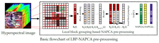
In the joint LBP–NAPCA-based improved non-local spatial sparse unmixing method, the candidate local blocks are dealt with many considerations and pre-process, i.e., groupings and selection, until stable and reliable neighborhood local blocks are obtained and then traditional nonlocal means based spatial sparse unmixing procedure is adopted. The basic flowchart of the LBP–NAPCA pre-processing can be depicted as Figure 2.
Plugging the pre-obtained candidate spatial information into the spatial regularization sparse unmixing model as an improved weight matrix, the propose algorithm can be constructed as (16). To solve the optimization problem (16) of the proposed method, alternating direction method of multipliers (ADMM) is used following the references [28,68], and we would revisit the whole optimization procedure in detail.
Let be the augmented Lagrangian for the minimization objective function:
where μ is a positive constant, acted as an inner Lagrangian multiplier. Let U = X, and U is the newly introduced variable, acted as the estimated fractional abundance matrix, and D = {D1,D2,D3,D4} denoted as a sequence of Lagrangian multipliers associated with the constraint ; In addition, let V = {V1,V2,V3,V4} to simplify the representation of the original part of the object function, G = [A; I; W; I]T, where W is the weight matrix obtained by nonlocal means process for the abundance imagery spatial consideration after local block grouping based noisy-adjusted principal component analysis method, and B = diag(−I); represent the cost function of the following optimization problem:
where .
The implement of the ADMM to solve the optimization problem in the proposed method can be shown as in Algorithm 1.
| Algorithm 1: Pseudocode of the proposed method |
|
4. Experiments with Simulated Data
In this section, the proposed spatial regularization sparse unmixing performance was evaluated using simulated hyperspectral datasets. The classical sparse unmixing approach, i.e., sparse unmixing via variable splitting and augmented Lagrangian (SUnSAL), sparse unmixing via variable splitting and augmented Lagrangian and total variation (SUnSAL-TV), and non-local sparse unmixing (NLSU), are selected to compare with the proposed method. In addition, for quantitative analysis, the signal-to-reconstruction error (SRE), measured in dB, together with the root-mean-square error (RMSE), are used to assess the different performances, which are defined as follows:
where is denoted as the true abundance, and represents the estimated abundance. is the number of pixels in the abundance map. Simultaneously, to compare the efficiency of these different algorithms, the running times are also provided at the end of this section.
4.1. Simulated Datasets
Three simulated datasets are considered in our simulated datasets, which are used as benchmarks in spectral unmixing research. The spectra of these three simulated datasets were randomly selected from the U. S. Geological Survey (USGS) mineral spectra library, given in L = 224 spectral bands and distributed uniformly in the interval 0.4–2.5 μm. In the generative process, the abundance non-negativity constraint (ANC) and abundance sum-to-one constraint (ASC) were enforced.
- (1)
- Simulated Data Cube 1 (DC-1): DC-1 was generated with 75 × 75 pixels and 224 bands per pixel, using a linear mixture model. Five endmembers (shown as Figure 3a) were selected randomly from a standard spectral library, denoted as A (more information can be found at http://speclab.cr.usgs.gov/spectral.lib06). The abundance images were constructed simply, distributed spatially in the form of distinct square regions. Finally, independent and identically distributed (denoted as i.i.d.) Gaussian noise was added with SNR = 30 dB, which means a high intensity noise pollution. The true abundance maps of DC-1 are shown in Figure 3b–f.
- (2)
- Simulated Data Cube 2 (DC-2): DC-2 was provided by Dr. M. D. Iordache and Prof. J. M. Bioucas-Dias, with an image size of 100 × 100 pixels and 224 bands, and acts as a benchmark for spectral unmixing algorithms. In this simulated dataset, nine spectral signatures were selected from the standard spectral library A with spectral angles smaller than 4 degrees, which means they can be easily confused, and then a Dirichlet distribution was utilized uniformly over the probability simplex to obtain the fractional abundance maps, which can exhibit spatial homogeneity better. Finally, i.i.d. Gaussian noise of 30 dB was added. Figure 4 illustrates the true fractional abundance maps as well as the nine spectral curves.
- (3)
- Simulated Data Cube 3 (DC-3): DC-3, with 100 × 100 pixels and 221 bands per pixel, was created for benchmarking the accuracy of the spectral unmixing provided in the HyperMix tool [69]. There are fractal patterns since they can be approximated to a certain degrees, including clouds, mountain ranges, coastlines, vegetables, etc. The endmembers for DC-3 were randomly selected from a USGS library after removing certain bands. In addition, zero-mean Gaussian nose was added with the SNR = 10 dB, which means the poor quality of this data cube. The true abundance maps of the nine endmembers are shown in Figure 5.
4.2. Results and Discussion
Figure 6, Figure 7 and Figure 8 just show part of the estimated fractional abundance images obtained by these three simulated datasets using SUnSAL, SUnSAL-TV, NLSU and the proposed method, respectively. Assessments are made from both the qualitative and quantitative aspects. The SRE, RMSE values, as well as running times are listed in Table 1. The higher the SRE(dB) as well as the lower the RMSE, the better the unmixing performance.
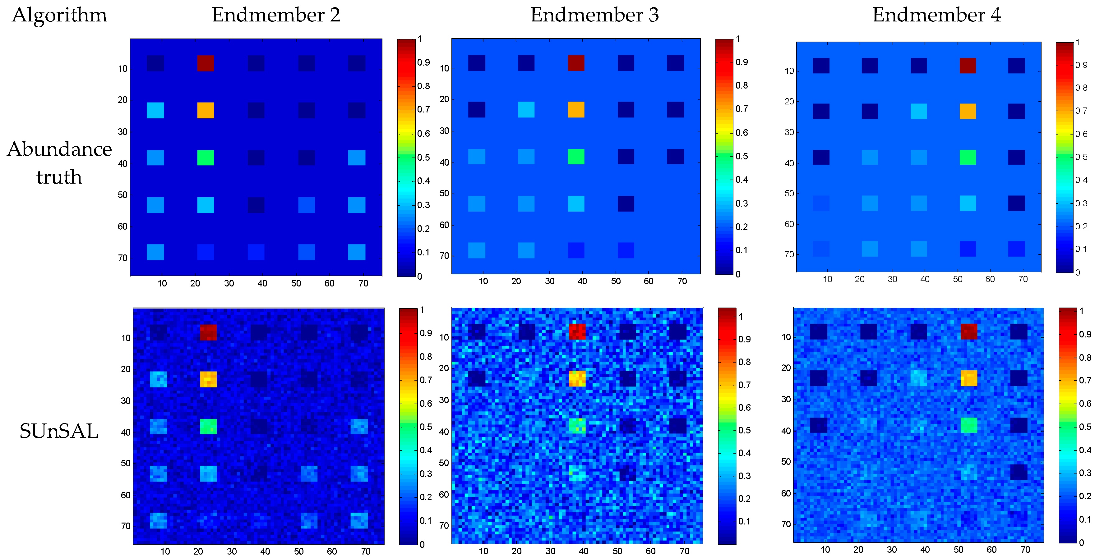
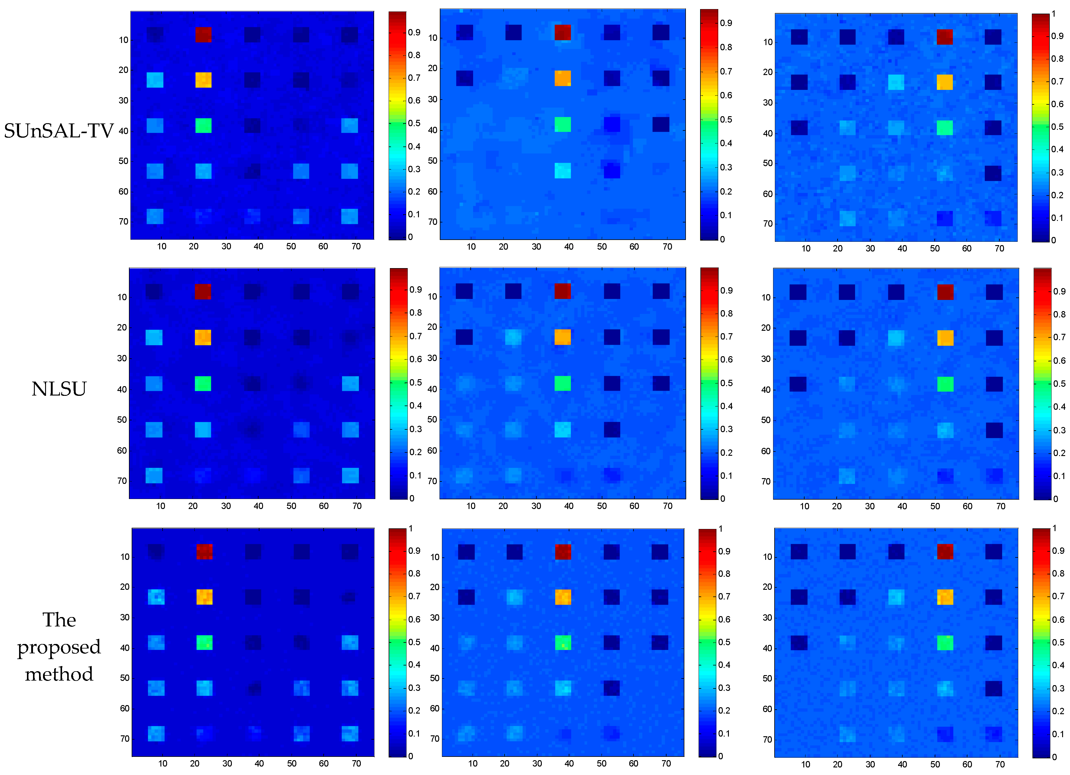
Figure 6 and Figure 7 show the results of abundance images obtained by different spectral unmixing algorithms with DC-1 and DC-2. It can be observed the performance of spectral unmixing has become better from the simple sparse unmixing to the spatial regularization sparse unmixing method. Since total variation spatial regularization sparse hyperspectral unmixing has considered spatial information between neighborhood pixels, the abundance maps obtained by SUnSAL-TV make a significant improvement compared with the abundance maps obtained by SUnSAL. TheNLSU algorithm, acting as a typical second-order neighborhood system spatial regularization sparse unmixing method, seems well-suited for DC-1 and DC-2, which exhibits more smooth background information. The proposed method, which focuses on enhancing the efficiency and reliable spatial correlation, has achieved satisfying unmixing effect. Considering that the proposed method is an upgrade compared with NLSU, it has acquired comparative or even better unmixing results. Set DC-2, endmember 4 as an example, and the abundance map obtained by the proposed method outperforms the fractional map of NLSU. More detailed information can be check in Figure 7. Because of different processing strategies, the estimated fractional abundance values are basically different between NLSU and the proposed method. The most evident difference should lies in the effect of noise. In DC-1, there is lots of scatter noise distributed evenly in the background. After spatial sparse unmixing algorithm processing, the background exhibits different visual effect (e.g., DC-1, endmember 3 and DC-2, endmember 5): SUnSAL-TV has removed high-intensity noise and lost some important information; NLSU has eliminated noise to the greatest extent, but also lost part of information contaminated strongly by noise; The proposed method has handled the advantage of NLSU in suppressing the noise, and also maintains the higher reliable information as much as possible.
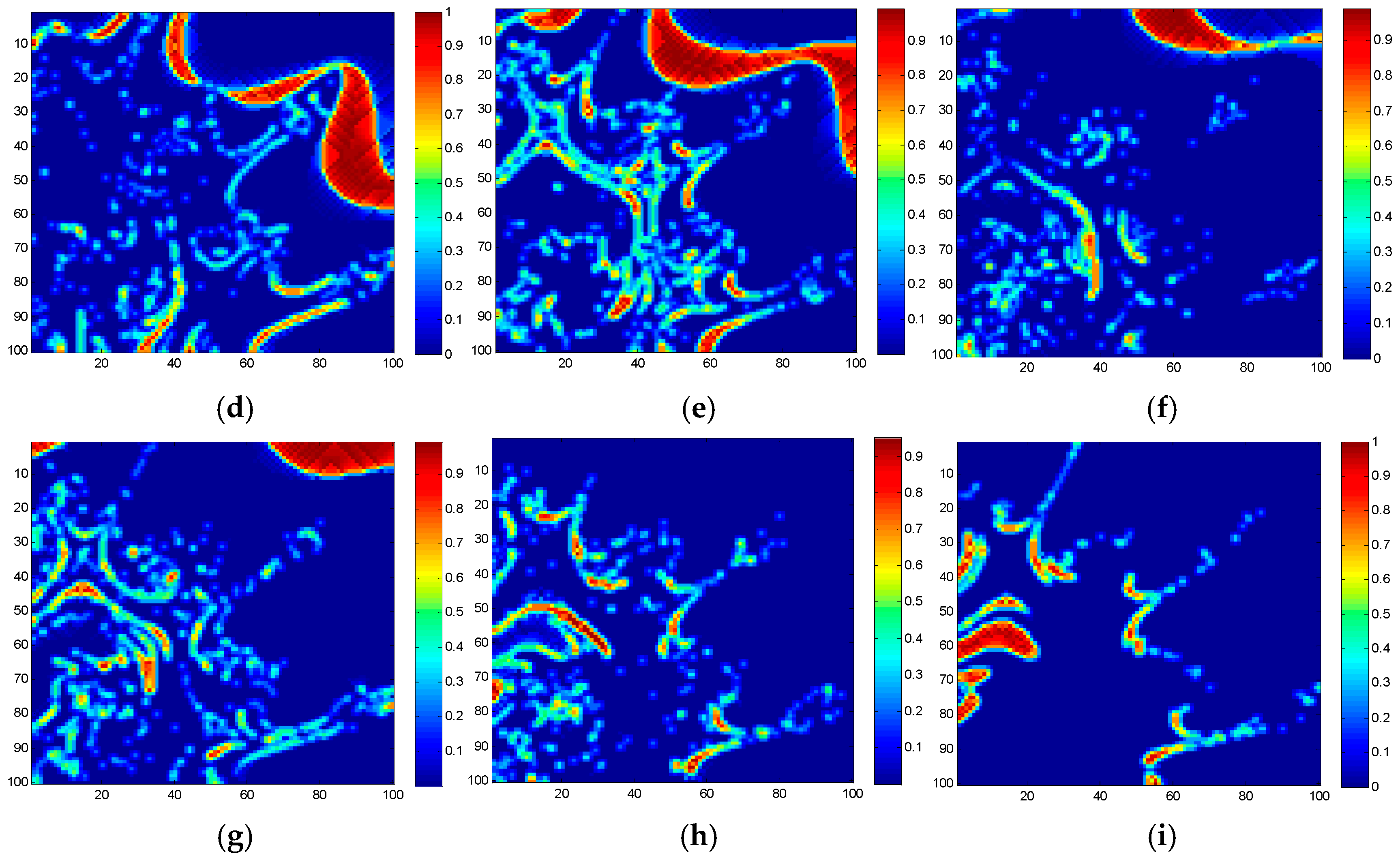
Another simulated dataset experiment can be referred to in Figure 8. Since the abundance maps estimated for DC-3 exhibit similar behavior as DC-1 and DC-2, we only select the estimated fractional abundance maps for endmember 1, 5, and 9 as example. The abundance maps, shown in Figure 8, were all obtained with optimal conditions. From Figure 8, it can be noted SUnSAL-TV, NLSU as well as the proposed method have improved the SUnSAL solution, especially in suppressing the scatter noise in the background and at the edge of regions. Compared with the SUnSAL-TV algorithm, NLSU better maintains structures and detailed information and avoids over-smoothing as shown in SUnSAL-TV for endmember 1. The proposed method keeps the reliable spatial prior information as well as structures and edges firstly and removes some negative spatial blocks at the same time, which makes the homogeneous areas much smoother and better restrains the influence of noise, as endmember 9 of DC-3.
Table 1 gives a comparison of SUnSAL, SUnSAL-TV, NLSU and the proposed method in terms of SRE(dB), RMSE and the running times of each algorithms for the three simulated data cubes.
The SRE(dB) values and the RMSE values are consistent with the visual effects of the obtained fractional abundance maps. The SRE(dB) values obtained by the proposed method are close or a little higher than NLSU algorithm. For DC-1 and DC-2, the proposed method and NLSU provide results which are not quite different, which means the NAPCA-based spatial preprocessing strategy can maintain the precise second-order neighborhood system regularization sparse unmixing algorithm. Note also that for DC-3, the poor quality simulated hyperspectral data cube (SNR = 10dB), the proposed method improves the SRE(dB) value from 9.9868 (NLSU) to 11.1548, and RMSE value decreases from 0.0774 (SUnSAL-TV) to 0.0677, which illustrates the effectiveness of the proposed method.
The running times of the different algorithms for these five datasets are also provided in Table 1, obtained on the MATLAB R2014a platform by a PC equipped with an Intel Core i7-6700 CPU @3.4 GHz and 16 GB RAM. From Table 1, it can be noted that the SUnSAL algorithm is obviously the most efficient one. Owing to the use of tactics such as the core process of NLSU and the proposed method being coded in C++ together with MATLAB, the running times of NLSU and the proposed method have the similar running times as SUnSAL-TV. Owing to the use of local block grouping with the noise-adjusted principal component analysis method, theoretically, the proposed method could able to decrease much computation load in calculating the spatial correlation step, such as the running time of DC-3, the proposed method could converge fast to the approximate optimal solution, within just 37s. However, the NLSU as well as SUnSAL-TV need more time to compute the weight matrix of spatial relationship. However, since the local block grouping idea and the NAPCA process also need to calculate, the running time of the proposed method does not always show a significantly advantage in terms of efficiency, especially for DC-1 and DC-2 datasets, which also take the same amount of running times. But it does make sense in theory that the proposed method should be more efficient. In our further research, there will be more focus on improving the efficiency of the algorithm.
5. Experiments with Real Hyperspectral Imagery
In this section, two real hyperspectral remote-sensing images are chosen to test the proposed spatial regularization sparse unmixing methods. For the first hyperspectral image dataset, the approximate abundance images are obtained by classification with the high-spatial resolution image, while for the latter, the Hyperspectral Digital Imagery Collection Experiment (HYDICE) Urban image, the reference abundance images are coming from [31]. In this paper, different spectral unmixing algorithms are evaluated qualitatively and quantitatively.
5.1. Real Hyperspectral Datasets
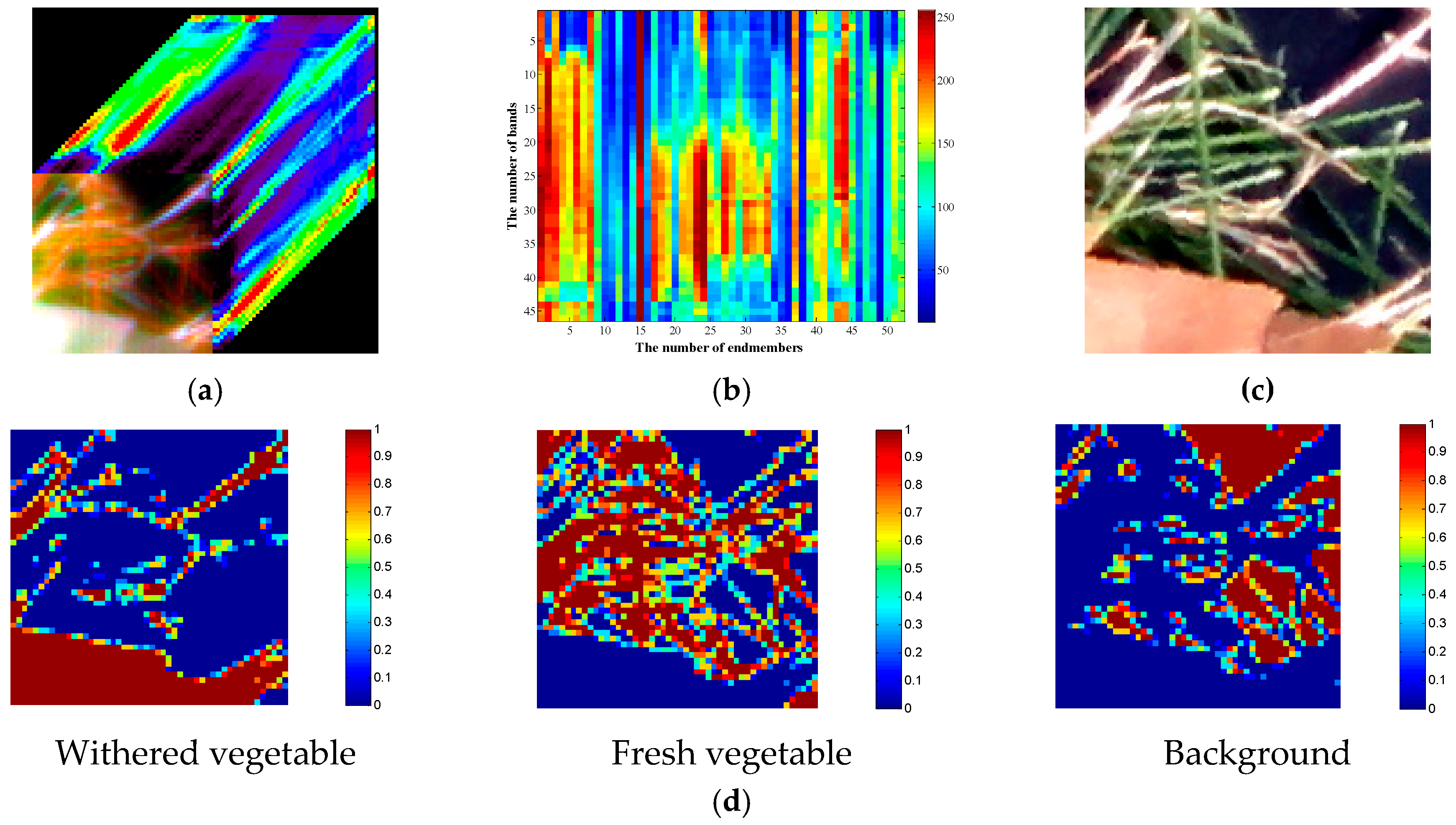
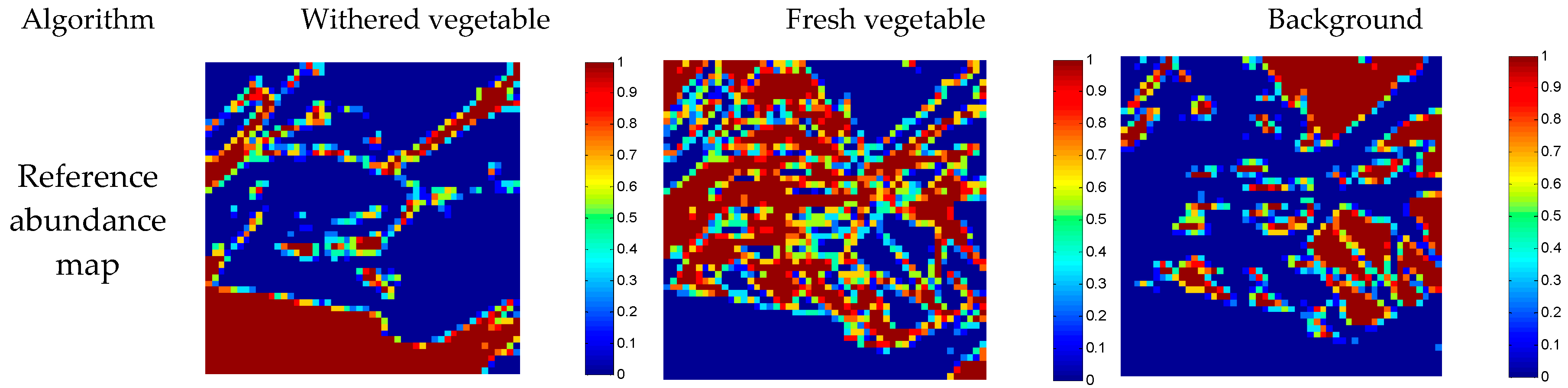
To evaluate the application of the proposed spatial regularized sparse unmixing algorithm in practice, a real experiment was implemented by a simple hyperspectral image (50 × 50 pixels, 46 bands, shown in Figure 9a and denoted as R-1), which was obtained by a Nuance Near-Infrared (NIR) imaging spectrometer, with spectral ranges from 650 nm to 1100 nm, and 10 nm spectral interval. For sparse unmixing algorithms, spectral library acted as prior knowledge for this real hyperspectral image was selected from the hyperspectral images which were also obtained by the Nuance NIR imaging spectrometer as shown in Figure 9b, which contains 52 pure materials as shown on the x-axis, with 46 bands shown on the y-axis in Figure 9b. In addition, the colorbar in Figure 9b denotes the range of digital numbers of this dictionary. To undertake a quantitative assessment, the same scene on the same day using a digital camera was also captured simultaneously in 150 × 150 pixels and red-green-blue (R-G-B) three channels with a higher-spatial resolution (denoted as HR image shown as Figure 9c). After essential preprocessing (geometrical calibration, classification, and down-sampling), the approximate reference abundance maps can be obtained preparing for evaluating the performance of different spectral unmixing methods, shown as Figure 9c. More information about this dataset can be found in [34].
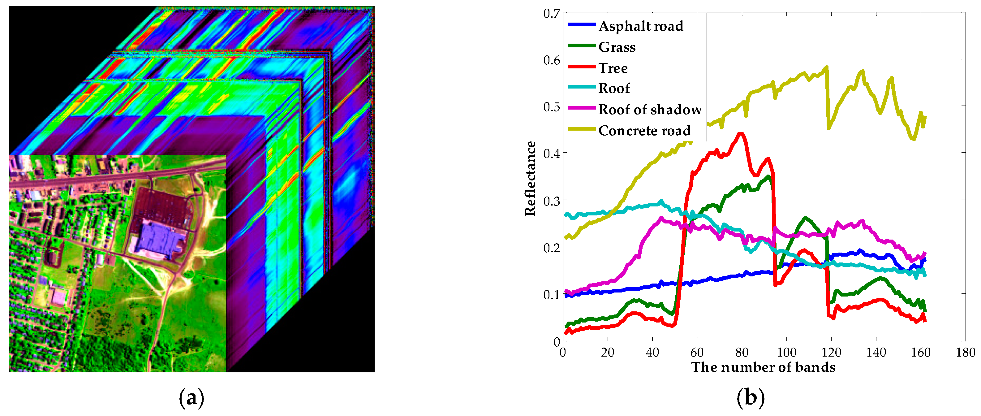
The second real hyperspectral dataset (R-2) was urban data captured by the HYDICE sensor at Copperas Cove near Fort Hood, Texas, U.S., in October 1995, with a size of 307 × 307, 210 bands, as shown in Figure 10a. The spatial and spectral resolutions are 2 m and 10 nm, respectively. Ground objects in this area can be distinguished easily, and six ground objects, including asphalt road, grass, tree, roof, roof shadow, and concrete road would be chosen as the endmembers and used in the spectral unmixing process after analysis [14,31,70], as shown in Figure 10b. The reference ground-truths abundance images are obtained in [31] and displayed as follows in Figure 10c. In addition, some noisy bands with low SNR values had been removed in our experiment.
5.2. Results and Analysis
Figure 11 shows a series of results obtained by different sparse unmixing algorithms for R-1 hyperspectral image. It can be observed that the abundance maps obtained by different approaches exhibit different performance, and the big difference mainly lies in the background. For SUnSAL, the background abundance image is sparse and some of important information has been lost, such as the background in the lower right side. By contrast with SUnSAL, SUnSAL-TV adopts total variation spatial consideration method, which smooths out the spatial details greatly and blurs some of the tiny edges and leads to some homogeneous areas. This method performs well in suppressing wrong unmixing pixels, but bad for image details. NLSU and the proposed method have gained similar unmixing results, which illustrates that the proposed method can better maintain the advantage of the NLSU algorithm. In addition, for some local parts in the abundance images, such as the slender leaves in the upper right corner of the fresh vegetable, a small region of background at the bottom left, the proposed method does a more detailed process.
For R-2, the urban hyperspectral remote-sensing imager, Figure 12 shows the estimated abundances obtained by different spectral unmixing algorithms. The results obtained by SUnSAL, SUnSAL-TV, and NLSU exhibit similar spatial distribution. The big differences are located in the sparsity degree and spatial smoothness. It can be observed that the fractional abundance maps obtained by NLSU are much sparser, which removed many tiny edges and details. In addition, compared with SUnSAL-TV, NLSU enhances the current land cover with higher abundance values. The estimated fractional abundance values acquired by the proposed method are much closer to 1, and shown as a red or deep orange color in Figure 12, which demonstrate the pixels’ physical material type definitely.
Table 2 also provides the SRE(dB) values together with RMSE values and running times of the different algorithms for these two real hyperspectral remote-sensing images. From Table 2, it can be noted that the proposed method has gained a little progress in SRE(dB) values and RMSE assessment for R-1 real hyperspectral images, which is consistent with visual effect. But for R-2 data, the results seem much closer to the reference abundance maps, especially in the areas distributed with many pure pixels, while the quantitative criteria just have slightly increase. The main reason may lie in the poor performance in the regions distributed with mixed materials, such as the bottom part of the asphalt road component obtained by the proposed method. Besides, the running time of the proposed method for R-1 is a little reduced compared with NLSU, which means the effectiveness of the strategies adopted in the proposed method. For R-2, the proposed method is time consuming compared with NLSU. The reason for this phenomenon is the size of R2, which has more than 160 bands as well 307 × 307 pixels. The strategies used in the pre-processing add to the time cost inevitably. In our future research, more tactics should be considered to enhance the calculation efficiency.
6. Conclusions
In this paper, a joint local block grouping with noise-adjusted principal component analysis method has been proposed to enhance the performance of the spatial regularized sparse unmixing method for hyperspectral remote-sensing imagery. In this novel spatial regularized sparse unmixing model, spatial information has been selected by grouping method and noise-adjusted principal component analysis method after rearranging them as local blocks, in which local spatial structures as well as textures can be better maintained and high-quality blocks are selected to consider spatial correlations. Owing to the use of noise-adjusted principal analysis, inaccurate fractional abundances’ local blocks can be dropped and the computation burden is greatly reduced with a constant local block number for spatial consideration. In addition, to verify the effectiveness of the proposed method, experiments with simulated dataset cubes and real remote-sensing hyperspectral images were conducted. From the fractional abundance maps, it can be observed that the proposed method obtains a series of result more similar to ground truth or has a better visual effect. Considering the RMSE and SRE, the proposed approach outperformed the traditional sparse or spatial regularized sparse unmixing algorithms.
Author Contributions
All of the authors made significant contributions to the work. R.F. designed the research, analyzed the results, and accomplished the validation work. L.W. gave advice on the methodology and paper revision. Y.Z. provided advice for the revision of the paper and revised the final manuscript.
Funding
This work was supported in part by the Fundamental Research Funds for the Central Universities, China University of Geosciences (Wuhan) (Grant No. CUG170625); in part by the National Natural Science Foundation of China (Grant No. 41701429); in part by the Open Research Project of The Hubei Key Laboratory of Intelligent Geo-Information Processing (KLIGIP-2017B08); and in part by the Open Research Fund of the Key Laboratory of Spectral Imaging Technology, Chinese Academy of Sciences (Grant No. LSIT201716D).
Acknowledgments
The authors would like to thank the research group supervised by J. M. Bioucas-Dias and A. Plaza for sharing the simulated datasets and the source code of the latest sparse algorithms with the community, together with the free downloads of the AVIRIS image. The authors would also like to thank F. Zhu, C. Pan and S. Xiang for sharing HYDICE Urban dataset and ground truths. The authors also highly appreciate the time and consideration of editors, anonymous referees, and English language editors for their constructive suggestions that greatly improved the paper.
Conflicts of Interest
The authors declare no conflict of interest. The founding sponsors had no role in the design of the study; in the collection, analyses, or interpretation of data; in the writing of the manuscript; or in the decision to publish the results.
References
- Ghamisi, P.; Yokoya, N.; Li, J.; Liao, W.; Liu, S.; Plaza, J.; Rasti, B.; Plaza, A. Advances in hyperspectral image and signal processing. IEEE Geosci. Remote Sens. Mag. 2017, 5, 37–78. [Google Scholar] [CrossRef]
- Tong, Q.; Xue, Y.; Zhang, L. Progress in hyperspectral remote sensing science and technology in China over the past three decades. IEEE J. Sel. Top. Appl. Earth Observ. Remote Sens. 2014, 7, 70–91. [Google Scholar] [CrossRef]
- Li, C.; Liu, Y.; Cheng, J.; Song, R.; Peng, H.; Chen, Q.; Chen, X. Hyperspectral unmixing with bandwise generalized bilinear model. Remote Sens. 2018, 10, 1600. [Google Scholar] [CrossRef]
- Wang, Q.; Yuan, Z.; Du, Q.; Li, X. GETNET: A general end-to-end two-dimensional CNN framework for hyperspectral image change detection. IEEE Trans. Geosci. Remote Sens. 2019, 57, 3–13. [Google Scholar] [CrossRef]
- Luo, H.; Liu, C.; Wu, C.; Guo, X. Urban change detection based on dempster-shafer theory for multi-temporal very high-resolution imagery. Remote Sens. 2018, 10, 980. [Google Scholar] [CrossRef]
- Luo, H.; Wang, L.; Wu, C.; Zhang, L. An improved method for impervious surface mapping incorporating LiDAR data and high-resolution imagery at different acquisition times. Remote Sens. 2018, 10, 1349. [Google Scholar] [CrossRef]
- Liu, J.; Luo, B.; Doute, S.; Chanussot, J. Exploration of planetary hyperspectral images with unsupervised spectral unmixing: A case study of planet Mars. Remote Sens. 2018, 10, 737. [Google Scholar] [CrossRef]
- Marcello, J.; Eugenio, F.; Martin, J.; Marques, F. Seabed mapping in coastal shallow waters using high resolution multispectral and hyperspectral imagery. Remote Sens. 2018, 10, 1208. [Google Scholar] [CrossRef]
- Zhang, X.; Li, C.; Zhang, J.; Chen, Q.; Feng, J.; Jiao, L.; Zhou, H. Hyperspectral unmixing via low-rank representation with sparse consistency constraint and spectral library pruning. Remote Sens. 2018, 10, 339. [Google Scholar] [CrossRef]
- Salehani, Y.E.; Gazor, S.; Cheriet, M. Sparse hyperspectral unmixing via heuristic lp-norm approach. IEEE J. Sel. Top. Appl. Earth Observ. Remote Sens. 2018, 11, 1191–1202. [Google Scholar] [CrossRef]
- Shi, C.; Wang, L. Linear spatial spectral mixture model. IEEE Trans. Geosci. Remote Sens. 2016, 54, 3599–3611. [Google Scholar] [CrossRef]
- Bioucas-Dias, J.M.; Plaza, A.; Camps-Valls, G.; Scheunders, P.; Nasrabadi, N.M.; Chanussot, J. Hyperspectral remote sensing data analysis and future challenges. IEEE Geosci. Remote Sens. Mag. 2013, 1, 6–36. [Google Scholar] [CrossRef]
- Nascimento, J.M.P.; Bioucas-Dias, J.M. Does independent component analysis play a role in unmixing hyperspectral data? IEEE Trans. Geosci. Remote Sens. 2005, 43, 175–187. [Google Scholar] [CrossRef]
- Liu, X.; Xia, W.; Wang, B.; Zhang, L. An approach based on constrained nonnegative matrix factorization to unmix hyperspectral data. IEEE Trans. Geosci. Remote Sens. 2011, 49, 757–772. [Google Scholar] [CrossRef]
- Wang, M.; Zhang, B.; Pan, X.; Yang, S. Group low-rank nonnegative matrix factorization with semantic regularizer for hyperspectral unmixing. IEEE J. Sel. Top. Appl. Earth Observ. Remote Sens. 2018, 11, 1022–1029. [Google Scholar] [CrossRef]
- Fang, H.; Li, A.; Xu, H.; Wang, T. Sparsity-constrained deep nonnegative matrix factorization for hyperspectral unmixing. IEEE Geosci. Remote Sens. Lett. 2018, 15, 1105–1109. [Google Scholar] [CrossRef]
- Bioucas-Dias, J.M.; Plaza, A.; Dobigeon, N.; Parente, M.; Du, Q.; Gader, P.; Chanussot, J. Hyperspectral unmixing overview: Geometrical, statistical, and sparse regression-based approaches. IEEE J. Sel. Top. Appl. Earth Observ. Remote Sens. 2012, 5, 354–379. [Google Scholar] [CrossRef]
- Hendrix, E.M.T.; Garcia, I.; Plaza, J.; Martin, G.; Plaza, A. A new minimum-volume enclosing algorithm for endmember identification and abundance estimation in hyperspectral data. IEEE Trans. Geosci. Remote Sens. 2012, 50, 2744–2757. [Google Scholar] [CrossRef]
- Somers, B.; Zortea, M.; Plaza, A.; Asner, G. Automated extraction of image-based endmember bundles for improved spectral unmixing. IEEE J. Sel. Top. Appl. Earth Observ. Remote Sens. 2012, 5, 396–408. [Google Scholar] [CrossRef]
- Cohen, J.E.; Gillis, N. Spectral unmixing with multiple dictionaries. IEEE Geosci. Remote Sens. Lett. 2018, 15, 187–191. [Google Scholar] [CrossRef]
- Xu, X.; Tong, X.; Plaza, A.; Zhong, Y.; Xie, H.; Zhang, L. Joint sparse sub-pixel model with endmember variability for remotely sensed imagery. Remote Sens. 2017, 9, 15. [Google Scholar] [CrossRef]
- Fu, X.; Ma, W.-K.; Bioucas-Dias, J.M.; Chan, T.-H. Semiblind hyperspectral unmixing in the presence of spectral library mismatches. IEEE Trans. Geosci. Remote Sens. 2016, 54, 5171–5184. [Google Scholar] [CrossRef]
- Thouvenin, P.-A.; Dobigeon, N.; Tourneret, J.-Y. Hyperspectral unmixing with spectral variability using a perturbed linear mixing model. IEEE Trans. Signal. Process. 2016, 64, 525–538. [Google Scholar] [CrossRef]
- Drumetz, L.; Veganzones, M.-A.; Henrot, S.; Phlypo, R.; Chanussot, J.; Jutten, C. Blind hyperspectral unmixing using an entended linear mixing model to address spectral variability. IEEE Trans. Image Process. 2016, 25, 3890–3905. [Google Scholar] [CrossRef]
- Hong, D.; Yokoya, N.; Chanussot, J.; Zhu, X.-X. An augmented linear mixing model to address spectral variability for hyperspectral unmixing. IEEE Trans. Image Process. 2019, 28, 1923–1938. [Google Scholar] [CrossRef]
- Drumetz, L.; Meyer, T.R.; Chanussot, J.; Bertozzi, A.L.; Jutten, C. Hyperspectral image unmixing with endmember bundles and group sparsity inducing mixed norms. IEEE Trans. Image Process. 2019. [Google Scholar] [CrossRef] [PubMed]
- Hong, D.; Zhu, X.-X. SULoRA: Subspace unmixing with low rank attribute embedding for hyperspectral data analysis. IEEE J. Sel. Top. Signal. Process. 2018, 12, 1351–1363. [Google Scholar] [CrossRef]
- Bioucas-Dias, J.M.; Figueiredo, M. Alternating direction algorithms for constrained sparse regression: Application to hyperspectral unmixing. In Proceedings of the 2nd IEEE GRSS Workshop on Hyperspectral Image and Signal Processing: Evolution in Remote Sensing (WHISPERS), Reykjavik, Iceland, 14–16 June 2010. [Google Scholar]
- Iordache, M.D. A Sparse Regression Approach to Hyperspectral Unmixing. Ph.D. Thesis, School of Electrical and Computer Engineering, Ithaca, NY, USA, 2011. [Google Scholar]
- Rizkinia, M.; Okuda, M. Joint local abundance sparse unmixing for hyperspectral images. Remote Sens. 2017, 9, 1224. [Google Scholar] [CrossRef]
- Zhu, F.; Wang, Y.; Xiang, S.; Fan, B.; Pan, C. Structured sparse method for hyperspectral unmixing. ISPRS J. Photogramm. Remote Sens. 2014, 88, 101–118. [Google Scholar] [CrossRef]
- Bruckstein, A.M.; Elad, M.; Zibulevsky, M. On the uniqueness of nonnegative sparse solutions to underdetermined systems of equations. IEEE Trans. Inf. Theory 2008, 54, 4813–4820. [Google Scholar] [CrossRef]
- Candes, E.; Romberg, J.J. Sparsity and incoherence in compressive sampling. IEEE Trans. Image Process. 2007, 23, 969–985. [Google Scholar] [CrossRef] [Green Version]
- Pati, Y.C.; Rezaiifar, R.; Krishnaprasad, P. Orthogonal matching pursuit: Recursive function approximation with applications to wavelet decomposition. In Proceedings of the 27th Asilomar Conference on Signals, Systems and Computers, Pacific Grove, CA, USA, 1–3 November 1993; pp. 40–44. [Google Scholar]
- Iordache, M.D.; Bioucas-Dias, J.M.; Plaza, A. Sparse unmixing of hyperspectral data. IEEE Trans. Geosci. Remote Sens. 2011, 49, 2014–2039. [Google Scholar] [CrossRef]
- Li, C.; Ma, Y.; Mei, X.; Fan, F.; Huang, J.; Ma, J. Sparse unmixing of hyperspectral data with noise level estimation. Remote Sens. 2017, 9, 1166. [Google Scholar] [CrossRef]
- Feng, R.; Wang, L.; Zhong, Y. Least angle regression-based constrained sparse unmixing of hyperspectral remote sensing imagery. Remote Sens. 2018, 10, 1546. [Google Scholar] [CrossRef]
- Iordache, M.D.; Bioucas-Dias, J.M.; Plaza, A. Total variation spatial regularization for sparse hyperspectral unmixing. IEEE Trans. Geosci. Remote Sens. 2012, 50, 4484–4502. [Google Scholar] [CrossRef]
- Zhong, Y.; Feng, R.; Zhang, L. Non-local sparse unmixing for hyperspectral remote sensing imagery. IEEE J. Sel. Top. Appl. Earth Observ. Remote Sens. 2014, 7, 1889–1909. [Google Scholar] [CrossRef]
- Iordache, M.D.; Bioucas-Dias, J.M.; Plaza, A. Collaborative sparse regression for hyperspectral unmixing. IEEE Trans. Geosci. Remote Sens. 2014, 52, 341–354. [Google Scholar] [CrossRef]
- Iordache, M.D.; Bioucas-Dias, J.M.; Plaza, A.; Somers, B. MUSIC-CSR: Hyperspectral unmixing via multiple signal classification and collaborative sparse regression. IEEE Trans. Geosci. Remote Sens. 2014, 52, 4364–4382. [Google Scholar] [CrossRef]
- Feng, R.; Zhong, Y.; Zhang, L. Adaptive non-local Euclidean medians sparse unmixing for hyperspectral imagery. ISPRS J. Photogramm. Remote Sens. 2014, 97, 9–24. [Google Scholar] [CrossRef]
- Feng, R.; Zhong, Y.; Zhang, L. Adaptive spatial regularization sparse unmixing strategy based on joint MAP for hyperspectral remote sensing imagery. IEEE J. Sel. Top. Appl. Earth Observ. Remote Sens. 2016, 9, 5791–5805. [Google Scholar] [CrossRef]
- Zhang, S.; Li, J.; Li, H.; Deng, C.; Plaza, A. Spectral-spatial weighted sparse regression for hyperspectral image unmixing. IEEE Trans. Geosci. Remote Sens. 2018, 56, 3265–3276. [Google Scholar] [CrossRef]
- Wang, S.; Huang, T.; Zhao, X.; Liu, G.; Cheng, Y. Double reweighted sparse regression and graph regularization for hyperspectral unmixing. Remote Sens. 2018, 10, 1046. [Google Scholar] [CrossRef]
- Rudin, L.; Osher, S.; Fatemi, E. Nonlinear total variation based noise removal algorithms. Phys. D Nonlinear Phenom. 1992, 60, 259–268. [Google Scholar] [CrossRef]
- Xiong, F.; Qian, Y.; Zhou, J.; Tang, Y. Hyperspectral unmixing via total variation regularized nonnegative tensor factorization. IEEE Trans. Geosci. Remote Sens. 2019, 57, 2341–2357. [Google Scholar] [CrossRef]
- Wang, Q.; He, X.; Li, X. Locality and structure regularized low rank representation for hyperspectral image classification. IEEE Trans. Geosci. Remote Sens. 2019, 57, 911–923. [Google Scholar] [CrossRef]
- Feng, R.; Zhong, Y.; Zhang, L. An improved nonlocal sparse unmixing algorithm for hyperspectral imagery. IEEE Geosci. Remote Sens. Lett. 2015, 12, 915–919. [Google Scholar] [CrossRef]
- Wang, R.; Li, H.; Liao, W.; Huang, X.; Philips, W. Centralized collaborative sparse unmixing for hyperspectral images. IEEE J. Sel. Top. Appl. Earth Observ. Remote Sens. 2017, 10, 1949–1962. [Google Scholar] [CrossRef]
- Wang, S.; Wang, C.M.; Chang, M.L.; Tsai, C.T.; Chang, C.I. Applications of kalman filtering to single hyperspectral signature analysis. IEEE Sens. J. 2010, 10, 547–563. [Google Scholar] [CrossRef]
- Zhang, S.; Li, J.; Wu, Z.; Plaza, A. Spatial discontinuity-weighted sparse unmixing of hyperspectral images. IEEE Trans. Geosci. Remote Sens. 2018, 56, 5767–5779. [Google Scholar] [CrossRef]
- Cai, J.F.; Osher, S.; Shen, Z. Convergence of the linearized Bregman iteration for l1-norm minimization. Math. Comput. 2009, 78, 2127–2136. [Google Scholar] [CrossRef]
- Zhang, X.; Burger, M.; Bresson, X.; Osher, S. Bregmanized nonlocal regularization for deconvolution and sparse reconstruction. SIAM J. Imaging Sci. 2010, 3, 253–276. [Google Scholar] [CrossRef]
- Lee, J.B.; Woodyatt, A.S.; Berman, M. Enhancement of high spectral resolution remote sensing data by a noise-adjusted principal components transform. IEEE Trans. Geosci. Remote Sens. 1990, 28, 295–304. [Google Scholar] [CrossRef]
- Roger, R.E. A fast way to compute the noise-adjusted principal components transform matrix. IEEE Trans. Geosci. Remote Sens. 1994, 32, 1194–1196. [Google Scholar] [CrossRef]
- Chang, C.I.; Du, Q. Interference and noise-adjusted principal components analysis. IEEE Trans. Geosci. Remote Sens. 1999, 37, 2387–2396. [Google Scholar] [CrossRef] [Green Version]
- Mohan, A.; Sapiro, G.; Bosch, E. Spatially coherent nonlinear dimensionality reduction and segmentation of hyperspectral images. IEEE Geosci. Remote Sens. Lett. 2007, 4, 206–210. [Google Scholar] [CrossRef]
- Li, X.; Wang, G. Optimal band selection for hyperspectral data with improved differential evolution. J. Ambient Intell. Hum. Comput. 2015, 6, 675–688. [Google Scholar] [CrossRef]
- Chaib, S.; Liu, H.; Gu, Y.; Yao, H. Deep feature fusion for VHR remote sensing scene classification. IEEE Trans. Geosci. Remote Sens. 2017, 55, 4775–4784. [Google Scholar] [CrossRef]
- Wang, L.; Song, W.; Liu, P. Link the remote sensing big data to the image features via wavelet transformation. Cluster Comput. 2016, 19, 793–810. [Google Scholar] [CrossRef]
- Chaudhury, K.N.; Singer, A. Non-local Euclidean medians. IEEE Signal. Proc. Lett. 2012, 19, 745–748. [Google Scholar] [CrossRef]
- Pan, S.; Wu, J.; Zhu, X.; Zhang, C. Graph ensemble boosting for imbalanced noisy graph stream classification. IEEE Trans. Cybern. 2015, 45, 954–968. [Google Scholar]
- Wu, J.; Wu, B.; Pan, S.; Wang, H.; Cai, Z. Locally weighted learning: How and when does it work in Bayesian networks? Int. J. Comput. Int. Sys. 2015, 8, 63–74. [Google Scholar] [CrossRef]
- Wu, J.; Pan, S.; Zhu, X.; Cai, Z.; Zhang, P.; Zhang, C. Self-adaptive attribute weighting for Naive Bayes classification. Expert Syst. Appl. 2015, 42, 1478–1502. [Google Scholar] [CrossRef]
- Buades, A.; Coll, B.; Morel, J.M. A review of image denoising algorithm, with a new one. Multiscale Model. Sim. 2005, 4, 490–530. [Google Scholar] [CrossRef]
- Zhang, L.; Dong, W.; Zhang, D.; Shi, G. Two-stage image denoising by principal component analysis with local pixel grouping. Pattern Recogn. 2010, 43, 1531–1549. [Google Scholar] [CrossRef] [Green Version]
- Eckstein, J.; Bertsekas, D. On the Douglas-Rechford splitting method and the proximal point algorithm for maximal monotone operators. Math. Program. 1992, 55, 293–318. [Google Scholar] [CrossRef]
- Jimenez, L.I.; Martin, G.; Plaza, A. A new tool for evaluating spectral unmixing applications for remotely sensed hyperspectral image analysis. In Proceedings of the International Conference Geographic Object-Based Image Analysis (GEOBIA), Rio de Janeiro, Brazil, 7–9 May 2012; pp. 1–5. [Google Scholar]
- Zhong, Y.; Wang, X.; Zhao, L.; Feng, R.; Zhang, L.; Xu, Y. Blind spectral unmixing based on sparse component analysis for hyperspectral remote sensing imagery. ISPRS J. Photogramm. Remote Sens. 2016, 119, 49–63. [Google Scholar] [CrossRef]
Figure 1.
Illustration of basic concept of local block grouping.

Figure 2.
Basic flowchart of local block grouping–noise-adjusted principal component analysis (LBP–NAPCA) pre-processing.
Figure 2.
Basic flowchart of local block grouping–noise-adjusted principal component analysis (LBP–NAPCA) pre-processing.

Figure 3.
Simulated Data Cube 1 (DC-1). (a) The five spectra. (b) Abundance map of #1. (c) Abundance map of #2. (d) Abundance map of #3. (e) Abundance map of #4. (f) Abundance map of #5.
Figure 3.
Simulated Data Cube 1 (DC-1). (a) The five spectra. (b) Abundance map of #1. (c) Abundance map of #2. (d) Abundance map of #3. (e) Abundance map of #4. (f) Abundance map of #5.

Figure 4.
Simulated Data Cube 2 (DC-2). (a) Abundance map of #1. (b) Abundance map of #2. (c) Abundance map of #3. (d) Abundance map of #4. (e) Abundance map of #5. (f) Abundance map of #6. (g) Abundance map of #7. (h) Abundance map of #8. (i) Abundance map of #9. (j) The nine spectral curves.
Figure 4.
Simulated Data Cube 2 (DC-2). (a) Abundance map of #1. (b) Abundance map of #2. (c) Abundance map of #3. (d) Abundance map of #4. (e) Abundance map of #5. (f) Abundance map of #6. (g) Abundance map of #7. (h) Abundance map of #8. (i) Abundance map of #9. (j) The nine spectral curves.


Figure 5.
Simulated Data Cube 3 (DC-3). (a) Abundance map of #1. (b) Abundance map of #2. (c) Abundance map of #3. (d) Abundance map of #4. (e) Abundance map of #5. (f) Abundance map of #6. (g) Abundance map of #7. (h) Abundance map of #8. (i) Abundance map of #9.
Figure 5.
Simulated Data Cube 3 (DC-3). (a) Abundance map of #1. (b) Abundance map of #2. (c) Abundance map of #3. (d) Abundance map of #4. (e) Abundance map of #5. (f) Abundance map of #6. (g) Abundance map of #7. (h) Abundance map of #8. (i) Abundance map of #9.


Figure 6.
Estimated abundances of endmembers for DC-1.


Figure 7.
Estimated abundances of the endmembers for DC-2.

Figure 8.
Estimated abundances of the endmembers for DC-3.

Figure 9.
R-1. (a) R-1-hyperspectral dataset. (b) Spectral library. (c) HR image. (d) Reference abundances.
Figure 9.
R-1. (a) R-1-hyperspectral dataset. (b) Spectral library. (c) HR image. (d) Reference abundances.

Figure 10.
Hyperspectral Digital Imagery Collection Experiment (HYDICE) Urban. (a) R-2. (b) Reference endmember signatures. (c) Reference abundances.
Figure 10.
Hyperspectral Digital Imagery Collection Experiment (HYDICE) Urban. (a) R-2. (b) Reference endmember signatures. (c) Reference abundances.


Figure 11.
Estimated abundances of the three components for R-1.


Figure 12.
Unmixing results for R-2.


Table 1.
Performance comparison for the different methods with the three simulated data cubes.
| Data | Algorithm | SUnSAL | SUnSAL-TV | NLSU | The Proposed Method |
|---|---|---|---|---|---|
| DC-1 | SRE (dB) | 15.1471 | 25.8333 | 29.6473 | 29.9368 |
| RMSE | 0.0421 | 0.0123 | 0.0079 | 0.0077 | |
| Time (s) | 0.4281 | 30.4375 | 19.5000 | 19.0945 | |
| DC-2 | SRE (dB) | 8.0355 | 12.5867 | 15.5208 | 15.7318 |
| RMSE | 0.1007 | 0.0597 | 0.0426 | 0.0415 | |
| Time (s) | 5.4388 | 63.6796 | 64.1788 | 63.9755 | |
| DC-3 | SRE (dB) | 4.5724 | 8.2779 | 9.9863 | 11.1548 |
| RMSE | 0.1444 | 0.0943 | 0.0774 | 0.0677 | |
| Time (s) | 2.9531 | 43.4063 | 73.7885 | 36.2213 |
Note: The highest signal-to-reconstruction error (SRE) and lowest root-mean-square error (RMSE) values in the table are marked in bold.
Table 2.
Performance comparison for the different methods with the two real hyperspectral datasets.
| Data | Algorithm | SUnSAL | SUnSAL-TV | NLSU | The Proposed Method |
|---|---|---|---|---|---|
| R-1 | SRE(dB) | 4.928 | 5.309 | 6.002 | 6.084 |
| RMSE | 0.3051 | 0.2920 | 0.2696 | 0.2671 | |
| Time (s) | 2.9233 | 9.7656 | 270.9219 | 168.0189 | |
| R-2 | SRE(dB) | 8.6392 | 8.6937 | 8.7174 | 8.7408 |
| RMSE | 0.1240 | 0.1232 | 0.1228 | 0.1225 | |
| Time (s) | 133.1875 | 642.3750 | 586.9375 | 639.1004 |
Note: The highest SRE and lowest RMSE values in the table are marked in bold.
© 2019 by the authors. Licensee MDPI, Basel, Switzerland. This article is an open access article distributed under the terms and conditions of the Creative Commons Attribution (CC BY) license (http://creativecommons.org/licenses/by/4.0/).
Share and Cite
MDPI and ACS Style
Feng, R.; Wang, L.; Zhong, Y. Joint Local Block Grouping with Noise-Adjusted Principal Component Analysis for Hyperspectral Remote-Sensing Imagery Sparse Unmixing. Remote Sens. 2019, 11, 1223. https://doi.org/10.3390/rs11101223
AMA Style
Feng R, Wang L, Zhong Y. Joint Local Block Grouping with Noise-Adjusted Principal Component Analysis for Hyperspectral Remote-Sensing Imagery Sparse Unmixing. Remote Sensing. 2019; 11(10):1223. https://doi.org/10.3390/rs11101223
Chicago/Turabian StyleFeng, Ruyi, Lizhe Wang, and Yanfei Zhong. 2019. "Joint Local Block Grouping with Noise-Adjusted Principal Component Analysis for Hyperspectral Remote-Sensing Imagery Sparse Unmixing" Remote Sensing 11, no. 10: 1223. https://doi.org/10.3390/rs11101223
Note that from the first issue of 2016, this journal uses article numbers instead of page numbers. See further details here.