Explorative Study on Mapping Surface Facies of Selected Glaciers from Chandra Basin, Himalaya Using WorldView-2 Data


1
Earth System Science Organization—National Centre for Polar and Ocean Research (ESSO-NCPOR), Ministry of Earth Sciences, Government of India, Headland Sada, Vasco-da-Gama, Goa 403804, India
2
Svalbard Integrated Arctic Earth Observing System (SIOS), SIOS Knowledge Centre, Svalbard Science Centre, P.O. Box 156, N-9171 Longyearbyen, Svalbard, Norway
3
Department of Marine Geology, Mangalore University, Mangalagangotri, Karnataka 574199, India
*
Author to whom correspondence should be addressed.
Remote Sens. 2019, 11(10), 1207; https://doi.org/10.3390/rs11101207
Submission received: 3 April 2019
/
Revised: 22 April 2019
/
Accepted: 26 April 2019
/
Published: 21 May 2019
(This article belongs to the Section Remote Sensing Image Processing)
Abstract
:Mapping of surface glacier facies has been a part of several glaciological applications. The study of glacier facies in the Himalayas has gained momentum in the last decade owing to the implications imposed by these facies on the melt characteristics of the glaciers. Some of the most commonly reported surface facies in the Himalayas are snow, ice, ice mixed debris, and debris. The precision of the techniques used to extract glacier facies is of high importance, as the result of many cryospheric studies and economic reforms rely on it. An assessment of a customized semi-automated protocol against conventional and advanced mapping algorithms for mapping glacier surface facies is presented in this study. Customized spectral index ratios (SIRs) are developed for effective extraction of surface facies using thresholding in an object-based environment. This method was then tested on conventional and advanced classification algorithms for an evaluation of the mapping accuracy for five glaciers located in the Himalayas, using very high-resolution WorldView-2 imagery. The results indicate that the object-based image analysis (OBIA) based semi-automated SIR approach achieved a higher average overall accuracy of 87.33% (κ = 0.85) than the pixel-based image analysis (PBIA) approach. Among the conventional methods, the Maximum Likelihood performed the best, with an overall accuracy of 78.71% (κ = 0.75). The Constrained Energy Minimization, with an overall accuracy of 68.76% (κ = 0.63), was the best performer of the advanced algorithms. The advanced methods greatly underperformed in this study. The proposed SIRs show a promise in the mapping of minor features such as crevasses and in the discrimination between ice-mixed debris and debris. We have efficiently mapped surface glacier facies independently of short-wave infrared bands (SWIR). There is a scope for the transferability of the proposed SIRs and their performance in varying scenarios.
1. Introduction
Snow accumulated on a glacier will metamorphose into ice on exposure to meteorological and geological alterations. This transformation leads to superficial expressions on the surface of the glacier and these expressions are as diverse in attributes as the processes that mold this transformation are intricate. These expressions are known as facies. The structural differences in these facies permit their individual detection and identification. Several facies on annexation categorically fall under two general zonations of a glacier, viz., the zone of accumulation and the zone of ablation. The equilibrium line altitude (ELA) is the line of differentiation between the two. Benson [1] originally described these facies through observations on the Greenland ice sheet, while Paterson [2] later elaborated upon these descriptions. Every facies is unique in terms of both, its spatial variance, and its physical and chemical characteristics. Therefore, it is inevitable that each facies will have a unique impact on the mechanics of the glacier. The changing dimensions of glacier facies affect the processes of deglaciation and these effects vary year-round as the facies themselves vary in either dimension or distribution [3]. However, the term “glacier facies” is used to describe a vast variety of zonations encompassed within the ablation and accumulation zones. Surface classes, however, are representative zonations of facies distinguishable from the surface [4]. Therefore, this study herein uses the term surface glacier facies.
A comprehensive investigation of glacial phenomena is achieved by modeling of the mass balance [5]. In doing so, distributed energy modeling [6,7,8,9,10,11,12] and degree-day modeling [13,14,15,16] are two methods used extensively. The utilization of surface glacier facies to calibrate and validate distributed mass balance models [17] enables the 3-dimensional filling of void sites in such models. Empty cells or void sites within such models are a result of very limited in-situ data collection points that do not fully realize the complexity of glacial processes. Building such a complex model places a requisite for extraction of precise glacier facies. Expensive logistics and inclement weather do not permit such extensive in situ mapping. Hence, remote sensing is a much more globally applicable alternative.
1.1. Glacier Facies via Remote Sensing
Remote identification and extraction of surface glacier facies necessitates an emphasis on quality spectral as well as spatial resolution. Multispectral satellite imagery provides a wide range of techniques and alternatives for demonstrating the extraction of available glacier facies [18,19,20,21,22,23,24]. Radar and its associated approaches have been widely employed in this domain [25,26,27,28,29,30]. Some of the early developmental techniques for the extraction of glacier facies relied on singular datasets, such as the European remote sensing (ERS) satellites, i.e. ERS 1 and ERS 2 imagery [30,31] and Landsat Thematic Mapper (TM)/Multispectral Scanner (MSS) [22,24,32]. Singular use of the visual to near infrared (VNIR) and short wave infrared (SWIR) component of the Advanced Spaceborne Thermal Emission and Reflection Radiometer (ASTER) sensor has also been demonstrated [33]. However, a large number of studies have now begun to integrate varying sensors, data products, field spectra, and freely available digital elevation models (DEMs) into pixel- and object-based environments to extract surface glacier facies [34,35,36,37,38,39,40]. These studies provide a vast working knowledge base to design and implement an effective facies mapping technique. Although the accurate mapping of glacier facies is incorporated into a large number of glaciological studies [3], a relatively fewer number of studies have focused solely on the mapping of glacier facies. This study aims to singularly outline a robust and promising technique for mapping of glacier facies by first examining classification techniques.
Image classification is easily the most widely adopted approach for information extraction from satellite imagery [41]. The pixel, being the basic unit of digital remote sensing, is considered the primary unit of classification. Any classification scheme is designed to allocate either the complete pixel, or its deconstructed forms into groups or classes. This allocation is performed through the means of classifiers. Traditionally, two broad categories of pixel-based image analysis (PBIA) methods are utilized, i.e., supervised and unsupervised. Conventional PBIA performs supervised classification through the training of the classifier by the user, whereas unsupervised classification does not require user delegation [42]. Although PBIA has been used widely over the years, the concerns associated with these approaches range from the mixed pixel problem of coarse and moderate resolution imagery [43] to the problem of data redundancy, the salt and pepper effect, and inaccuracy when applied to high- and very high-resolution imagery [44]. The classification of a pixel does not always guarantee the accurate classification of the feature(s) within it. A pixel is classified purely based on pattern recognition of the radiative response of the object(s) represented by it [45]. Nonetheless, the spectrum of coarse to medium spatial resolution satellites is an area-weighted average of the spectra of the several possible objects contained within it [46]. With finer resolution and smaller pixel size, each pixel is more capable of providing the spectra of individual objects. However, pixels are not true representatives of geographic objects, as naturally occurring phenomena are rarely of the same geometric proportions as digital pixels. Therefore, the technique of geographic object-based image analysis (GEOBIA) has developed over the years to isolate the heterogeneity of earth objects to enable highly accurate classification [47].
Object-based image analysis (OBIA) occurs primarily through the implementation of segmentation algorithms. Segmentation categorically permits the creation of image objects (classification units) based on homogenous criteria. Unlike PBIA, the criteria incorporated into segmentation consist of spectral as well as spatial and contextual information [48]. The objects created by segmentation can replicate regional as well as local phenomena depending upon the scale factors [49]. Liu and Xia [50] state that the maximum accuracy achievable by OBIA is equivalent to the maximum accuracy of the segmentation, making it one of the most crucial factors in the classification process. Comparative assessments between OBIA and PBIA have indicated that the high accuracies achieved by OBIA hold steadfast when high- and very high-resolution imageries are under consideration [51,52]. With the rise in cryosphere monitoring using very high resolution (VHR) imagery, the efficacy of OBIA against PBIA for glaciological applications has been tested with impressive results [53,54,55,56]. A large number of glacier-related information extraction from images is carried out through techniques that involve spectral band manipulations, such as band ratioing and algorithms [57]. As these techniques depend on the accuracy of the derivable spectra, the quality of the spectral signature is of high importance. Therefore, removing the atmospheric effects from satellite imagery (radiometric correction) is necessary. The primary objective for performing radiometric correction is to transform the digital brightness values per pixel into surface reflectance [58,59]. Performed as a two-part process, radiometric correction involves the conversion of image digital number values to sensor radiance and then to surface reflectance [60]. Several physics-based, radiative transfer atmospheric models have been developed to identify and retrieve surface reflectance [61,62]. One of these models, the Fast Line-of-Sight Atmospheric Analysis of Spectral Hypercubes (FLAASH) model [63] has been tested extensively for its capability to retrieve surface reflectance [64,65,66,67,68].
1.2. Goals of This Study
Pope et al. [69] analyzed the effect of atmospheric correction algorithms on the derivable glacial surface albedo for multi-spatial resolution datasets. The present study performs radiometric correction on WorldView-2 (WV-2) very high-resolution satellite imagery, which was acquired during early winter (16 October 2014), thereby presenting unique conditions for the development of classification methods. The imagery is subjected to PBIA using conventional as well as advanced classifiers to test the suitability of such atmospherically corrected datasets with conventional hard pixel supervised classification for extraction of glacier facies. The domain of OBIA is utilized to test the robustness of OBIA in its capacity to formulate new customized spectral index ratios with the atmospherically corrected multispectral range of WV2. These new indices are thresholded to outline distinctions between glacier facies for their semi-automated extraction. The accuracy of these classification techniques are determined by error matrices based on sample points assigned through the scrutiny of image-derived spectral plots. The study tests the efficacy of radiometrically calibrated very high-resolution imagery for comparative classification using PBIA and OBIA techniques. The end goal of this study is the accurate identification and extraction of glacier surface facies.
2. Study Area and Data
This study was carried out on five relatively unmonitored glaciers of the upper Chandra basin in the Himalayas, which lie within the district of Lahaul and Spiti, Himachal Pradesh, India (Figure 1). This basin houses India’s Himalayan research base, Himansh, at an altitude of 4080 m above mean sea level. This base is not visible in the present imagery as it is situated on the Sutri Dhaka glacier, which is beyond the current image extent. Unmonitored glaciers were chosen to test the applicability of the proposed methods on glaciers of several shapes and sizes. The G1 (GLIMS Ref. No: G077368E32619N) is approximated to spread over an area of 12.44 km2. The total area of G2 (GLIMS Ref. No: G077421E32604N) is estimated to be 10.05 km2, whereas G3 (GLIMS Ref. No: G077438E32563N) is calculated to have an area of 16.65 km2 and G4 (GLIMS Ref. No: G077413E32638N) has a calculated area of 10.03 km2. G5 (GLIMS Ref. No: G077368E32619N) has an estimated area of 24.93 km2.
The central dataset utilized for classification is the WorldView-2 (WV-2) multispectral data product, whose potential for cryospheric applications has been previously investigated with promising results [70,71,72,73,74]. In addition to high spatial resolution, the success of remote detection of snow and its metamorphosed forms require sophisticated spectral modulations. The multispectral range of WV-2 consists of specific bands that are relatively unexploited to their maximum potential for glaciological applications. As stated by Aguilar et al. [75], the most relevant innovation offered by WV-2 is its potential spectral performance. With a multispectral spatial resolution of 2 m, it can enable identification of even the most obscure details. These bands are coastal (0.40–0.45 µm), blue (0.45–0.51 µm), green (0.51–0.58 µm), yellow (0.565–0.625 µm), red (0.63–0.69 µm), red edge (0.705–0.745 µm), near infrared 1 (NIR1) (0.770–0.895 µm) and near infrared 2 (NIR2) (0.86–1.04 µm). The panchromatic product (0.45–0.80 µm) of this sensor offers a spatial resolution of 0.5 m, making it an almost indispensable component for visual interpretative applications and pansharpening of the multispectral product. The WV-2 products used in this study were acquired on 16 October 2014. The spectral resolution of this sensor permits this study to explore new spectral index ratios (SIRs) and thresholds for improved classification techniques. In conjunction to the WV-2 data products, an ASTER Global Digital Elevation Model (GDEM) v2, with a spatial resolution of 30 m (downloaded from gdex.cr.usgs.gov/gdex/), was utilized to generate a 3-dimensional surface by draping a pansharpened WV-2 image. This surface was used as the central reference for precise delineation of glacial boundaries.
3. Methodology
3.1. Preprocessing
The WV-2 imagery utilized for this study (courtesy of DigitalGlobe) was obtained as ortho-rectified individual tiles. The entire study region comprised of 21 such tiles. The end goal of this study is the accurate identification and extraction of glacier surface facies. Successful classification of multispectral imagery centers around the accuracy of the separable spectra [76] associated with the features under consideration. This requires thorough correction for atmospheric attenuation. The individual tiles were subjected to an extensive preprocessing protocol to attain optimal image quality and derive the final glacier extents. The protocol devised for preprocessing is illustrated in Figure 2.
Engaging the protocol outlined and tested elsewhere [53,54,55,60], the individual ortho-rectified corrected WV-2 raw tiles were subjected to a two-step radiometric corrective procedure. The steps were as follows: (1) Transformation of the raw digital number (DN) values to at sensor spectral radiance; (2) transformation of the at-sensor spectral radiance to apparent surface reflectance (atmospheric correction). The importance of atmospheric correction is significant when the methods of mapping emphasize the utilization of bands within the visible spectrum [77]. This study not only incorporates atmospherically corrected bands of the visible spectrum but also of the near-infrared region. Therefore, after investigations of relevant literature [78,79,80], this study employed the FLAASH (Fast Line-of-Sight Atmospheric Analysis of Spectral Hypercubes) atmospheric correction module [40,66,69,81] to perform this task, which is based on the moderate resolution atmospheric transmission 4 (MODTRAN4) radiative transfer code [82]. This consisted of two steps; the first was the retrieval of atmospheric parameters, including an aerosol description (most importantly, the visibility or optical depth) and the column water vapor amount (Supplementary Material: Equation (S1)). The model atmosphere [63] and the aerosol/haze [83] were then used for the solution of the radiative transfer (RT) equation (Supplementary Material: Equation (S2)) to convert radiance to reflectance [84]. The FLAASH module in Environment for Visualizing Images (ENVI) v5.3 computed the parameters necessary for atmospheric correction, such as sensor altitude, view zenith angle, etc., through the selection of the sensor name and sensor type. The atmospheric and aerosol models were assigned, as prescribed by Abreu and Anderson [85], while other associated parameters were user-defined (Supplementary Table S1). This process delivered 21 atmospherically corrected multispectral and panchromatic WV-2 tiles, which were mosaicked using ENVI 5.3 to obtain the final image.
The simple seamless mosaic was suitable as radiometric calibration removed any unwanted distortions, rendering only the union of the tiles to be implemented. Efficient extraction of glacial boundaries via manual digitization would ideally require high spatial resolution to avoid ambiguity. Increasing the spatial resolution through pansharpening [86] would therefore ideally increase the efficacy of digitization. The Gram Schmidt (GS) pansharpening technique [87], touted to be one of the most widely used methods [88], was used in ENVI v5.3.
The precise identification of ice divides is crucial to separate glacial boundaries. A planar image is often incapable of providing sufficient detail for this task (Figure 3a); in such scenarios, the use of elevation data is necessary to facilitate flow direction [89]. An ASTER GDEM v2 was elevated in ArcGIS 10.3. The pan-sharpened image was draped on this elevated GDEM with a vertical exaggeration of 0.7. This resulted in a 3-dimensional surface, essentially providing a topographic reference for manual digitization of the glacial boundaries. Figure 3 illustrates the efficacy of the topographic reference in enabling manual digitization of ice flow divides. The delineated boundaries were then used as geo-processing extents to extract the selected glaciers in ArcGIS 10.3.
3.2. The Identification of Glacier Surface Facies
Mapping glacier surface facies, through either pixel- or object-based methods (Figure 2) required precise identification of these facies, both visually and spectrally, over the entire study area. This step was crucial to provide sufficient and accurate inputs for classification.
3.2.1. Visual Identification of Surface Facies
The WV-2 imagery displayed in Figure 4 used an RGB combination of band 5, band 3, and band 2 of the atmospherically corrected, pan-sharpened imagery.
Snow is characterized in this image by a smooth and continuous texture. It is much brighter than the other observable facies and contains little to no variation in terms of smoothness. It is observed to be brightest at the highest elevation with decreasing brightness downward. However, the visible smoothness of snow remains constant. Crevasses are easily identifiable through their characteristic troughs and disheveled appearance. Ice, on the other hand, is of a rougher texture than snow and consists of visible striations due to its flow. Its brightness is slightly lower than snow. Ice-mixed debris (IMD) is of very low brightness, is much lower in elevation, and consists of visible sporadic surface distributions of ice. Debris consists of no visible ice and therefore is of lower brightness than IMD. The shadowed area is of the lowest brightness and, while the example site shown in Figure 4 is of a constant dark tone, the shadows over the entire imagery consist of several tonal variations. Supplementary Figure S1 illustrates the surface facies depicted in Figure 4 for different band combinations to highlight visual differences of the facies in each band combination.
3.2.2. Spectral Characteristics of Surface Facies
It is possible to perform mapping procedures over raw digital numbers (DNs), however, it is not necessary that objects having the same DNs should have the same spectral reflectance [90]. Separability of surface facies is a function of spectral characteristics as well as textural variations. Therefore, identification of the spectral differences between facies is vital to their mapping.
Figure 5 presents the average scaled spectral reflectance graph of the observed facies in this study. This graph uses the spectra collected from example sites, such as those illustrated in Figure 4, from each of the five glaciers in this study to obtain the mean spectral reflectance for the whole region. Snow is identified by its extremely high reflectance, whereas ice is characterized by a lower reflectance than snow, but significantly higher than the low reflectance of other facies. Crevasses, although much lower in reflectance than ice, maintain a similar trend as ice. The distinction between ice-mixed debris and debris is only based on the slightly higher reflectance of IMD. The shadowed area maintains low reflectance throughout the multispectral range. The identification of each of these facies and their distinctions from snow and ice are based on their variations in reduced reflectance [40]. A detailed graph with enlarged scales for each individual facies can be found in Supplementary Figure S2. The effectivity of the atmospheric correction is observable when the pre-corrected and post-corrected reflectance graphs are compared. Therefore, while Supplementary Figure S2 displays the range of atmospherically corrected reflectance, Supplementary Figure S3 displays the range of at sensor radiance for each facies. An evaluation of the derived spectral reflectance graph is provided in Section 3.1.
3.3. Object-Based Image Analysis
Classification through the OBIA technique is performed through the succession of several steps. These steps include (a) multiresolution segmentation, (b) creation of customized spectral index ratios (SIRs), and (c) development of rule sets and threshold adjustments. Figure 2 encapsulates the progression used to perform this classification.
3.3.1. Multiresolution Segmentation
Improving resolution results in increasing complexity of per pixel characteristics. Conventional thematic classification often associated with such complexities is insufficient for backtracking individual spectra of multiple features. This causes a pixel to be thematically classified as an average of the spectra of the features contained within it [91]. Utilization of the spatial and contextual characteristics in conjunction with the spectral signatures of pixels permits the identification of segments that are homogeneous [45]. Several segmentation algorithms have been developed over the years to segment images into objects. This study utilizes the multiresolution segmentation algorithm present in eCognition Developer 64 to segment the imagery into homogeneous objects. This algorithm provides the opportunity to place individual weightage on parameters such as layer weights, scale, shape, and compactness (Figure 2) relative to the spectral and/or spatial characteristics based on the importance of each for creation of the homogeneous segments [92].
As illustrated in Figure 2, NIR1 and NIR2 were given the highest importance, i.e., 4 and 3, respectively, because of their absorptive capacities by water molecules [93]. The NIR bands are therefore placed in a position to enhance the discriminative prowess for isolation of homogeneous objects based on surficial moisture. The optical layers were allotted a weight of 2 for red edge, coastal, and green bands, while the yellow, blue, and red bands were weighed at 1 respectively. These weights were allotted considering that the impact of impurities present in snow prominently affects reflectance in the optical range [94]. The scale parameter, which was set to 200, was defined based on its ability to generate objects of the biggest possible scale to discriminate different image regions [95] (Figure 2). This study utilizes not only the spectral homogeneity, but also the spatial heterogeneity to isolate finer features, such as crevasses. Taking advantage of the very high spatial resolution offered by the WV-2 imagery segmentation was performed using the shape criterion of 0.4. Identification of homogeneous object (Supplementary Figure S4) characteristics necessitated a prominent discrimination through compactness, which was assigned as 0.8.
3.3.2. Customized Spectral Index Ratios and Thresholding
Multispectral satellite datasets provide band ratioing and index formulation capabilities. Supplementary Table S2 presents the mathematical expressions of indices conventionally used to characterize snow and ice and to separate valley rock from glacial bodies. These indices are mainly the traditional TM band ratios [24,96,97], the NDSI [98], the NDSII1 [99] and NDSII2 [33], the S3 [100] and the NDGI [33]. While these indices have been extensively used and manipulated through different sensors and band characteristics, customized indices from VHR sensors are yet to be exploited to their maximum potential. Jawak et al. [72] customized the standard Normalized Difference Snow Ice (NDSI) (Supplementary Table S2) model into 14 different combinations using WV-2 sensor data. Robson et al. [34] combined optical, topographic, and Synthetic Aperture Radar (SAR) data to differentiate between clean ice and debris covered ice, using the customization of existing indices in an OBIA environment. The three customized spectral index ratios developed in this study (Figure 2) are not based on manipulations of any pre-existing index but are purely developed in conjunction with the OBIA protocol to facilitate accurate classification.
The objects resulting from multiresolution segmentation were critically evaluated for understanding the mean reflectance per object. This was a time-consuming process as the total number of objects defined was 3166. Identification of the appropriate bands to formulate indices through this process would be exhaustive. Therefore, to expedite this process, the average scaled spectral reflectance plot (Figure 5) was used to identify the mean spectral response functions for different areas of the image that visually corresponded to the identifiable surface facies types (Figure 4). Three indices, namely SIR1, SIR2, and SIR3 were computed for performing classification. Figure 6 shows the minimum to maximum threshold range of the indices (represented as gray scale) and the mathematical expression of each index. Classification was performed using the rule set method through threshold adjustments of the devised SIRs. Each index was thresholded to suit its applicability for each facies. The established thresholds are listed in Table 1.
Shadowed areas in images of alpine glaciers occur due to the sensor angle and the solar azimuth. Shadowed areas in this image could not be extracted specifically, as the spectral response pattern of the various shadows across the glacier varies both within themselves as well as among each other. Therefore, a certain threshold was not definable within the customized SIRs for their extraction. Figure 7 illustrates the differential object properties of the shadowed regions, as highlighted by each of the customized SIRs. To overcome this problem, shadowed regions were extracted through manual delineation in ArcGIS 10.3. A similar problem was observed with a very minute portion of exposed valley rock within the imagery. Therefore, it was subjected to manual digitization. An aggregate of seven classes was identified and extracted by this entire procedure, namely, snow, ice, IMD, debris, crevasses, shadowed area, and valley rock.
3.4. Pixel-Based Classification
To provide a comparative assessment against the OBIA, this study pursued pixel-based classification primarily through supervised classification techniques in ENVI 5.3. The methodology for supervised classification is depicted in Figure 2.
3.4.1. Selection of Training Data
Supervised classification permits a user to select polygonal regions of interest (ROIs) to train the classification algorithm [45]. This study, in its effort to obtain accurate classification, used the visual differences (highlighted in Figure 4) and the spectral variations (Figure 5 and Supplementary Figure S2) to identify training sites. Valley rock was excluded from the combined training process as it was solely exposed in the subset of the G5 glacier. The training sites outlined for each facies are illustrated in Figure 8. Multi-polygonal ROIs for each facies needed to be assigned to accommodate the spectral variations in each facies (Supplementary Figure S2) over the entire surface of the glaciers.
3.4.2. Application of Supervised Classifiers
The PBIA methods selected for this study consist of commonly used/conventional classifiers as well as advanced classification algorithms (Figure 2). The methods are Mahalanobis Distance (MHD), Maximum Likelihood (MXL), Minimum Distance to Mean (MD), Matched Filtering (MF), Constrained Energy Minimization (CEM), Orthogonal Space Projection (OSP), and Spectral Angle Mapper (SAM). These algorithms are provided by ENVI under the terrain categorization (TERCAT) and target detection workflows respectively. The conventional methods (MHD, MXL, and MD) as well as some of the advanced classifiers (CEM, OSP, and SAM) required only the training samples to initiate the classification process. However, the MF method necessitated the application of a minimum noise fraction (MNF) transformation before classification. The MNF transform is oversimplified as a two-step principal component analysis, which enhances the quality of multispectral data by reducing computational requirements. This is performed by reducing data dimensionality and segregating the noise to yield higher order components. The higher order components consist of noise-free coherent eigen images. When used separately for classification these enhance the spectral classification results [100,101,102].
The conventional classifiers were processed using the default parameters available within the TERCAT workflow in ENVI. The stretch and rule thresholds applied to the advanced classifiers were set to default within the target detection workflow. To avoid analyst bias, the classified outputs (i.e., each facies) from a single classifier were all set to the same threshold. Thus, each classifier was assigned its own unique (default) rule threshold. The rule thresholds are listed in Table 2.
Post classification processing was avoided as each classifier would require different parameters and, as these parameters are mostly user-defined, it would have led to unintentional bias. The classification achieved by both the pixel- and object-based methods was subsequently tested for their thematic accuracy.
3.5. Measures of Accuracy
Assessing the accuracy of any classification via statistical analysis necessitates a distribution of reference samples. These samples first require selection of an appropriate sampling unit (pixel/block of pixels/polygon) [41]. This study assigns pixel-sampling units based on equalized random sampling. Ten sample points were distributed per facies on each glacier based on visual and spectral distinction, thus assigning each stratum an equal number of points [42,103]. Ten points were selected, as the area covered by the glaciers in the study region is small and certain facies, such as ice-mixed debris and debris, were much lower in spatial coverage than snow or glacier ice. Therefore, 300 points were used in total determine the accuracy. Foody [104] described the necessity of obtaining ground reference information as close to the date of acquisition as possible. However, this imagery was acquired at the onset of early winter. Given the inaccessibility and near-hostile condition of the Chandra-Bhaga basin during this period, field data could not be collected for validation. To overcome this setback, an equalized random sampling approach was adopted and validation was performed based on the interpretation of the spectral plots and visual analysis [33]. Avoiding any bias that may arise due to the use of spectral plots for both development of training sites and assignation of reference information, this study defined training sites as polygons and used individual pixels for ground reference information. In addition to the difference in sampling unit between reference points and training sites, both sets of data were developed mutually exclusive to each other. The overall distribution of sample points is depicted in Figure 9. The commonly used products of an error matrix, namely, error of commission (EC) (overestimation), error of omission (underestimation) (EO), overall accuracy (OA), and kappa statistic (KS) [105,106], were used to gauge the classifiers.
4. Results
This study aims to utilize the VHR and multispectral capabilities of the WV-2 sensor for the extraction of surface facies of selected Himalayan glaciers. As the spectra of facies are the backbone of this study, this section begins by first examining the scaled spectral reflectance graph of the surface facies. This is followed by a qualitative and quantitative evaluation of the mapped facies by the OBIA and PBIA, based on statistical results of the measures calculated from the error matrices. The measures (described in Section 3.5) were computed for every facies over each glacier individually. These were subsequently averaged to obtain the values listed in Supplementary Table S3.
4.1. Examining the Spectra
Figure 5 and Supplementary Figure S2 portray the range of scaled reflectance as derived over each of the glaciers in the WV-2 imagery. The lack of short-wave infrared (SWIR) bands prevents comparison to in situ derived reflectance measurements, such as that performed by Gore et al. [40] and Negi et al. [107]. The graph of scaled reflectance (Figure 5) obtained here holds a striking resemblance to that derived by Shukla et al. [90], in terms of the reflectance of snow. Although their study was based on Advanced Wide Field Sensor (AWiFS) bands, the trend of high reflectance of snow from the green to the NIR bands resembles the reflectance of snow derived here. Anisotropic reflectance corrections for this image in terms of the variations in bidirectional reflectance function (BDRF) were not performed for this imagery, as every glacier except G5 is of a relatively smaller size and the study focuses on five individual glaciers rather than an entire region. Such rectifications are much more important when mapping is performed over large regions [33]. The basis of differentiation between the reflectance characteristics of snow, ice, ice-mixed debris, crevasses, debris, and shadowed area (elaborated in Section 3.2.2) is their reduced reflectance properties [40]. The NIR-2 band however displays a higher average reflectance than is usually observed. This trend appears to be consistent for each facies other than snow. This could be due to the acquisition of the image at the onset of winter, as previous fresh snowfall and its subsequent freezing does affect the resultant reflectance [108]. An alternate reasoning for this could be the lack of BDRF corrections. The effect of this band is observed over each glacier. Therefore, as the compounding effect of this peculiarity will be uniform throughout the classifiers, and as the comparison of classification is with sample points derived from the same imagery, this peculiarity should not hamper the results of this study. Furthermore, the overlap of ice-mixed debris, debris, and shadowed area between bands 1 and 3 (Figure 5) causes the dark and nearly similar appearance of these three facies (illustrated in Figure 4). Mapping of these facies would therefore depend on the other bands, which allow a degree of spectral separability between them.
Yellow (B4) and red edge (B6) deliver higher average reflectance (Figure 5 and Supplementary Figure S2), whereas, NIR-1 and NIR-2 show a drop and subsequent rise in average reflectance for most of the observable facies (excluding snow and shadow). This was incorporated into the development of two customized SIRs by individually dividing the B4 and B6 bands by the mean of the NIR bands (Figure 2). A third index, generated by dividing the blue (B2) and the mean of the NIR-1/2 bands, engages the difference in range and amount of reflectance between the blue and the NIR-1/2 bands. Training sites for the supervised classifiers were allotted based on interpretations of the visual descriptors used for facies identification (Figure 4) and the spectra (Figure 5 and Supplementary Figure S2). Mapping glacier surface facies, through either the pixel- or the object-based methods (Figure 2) requires precise identification of these facies, both visually and spectrally, over the entire study area. This step is crucial to provide sufficient and accurate inputs for classification.
4.2. Evaluating the Mapped Surface Facies
It is common for studies to assess their classification using manually digitized boundaries and error-matrix-based overall producer’s and user’s accuracy [3,33,36,39,109]. However, such assessment does not provide a broader perspective of the errors within each class. While the kappa statistic is known to utilize the errors as well as the accuracies to provide a generally reasonable estimate of classification accuracy [110], it would be much more prudent to first evaluate the errors of omission and commission of the classification and then use the overall accuracy and kappa statistic to ascertain the final accuracy. Therefore, this study presents its results in a similar fashion.
4.2.1. Snow and Ice
Snow and ice in the present imagery is significantly distinct both spectrally (Figure 5) as well as visually (Figure 4). Therefore, it should be self-evident that these two must be the most accurately mapped facies. In the object-based domain, snow was mapped solely by thresholding SIR2 (Table 1). The glaciers G1, G3, G4, and G5 required two thresholds, i.e., “SIR2 < 0.74” and “SIR2 < 0.75”, with the latter accompanied by the contextual constraint “relative border to snow >0.3”. A single threshold of “SIR2 < 0.70” was used to map snow for glacier G2. This parameter was assigned to prohibit close objects pertaining to the ice class from being misclassified as snow. Thresholding for the ice facies was performed using three thresholds combining SIR1 and SIR2 (Table 1). No contextual parameter was necessary for ice, as its spectrum did not overlap with any other facies.
The OBIA protocol resulted in no overestimation (EC) or underestimation (EO) for snow, i.e., 0.00% (Supplementary Table S3). The same holds true for the conventional MHD classifier. However, deliverances of the MXL and MD include overestimation of snow by 4.00% by the former, with the latter delivering an underestimation of 3.33%. The advanced classifiers greatly overestimated snow with a maximum EC of 82.00% and EO of 20.00% by the OSP. The SAM, MF, and CEM classifiers produced ECs of 22.00% and lower, whereas the resultant EO was nil by the MF, 20.00% for SAM, and 4.00% for CEM. The worst performer for snow was the OSP and the best was the OBIA protocol. The trend for the classifier performance for snow was OBIA > MHD > MD > MXL > CEM > MF > SAM > OSP. Ice was not overestimated by the OBIA protocol (EC = 0.00%), however, it was underestimated by an average EO of 14.38%. The MXL delivered no EC, but it underestimated ice by 4.62%. The MD provided no underestimations but gave an EC of 6.00%. The MHD however, gave an EO of 10.79% and an EC of 6.00%. The SAM did not underestimate ice, but rather completely overestimated it (EC = 100%). The CEM, MF, and OSP delivered ECs of 14.00%, 12.00%, and 92.00%, respectively, whereas their ECs were 27.42%, 4.04%, and 4.00%, respectively. The classifiers performed in the order of MXL > MD > OBIA > MHD > MF > CEM > OSP > SAM.
4.2.2. Ice-Mixed Debris and Debris
The margin of difference of the scaled spectral reflectance between the IMD facies and the debris facies was <0.1. The margin holds true for all the spectral bands, is clearly visible in Figure 5, and is highlighted in Supplementary Figure S2. The trend of reflectance for IMD and debris was similar, with the IMD reflecting slightly greater than debris (Figure 5). The main reason for this appears to be the distribution of ice in the debris (Figure 4). Such a low margin of differentiation raises the highest probability of misclassification. Different thresholds of SIR3 made this distinction in the OBIA process (Table 1). With debris being the class providing the lowest reflectance, it was classified first using two thresholds, i.e., “SIR3 < 0” and “SIR3 < 0.1”. IMD was extracted via two thresholds as well (“SIR3 < 0.35” and “SIR3 ≤ 0.455”).
The OBIA method overestimated IMD by 10.00% but yielded an average underestimation of 30.44%. The MD performed better than the MHD and MXL for extracting IMD by delivering an EC of 38.00% and an EO of 16.67% (Supplementary Table S3). The MHD produced an EC of 30.00% but underestimated IMD by 38.86%, whereas the MXL delivered an EC of 38.00% and an EO of 47.40%. The MF and SAM completely overestimated IMD by 100.00%, leaving no underestimation (0.00%). The CEM and OSP provided ECs of 80.00% and 78.00%, respectively, while yielding EOs of 70.91% and 31.67%, respectively. The performance of the classifiers for IMD is thus given as OBIA > MD > MXL > MHD > OSP > CEM > MF = SAM. The OBIA protocol overestimated debris by 36.00% and underestimated it by 8.50%. The MD achieved the lowest EC of 14.00% for debris while underestimating it by 26.12%. The MHD and MXL recorded ECs of 40.00% and 65.33%, respectively, and EOs of 38.43% and 25.47%, respectively. The SAM entirely overestimated debris (100.00%) while underestimating it by 20.00%. The OSP followed by delivering an EC of 80.00% and EO of 55.00%. The CEM and MF provided ECs of 34.00% and 56.00%, respectively, with EOs of 52.06% and 30.96%, respectively. Therefore, the trend of classifier performance for the extraction of debris rests at MD > OBIA > MHD > CEM > MF > MXL > OSP > SAM.
4.2.3. Crevasses
In the visible spectrum, crevasses were differentiated from IMD and debris by a greater margin (>0.1) than that between IMD and debris. The NIR spectrum revealed an overlap of spectra for crevasses and IMD (Figure 5). Visually, crevasses were easily identified by their distinct shape and disheveled appearance (refer to Section 3.2.1. and Figure 4). In such a scenario, while there may have been some possibility of misclassification, the use of the spatial characteristics of crevasses aided in their classification. An assignation of combined thresholds of SIR1, SIR2, and area-based parameters were necessary to map crevasses in the OBIA process (Table 1). Four threshold variations, namely, “SIR > 0.7”; “SIR1 > 0.65 and Area < 400 pixel”; “SIR1 > 0.65 and Area = 300 pixel”; and “SIR1 < 0.67 and SIR2 < 0.8”, were established.
The OBIA overestimated crevasses by 20.00% but achieved no underestimation (0.00%). The MXL classified crevasses with an EC of 4.00% and an EO of 21.11%. The MHD and MD, on the other hand, overestimated crevasses by 20.00% and 34.00%, respectively, and underestimated it by 6.67% and 56.67% (Supplementary Table S3), respectively. Among the advanced classifiers, the SAM performed the worst by delivering an EC of 94.00% and an EO of 51.00%. The MF, OSP, and CEM yielded overestimations of 78.00%, 62.00%, and 40.00%, respectively, whereas they delivered EOs of 50.63%, 33.57%, and 34.23%, respectively. The trend of classifier performance for the extraction of crevasses is therefore given as OBIA > MXL > MHD > MD > CEM > OSP > MF > SAM.
4.2.4. Shadowed Area
Shadowed regions appeared visually similar to debris (Figure 4) and they overlapped the spectral reflectance of IMD and debris at bands B1–B3 (Figure 5). The reflectance plot for the shadowed area remained low throughout the multispectral range. The only point of differentiation between debris facies and the shadowed region was the difference in reflectance at the NIR-1/2 bands (Figure 5). It would appear that as the developed indices incorporated a mean of the NIR bands, classification through the indices within the OBIA process should have been relatively easy. However, that was not the case, as described in Section 3.3.2 and illustrated in Figure 7. Hence, manual digitization was used to mask shadowed areas. However, to check the effectivity of the pixel based classifiers in such a scenario, training sites were assigned for shadowed areas as well (Figure 8).
The OBIA process therefore invariably achieved zero overestimation and underestimation for shadowed areas because of digitization. The MF and SAM achieved 0.00% of overestimation, but underestimated shadowed areas by 74.62% and 79.01%, respectively. The OSP yielded an average EC of 22.00% and an EO of 74.61%. The MXL and CEM registered ECs of 8.00% and 6.00%, respectively, while delivering EOs of 1.82% and 25.83%, respectively. The MHD and MD achieved a common EC of 4.0% and EOs of 16.17% and 34.02%, respectively. The trend of classifier performance for the extraction of shadowed areas is given as OBIA > MXL > MHD > CEM > MD > MF > OSP > SAM.
4.3. Overall Accuracy and Kappa Statistic
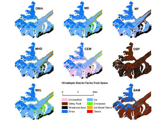
The OBIA method achieved the highest overall accuracy (Figure 10) for all glaciers, except G2. The average overall accuracy for all the five glaciers was found to be 87.33%. The average overall accuracy of the MHD yielded 78.67%. The MXL classifier outperformed the OBIA specifically for the G1 glacier (overall accuracy = 88.33%). However, when averaged over all the glaciers, it delivered an average of 78.71%. The MD classifier yielded an average overall accuracy of 72.81%. The CEM classifier delivered an average overall accuracy of 68.76%. The MF classifier provided an average overall accuracy of 58.48%. The OSP classifier yielded an overall accuracy at 32.00%. The SAM classifier was the poorest classifier among all the supervised classifiers, with an average overall accuracy of 30.48%. The average kappa statistic for each classifier for all the glaciers were also calculated along with the statistical error margin based on standard deviation to better ascertain the reliability of each classifier for such complex cryospheric applications (Figure 11).
The overall accuracy and the kappa statistic, coupled with the interpretations of the errors of commission and omission and the producer’s and user’s accuracy, were used to analyze each classifier with respect to the glacier in particular and the overall study area in general. Our results indicate that the OBIA method yielded the highest average kappa value (κ = 0.86), which testifies that it is the most reliable classification method in this study. The lowest deviation of the OBIA also indicates its potential for transferability to other regions. The MHD and MXL obtained a common average kappa value of 0.75. However, the MXL encompasses a higher margin of error than the MHD. The MD (κ = 0.72), CEM (κ = 0.63), MF (κ = 0.48), OSP (κ = 0.19), and SAM (κ = 0.17) have an orderly detrimental average kappa and high instability. Therefore, the trend of classifier reliability and accuracy is found to be OBIA > MHD > MXL > MD > CEM > MF > OSP > SAM (Figure 11). The results of each classification algorithm for every glacier are displayed in Figure 12, Figure 13, Figure 14, Figure 15 and Figure 16.
5. Discussion
5.1. Errors before Accuracies
It is common for studies reporting glacier classification results to present their evaluation based on either the overall accuracy, producer’s accuracy or the kappa statistic, such as that given by Shukla and Ali. [109], Ali et al. [3], and Bhardwaj et al. [36]. These studies also prefer using a “globally” accepted overall accuracy value of 85% for appreciable classification results. However, Congalton and Green [106] describe that this minimum acceptable standard is not true for every classification scheme across various applications. The “minimum” acceptable standard depends on the scene and the methods employed, in conjunction with the end-application. Foody [111] elaborates on the details concerning the origin and development of this “standard” and how it does not apply in every scenario. Nevertheless, both Congalton and Green [106] and Foody [111] maintain the robustness of the error matrix and its derivatives for evaluation of accuracy. Therefore, the results presented in Section 3 are broken down facies-wise with the assessment of over/underestimation as the primary evaluator. The overall accuracy and the kappa statistic are then utilized to gain a cumulative perspective of the results. It is furthermore common for studies to state the accuracy by comparing derived boundaries of glaciers against manually digitized or globally available digital boundaries [3,39,109]. However, we have used the manually digitized boundary (refer to Section 3.1) to extract the glacier from the surrounding terrain; this negates the probability of any form of confusion between debris classes and the surrounding valley.
The resultant classifier trends are in accordance with their applicability for each facies, rather than just on the overall accuracy. It is beyond the scope of this study to determine the algorithmic cause for the poor performance of the pixel classifiers, as this would require elaborations on the mathematical workings of each classifier. The evaluation presented here is to determine which algorithm/classifier/method performs better in the given scenario for each facies.
5.2. Comparative Analysis
As per our knowledge, the facies of the five selected glaciers of this study have not been mapped before. This makes close-quarter comparison a daunting task. However, Keshri et al. [33], Shukla et al. [90], Bhardwaj et al. [36], and Gupta et al. [112] have mapped glaciers within the same area and with approximately similar classes, hence a relatable evaluation of the results of this study is possible. Studies indicate that the most commonly used classifier for glacier classification is the MXL classifier [90,109,113,114]. Although it is traditionally employed for this purpose, hosts of other classifiers are available as of today. The efficacy of such a wide variety of classifiers has not been tested for mapping glacier surface facies. Given the importance of glacier facies, it is imperative to identify an extraction method which can be widely applied across glaciered regions. While most of the available research has reported facies like snow, ice, IMD, and debris [33,90,115], none have utilized the VNIR spectrum to extract crevasses. This study is the first of its kind to use OBIA on VHR VNIR imagery to isolate crevasses. In comparison to the PBIA approach, the OBIA successfully derived crevasses with 0% underestimation (Supplementary Table S3). SIR1 and SIR2 (Figure 2), combined with the areal constraints (Table 1) proved to be efficient at this task. While the SIRs may have identified crevasses through thresholding, precise segmentation permitted the successful mapping (Supplementary Figure S4). The MXL was the only supervised classifier to achieve comparable results. However, it underestimated crevasses by 21.11%, thus reducing its suitability.
Snow and ice are two of the most commonly classified facies/zonations on glaciers. Several studies have mapped snow and ice using the NDSI, NDGI, customized ratios, sensor-specific methodologies, and in situ spectra-based differentiation [4,18,24,32,33,108,112,116]. To that extent, even the OBIA approach has been tested [39,56]. Several degrees of accuracy have been achieved using a variety of methods for the mapping of snow and ice; however, we intend to explore the ability of our customized indices against the PBIA approach. In this study, the non-overlap of snow and ice spectra should provide suitable mapping for all the classifiers. However, it appears that while the OBIA and MHD approach achieved 100% accurate classification of snow, ice was more successfully extracted by the MXL. This could be in part due to the misclassification of ice pixels into crevasses by the OBIA, though this was limited to 20%. The advanced classifiers failed to map snow and ice with sufficient accuracy irrespective of the wide spectral differentiation. The reliability of the MXL in this regard supports even some of the earlier assertions of its effectivity [32]. Most Himalayan glaciers are said to be debris covered. While the mapping of debris-covered glaciers is a problem that has been approached from various angles, thermal data and/or elevation data seem to be the most widely adopted method [35,36,117]. Elevation is found to be useful even when coupled with Synthetic Aperture Radar SAR in an object-based domain [39]. The present imagery, being of early winter, consists of widespread ice and snow. This prohibits the strict definition of supraglacial and periglacial debris. Therefore, to solve this problem and to check the capacity for debris characterization in such a scenario, this study maps ice-mixed debris (IMD) and debris. IMD is reported in several glacier classification schemes [3,33,109,118,119] and is consistent with its separability from debris due to the mixing of snow (refer to Section 3.2.1 and Section 3.2.2). However, as the margin of differentiation between IMD and debris is low, their characterization is bound to consist of misclassifications. This stands true for all of the classifiers, including OBIA. The spectral overlap between IMD, debris, and shadowed areas in bands B1–B3 (Figure 5) led the OBIA protocol to generate complex objects within the shadowed region. It was initially assumed that this overlap would hinder the characterization of IMD and debris. However, SIR3 (Figure 2), which uses B2 over the mean of B7 and B8, was used to differentiate between IMD and debris. This was interesting, as the blue band (B2) falls in the middle of the overlap between IMD, debris, and shadowed area. This distinction appears to be due to the presence of ice, causing the spectral contrast between IMD and debris. While the OBIA performed better than the PBIA for extracting IMD, the MD was the best classifier of debris. This was a surprising result as it has underperformed for every other facies. This may point toward a prospective combination of SIR3 and MD for future characterization of debris classes. Due to the complex properties of objects generated within the shadowed areas, they were not effectively mapped using the SIRs and therefore the OBIA approach required manual digitization (refer to Section 3.3.2 and Figure 7). Hence, while the MXL proved to be the most reliable identifier of snow without any manual corrections, the OBIA achieved statistically better results due to the manual intervention. None of the advanced classifiers could map shadowed areas with significant accuracy.
Although the OBIA method achieved the maximum observable accuracy, it required ≈23 minutes for processing (Supplementary Table S4). The MXL, which is the best PBIA classifier of glacier facies in this study needed ≈14 minutes to perform classification, whereas the MHD required about 13.55 minutes to complete the classification. The MF method took the longest time to process the imagery, as it required an additional step of generating a MNF transform. Therefore, as far as the temporal constraint of each method is concerned, the MHD would be a better bargain if the accuracy need not be very high. This could be for cases when regional level mapping of facies is concerned. However, when the overall accuracy of the derived facies is the most important parameter, the OBIA should invariably be the method of choice.
5.3. Significances
Precipitation over the surface of a glacier is not limited to the accumulation zone; it is spread over the entire glacier. Although this imagery is of early winter, a large distribution of snow and ice is observed (Figure 4). This is indicative of a precipitation event and subsequent refreezing of snow over the surface of the glacier. However, even in such scenarios, the sporadic distribution of snow over the glacier tongue is rarely mapped by coarser resolution and conventional methods. The OBIA approach outlined in this study has successfully managed to map this distribution on the selected glaciers (Figure 12, Figure 13, Figure 14, Figure 15 and Figure 16). The FLAASH atmospheric correction played a key role not only in deriving spectral reflectance, but also in improving spectral separability (Supplementary Figures S2 and S3). Comparative studies of the FLAASH model [64,66] have found it to be comparable with the result of other models such as the Atmospheric Removal Program (ATREM), the Atmospheric Correction Now (ACORN), and the Quick Atmospheric Correction (QUAC). It offers an important feature for correcting light scattered from adjacent pixels into the field-of-view [120]. It is noted that when the input parameters of atmospheric correction are reliable and accurate, the FLAASH model provides more accurate results than faster methods such as the QUAC model [64]. In this study, all relevant input parameters are available (via imagery metadata) and as the atmospheric parameters could be assigned based on prior knowledge, the FLAASH model was selected for correcting atmospheric effects. Following the similarity of the extracted scaled spectral reflectance curve to Shukla et al. [90] and the criteria for differentiation between facies based on their reduced reflectance properties [40], this study identified the spectral properties of the observable facies across all five glaciers with relative ease. The resultant classification of the OBIA method is comparable to that of similar studies such as [33,90], who have identified similar classes in the same region. While the OBIA successfully extracted snow, crevasses, IMD, and shadowed areas, the PBIA-based MXL and MD performed better for ice and debris characterization. While the OBIA did not perform well for the ice and debris facies, it cannot be dismissed due to its effectivity in the separability of snow, crevasses, and IMD. Most studies depend on the usage of SWIR bands for facies and thermal data with elevation information for mapping debris classes [3,35,36,90,109,117]. However, we have mapped facies using only the VNIR spectrum. In this context, our results match the observation of Pope and Rees [4], who emphasize the use of VNIR wavelengths for mapping facies. Mapping of facies via any OBIA method ultimately depends upon the segmentation and the thresholds established. The thresholds in Table 1 are common for all five glaciers, except for the extraction of snow in glacier G2. While the thresholds may be common in this image due to similar sensing conditions for the entire imagery, the indices could potentially be transferable to other glaciers with scene-dependent threshold adjustments, a common observation over glaciers [118,121].
If we only compare the OBIA and PBIA approaches based on the errors and accuracies, it would appear that the OBIA approach is significantly better than the PBIA (Section 3 and Section 3.3). However, as it is elaborated in this study (Section 3), the complete picture is slightly different. Given the effectivity of the OBIA for snow, crevasses, and IMD, including manual digitization of boundaries and shadowed regions as well as the performance of the MXL and MD for ice and debris characterization, a synergistic combination could be an important future direction of research. Sahu and Gupta [122] propose such a merger of OBIA and PBIA methods for cryospheric applications. An effective methodology that combines the versatility of OBIA and the robustness of the PBIA could reduce the dependability of multiple kinds of ancillary inputs. Shukla and Yousuf [123] explain the necessity of ancillary inputs for the reduction of misclassification errors. However, this study has successfully mapped facies not only without multiple ancillary inputs, but also without dependence on SWIR bands. Therefore, rather than focusing on additional datasets, we propose the combination of our SIRs in an OBIA domain coupled with PBIA on VNIR spectrum datasets for the creation of a robust and transferable mechanism for mapping surface glacier facies.
5.4. Limitations
Saturation of snow in the VNIR spectrum is a recurring problem observed in similar studies. Pope and Rees [37] observed that even 16-bit Moderate Resolution Imaging Spectroradiometer (MODIS) data contained saturated snowy pixels. The WV-2 product used in this study is of 16-bit quantization; however, we have also observed saturated pixels in some parts of the snow facies. This is contributive to the characteristically high reflectance of snow observed in this study as well as by others [90]. Shadowed regions did not respond well to the indices and presented complex attributes (Figure 7) to both ice (when the shadows were lighter) and debris (when the shadows were much darker). Bhardwaj et al. [36] and Gore et al. [40] have observed similar problems in the shadowed regions. Gore et al. [40] points towards the use of higher radiometric resolution to solve this problem, however, our data is already 16-bit quantized. The non-availability of a higher radiometric product led to the use of manual digitization to identify and remove the shadowed area errors [36]. Although cumulatively the OBIA method was superior to the PBIA in terms of overall accuracy and the kappa statistic (refer to Section 3.3), it was more time-consuming and required consistent diligence. The PBIA, although less accurate, was far simpler in execution. Rastner et al. [56], who compared OBIA and PBIA for glacier mapping, have also found the limitation of time to be the most significant inhibitor in the usage of OBIA, a similar conclusion found in this study. Furthermore, the lack of any higher resolution imagery required that the same VNIR imagery be used for reference sample point generation. However, we followed the equalized random sampling approach based on Keshri et al. [33] and, as elaborated in Section 3.5, it was developed independently of the training sites used for the PBIA. The indices formed here are based on the spectral properties of WV-2. While it will be possible to test the indices on WV-2/3/4 imagery, inter-sensor transferability will not be easy. However, given the higher feature distinction capability and promising results with the WV-2 imagery, this study reiterates the importance and usefulness of sensor-specific indices for extracting maximum information from VHR multispectral data [124].
6. Conclusions
The present study tests the efficiency of OBIA and PBIA approaches for mapping surface glacier facies using VHR WorldView-2 imagery. Using a thorough preprocessing protocol to calibrate and correct the imagery for image analysis, subsets of five selected glaciers were extracted using manually digitized boundaries on a topographic reference. The OBIA approach permitted the coupling of segmentation and band ratioing to deliver three customized spectral index ratios that have the potential to be transferable across glaciered regions. While the OBIA approach achieved superior results for the identification of snow, crevasses, and IMD, the PBIA mapped ice and debris with the greatest accuracy. Shadowed regions were extracted manually via the OBIA, whereas the PBIA needed no such rectification. The differential capacities of the OBIA and PBIA techniques in mapping various facies have not been previously tested and no study has managed to map crevasses using the VNIR spectrum. One of the most important features of this study is its independence of SWIR bands and ancillary inputs. Among the seven classifiers tested of the PBIA approach, only MXL and MD managed to map ice and debris with high accuracies; no other classifier produced reasonable results. This study acknowledges its lack of field data for validation. However, the unbiased approach to sampling reference points highlights the strict validation performed. The focus on errors instead of accuracies scrutinizes every classifier for not only its overall performance, but also its performance for every thematic class. This heavily weighs down on the reliability of each method. The result concludes with the trend for overall classification accuracy and reliability as OBIA > MHD > MXL > MD > CEM > MF > OSP > SAM. However, as far as reliability is concerned facies-wise, the OBIA is successful for snow, crevasses, IMD, and even shadowed areas, whereas the PBIA is successful for ice and debris. While the OBIA approach is time-consuming and requires greater user intervention, the PBIA method is far less suitable for detailed feature mapping. Therefore, this study proposes a synergistic combination of OBIA and PBIA approaches to map surface glacier facies. Future research can focus on testing such a combined approach to provide detailed mapping of surface glacier facies, hence its transferability across varying scenarios and regions to fully realize their wide-ranging potential.
Supplementary Materials
The following are available online at https://www.mdpi.com/2072-4292/11/10/1207/s1.
Author Contributions
Conceptualization, S.D.J.; methodology and experimental design, S.D.J.; software and data processing, S.F.W. and S.D.J.; validation of results, S.D.J. and S.F.W.; formal analysis, S.F.W., supported by S.D.J.; investigation, S.D.J. and S.F.W.; resources, A.J.L. and S.D.J.; data curation, A.J.L.; writing—original draft preparation, S.F.W. and S.D.J.; writing—review and editing, S.D.J., S.F.W., and A.J.L.; visualization, S.F.W.; supervision, S.D.J. and A.J.L.; project administration, S.D.J. and A.J.L. The entire experiment, validation, manuscript preparation, and editing of the manuscript was conducted at the ESSO-NCPOR. The lead author (S.D.J) has recently moved to the SIOS, Longyearbyen, Norway.
Funding
This research received no external funding.
Acknowledgments
The authors thank the anonymous reviewers for their constructive comments, which helped improve the initial version of the manuscript. The authors also thank the editorial team at MDPI for their constant support throughout the processing of the manuscript. The authors thank Gangadhara Bhat, Chairman, Dept. of Geoinformatics, Mangalore University, and M. Ravichandran, Director ESSO-NCPOR for their motivation and support. This is NCPOR contribution J - 05/2019-20.
Conflicts of Interest
The authors declare no conflict of interest.
References
- Benson, C. Stratigraphic Studies in the Snow and Firn of the Greenland Ice Sheet, No. RR70; Cold Regions Research and Engineering Lab: Hanover NH, USA, 1962; Available online: http://acwc.sdp.sirsi.net/client/en_US/search/asset/1001392;jsessionid=351D596A6CE87F45BAEB04E7B9ECE897.enterprise-15000 (accessed on 17 January 2018).
- Paterson, W.S.B. The Physics of Glaciers, 3rd ed.; Pergamon: Oxford, UK, 1994. [Google Scholar]
- Ali, I.; Shukla, A.; Romshoo, S. Assessing linkages between spatial facies changes and dimensional variations of glaciers in the upper Indus Basin, western Himalaya. Geomorphology 2017, 284, 115–129. [Google Scholar] [CrossRef]
- Pope, A.; Rees, G. Using in situ spectra to explore Landsat classification of glacier surfaces. Int. J. Appl. Earth Obs. Geoinf. 2014, 27, 42–52. [Google Scholar] [CrossRef]
- Bamber, J.L.; Payne, A.J.; Houghton, J. Introduction and background. In Mass Balance of the Cryosphere: Observations and Modelling of Contemporary and Future Changes; Bamber, J.L., Payne, A.J., Eds.; Cambridge University Press: Cambridge, UK, 2004; pp. 1–8. [Google Scholar] [Green Version]
- Jiang, X.; Wang, N.; He, J.; Wu, X.; Song, G. A distributed surface energy and mass balance model and its application to a mountain glacier in China. Chin. Sci. Bull. 2010, 55, 2079–2087. [Google Scholar] [CrossRef]
- Paul, F.; Machguth, H.; Hoelzle, M.; Salzmann, N.; Haeberli, W. Alpinewide Distributed Glacier Mass Balance Modeling. In Darkening Peaks: Glacier Retreat, Science, and Society; Orlove, B., Wiegandt, E., Luckman, B., Eds.; University of California Press: Berkeley, CA, USA, 2008. [Google Scholar]
- Machguth, H.; Paul, F.; Hoelzle, M.; Haeberli, W. Distributed glacier mass-balance modelling as an important component of modern multi-level glacier monitoring. Ann. Glaciol. 2006, 43, 335–343. [Google Scholar] [CrossRef] [Green Version]
- Schuler, T.; Hock, R.; Jackson, M.; Elvehøy, H.; Braun, M.; Brown, I.; Hagen, J. Distributed mass-balance and climate sensitivity modelling of Engabreen, Norway. Ann. Glaciol. 2005, 42, 395–401. [Google Scholar] [CrossRef] [Green Version]
- Braun, M.; Hock, R. Spatially distributed surface energy balance and ablation modelling on the ice cap of King George Island (Antarctica). Glob. Planet. Chang. 2004, 42, 45–58. [Google Scholar] [CrossRef]
- Mölg, T.; Hardy, D. Ablation and associated energy balance of a horizontal glacier surface on Kilimanjaro. J. Geophys. Res. 2004, 109, D16104. [Google Scholar] [CrossRef]
- (Lisette) Klok, E.; Oerlemans, J. Model study of the spatial distribution of the energy and mass balance of Morteratschgletscher, Switzerland. J. Glaciol. 2002, 48, 505–518. [Google Scholar] [CrossRef] [Green Version]
- Blard, P.; Wagnon, P.; Lavé, J.; Soruco, A.; Sicart, J.; Francou, B. Degree-day melt models for paleoclimate reconstruction from tropical glaciers: Calibration from mass balance and meteorological data of the Zongo glacier (Bolivia, 16° S). Clim. Past Discuss. 2011, 7, 2119–2158. [Google Scholar] [CrossRef]
- Huintjes, E.; Li, H.; Sauter, T.; Li, Z.; Schneider, C. Degree-day modelling of the surface mass balance of Urumqi Glacier No. 1, Tian Shan, China. Cryosphere Discuss. 2010, 4, 207–232. [Google Scholar] [CrossRef] [Green Version]
- Jóhannesson, T.; Sigurdsson, O.; Laumann, T.; Kennett, M. Degree-day glacier mass-balance modelling with applications to glaciers in Iceland, Norway and Greenland. J. Glaciol. 1995, 41, 345–358. [Google Scholar] [CrossRef] [Green Version]
- Braithwaite, R. Positive degree-day factors for ablation on the Greenland ice sheet studied by energy-balance modelling. J. Glaciol. 1995, 41, 153–160. [Google Scholar] [CrossRef] [Green Version]
- Braun, M.; Schuler, T.V.; Hock, R.; Brown, I.; Jackson, M. Comparison of remote sensing derived glacier facies maps with distributed mass balance modelling at Engabreen, northern Norway. IAHS Publ. Ser. Proc. Rep. 2007, 318, 126–134. [Google Scholar]
- Paul, F.; Winsvold, S.; Kääb, A.; Nagler, T.; Schwaizer, G. Glacier Remote Sensing Using Sentinel-2. Part II: Mapping Glacier Extents and Surface Facies, and Comparison to Landsat 8. Remote Sens. 2016, 8, 575. [Google Scholar] [CrossRef]
- Winsvold, S.; Kaab, A.; Nuth, C. Regional Glacier Mapping Using Optical Satellite Data Time Series. IEEE J. Sel. Top. Appl. Earth Obs. Remote Sens. 2016, 9, 3698–3711. [Google Scholar] [CrossRef] [Green Version]
- Nolin, A.; Payne, M. Classification of glacier zones in western Greenland using albedo and surface roughness from the Multi-angle Imaging SpectroRadiometer (MISR). Remote Sens. Environ. 2007, 107, 264–275. [Google Scholar] [CrossRef]
- Heiskanen, J.; Kajuutti, K.; Jackson, M.; Elvehøy, H.; Pellikka, P. Assessment of glaciological parameters using landsat sat-ellite data in svartisen, northern norway. In Proceedings of the EARSeL-LISSIG-Workshop Observing our Cryosphere from Space, Bern, Switzerland, 11–13 March 2002; Volume 35. [Google Scholar]
- Williams, R.; Hall, D.; Benson, C. Analysis of glacier facies using satellite techniques. J. Glaciol. 1991, 37, 120–128. [Google Scholar] [CrossRef] [Green Version]
- Hall, D.; Chang, A.; Siddalingaiah, H. Reflectances of glaciers as calculated using Landsat-5 Thematic Mapper data. Remote Sens. Environ. 1988, 25, 311–321. [Google Scholar] [CrossRef]
- Hall, D.; Ormsby, J.; Bindschadler, R.; Siddalingaiah, H. Characterization of Snow and Ice Reflectance Zones on Glaciers Using Landsat Thematic Mapper Data. Ann. Glaciol. 1987, 9, 104–108. [Google Scholar] [CrossRef]
- Huang, L.; Li, Z.; Tian, B.; Chen, Q.; Liu, J.; Zhang, R. Classification and snow line detection for glacial areas using the polarimetric SAR image. Remote Sens. Environ. 2011, 115, 1721–1732. [Google Scholar] [CrossRef]
- Arigony-Neto, J.; Saurer, H.; Simões, J.; Rau, F.; Jaña, R.; Vogt, S.; Gossmann, H. Spatial and temporal changes in dry-snow line altitude on the Antarctic Peninsula. Clim. Chang. 2009, 94, 19–33. [Google Scholar]
- Brown, I.A. Radar facies on the West Greenland ice sheet: Comparison with AVHRR albedo data. In Geoinformation for European-Wide Integration, Proceedings of the 22nd Symposium of the European Association of Remote Sensing Laboratories, Prague, Czech Republic, 4–6 June 2002; Benes, T., Ed.; Millpress: Rotterdam, The Netherlands.
- Engeset, R.; Kohler, J.; Melvold, K.; Lundén, B. Change detection and monitoring of glacier mass balance and facies using ERS SAR winter images over Svalbard. Int. J. Remote Sens. 2002, 23, 2023–2050. [Google Scholar] [CrossRef]
- Braun, M.; Rau, F. Using a multi-year data archive of ERS SAR imagery for the monitoring of firn line positions and ablation patterns on the King George Island ice cap (Antarctica). In Proceedings of the SIG-Workshop Land Ice and Snow, Dresden, Germany, 16–17 June 2000; Volume 1, pp. 281–291. [Google Scholar]
- Braun, M.; Rau, F.; Saurer, H.; Gobmann, H. Development of radar glacier zones on the King George Island ice cap, Antarctica, during austral summer 1996/97 as observed in ERS-2 SAR data. Ann. Glaciol. 2000, 31, 357–363. [Google Scholar] [CrossRef] [Green Version]
- Partington, K. Discrimination of glacier facies using multi-temporal SAR data. J. Glaciol. 1998, 44, 42–53. [Google Scholar] [CrossRef] [Green Version]
- Sidjak, R.W. Glacier mapping of the Illecillewaet icefield, British Columbia, Canada, using Landsat TM and digital elevation data. Int. J. Remote Sens. 1999, 20, 273–284. [Google Scholar] [CrossRef]
- Keshri, A.; Shukla, A.; Gupta, R. ASTER ratio indices for supraglacial terrain mapping. Int. J. Remote Sens. 2009, 30, 519–524. [Google Scholar] [CrossRef]
- Shukla, A.; Arora, M.; Gupta, R. Synergistic approach for mapping debris-covered glaciers using optical–thermal remote sensing data with inputs from geomorphometric parameters. Remote Sens. Environ. 2010, 114, 1378–1387. [Google Scholar] [CrossRef]
- Racoviteanu, A.; Williams, M. Decision Tree and Texture Analysis for Mapping Debris-Covered Glaciers in the Kangchenjunga Area, Eastern Himalaya. Remote Sens. 2012, 4, 3078–3109. [Google Scholar] [CrossRef] [Green Version]
- Bhardwaj, A.; Joshi, P.; Snehmani; Singh, M.; Sam, L.; Gupta, R. Mapping debris-covered glaciers and identifying factors affecting the accuracy. Cold Reg. Sci. Technol. 2014, 106–107, 161–174. [Google Scholar] [CrossRef]
- Pope, A.; Rees, W. Impact of spatial, spectral, and radiometric properties of multispectral imagers on glacier surface classification. Remote Sens. Environ. 2014, 141, 1–13. [Google Scholar] [CrossRef]
- Kundu, S.; Chakraborty, M. Delineation of glacial zones of Gangotri and other glaciers of Central Himalaya using RISAT-1 C-band dual-pol SAR. Int. J. Remote Sens. 2015, 36, 1529–1550. [Google Scholar] [CrossRef]
- Robson, B.; Nuth, C.; Dahl, S.; Hölbling, D.; Strozzi, T.; Nielsen, P. Automated classification of debris-covered glaciers combining optical, SAR and topographic data in an object-based environment. Remote Sens. Environ. 2015, 170, 372–387. [Google Scholar] [CrossRef] [Green Version]
- Gore, A.; Mani, S.; Shekhar, C.; Ganju, A. Glacier surface characteristics derivation and monitoring using Hyperspectral datasets: A case study of Gepang Gath glacier, Western Himalaya. Geocarto Int. 2017, 34, 23–42. [Google Scholar] [CrossRef]
- Lillesand, T.; Kiefer, R.W.; Chipman, J. Remote Sensing and Image Interpretation; John Wiley & Sons: Hoboken, NJ, USA, 2014. [Google Scholar]
- Richards, J.A. Remote Sensing Digital Image Analysis; Springer: Berlin/Heidelberg, Germany, 2013. [Google Scholar]
- Fisher, P. The pixel: A snare and a delusion. Int. J. Remote Sens. 1997, 18, 679–685. [Google Scholar] [CrossRef]
- Wei, W.; Chen, X.; Ma, A. Object-oriented information extraction and application in high-resolution remote sensing image. In Proceedings of the IEEE Geoscience and Remote Sensing Symposium, Seoul, Korea, 29 July 2005; Volume 6, pp. 3803–3806. [Google Scholar]
- Jensen, J.R.; Lulla, K. Introductory digital image processing: A remote sensing perspective. Geocarto Int. 1987, 2, 65. [Google Scholar] [CrossRef]
- Price, J. How unique are spectral signatures? Remote Sens. Environ. 1994, 49, 181–186. [Google Scholar] [CrossRef]
- Blaschke, T. Object based image analysis for remote sensing. ISPRS J. Photogramm. Remote Sens. 2010, 65, 2–16. [Google Scholar] [CrossRef] [Green Version]
- Li, M.; Zang, S.; Zhang, B.; Li, S.; Wu, C. A Review of Remote Sensing Image Classification Techniques: The Role of Spatio-contextual Information. Eur. J. Remote Sens. 2014, 47, 389–411. [Google Scholar] [CrossRef]
- Arbiol, R.; Zhang, Y.; i Comellas, V.P. Advanced classification techniques: A review. Rev. Catalana Geogr. 2007, 12, 31. Available online: https://www.raco.cat/index.php/RCG/article/view/79653/103912 (accessed on 29 January 2018).
- Liu, D.; Xia, F. Assessing object-based classification: Advantages and limitations. Remote Sens. Lett. 2010, 1, 187–194. [Google Scholar] [CrossRef]
- Weih, R.C.; Riggan, N.D. Object-based classification vs. pixel-based classification: Comparative importance of multi-resolution imagery. Int. Arch. Photogram. Remote Sens. Spat. Inf. Sci. 2010, 38, C7. [Google Scholar]
- Gao, Y.; Mas, J.F. A comparison of the performance of pixel-based and object-based classifications over images with various spatial resolutions. Online J. Earth Sci. 2008, 2, 27–35. [Google Scholar]
- Jawak, S.; Wankhede, S.; Luis, A. Exploration of Glacier Surface Facies Mapping Techniques Using Very High Resolution Worldview-2 Satellite Data. Proceedings 2018, 2, 339. [Google Scholar] [CrossRef]
- Jawak, S.; Wankhede, S.; Luis, A. Comparison of pixel and object-based classification techniques for glacier facies extraction. ISPRS Int. Arch. Photogram. Remote Sens. Spat. Inf. Sci. 2018, XLII-5, 543–548. [Google Scholar] [CrossRef]
- Jawak, S.D.; Wankhede, S.F.; Luis, A.J. Prospective of high resolution worldview-2 satellite data for geospatial surface facies mapping of an alpine glacier. In Proceedings of the Asian Conference on Remote Sensing 2017, New Delhi, India, 23–27 October 2017; Available online: https://a-a-r-s.org/proceeding/ACRS2017/ID_5_749/177.pdf (accessed on 2 February 2018).
- Rastner, P.; Bolch, T.; Notarnicola, C.; Paul, F. A Comparison of Pixel- and Object-Based Glacier Classification with Optical Satellite Images. IEEE J. Sel. Top. Appl. Earth Obs. Remote Sens. 2014, 7, 853–862. [Google Scholar] [CrossRef]
- Paul, F.; Hendricks, J. Optical remote sensing of glacier extent. In Remote Sensing of Glaciers: Techniques for Topographic, Spatial and Thematic Mapping of Glaciers; Taylor & Francis Group: Boca Raton, Fl, USA, 2010; pp. 137–152. [Google Scholar]
- Shaw, G.A.; Burke, H.K. Spectral imaging for remote sensing. Linc. Lab. J. 2003, 14, 3–28. [Google Scholar]
- Du, Y.; Teillet, P.; Cihlar, J. Radiometric normalization of multitemporal high-resolution satellite images with quality control for land cover change detection. Remote Sens. Environ. 2002, 82, 123–134. [Google Scholar] [CrossRef]
- Jawak, S.D.; Luis, A.J. Geospatial mapping of Antarctic coastal oasis using geographic object-based image analysis and high resolution satellite imagery. In Multispectral, Hyperspectral, and Ultraspectral Remote Sensing Technology, Techniques and Applications VI, Proceedings of International Society for Optics and Photonics 2016; SPIE: Asia-Pacific Remote Sensing, New Delhi, India, 2016; Volume 9880, p. 98801Q. [Google Scholar]
- Zhang, Z.; He, G.; Zhang, X.; Long, T.; Wang, G.; Wang, M. A coupled atmospheric and topographic correction algorithm for remotely sensed satellite imagery over mountainous terrain. Gisci. Remote Sens. 2017, 55, 400–416. [Google Scholar] [CrossRef]
- Hadjit, H.; Oukebdane, A.; Belbachir, A. Atmospheric correction of Earth-observation remote sensing images by Monte Carlo method. J. Earth Syst. Sci. 2013, 122, 1219–1235. [Google Scholar] [CrossRef] [Green Version]
- Module, F.L.A.A.S.H. Atmospheric correction module: Quac and flaash user’s guide. Version 2009, 4, 44. [Google Scholar]
- Guo, Y.; Zeng, F. Atmospheric Correction Comparison of Spot-5 image based on model flaash and model quac. ISPRS Int. Arch. Photogram. Remote Sens. Spat. Inf. Sci. 2012, XXXIX-B7, 7–11. [Google Scholar] [CrossRef]
- Yuan, J.; Niu, Z. Evaluation of atmospheric correction using FLAASH. In Proceedings of the 2008 International Workshop on Earth Observation and Remote Sensing Applications 2008, Beijing, China, 30 June–2 July 2008; pp. 1–6. [Google Scholar]
- Kruse, F.A. Comparison of ATREM, ACORN, and FLAASH atmospheric corrections using low-altitude AVIRIS data of Boulder, CO. In Proceedings of the Summaries of 13th JPL Airborne Geoscience Workshop 2004, Jet Propulsion Lab, Pasadena, CA, USA, 31 March–2 April 2004. [Google Scholar]
- Felde, G.W.; Anderson, G.P.; Cooley, T.W.; Matthew, M.W.; Berk, A.; Lee, J. Analysis of Hyperion data with the FLAASH atmospheric correction algorithm. In Proceedings of the IEEE Geoscience and Remote Sensing Symposium, Toulouse, France, 21–25 July 2003; Volume 1, pp. 90–92. [Google Scholar]
- Cooley, T.; Anderson, G.P.; Felde, G.W.; Hoke, M.L.; Ratkowski, A.J.; Chetwynd, J.H.; Gardner, J.A.; Adler-Golden, S.M.; Matthew, M.W.; Berk, A.; et al. FLAASH, a MODTRAN4-based atmospheric correction algorithm, its application and validation. In Proceedings of the Geoscience and Remote Sensing Symposium, Toronto, ON, Canada, 24–28 July 2002; Volume 3, pp. 1414–1418. [Google Scholar]
- Pope, E.; Willis, I.; Pope, A.; Miles, E.; Arnold, N.; Rees, W. Contrasting snow and ice albedos derived from MODIS, Landsat ETM+ and airborne data from Langjökull, Iceland. Remote Sens. Environ. 2016, 175, 183–195. [Google Scholar] [CrossRef]
- Jawak, S.; Luis, A. A spectral index ratio-based Antarctic land-cover mapping using hyperspatial 8-band WorldView-2 imagery. Pol. Sci. 2013, 7, 18–38. [Google Scholar] [CrossRef] [Green Version]
- Jawak, S.; Luis, A. Improved land cover mapping using high resolution multiangle 8-band WorldView-2 satellite remote sensing data. J. Appl. Remote Sens. 2013, 7, 073573. [Google Scholar] [CrossRef]
- Jawak, S.D.; Khopkar, P.S.; Jadhav, S.P.; Luis, A.J. Customization of Normalized Difference of Snow Index (NDSI) for extraction of snow and/or ice cover from cryospheric surface using WorldView-2 data. In Proceedings of the International Conference on Geospatial Momentum for Society & Environment: AGSE 2013, Ahmedabad, India, 16–19 December 2013. [Google Scholar]
- Jawak, S.D.; Luis, A.J. Applications of WorldView-2 satellite data for extraction of polar spatial information and DEM of Larsemann Hills, East Antarctica. In Proceedings of the International Conference on Fuzzy Systems and Neural Computing 2011, Hong Kong, China, 20–21 February 2011; Volume 3, p. 978-1. [Google Scholar]
- Jawak, S.D.; Luis, A.J. High Resolution 8-Band WorldView-2 Satellite Remote Sensing Data for Polar Geospatial Information Mining and Thematic Elevation Mapping of Larsemann Hills, East Antarctica. In Proceedings of the 11th ISAES 2011, Edinburgh, Scotland, 10–16 July 2011. [Google Scholar]
- Aguilar, M.; Saldaña, M.; Aguilar, F. GeoEye-1 and WorldView-2 pan-sharpened imagery for object-based classification in urban environments. Int. J. Remote Sens. 2013, 34, 2583–2606. [Google Scholar] [CrossRef]
- Mausel, P.W.; Kramber, W.J.; Lee, J.K. Optimum band selection for supervised classification of multispectral data. Photogramm. Eng. Remote Sens. 1990, 56, 55–60. [Google Scholar]
- Cracknell, A.P.; Hayes, L. Introduction to Remote Sensing; Taylor & Francis: New York, NY, USA, 1991. [Google Scholar]
- Song, C.; Woodcock, C.; Seto, K.; Lenney, M.; Macomber, S. Classification and Change Detection Using Landsat TM Data. Remote Sens. Environ. 2001, 75, 230–244. [Google Scholar] [CrossRef]
- Rott, H. Thematic studies in alpine areas by means of polarimetric SAR and optical imagery. Adv. Space Res. 1994, 14, 217–226. [Google Scholar] [CrossRef]
- Nolin, A.; Dozier, J.; Mertes, L. Mapping alpine snow using a spectral mixture modeling technique. Ann. Glaciol. 1993, 17, 121–124. [Google Scholar] [CrossRef] [Green Version]
- Matthew, M.W.; Adler-Golden, S.M.; Berk, A.; Felde, G.; Anderson, G.P.; Gorodetzky, D.; Paswaters, S.; Shippert, M. Atmospheric correction of spectral imagery: Evaluation of the FLAASH algorithm with AVIRIS data. In Proceedings of the IEEE Applied Imagery Pattern Recognition Workshop 2002, Washington, DC, USA, 16–18 October 2002; pp. 157–163. [Google Scholar]
- Perkins, T.; Adler-Golden, S.; Cappelaere, P.; Mandl, D. High-speed atmospheric correction for spectral image processing. In Algorithms and Technologies for Multispectral, Hyperspectral, and Ultraspectral Remote Sensing Technology, Techniques and Applications VI, Proceedings of International Society for Optics and Photonics 2012; SPIE: Bellingham, WA, USA, 2012; Volume 8390, p. 83900V. [Google Scholar]
- Kaufman, Y.; Wald, A.; Remer, L.; Gao, B.-C.; Li, R.-R.; Flynn, L. The MODIS 2.1-μm channel-correlation with visible reflectance for use in remote sensing of aerosol. IEEE Trans. Geosci. Remote Sens. 1997, 35, 1286–1298. [Google Scholar] [CrossRef]
- Harrisgeospatial.com. Available online: https://www.harrisgeospatial.com/docs/backgroundflaash.html (accessed on 21 June 2018).
- Abreu, L.W.; Anderson, G.P. The MODTRAN 2/3 report and LOWTRAN 7 model. Contract 1996, 19628, 0132. [Google Scholar]
- Kpalma, K.; El-Mezouar, M.C.; Taleb, N. Recent trends in satellite image pan-sharpening techniques. In Proceedings of the 1st International Conference on Electrical, Electronic and Computing Engineering, Vrnjačka Banja, Serbia, 2–5 June 2014. [Google Scholar]
- Laben, C.A.; Brower, B.V. Process for Enhancing the Spatial Resolution of Multispectral Imagery Using Pan-Sharpening. U.S. Patent 6,011,875, 4 January 2000. [Google Scholar]
- Maurer, T. How to pan-sharpen images using the gram-schmidt pan-sharpen method—A recipe. ISPRS Int. Arch. Photogramm. Remote Sens. Spat. Inf. Sci. 2013, XL-1/W1, 239–244. [Google Scholar] [CrossRef]
- Raup, B.H.; Andreassen, L.M.; Bolch, T.; Bevan, S. Remote sensing of glaciers. In Remote Sensing of the Cryosphere, 1st ed.; Tedesco, M., Ed.; John Wiley & Sons: Hoboken, NJ, USA, 2014; pp. 123–156. [Google Scholar]
- Shukla, A.; Gupta, R.; Arora, M. Estimation of debris cover and its temporal variation using optical satellite sensor data: A case study in Chenab basin, Himalaya. J. Glaciol. 2009, 55, 444–452. [Google Scholar] [CrossRef]
- Tempfli, K.; Huurneman, G.C.; Bakker, W.H.; Janssen, L.L.F.; Feringa, W.F.; Gieske, A.S.M.; Grabmaier, K.A.; Hecker, C.A.; van der Horn, J.A. Principles of Remote Sensing: An introductory Textbook; ITC: Enschede, The Netherlands, 2009. [Google Scholar]
- Baatz, M.; Schape, A. Multiresolution Segmentation: An Optimization Approach for High Quality Multi-Scale Image Segmentation. In Angewandte Geographische Informations-Verarbeitung XII; Strobl, J., Blaschke, T., Griesbner, G., Eds.; Wichmann Verlag: Karlsruhe, Germany, 2000; pp. 12–23. [Google Scholar]
- Pellikka, P.; Rees, G. Remote Sensing of Glaciers; CRC Press: Boca Raton, FL, USA, 2010. [Google Scholar]
- Dozier, J.; Painter, T. Multispectral and hyperspectral remote sensing of alpine snow properties. Annu. Rev. Earth Planet. Sci. 2004, 32, 465–494. [Google Scholar] [CrossRef]
- Definiens Developer 7. Reference Book; Definiens AG: Munich, Germany, 2007. [Google Scholar]
- Rott, H.; Markl, G. Improved snow and glacier monitoring by the Landsat Thematic Mapper. In Proceedings of the Workshop on the Landsat Thematic Mapper Applications, ESA SP-1102, Frascati, Italy, December 1989; pp. 3–12. Available online: https://www.researchgate.net/publication/292541417_Improved_snow_and_glacier_monitoring_by_the_Landsat_Thematic_Mapper (accessed on 12 December 2018).
- Bronge, L.; Bronge, C. Ice and snow-type classification in the Vestfold Hills, East Antarctica, using Landsat-TM data and ground radiometer measurements. Int. J. Remote Sens. 1999, 20, 225–240. [Google Scholar] [CrossRef]
- Dozier, J. Spectral signature of alpine snow cover from the landsat thematic mapper. Remote Sens. Environ. 1989, 28, 9–22. [Google Scholar] [CrossRef]
- Xiao, X.; Shen, Z.; Qin, X. Assessing the potential of VEGETATION sensor data for mapping snow and ice cover: A Normalized Difference Snow and Ice Index. Int. J. Remote Sens. 2001, 22, 2479–2487. [Google Scholar] [CrossRef]
- Shimamura, Y.; Izumi, T.; Matsuyama, H. Evaluation of a useful method to identify snow-covered areas under vegetation—Comparisons among a newly proposed snow index, normalized difference snow index, and visible reflectance. Int. J. Remote Sens. 2006, 27, 4867–4884. [Google Scholar] [CrossRef]
- Kruse, F.A. Geologic mapping using combined analysis of Airborne Visible/Infrared Imaging Spectrometer (AVIRIS) and SIR-C/X-SAR data. In Imaging Spectrometry II. Proc. SPIE 1996, 2819, 24–36. [Google Scholar]
- Boardman, J.W.; Kruse, F.A. Automated spectral analysis: A geological example using AVIRIS data, north Grapevine Mountains, Nevada. In Proceedings of the ERIM Tenth Thematic Conference on Geologic Remote Sensing, Environmental Research Institute of Michigan 1994, San Antonio, TX, USA, 9–12 May 1994; pp. I-407–I-418. [Google Scholar]
- Green, A.; Berman, M.; Switzer, P.; Craig, M. A transformation for ordering multispectral data in terms of image quality with implications for noise removal. IEEE Trans. Geosci. Remote Sens. 1988, 26, 65–74. [Google Scholar] [CrossRef] [Green Version]
- Jensen, R.R.; Shumway, J.M. Sampling Our World. In Research Methods in Geography; Gomez, B., Jones, J.P., III, Eds.; Wiley Blackwell: New York, NY, USA, 2010; pp. 77–90. [Google Scholar]
- Foody, G. Assessing the accuracy of land cover change with imperfect ground reference data. Remote Sens. Environ. 2010, 114, 2271–2285. [Google Scholar] [CrossRef] [Green Version]
- Congalton, R.; Green, K. Assessing the Accuracy of Remotely Sensed Data: Principles and Practices; CRC Press: Boca Raton, FL, USA, 2009. [Google Scholar]
- Negi, H.S.; Shekhar, C.; Singh, S.K. Snow and glacier investigations using hyperspectral data in the Himalaya. Curr. Sci. 2015, 10, 892–902. [Google Scholar]
- König, M.; Winther, J.; Isaksson, E. Measuring snow and glacier ice properties from satellite. Rev. Geophys. 2001, 39, 1–27. [Google Scholar] [CrossRef]
- Shukla, A.; Ali, I. A hierarchical knowledge-based classification for glacier terrain mapping: A case study from Kolahoi Glacier, Kashmir Himalaya. Ann. Glaciol. 2016, 57, 1–10. [Google Scholar] [CrossRef]
- Foody, G.; Mathur, A. A relative evaluation of multiclass image classification by support vector machines. IEEE Trans. Geosci. Remote Sens. 2004, 42, 1335–1343. [Google Scholar] [CrossRef] [Green Version]
- Foody, G. Harshness in image classification accuracy assessment. Int. J. Remote Sens. 2008, 29, 3137–3158. [Google Scholar] [CrossRef] [Green Version]
- Gupta, R.; Haritashya, U.; Singh, P. Mapping dry/wet snow cover in the Indian Himalayas using IRS multispectral imagery. Remote Sens. Environ. 2005, 97, 458–469. [Google Scholar] [CrossRef]
- Karimi, N.; Farokhnia, A.; Karimi, L.; Eftekhari, M.; Ghalkhani, H. Combining optical and thermal remote sensing data for mapping debris-covered glaciers (Alamkouh Glaciers, Iran). Cold Reg. Sci. Technol. 2012, 71, 73–83. [Google Scholar] [CrossRef]
- Khan, A.; Naz, B.; Bowling, L. Separating snow, clean and debris covered ice in the Upper Indus Basin, Hindukush-Karakoram-Himalayas, using Landsat images between 1998 and 2002. J. Hydrol. 2015, 521, 46–64. [Google Scholar] [CrossRef] [Green Version]
- Ghosh, S.; Pandey, A.; Nathawat, M. Mapping of debris-covered glaciers in parts of the Greater Himalaya Range, Ladakh, western Himalaya, using remote sensing and GIS. J. Appl. Remote Sens. 2014, 8, 083579. [Google Scholar] [CrossRef]
- Kulkarni, A.; Rathore, B.; Singh, S. Ajai Distribution of seasonal snow cover in central and western Himalaya. Ann. Glaciol. 2010, 51, 123–128. [Google Scholar] [CrossRef]
- Bhambri, R.; Bolch, T.; Chaujar, R. Mapping of debris-covered glaciers in the Garhwal Himalayas using ASTER DEMs and thermal data. Int. J. Remote Sens. 2011, 32, 8095–8119. [Google Scholar] [CrossRef] [Green Version]
- Bhardwaj, A.; Joshi, P.; Snehmani; Sam, L.; Singh, M.; Singh, S.; Kumar, R. Applicability of Landsat 8 data for characterizing glacier facies and supraglacial debris. Int. J. Appl. Earth Obs. Geoinf. 2015, 38, 51–64. [Google Scholar] [CrossRef]
- Zhang, J.; Jia, L.; Menenti, M.; Hu, G. Glacier Facies Mapping Using a Machine-Learning Algorithm: The Parlung Zangbo Basin Case Study. Remote Sens. 2019, 11, 452. [Google Scholar] [CrossRef]
- Gao, B.; Montes, M.; Davis, C.; Goetz, A. Atmospheric correction algorithms for hyperspectral remote sensing data of land and ocean. Remote Sens. Environ. 2009, 113, S17–S24. [Google Scholar] [CrossRef]
- Alifu, H.; Johnson, B.; Tateishi, R. Delineation of Debris-Covered Glaciers Based on a Combination of Geomorphometric Parameters and a TIR/NIR/SWIR Band Ratio. IEEE J. Sel. Top. Appl. Earth Obs. Remote Sens. 2016, 9, 781–792. [Google Scholar] [CrossRef]
- Sahu, R.; Gupta, R.D. Conceptual framework of combined pixel and object-based method for delineation of debris-covered glaciers. ISPRS Ann. Photogramm. Remote Sens. Spatial Inf. Sci. 2018, IV-5, 173–180. [Google Scholar] [CrossRef]
- Shukla, A.; Yousuf, B. Evaluation of multisource data for glacier terrain mapping: A neural net approach. Geocarto Int. 2016, 32, 569–587. [Google Scholar] [CrossRef]
- Casey, K.; Kääb, A.; Benn, D. Geochemical characterization of supraglacial debris via in situ and optical remote sensing methods: A case study in Khumbu Himalaya, Nepal. Cryosphere 2012, 6, 85–100. [Google Scholar] [CrossRef]
Figure 1.
Geographic location of the study area on the WorldView-2 imagery (obtained via DigitalGlobe). The boundary of each glacier is highlighted in red. The RGB band combination is given by Red: Band 8; Green: Band 4; and Blue: Band 3. The bottom left inset shows the location of the entire study area within the Indian subcontinent. The boundaries of glaciers G1 and G5 lie at the border of the image extent.

Figure 2.
Calibration and preprocessing of the WorldView-2 (WV-2) imagery. The Advanced Spaceborne Thermal Emission and Reflection (ASTER) Global digital Elevation Model (GDEM) was used to generate the 3-dimensional (3D) surface for delineating the glacier boundary. The three spectral index ratios (SIRs) developed for mapping facies in the object based image analysis (OBIA) protocol are depicted as SIR 1, SIR 2 and SIR 3 respectively. The pixel based image analysis (PBIA) approach performed on the extracted study area and is performed independently of the OBIA protocol.

Figure 3.
Utilization of Advanced Spaceborne Thermal Emission and Reflection (ASTER) Global digital Elevation Model (GDEM) v2 in conjunction with the WV-2 image for delineation of glacial boundaries. (a) Cirque without digitized boundary, (b) ice divides with digitized boundary, (c) 3-dimensional surface showing digitized boundary coincides with snow line on the cirque wall.

Figure 4.
Visual distinctions between each of the observable surface facies. The numbered red boundaries demark the example sites for each facies. The band combination used here is Red: Band 5; Green: Band 3; and Blue: Band 2. The scale for each zoomed-in box (numbered 1–6) is according to the scale needed to identify the target facies.

Figure 5.
Average scaled spectral reflectance plots of the various surface facies observed in this study. The values used to generate this plot are averaged across each of the five glaciers tested in this study. The spectral bands listed in the y-axis are B1: Coastal; B2: Blue; B3: Green; B4: Yellow; B5: Red; B6: Red edge; B7: Near infrared 1 (NIR-1); and B8: Near infrared 2 (NIR-2).

Figure 6.
Customized spectral indices and their resultant outputs. The resultant outputs are displayed for the G5 glacier.
Figure 6.
Customized spectral indices and their resultant outputs. The resultant outputs are displayed for the G5 glacier.

Figure 7.
Spectral variations within a shadow region as highlighted by SIR1, SIR2, and SIR3.
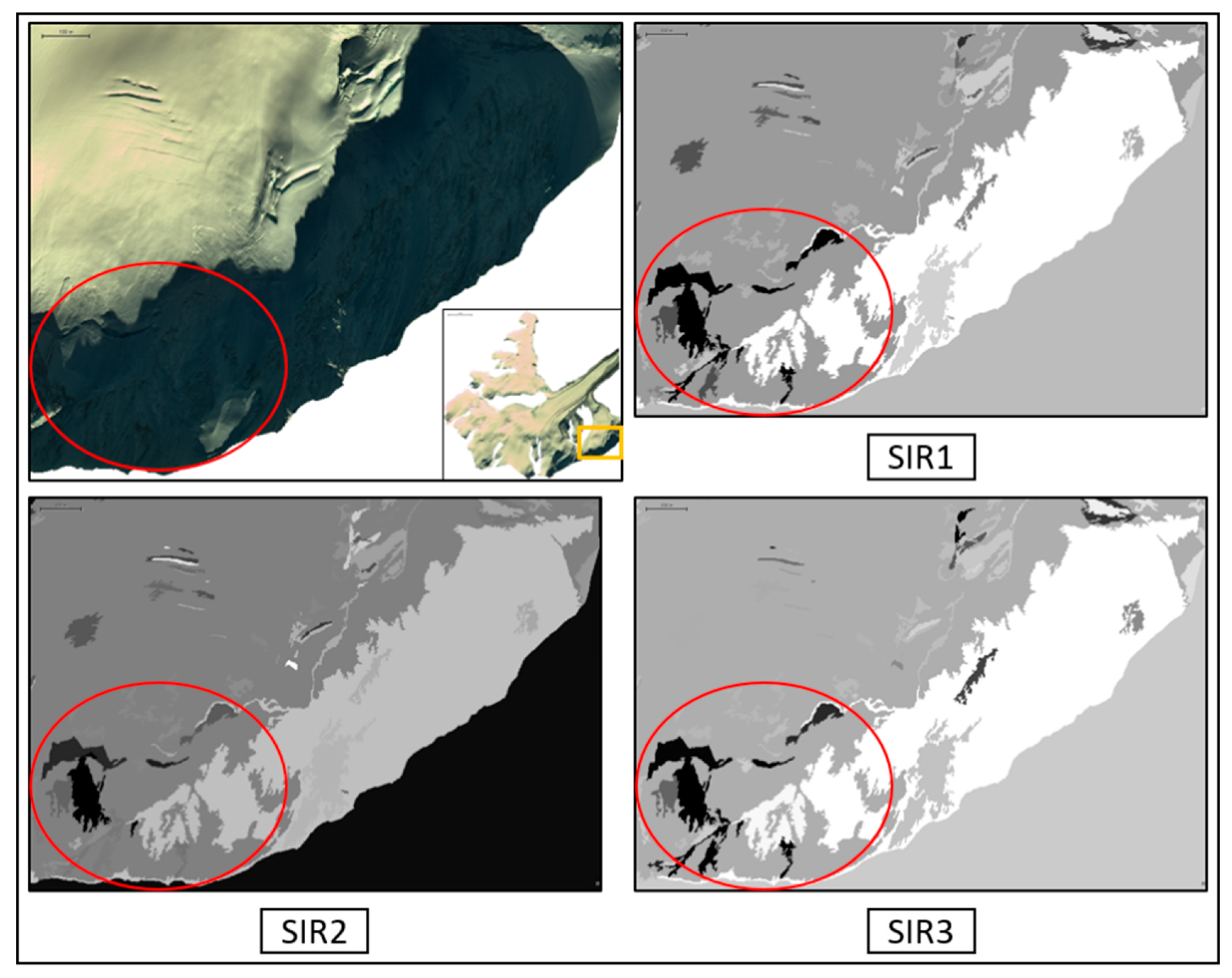
Figure 8.
Allocation of training sites defined for the conventional and advanced pixel classifiers. Training sites are defined for each of the glaciers, G1 (upper left), G2 (center left), G3 (upper right), G4 (center right), G5 (lower left).
Figure 8.
Allocation of training sites defined for the conventional and advanced pixel classifiers. Training sites are defined for each of the glaciers, G1 (upper left), G2 (center left), G3 (upper right), G4 (center right), G5 (lower left).

Figure 9.
Distribution of reference sample points per glacier; G1 (upper left), G2 (center left), G3 (upper right), G4 (center right), and G5 (lower left).
Figure 9.
Distribution of reference sample points per glacier; G1 (upper left), G2 (center left), G3 (upper right), G4 (center right), and G5 (lower left).
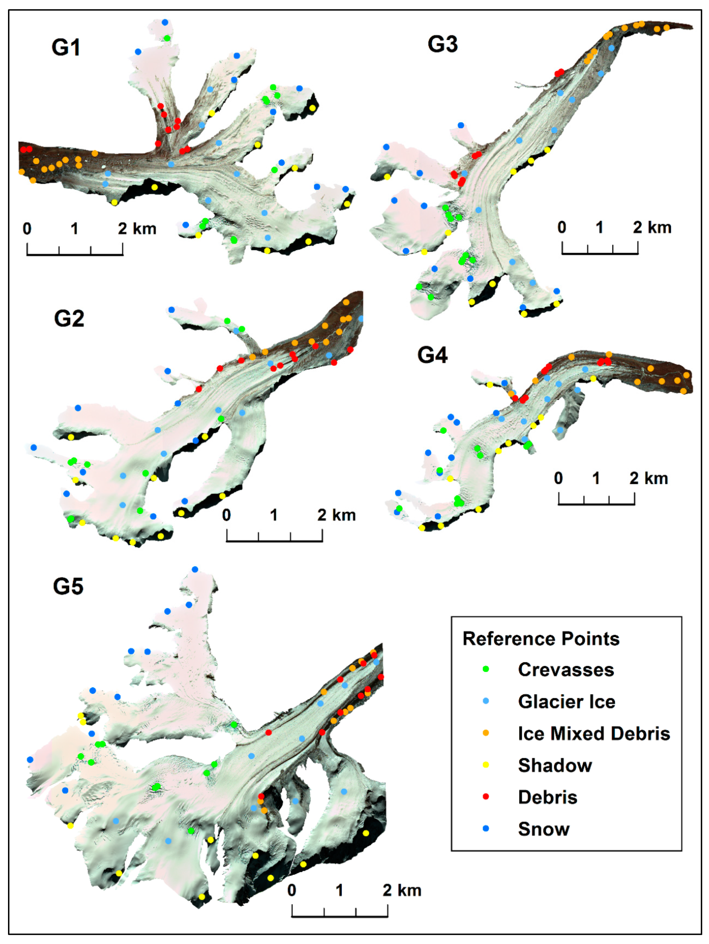
Figure 10.
Scatter plot of the overall accuracy (%) of each classifier for each glacier. The plot can be interpreted as a trend analysis of the performance of each classifier as per the overall accuracy for each glacier. OBIA: Object Based Image Analysis; MHD: Mahalanobis Distance; MXL: Maximum Likelihood; MD: Minimum Distance; CEM: Constrained Energy Minimization; MF: Matched Filtering; OSP: Orthogonal Space Projection; SAM: Spectral Angle Mapper.
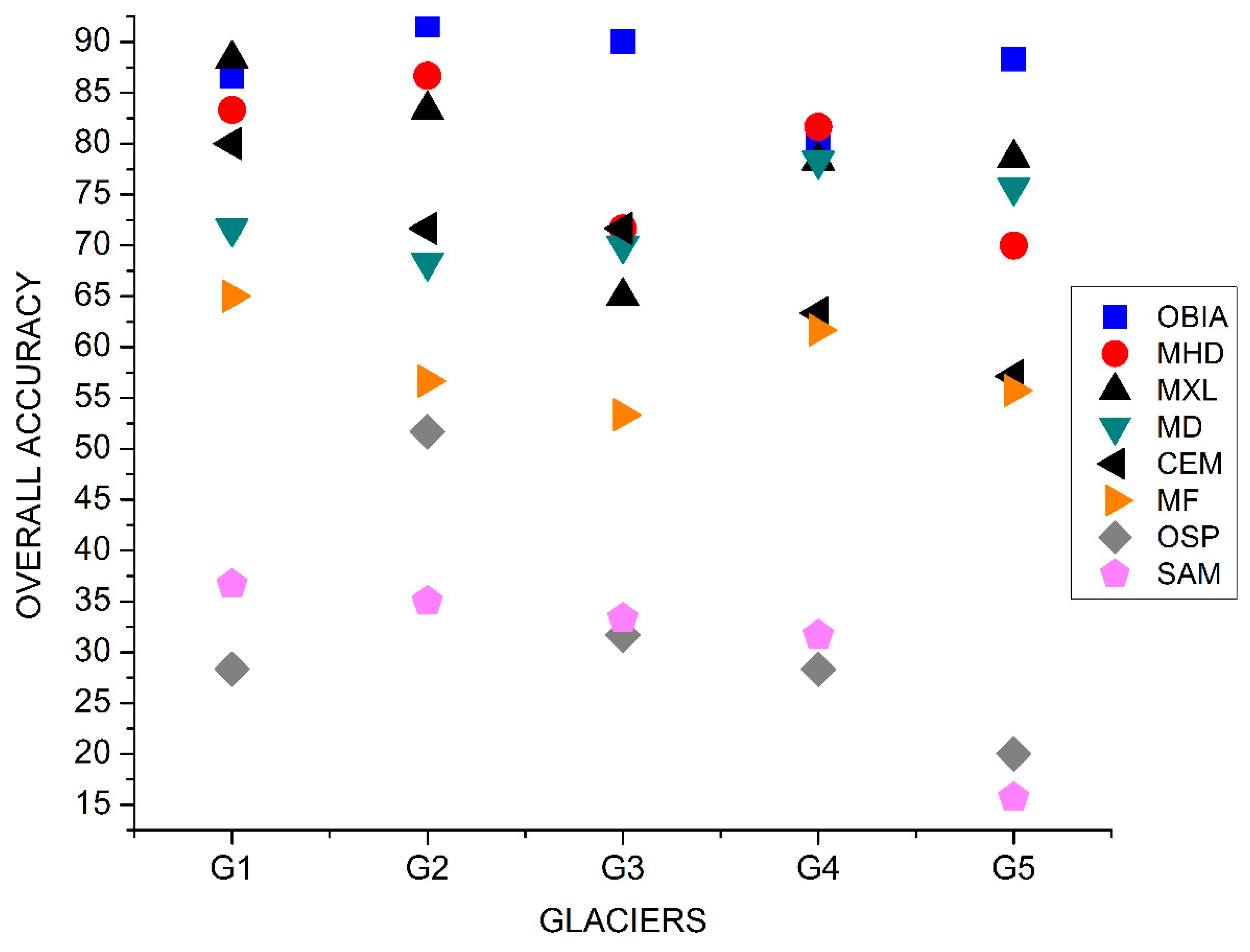
Figure 11.
Average kappa statistic for the entire study region with error margins for each classifier.
Figure 11.
Average kappa statistic for the entire study region with error margins for each classifier.
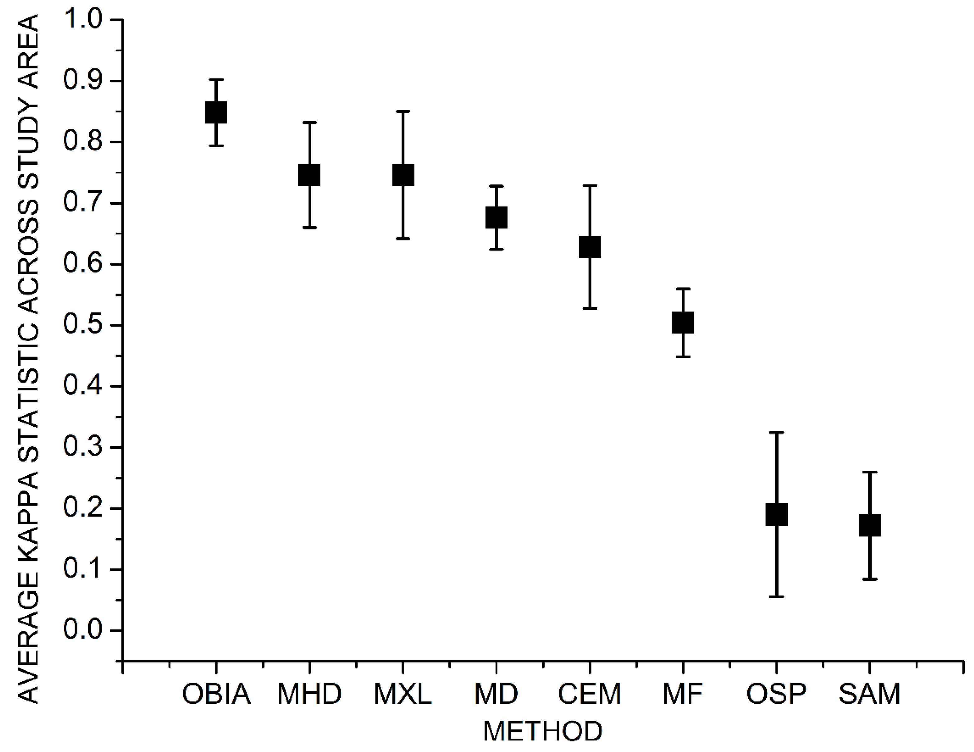
Figure 12.
Thematic classification results of glacier G1
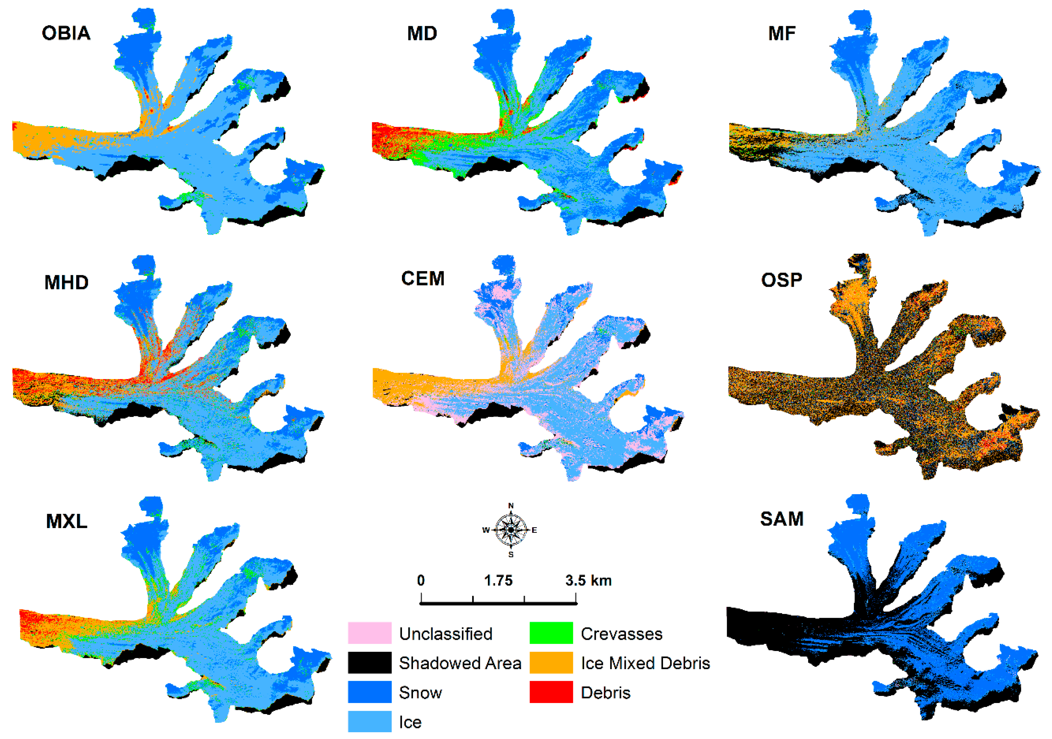
Figure 13.
Thematic classification results of glacier G2.
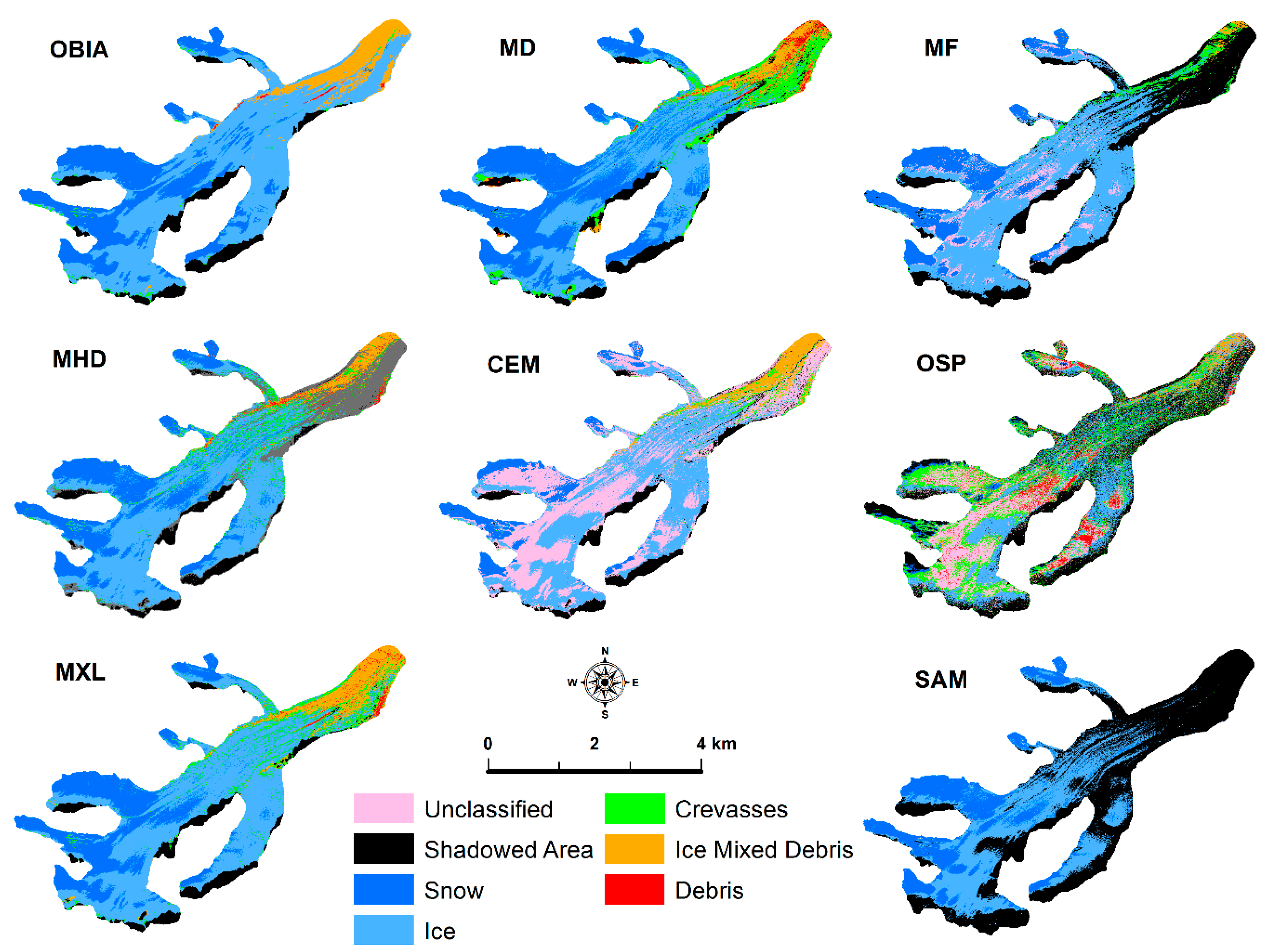
Figure 14.
Thematic classification results of glacier G3.
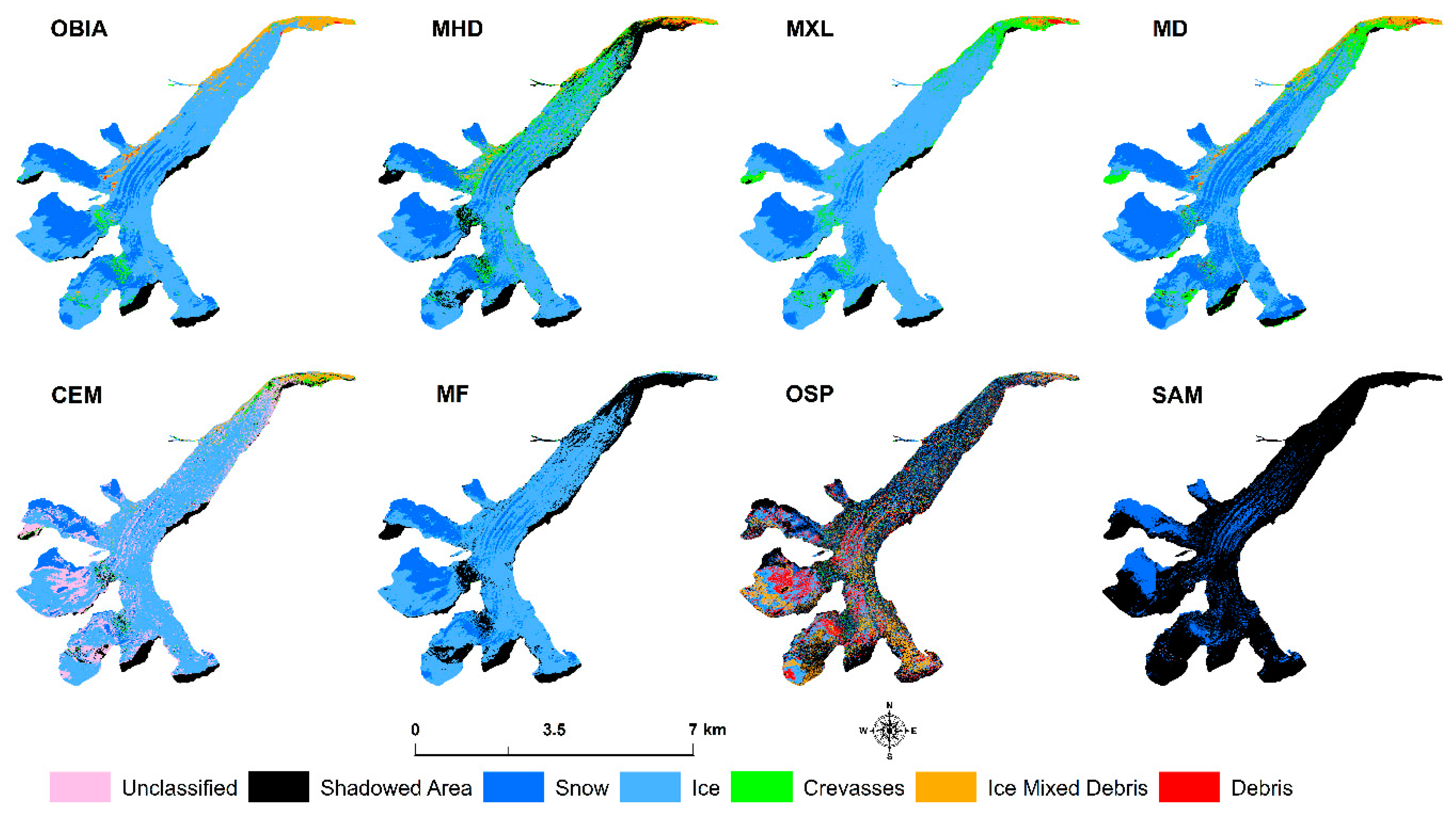
Figure 15.
Thematic classification results of glacier G4.

Figure 16.
Thematic classification results of G5.
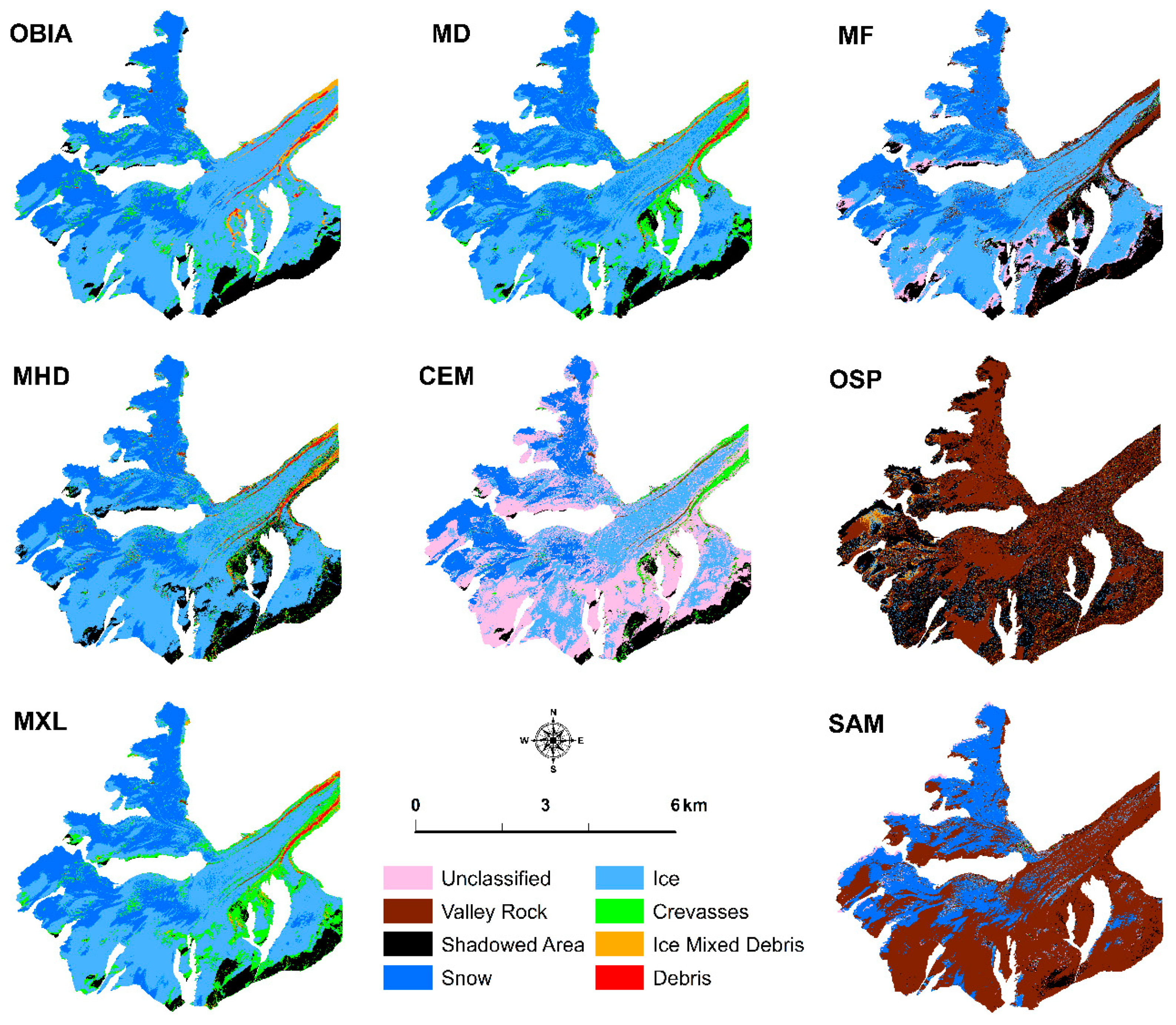

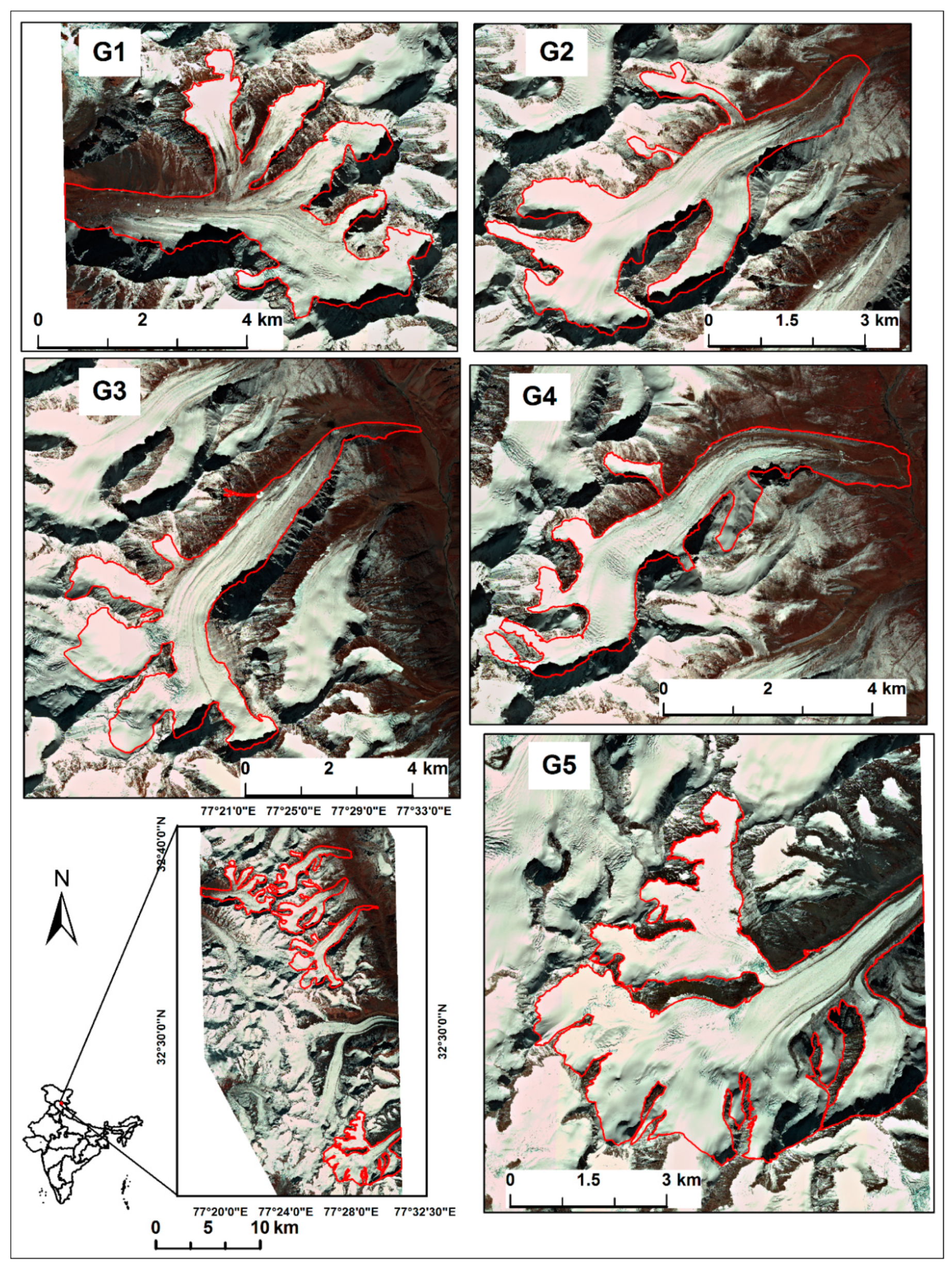
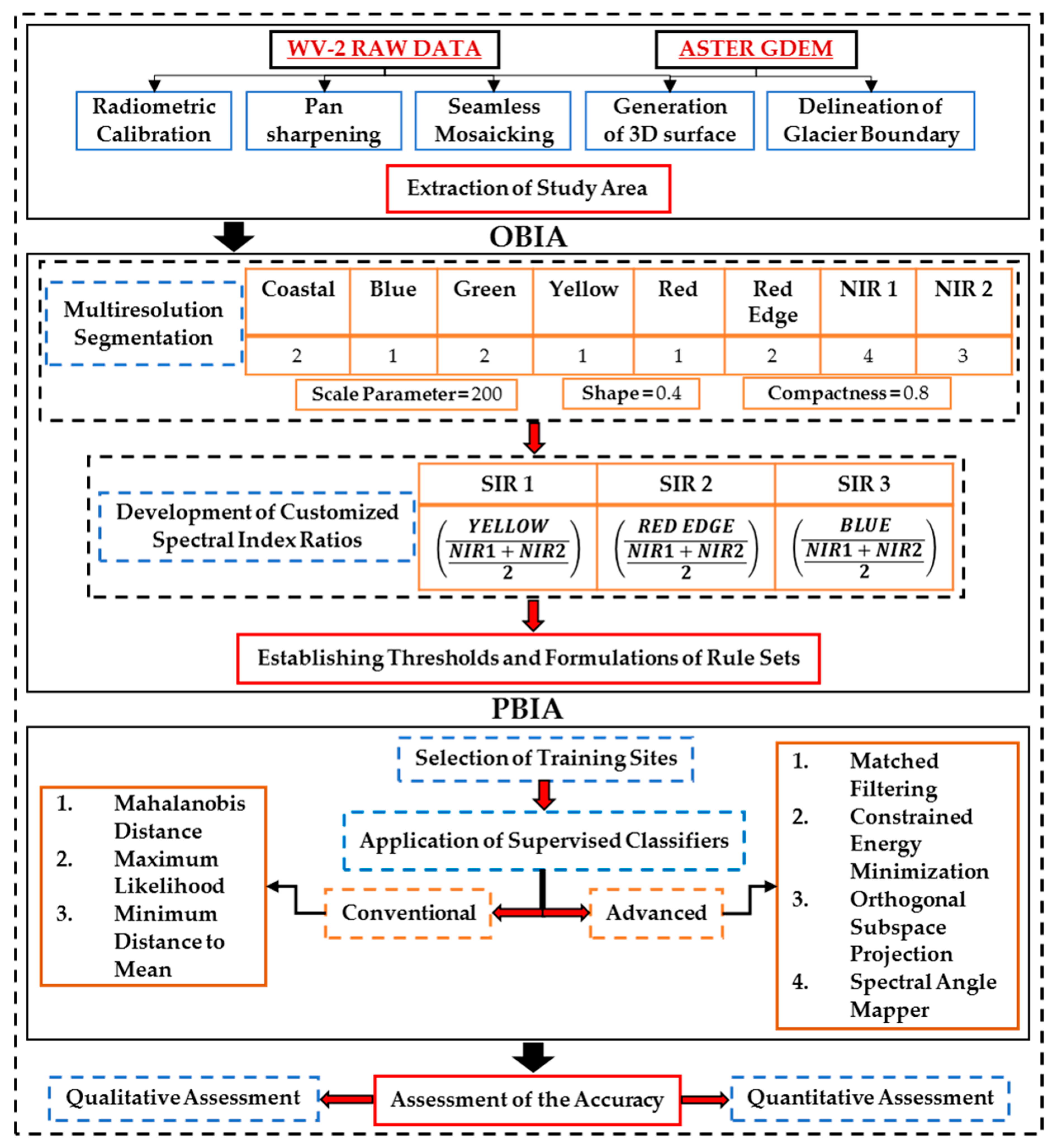
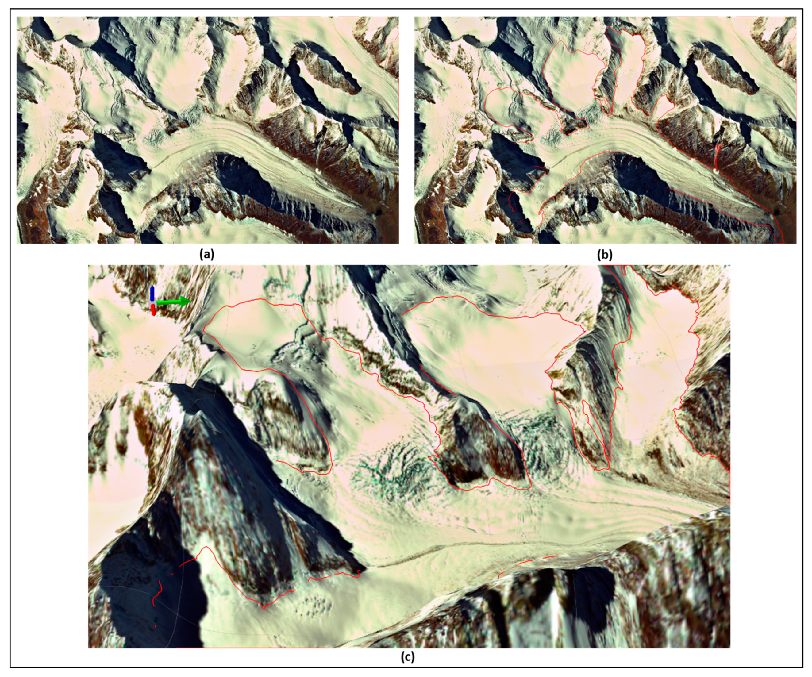
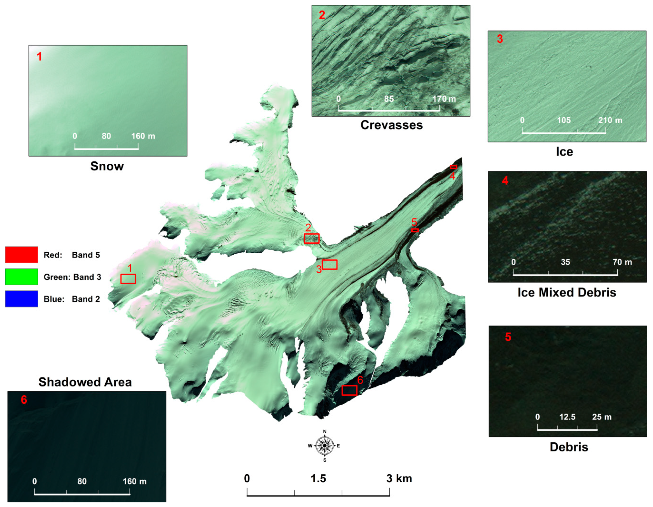
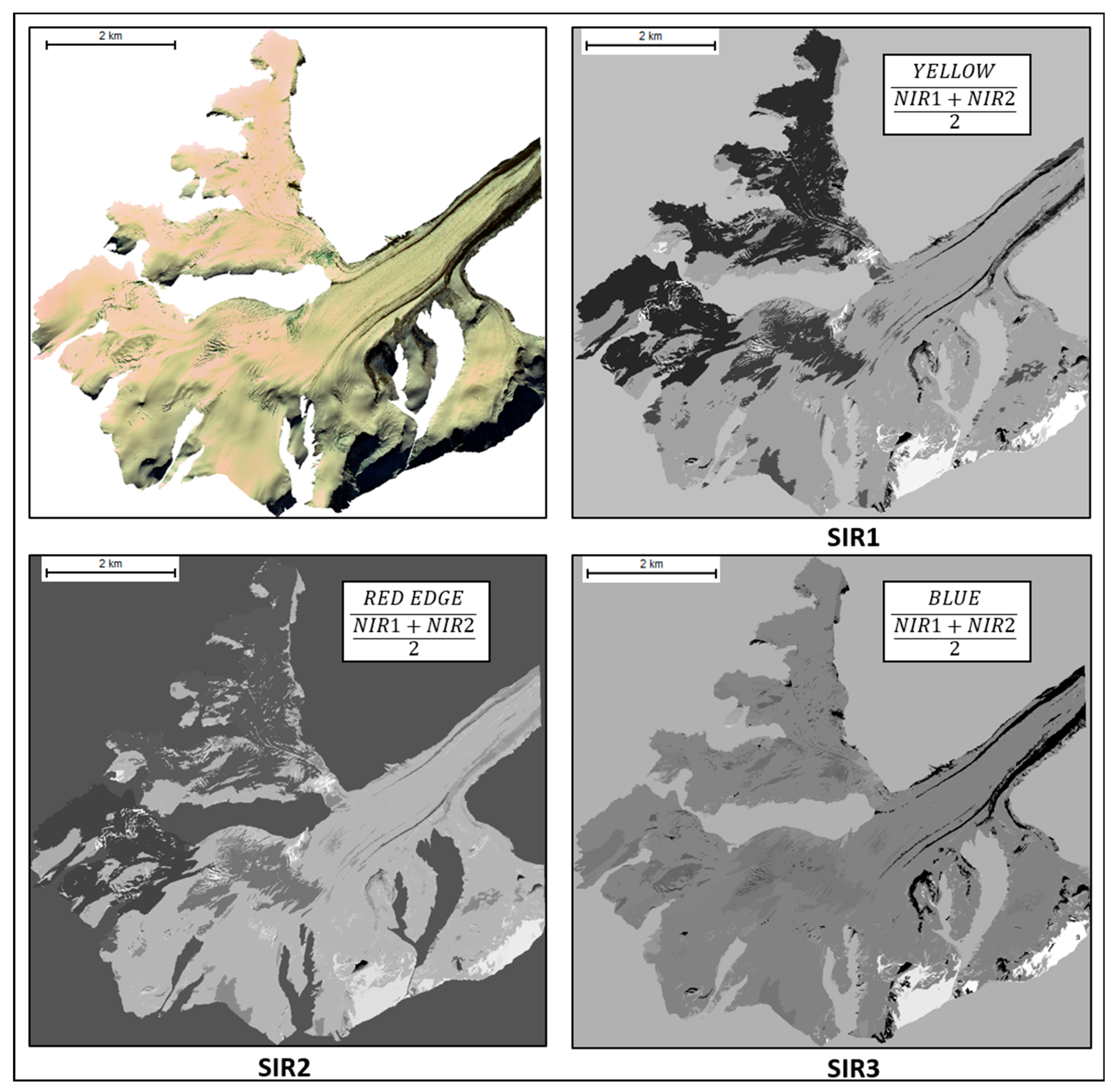
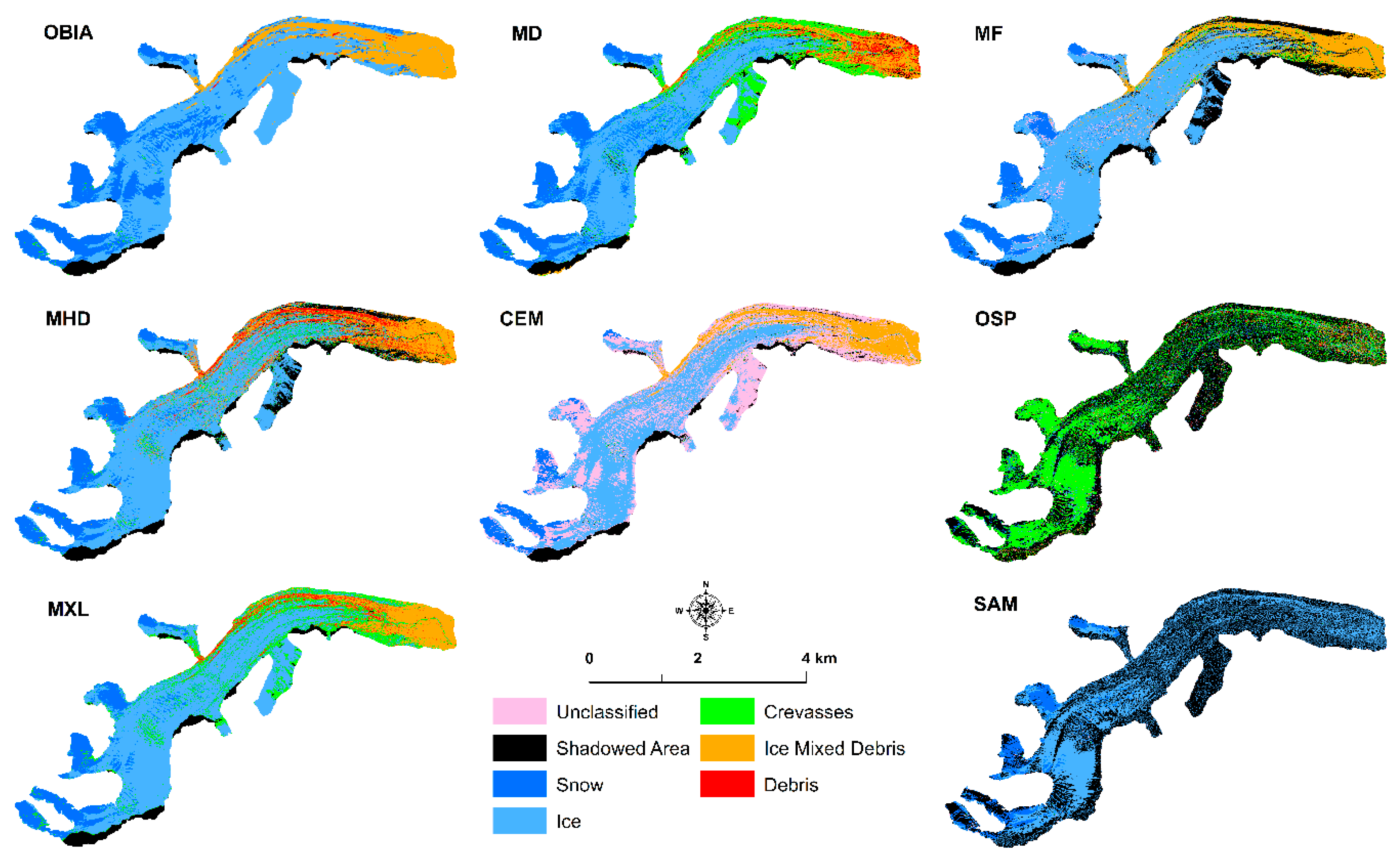
Table 1.
Thresholds established for classifying the selected glaciers. The index-wise thresholds and contextual parameters for each thematic class were common, except for glacier G2 where the classification of snow required only a threshold of <0.7 for spectral index ratio 2 (SIR2).
Table 1.
Thresholds established for classifying the selected glaciers. The index-wise thresholds and contextual parameters for each thematic class were common, except for glacier G2 where the classification of snow required only a threshold of <0.7 for spectral index ratio 2 (SIR2).
| Thematic Class | Index-Wise Threshold | Glaciers | Contextual Parameter |
|---|---|---|---|
| Snow | SIR2 < 0.7 | G2 | |
| SIR2 < 0.74 | G1, G3, G4, G5 | ||
| SIR2 < 0.75 | Relative border to snow > 0.3 | ||
| Ice | SIR1 < 0.63 | G1, G2 G3, G4, G5 | |
| SIR1 < 0.7 and SIR2 < 0.79 | |||
| SIR1 < 0.68 and SIR2 < 0.8 | |||
| Debris | SIR3 < 0 | ||
| SIR3 < 0.1 | |||
| Ice-Mixed Debris | SIR3 < 0.35 | ||
| SIR3 ≤ 0.455 | |||
| Crevasses | SIR1 > 0.7 | ||
| SIR1 > 0.65 | Area < 400 pixel | ||
| SIR1 > 0.65 | Area = 300 pixel | ||
| SIR1 < 0.67 and SIR2 < 0.8 |
Table 2.
The stretch and rule threshold applied to each of the advanced classifiers.
| Classifier | Stretch | Rule Threshold |
|---|---|---|
| MF | Square Root | 0.400 |
| CEM | Square Root | 0.800 |
| SAM | Square Root | 0.600 |
| OSP | Square Root | 0.700 |
© 2019 by the authors. Licensee MDPI, Basel, Switzerland. This article is an open access article distributed under the terms and conditions of the Creative Commons Attribution (CC BY) license (http://creativecommons.org/licenses/by/4.0/).
Share and Cite
MDPI and ACS Style
Jawak, S.D.; Wankhede, S.F.; Luis, A.J. Explorative Study on Mapping Surface Facies of Selected Glaciers from Chandra Basin, Himalaya Using WorldView-2 Data. Remote Sens. 2019, 11, 1207. https://doi.org/10.3390/rs11101207
AMA Style
Jawak SD, Wankhede SF, Luis AJ. Explorative Study on Mapping Surface Facies of Selected Glaciers from Chandra Basin, Himalaya Using WorldView-2 Data. Remote Sensing. 2019; 11(10):1207. https://doi.org/10.3390/rs11101207
Chicago/Turabian StyleJawak, Shridhar D., Sagar F. Wankhede, and Alvarinho J. Luis. 2019. "Explorative Study on Mapping Surface Facies of Selected Glaciers from Chandra Basin, Himalaya Using WorldView-2 Data" Remote Sensing 11, no. 10: 1207. https://doi.org/10.3390/rs11101207
Note that from the first issue of 2016, this journal uses article numbers instead of page numbers. See further details here.