Analysis of Vegetation Red Edge with Different Illuminated/Shaded Canopy Proportions and to Construct Normalized Difference Canopy Shadow Index

Abstract

Shadows exist universally in sunlight-source remotely sensed images, and can interfere with the spectral morphological features of green vegetations, resulting in imprecise mathematical algorithms for vegetation monitoring and physiological diagnoses; therefore, research on shadows resulting from forest canopy internal composition is very important. Red edge is an ideal indicator for green vegetation’s photosynthesis and biomass because of its strong connection with physicochemical parameters. In this study, red edge parameters (curve slope and reflectance) and the normalized difference vegetation index (NDVI) of two species of coniferous trees in Inner Mongolia, China, were studied using an unmanned aerial vehicle’s hyperspectral visible-to-near-infrared images. Positive correlations between vegetation red edge slope and reflectance with different illuminated/shaded canopy proportions were obtained, with all R²s beyond 0.850 (p < 0.01). NDVI values performed steadily under changes of canopy shadow proportions. Therefore, we devised a new vegetation index named normalized difference canopy shadow index (NDCSI) using red edge’s reflectance and the NDVI. Positive correlations (R² = 0.886, p < 0.01) between measured brightness values and NDCSI of validation samples indicated that NDCSI could differentiate illumination/shadow circumstances of a vegetation canopy quantitatively. Combined with the bare soil index (BSI), NDCSI was applied for linear spectral mixture analysis (LSMA) using Sentinel-2 multispectral imaging. Positive correlations (R² = 0.827, p < 0.01) between measured brightness values and fractional illuminated vegetation cover (FIVC) demonstrate the capacity of NDCSI to accurately calculate the fractional cover of illuminated/shaded vegetation, which can be utilized to calculate and extract the illuminated vegetation canopy from satellite images.

1. Introduction

Vegetation is an important component of the global ecosystem that can ameliorate climate change and maintain the global carbon cycle [1]. Remote sensing technology is suited for investigating vegetation distribution and studying its biological characteristics frequently and inexpensively [2]. However, coniferous forests have complex canopy structures through which sunlight can be refracted and reflected repeatedly, causing shadows in remote sensing images [3,4]. Vegetation shadows are caused generally by sunlight being blocked by topographic relief or canopy obscuration, causing energy loss and the darkening of vision in remotely sensed images [5,6]. Shadows reduce the spectral information of vegetation and interfere with tree species classification, biomass calculation, and quantitative algorithm construction [7,8,9]. Also, the amount of leaves exposed to sunlight is closely related to the intensity of photosynthesis, which is an important pathway for energy exchange and atmosphere adjustment [10,11,12]. The vegetation spectral shape affected by sunlight reflectance ranges mainly from the visible to the near-infrared bands, causing large differences in spectral curves of the same vegetation species [13,14]. With the development of spectroscopy technology, the image quality and spatial resolution of sensors are improving constantly [15,16]. The ability for images to display the details of the target has been improved, while the shadow details have been enhanced as well. For this reason, the interference of shadows on image pixels is also increasing with finer spatial resolutions [17]. How to effectively detect and quantify the shadow proportion in satellite imagery has become a subject of much research.

Shadows have been found to have considerable negative effects on remotely sensed images [18]. To prevent the adverse effects of shadows on images, most of the research concerned shadow monitoring, shadow recognition and removal [19]. In [20] by Sinclair, the vegetation canopy was considered into sunlit or shaded leaves to propose the simplified soil-plant-atmosphere model, and photosynthesis was calculated. The related model has been continuously developed and modified, for example, by Mercado and Sprintsin [21,22]. Mercado modified the JULES land-surface scheme and took into account variations in direct and diffuse radiation on sunlit and shaded canopy photosynthesis. Sprintsin modeled gross primary productivity using two-leaf (separating the canopy into sunlit and shaded parts) and big-leaf upscaling approaches. A model of bidirectional reflectance for forests was proposed by Strahler [23] in a comprehensive consideration of sunlit canopy, shaded canopy, sunlit background, and shaded background. Two simple physical models of vegetation reflectance have been derived to correct satellite imagery for bidirectional and topographic effects by Dymond [24]. Pu has developed a stepwise masking system to separate sunlit and shaded image-objects of tree canopies to aid in forest species mapping [25]. Researchers have studied the influence of shadows on vegetation and have proposed models for quantitative retrieval of fractional vegetation cover [26,27,28,29]. Four-Scale geometric optical modeling was promoted by J M Chen based on Li-Strahler and describes the aggregation effect between canopies or among the leaves [30,31,32,33]. It fully takes into account different spatial scales and further refines canopy structure characteristics. Results of above-mentioned studies have indicated the importance of an accurate description of canopy structure and its shadow conditions.

Former studies and their proposed models have considered the impact resulting from canopy shadows, but mainly at the scale of a single tree. Complex parameters and higher-order functions were usually included in the models to explain physical processes and to analyze photon mechanisms between leaves, such as scattering, reflection and absorption. These models are sufficient for theoretical analysis of vegetation shadows and for drawing conclusions based on detailed and complete data collection in limited study areas. However, for large-scale satellite images with several spectral bands and various terrain backgrounds, these models may be not suitable due to a lack of necessary parameters. The vegetation shadow models mentioned above also rarely considered the connection between sunlight conditions and vegetation red edge, which has important roles in inversion and calculation when more detailed proportions of illumination and shadow are considered. Further study on vegetation red edge identified that red edge characteristics play an important role in vegetation growth conditions. Satellites equipped with red edge bands have been produced, such as ESA’s Sentinel-2 and China’s GF-6. It is important to study the relationship between vegetation shadows and red edge performance and to construct models that can differentiate vegetation shadow proportions using satellite multispectral images.

In this study, we proposed a new vegetation index named the normalized difference canopy shadow index (NDCSI) to represent the proportion of shadows in forest canopies quantitatively. The approach was based on analyzing correlations between red edge parameters (curve slope and reflectance) and the normalized difference vegetation index (NDVI) of vegetation canopies in different proportions of illumination and shadow. Moreover, NDCSI was also utilized for linear spectral unmixing with the bare soil index (BSI) based on a Sentinel-2A multispectral image, obtaining the unmixing fractional cover results of illuminated vegetation, shaded vegetation and bare soil.

2. Materials and Methods

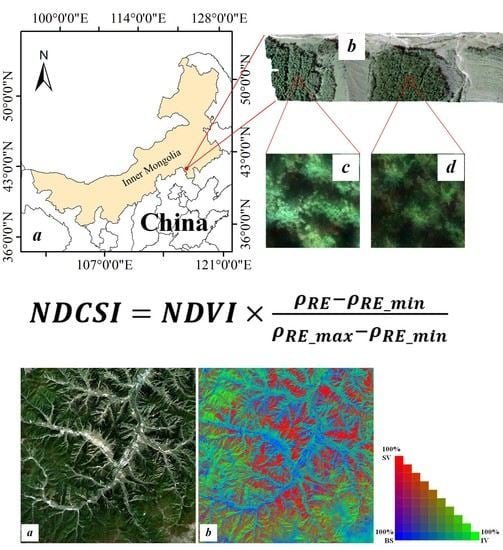
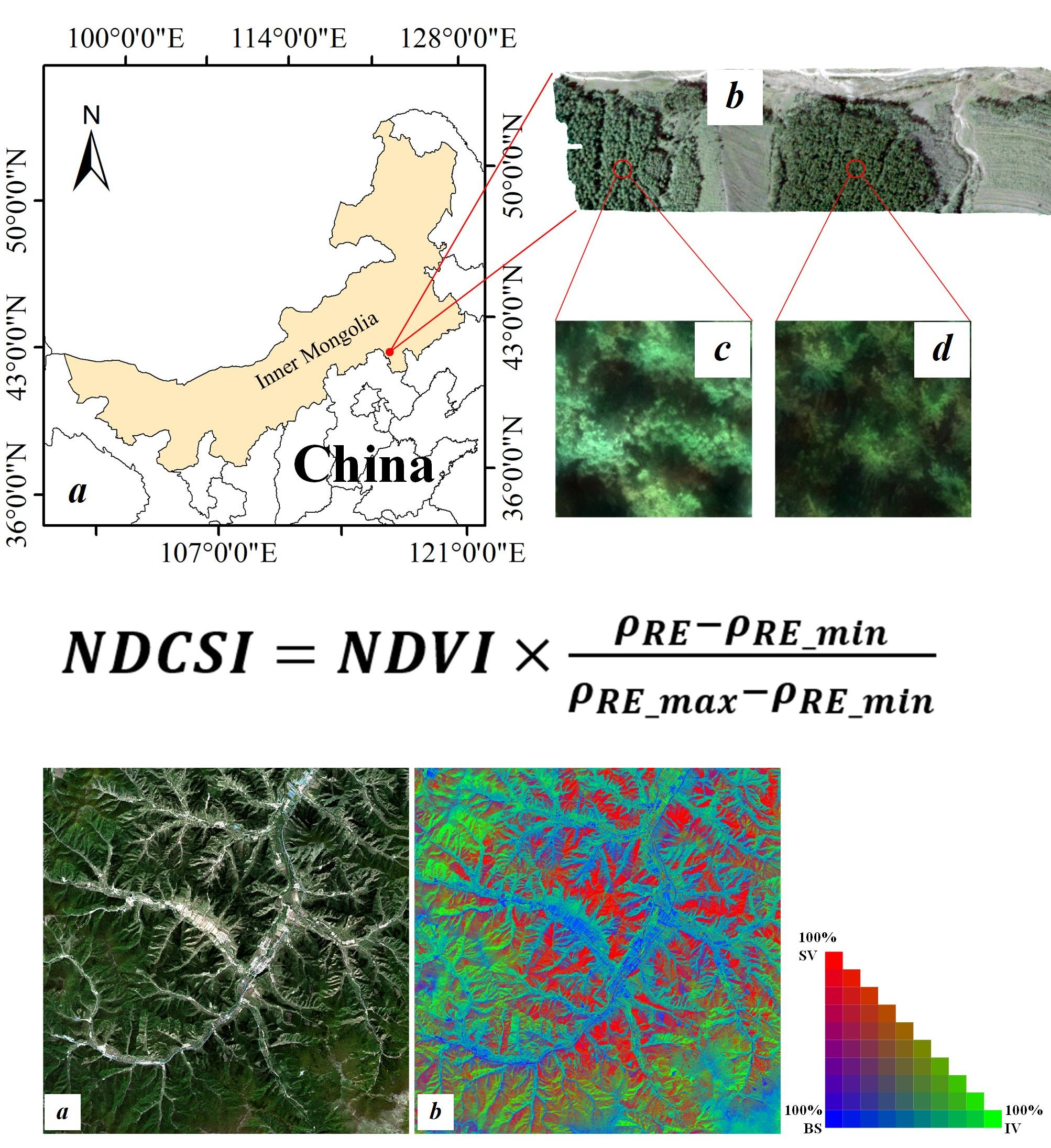
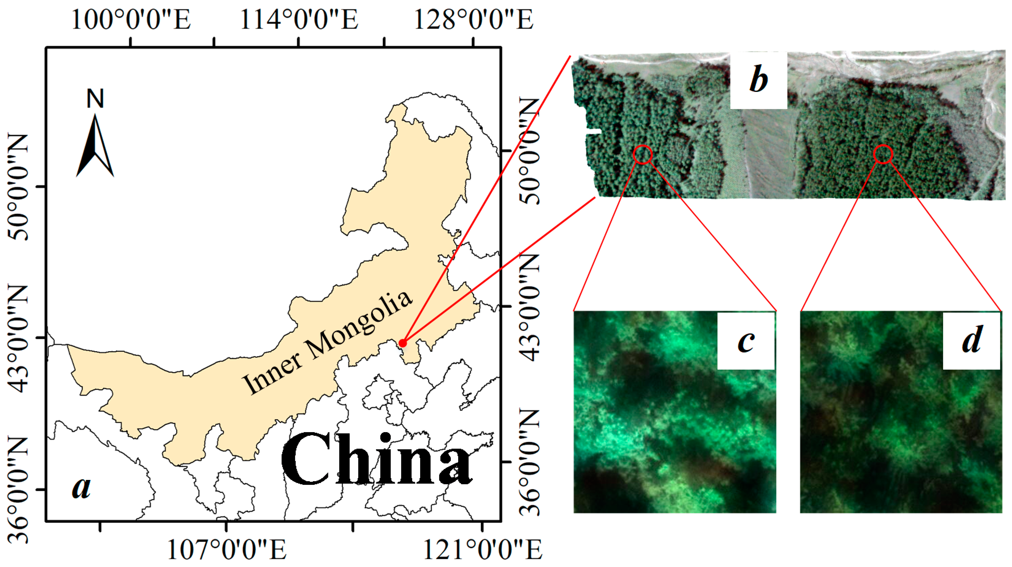
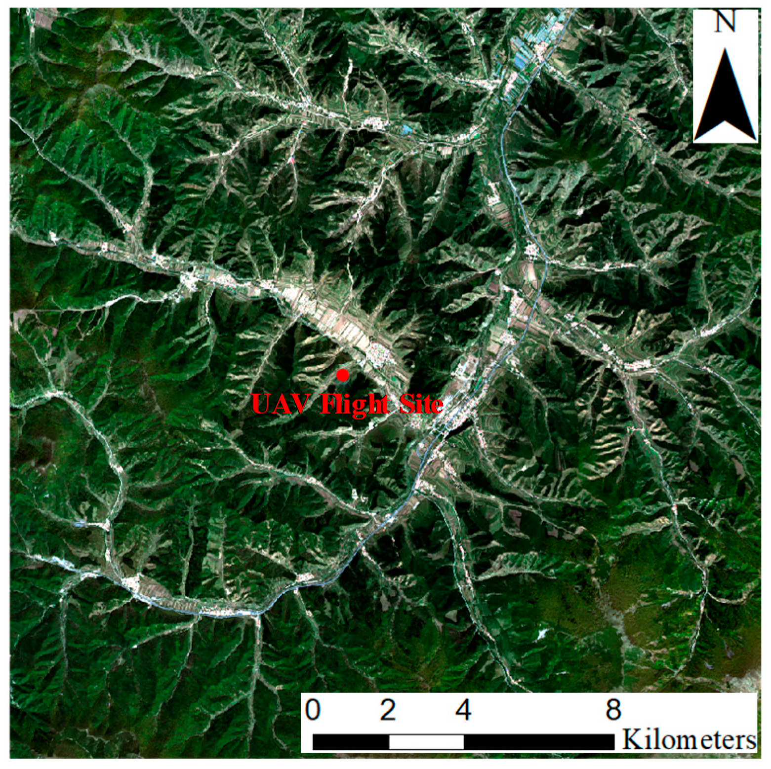
2.1. Study Area

For a study area, we chose the Wangyedian Forest Farm in Inner Mongolia, China. Its coordinates are 41°39′30.24″N, 118°19′7.25″E with an average elevation of 1000 meters approximately. The dominant tree species are Pinus tabulaeformis and Larix, both coniferous. The specific study area was on the ridge line of a mountain, with a pure, dense canopy of the two dominant trees in separate areas.

Pinus is a coniferous evergreen tree with a height of 30 meters and a diameter of nearly 1 m. The main branches are spreading or oblique, with 2-needle in a bundle of 10–15 cm long and 1.5 mm wide. Larix belongs to the Pinaceae family, with a height of up to 35 meters and a diameter of up to 90 cm. Their leaves are oblanceolate with 1.5–3 cm long and 0.7–1 mm wide.

2.2. Data Collection

2.2.1. Unmanned Aerial Vehicle Hyperspectral Image

Unmanned aerial vehicle (UAV) remote sensing has rapidly developed, having the advantages of high flexibility and high image quality [34]. A UAV flight experiment can be carried out free from atmospheric interference at a relatively low price. Field measured data for this study came from a Cubert S185 airborne imaging spectrometer (Cubert GmbH, Germany) carried by an eight-claw UAV. This UAV machine has been carried out for a study to retrieve soybean leaf area index (LAI) by comparing four regression models [35]. The features of synchronous imaging for all the spectral channel of S185 are suitable for airborne mobile measurement, and the data are real and reliable without artifacts. Different from the traditional push-scan imaging method, it adopts the frame synchronous imaging technology without any moving parts. The hyperspectral images had a spectral range of 450 to 950 nm with a spectral sampling interval of 4 nm, a spectral resolution of 8 nm at 532 nm. It has 125 spectral channels in total including all the important vegetation-related bands from visible light to near infrared. The important channels for the study are concentrated around the wavelengths of 705 nm, which is the band-5 in Sentinel-2A satellite settled for vegetation red edge. For each band, the image has a 12 bit (4096 DN) dynamic range created by projecting different bands to different parts of a charged coupled device (CCD). The flight date was Sept. 28, 2017, at a height of 250 m, and the spatial resolution was approximately 6.5 cm.

The pre-processing of the UAV hyperspectral image mainly includes the radiometric correction and accurate multi-image splicing. The radiometric calibration system is used to calibrate the hyperspectral image, converting the pixels’ Digital Number (DN) into surface reflectivity. Afterwards, the structure from motion algorithm (SFM) was used to detect the feature points satisfying the image overlap degree (course overlap >70%, side overlap >30%). The matching pairs of feature points were established, and the related image orientation was corrected according to the ground control points to achieve the image re-arrangement. The dense multiview stereo algorithm (MVS) is used to reconstruct the 3D point cloud of the rearranged image, and the digital differential inverse method is used to realize the mosaic and orthophoto correction of the image. Topographical correction and noise processing were also adopted to obtain the standard reflectance hyperspectral image, eventually as shown in Figure 1.

2.2.2. Sentinel-2 Satellite Multispectral Image

The sentinel satellites are a central part of global monitoring for environment and security (GMES), also known as the Copernican program run by European Space Agency (ESA). Sentinel-2 A/B are the second sets of satellites launched in 2015 and 2017 separately, carrying the multispectral instrument (MSI) [36]. They form a satellite constellation in a sun-synchronous orbit at a 180° phase difference, in order to shorten the return cycle of the satellite and improve the efficiency of its dynamic observation, with an altitude of 786 km, an orbital inclination of 98.62°, an image width of 290 km, and an orbital period of 100 min.

Twelve detecting elements are arranged along the scanning direction of the MSI sensor, and the ground reflection solar spectrum within the scanning band is acquired simultaneously by means of push-sweep scanning. MSI consists of 13 spectral bands ranging from 400 to 2400 nm, which cover the electromagnetic spectrum from visible light to short-wave infrared in a narrow channel width. Bands can be divided into 10 m, 20 m and 60 m resolutions according to spatial resolution. Bands with different resolutions have different purposes. Among the optical data, Sentinel-2 is the only satellite with three bands in the red edge range [37], which is very effective for monitoring vegetation health information. See

Table 1. Attributes of Sentinel-2 A/B satellite’s 13 bands.

Spatial Resolution	Spectral Band	Central Wavelength (nm)	Bandwidth (nm)	Band Names	Application Fields
10 m	B2	490	65	Blue	Epicontinental monitoring Marine monitoring The polar monitoring
	B3	560	35	Green
	B4	665	30	Red
	B8	842	115	NIR
20 m	B5	705	15	Vegetation Red Edge	Vegetation monitoring Environmental monitoring
	B6	740	15	Vegetation Red Edge
	B7	775	20	Vegetation Red Edge
	B8a	865	20	NIR
	B11	1610	90	SWIR	Ice monitoring Vegetation monitoring Geological monitoring
	B12	2190	180	SWIR
60 m	B1	443	20	Coastal aerosol	Atmospheric correction (aerosol, water vapor, cirrus)
	B9	940	20	Water vapour
	B10	1375	30	SWIR-Cirrus

for details.

Three bands related to vegetation red edge (B5, B6, B7) can be used for monitoring the status and health of plant pigment. They also have narrow bandwidth (15nm for B5 and B6, 20nm for B7) and similar central wavelength comparing to the UAV hyperspectral data used in the study. As a result, the Sentinel-2 multispectral image can be utilized to test the adaptation and application ability of the proposed Normalized Difference Canopy Shadow Index to differentiate different shadow circumstances of a vegetation canopy quantitatively and distinguish sunlit vegetation canopy from shaded ones and soil backgrounds.

Under the Copernicus program’s data policy, Sentinel-2 A/B’s level-1B and level-1C data can be downloaded for free to users worldwide. Level-1B data have been processed by a series of procedures including dark signal correction, non-uniform pixel response correction, crosstalk correction, defect pixel recognition, deconvolution and noise reduction. Level-1C data can be obtained using level-1B data through radiation correction, geometric correction based on orthophoto correction, sub-pixel precision level spatial registration and splicing.

ESA makes SNAP software specifically for Sentinel satellites. Two plug-ins, Sen2Cor and Sen2Three, are the most important parts of the SNAP software. Sen2Cor is used for atmospheric correction and cloud removal of the image. With SNAP, a processed standard reflectivity image of Sentinel-2A has been obtained at the spatial resolution of 10m. The image was produced at Sept. 22^th, 2017 and a subset including the UAV flight area was gotten with the size of 2000 * 2000 Sentinel-2 image pixels, shown as Figure 2.

2.3. Red Edge Technique

The Red Edge (RE) refers to the wavelengths at which vegetation grows fastest from 670 to 760 nm. The RE is closely related to various physical and chemical parameters of vegetation such as chlorophyll content, leaf cell structure and hydric status. The RE is a vitality indicator for surveying vegetation growth status because it is related to plant pigment status and growth health. The reflectance on the left side of RE is mainly related to the chlorophyll content, while the reflectance on the right side of RE is mainly affected by the tissue structure in the leaf and the water content in the plant. Collins [38] proposed that the shift of RE’s location in the long wave direction reflected the increase of chlorophyll concentration in plants, which was due to the increased chlorophyll concentration and the enhanced photosynthesis of plants, requiring more photons to be consumed. As a conclusion, RE’s peak value, location, and area are the most commonly used factors for hyperspectral remote sensing to monitor the chlorophyll, physiological activities, and biomasses of agricultural and forestry crops [39,40].

Obviously, there were varying proportions of light and dark pixels from the detailed tree canopy region in the UAV hyperspectral images, which caused missing or wrong spectral information in regard to species recognition. Alternative reasons may be the direction of solar irradiation, the sensor orientation, and obstructing tree components (leaves, stems, etc.). Typical leaf pixels with different illumination proportions from the two tree species were chosen; their spectra are shown in Figure 3.

The result displayed in Figure 3 shows that the overall shape of a single tree species with different proportions of shadow and illumination is highly similar, and the brighter pixel’s spectrum has an observably higher amplitude overall. The difference is very small in the blue or green bands but becomes greater in the red or near-infrared (NIR) bands. Therefore, illumination conditions can be distinguished more easily using red-nearby vegetation index related bands.

We selected 80 typical canopy pixels of Pinus and Larix with different proportions of illumination and shadow from the UAV hyperspectral image, whose spectral sampling interval was 4nm from 450 to 950nm. The interval was narrow enough, so only the sampled wavelengths of the UAV spectral are calculated, such as 450, 454, 458…946, 950, every 4 nm of the progression. Therefore, we defined that a differential transformation formula (Equation (1)) was used to calculate the first-order differential of the spectrum, whose maximum value determined the location of the RE:

$$R{\left({\lambda }_i\right)}^{\prime }=\frac{R\left({\lambda }_{i+1}\right)-R\left({\lambda }_i\right)}{\Delta \lambda }$$

(1)

where R(λ_i) is the reflectance at the wavelength of λ_i, and Δλ is the interval distance between adjacent wavelengths.

Other characters such as curve slope and reflectance can be easily obtained when the location is determined. The RE curve slope can be calculated using its former and latter wavelength (in nanometers) and the corresponding reflectance because the spectral curve in RE range is smooth enough. All data of slope and reflectance of RE from

Table 2. Red Edge Parameters of Pinus and Larix with Different Illumination/Shadow Proportions. Twenty of the 80 pixels’ parameters are listed.

ID	Location of RE (nm)	Slope of RE	Reflectance of RE
Pinus (Illumination)
1	702	49.5	0.1469
2	706	41.875	0.1686
3	706	45.625	0.1664
4	694	37.5	0.1032
5	710	43.5	0.1765
Pinus (Shadow)
6	706	15.375	0.0499
7	702	20.5	0.0492
8	710	18.875	0.0658
9	718	24	0.0984
10	718	22.875	0.0795
Larix (Illumination)
11	710	47.125	0.1219
12	718	57.125	0.1659
13	714	43	0.1426
14	718	65.875	0.1865
15	718	58.875	0.1952
Larix (Shadow)
16	710	9.625	0.0317
17	714	20.5	0.0488
18	714	14.5	0.0461
19	718	17.875	0.0568
20	706	15.5	0.0414

Note: reflectance calculated for Slope of RE was multiplied by 10,000.

are strictly calculated with corresponding bands after determination of RE’s location using Equation (1).

The precise location of RE determined using Equation (1) is required for study only using typical pixels. While for quantitative calculation of the whole image and practical application afterwards. The RE’s location should be set at a wavelength with the statistical maximum frequency of the selected canopy pixels. In this study, all original and processed data from 160 typical canopy pixels were calculated using Equation (1) to determine the location of RE. RE’s location is calculated at first. Slope and reflectance of RE are processed using wavelength according to RE’s location. As for image unified computation and satellite application, RE’s location is settled at the wavelength of 710nm with statistical results of tested pixels.

2.4. Linear Spectral Mixture Analysis

Linear Spectral Mixture Analysis (LSMA) is a widely used theory in the research of hyperspectral data and has found many applications in data analysis [41]. It describes a sample of data in a linear model that can be composed and parameterized and determined by a limited set of basic components [42]. It begins by assuming that for a given set of finite elementary substances, data samples can be modeled as a linear mixture of these substances from which data samples can be mixed into their corresponding abundance fractions. In this circumstance, the analysis of the data samples can be performed simply on these abundance fractions rather than the sample itself. The commonly used Linear Spectral Unmixing (LSU) is a technique for implementing LSMA [43].

LSU simulates the ground as flat and the incident sunlight on the ground causes the material component to radiate a certain amount of incident energy back to the sensor. Each pixel is then modeled as a linear sum of all radiation energy curves of the components that makes up the pixel. Each component contributes to the sensor’s observation in a positive linear method. In addition, energy conservation constraints are often observed, forcing the weight of the linear mixture to be positive and the sum to be one [44]. LSU usually consists of two steps: endmember extraction and computation of abundances.

A simple constrained LSU model has the following form:

$$\begin{gathered} y={\displaystyle \sum }_{i=1}^n{a}_i{f}_i+\epsilon \\ {\displaystyle \sum }_{i=1}^n{f}_i=1, and 0\le f_i\le 1 \end{gathered}$$

(2)

where y is the measured reflectance for an image pixel, a_i is the measured reflectance for endmember i, f_i is the unknown abundance or fractional cover for endmember i, $\epsilon$ is the residual between modeled and measured reflectance of the pixel, n is the number of endmembers. In this study, number of endmembers equals three.

In this study, mixed vegetation pixel of Sentinel-2 multispectral image can be divided into three components as illuminated vegetation canopy, shaded vegetation canopy and bare soil. Based on the LSMA theory, the three constituents can be restored or represented by solving the linear inverse problem of Equation (2) and their fractions can be weighted. It assumes that the mixed pixel is a linear mixture of a finite set of image endmembers, and the data samples are then decomposed by finding its abundance fractions of these endmembers for data analysis. Endmembers of illuminated vegetation, shaded vegetation and bare soil can be extracted using the scatterplot of two vegetation indexes (the proposed NDCSI and existing BSI in this case). The three vertexes of the 2-D scatterplot represent the samples of three endmembers respectively, which can be extracted and calculated in Equation (2) for the fractions.

3. Normalized Difference Canopy Shadow Index

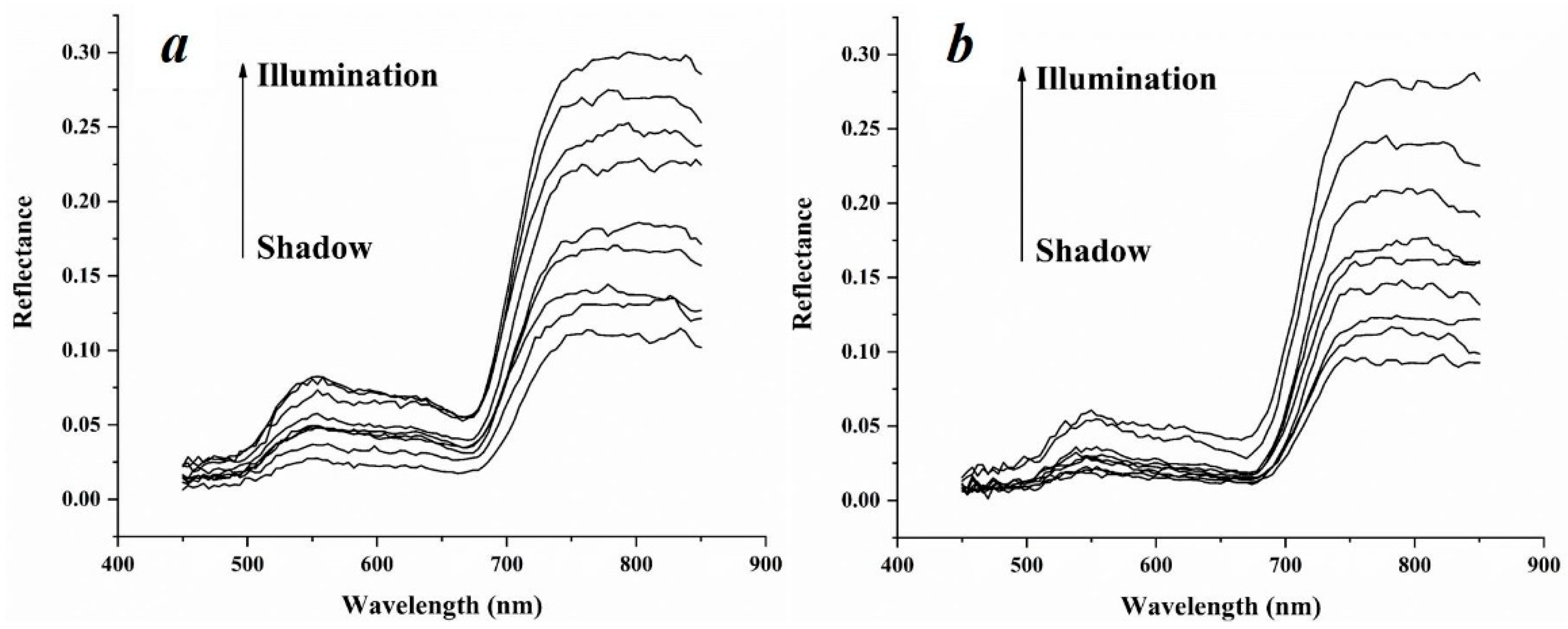
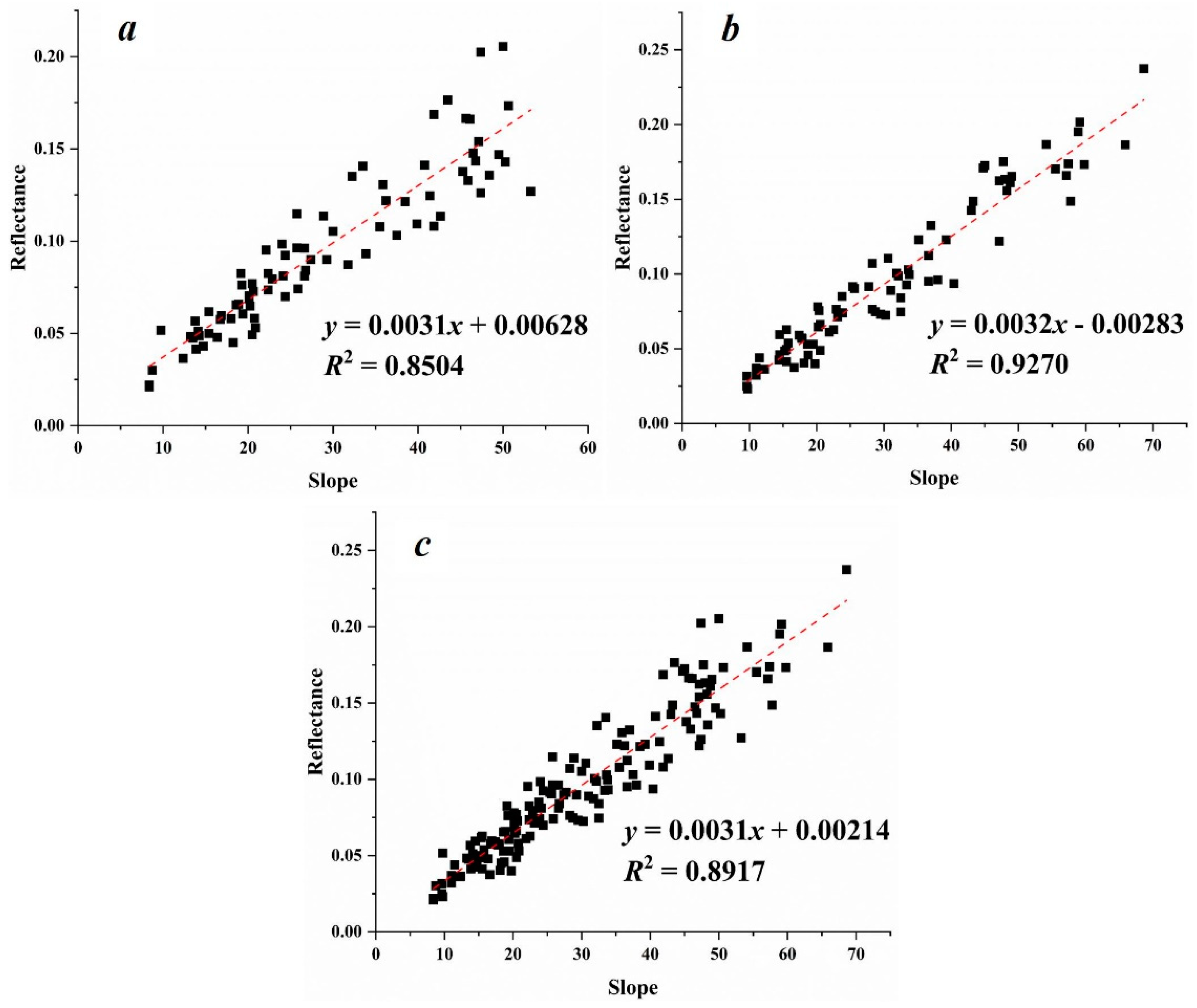
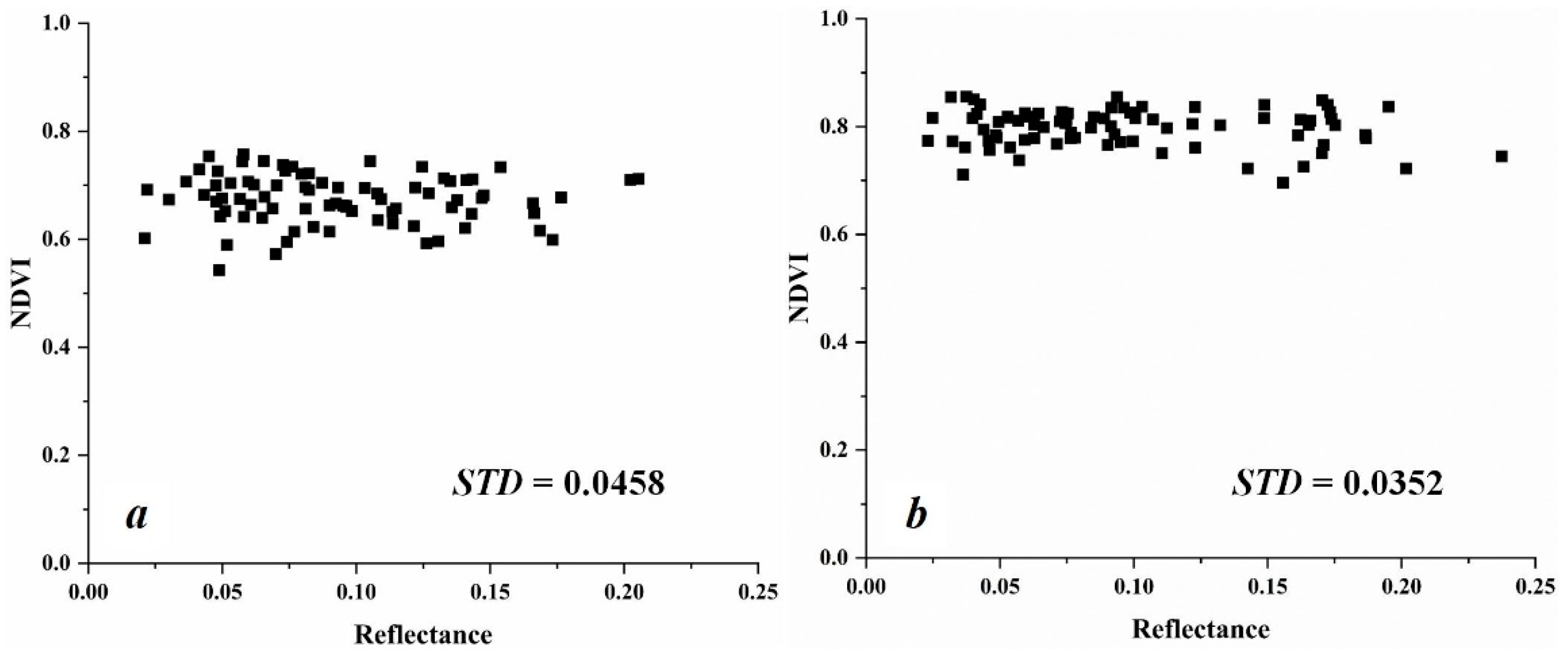
3.1. Response of Red Edge and NDVI to Vegetation Shadows

The RE’s locations for both tree species were distributed around a wavelength of 710 nm regardless of the proportion of illumination to shadow, and its slopes and reflectances changed by a large margin. Correlations between RE’s reflectances and slopes were drawn correspondingly in Figure 4 using 80 samples from a single tree species and all 160 samples together.

The R² from the three charts all reached beyond 0.850 (p < 0.01), which indicates a good linear correlation between the two parameters of the RE in either a single species or both species combined. Figure 3 shows that there is a positive correlation between the illumination proportion and the reflectance spectrum, which is especially distinctive around the red-NIR bands. Therefore, the RE’s reflectance is easily determined and can differentiate the illumination/shadow proportion of a vegetation canopy quantitatively and without regard for the tree species.

The NDVI is a classic and widely used vegetation indicator that is applied to detect vegetation growth and partially eliminate the influence of radiation error [45]. The value of the index is closely related to transpiration, photosynthesis, interception of sunlight, and the net primary productivity of the surface [46,47,48].

Correlations between the RE’s reflectance and the NDVI are shown in Figure 5 using 80 samples from each species. Standard deviation results of Pinus (0.0458) and Larix (0.0352) indicate that NDVI values are stable in a relatively narrow range without being disturbed by changes of RE’s reflectance, and can differentiate the shadow proportion of vegetation canopy quantitatively. Therefore, NDVI is suitable for constructing a new, shadow-related vegetation index. It is rarely influenced by differing proportions of canopy shadow, guarantees a stable value for vegetation morphological characteristics, and is able to distinguish green vegetation individually from a soil background.

3.2. Proposed Normalized Difference Canopy Shadow Index

We constructed the NDCSI formula [Equation (3)] based on a study of correlations between RE parameters and NDVI. The NDCSI can determine the proportion of shadows in a vegetation canopy:

$$NDCSI=NDVI\times \frac{{\rho }_{RE}-{\rho }_{RE\_min}}{{\rho }_{RE\_max}-{\rho }_{RE\_min}}$$

(3)

where ${\rho }_{RE}$ is the value of the RE’s reflectance, and ${\rho }_{RE\_max}$ and ${\rho }_{RE\_min}$ are the theoretical maximum and minimum values of RE’s reflectance in the entire image. Practically, ${\rho }_{RE\_max}$ and ${\rho }_{RE\_min}$ can be determined using thresholds within a certain range of histogram statistics (for example, from 1% to 99%).

The factor NDVI determines vegetation morphological characteristics and eliminates the effects of radiation changes partly related to atmospheric conditions. The normalized format of the NDCSI controls values ranging from 0 to 1, which benefits subsequent application.

4. Results

4.1. Results of Unmanned Aerial Vehicle Data

A sub-area of a UAV hyperspectral image of 2000 × 2000 pixels was chosen to verify the accuracy of NDCSI when determining the proportions of illumination and shadow of vegetation. Most of the area was covered with a thick Larix canopy, which prevented the influence of a soil and water background. The original image and its NDVI and NDCSI results are shown in Figure 6. Figure 6c shows an explicit result calculated using NDCSI that shows illumination/shadow portions more clearly distinguished than those in the NDVI results (Figure 6b).

Forty typical Larix canopy subarea sample images with different illumination/shadow proportions were selected and their NDCSI values calculated. In addition, an accumulated sum reflectance of the visible spectrum (400 to 760 nm) were acquired to represent the measured brightness information of the corresponding pixels. Correlations between the NDCSI and the measured brightness values are shown in Figure 7.

A single pixel’s NDCSI and measured brightness values have a close relation, with a positive correlation of R² = 0.886 (p < 0.01), which indicates that the NDCSI has an adequate capacity for quantitative expression of the vegetation canopy illumination/shadow. However, the NDCSI changes astatically and does not fit the linear equation well when the illumination value is too high (circled in red in Figure 6). The illumination saturation phenomenon is very likely caused by the factor and similar formula structure of the NDVI, which is easily saturated and less sensitive to areas of high vegetation density because of nonlinear transformation.

4.2. Results of Sentinel-2 Satellite Data

Based on Daughtry’s theory [49], it was hypothesized that in vegetation canopy, fractions of photosynthetic vegetation (PV), non-photosynthetic vegetation (NPV) and bared soil (BS) can be resolved by using the linearly independent indices NDVI and CAI. Likewise, based on Sentinel-2A multispectral data, this study contributes to resolve mixed vegetation canopy pixels into fractions of illuminated vegetation, shaded vegetation and bare soil through indices NDCSI and BSI.

NDCSI was proposed based on the UAV hyperspectral data. When applying for Sentinel-2 hyperspectral image, corresponding bands should be utilized. Band 4 and 8 of Sentinel-2A are calculated for the NDVI factor and band 5 (central wavelength at 705 nm, close to RE location of UAV data) are used as RE factor. Rikimaru [50] proposed a bare soil index (BSI) for more reliable estimation of the vegetation status where the vegetation covers less than half of the area. The basic logic of this approach is based on high reciprocity between bare soil state and vegetation state.

$$BSI=\frac{\left[\left(B5+\mathrm{B}3\right)-\left(\mathrm{B}4+\mathrm{B}1\right)\right]}{\left[\left(B5+\mathrm{B}3\right)+\left(\mathrm{B}4+\mathrm{B}1\right)\right]}$$

(4)

where B1, B3, B4, B5 refer to Landsat TM Band 1, 3, 4 and 5. Sentinel-2A has the similar band settings with Band 2, 4, 8 and 11 correspondingly.

In the scatterplot of NDCSI versus BSI, calculations of reflectance spectra from the whole Sentinel-2 image form a triangle; illuminated vegetation (IV) having a high NDCSI and intermediate values of BSI; shaded vegetation (SV) having both low NDCSI and low BSI values; bare soil (BS) having low NDCSI and high BSI (Figure 8).

Based on the conceptual approach from Figure 8, the relative abundance of each fractional cover should be resolved by LSU if the location and spectra of pure endmembers is known. Endmember spectra can be obtained directly from satellite image, measured on the ground or extracted from the spectral library. In fact, spectra derived directly from images are generally better than those derived from the ground or in the spectral library because they more accurately account for any errors in sensor calibration and atmospheric correction [43]. Using Region of Interest (ROI) tool from ENVI software and scatterplot of NDCSI versus BSI, endmember spectra of illuminated vegetation (IV), shaded vegetation (SV) and bare soil (BS) can be obtained easily and accurately.

Using LSU analysis (Equation (2)) and endmember spectra derived from the vertices of the triangle in scatterplot of NDCSI versus BSI, fractional cover results of illuminated vegetation (IV), shaded vegetation (SV) and bare soil (BS) from Sentinel-2A image (Figure 2) were obtained, shown as Figure 9.

Forty typical vegetation sample pixels with different illumination/shadow proportions were selected and their fractional illuminated vegetation cover (FIVC) values were calculated. In addition, an accumulated sum reflectance of the visible spectrum (Band 2, 3 and 4 of Sentinel-2A) were acquired to represent the measured brightness information of the corresponding pixels. Correlations between the FIVC and the measured brightness values are shown in Figure 10.

Based on Sentinel-2A multispectral data, the fitted linear relation between vegetation pixel’s FIVC and measured brightness values reached a positive correlation of R² = 0.827 (p < 0.01). The results indicated that, combined with a nonlinear dependent vegetation index (for example, BSI in this study), the NDCSI owns an adequate capacity for quantitative expression of the fractional cover of illumination/shadow vegetation canopy. The result expands the application scenarios of NDCSI and it is possible for satellite images with RE-related bands to calculate the fractional illuminated vegetation cover and extract the bright enough portion.

5. Analysis and Discussion

Vegetation illumination and shadow are relative and opposite phenomena whose proportions refer to the number of solar photons that have been reflected into the imaging spectrometer or satellite sensor. It visually appears to be brighter or darker with different degrees of illumination, and the vegetation reflectance spectra also become higher or lower, but in a similar morphological fashion. These fluctuations have greatly influenced large-scale vegetation diagnoses, such as tree species identification and forest health monitoring. Shadows resulting from the vegetation canopy exhibit significant impact on vegetation growth and can be detected using unique features of vegetation, such as red edge and photosynthetic intensity. Previous studies that focus on vegetation shadows have utilized large amounts of data and parameters, and their proposed models have considered detailed observation conditions. These models are encouraged when applied for research on a single tree or small-area forest with detailed ground measurements. Nevertheless, comprehensive surveys on large-scale areas are also important and practical, where the data sources usually depend on satellite images with several spectral bands and the earth surface is too intricate to conduct ground measurement. Quantitative expressions or measurements of illumination and shadow proportion is difficult to calculate. Models or vegetation indexes with concise forms but precise estimation abilities are necessary for satellite resources in large-scale areas.

The NDCSI was proposed using two parameters, vegetation red edge and its NDVI. These two parameters have been studied for decades and have been shown to be closely related to vegetation growth conditions and photosynthesis intensity. Vegetation red edge and NDVI display different reactions to changes in the proportions of vegetation illuminated canopy. Measured brightness values from images have been regarded as true ground samples. They were calculated and accumulated using all reflectance values from bands in the visible light range. Results from UAV data (Figure 4) indicate that red edge slope and reflectance remain positive and display a linear correlation with the change in the proportion of illuminated vegetation. In addition, the linear correlations of two tree species can be merged to obtain the same precision. Vegetation red edge is a sensitive indicator of vegetation shadow and eliminates background noise. The value of NDVI is steady, even with different vegetation illumination proportions (Figure 5), and it can describe the morphological characteristics of vegetation, even in circumstances of high shadow proportions. With these two factors, the use of NDCSI was proposed, based on the classic form of NDVI. The normalized equation is restricted to values ranging from 0 to 1, avoiding overflowed data. Results from Sentinel-2A imaging (Figure 9) have resolved the mixed multispectral data into fractional cover of illuminated vegetation and shaded vegetation using LSMA. The results indicate that NDCSI displays an advantage for further application, especially for its concise formula and easily available parameters.

The construction of NDCSI can be applied for many follow-up studies and contribute to further our understanding of shadow impacts on vegetation growth. For example, NDCSI and its theory can be used to have a long-time monitoring to observe and calculate differences of vegetation growth states between the two sides of the hillside using multitemporal satellite data. It can also be used with other vegetation indexes to unmix and exclude shadow interference and influence on satellite data. Images of not only the vegetation canopy but also the soil background can be affected by shadow phenomena. With the integration of vegetation, soil, illumination, and shadow, a more detailed and elaborate determination of fractional cover, including illuminated vegetation, illuminated soil, shaded vegetation and shaded soil, is expected to be classified using linear spectral mixture analysis in future research. The linear spectral unmixing of the four components will be refined to distinguish backgrounds and target subjects with higher accuracy and theoretical basis.

As for NDCSI’s shortage, it is a vegetation index mainly concerning about the distribution and proportion of shadows on images, but few detailed biological or chemical parameters has been taken into consideration. And vegetation canopies were regarded as flat 2-D surfaces, with no specific description of the leaves’ 3-D structure. When applied for a thorough analysis of single tree models, more parameters should be included in the NDCSI, such as leaf angle distribution, leaf area and leaf chlorophyll content. Further studies are going to be conducted in the future.

6. Conclusions

From the positive correlations and R² results between RE parameters (curve slope and reflectance) and the NDVI of vegetation canopy in different illumination/shadow proportions, we derived two fundamental conclusions: (1) the RE parameters of a vegetation canopy are able to distinguish the shadow proportion of the canopy quantitatively without being influenced by tree species, and (2) the NDVI is rarely influenced by canopy shadow proportion and guarantees a stable value for vegetation morphological characteristics. A normalized difference canopy shadow index (NDCSI) was proposed that incorporated the above analysis, and was verified to be accurate enough for a quantitative differentiation of canopy sunlight conditions.

Based on a Sentinel-2 multispectral image, NDCSI was applied for linear spectral mixture analysis (LSMA) combined with bare soil index (BSI). Positive correlations between measured brightness values and fractional illuminated vegetation cover (FIVC) proves NDCSI’s capacity of utilization for satellite images to calculate and extract the illuminated enough vegetation canopy.

References

1. Ahlstrom, A.; Xia, J.Y.; Arneth, A.; Luo, Y.Q.; Smith, B. Importance of vegetation dynamics for future terrestrial carbon cycling. Environ. Res. Lett. 2015, 10, 054019. [Google Scholar] [CrossRef]
2. Fassnacht, F.E.; Latifi, H.; Stereńczak, K.; Modzelewska, A.; Lefsky, M.; Waser, L.T.; Straub, C.; Ghosh, A. Review of studies on tree species classification from remotely sensed data. Remote Sens. Environ. 2016, 186, 64–87. [Google Scholar] [CrossRef]
3. Rautiainen, M.; Lang, M.; Mottus, M.; Kuusk, A.; Nilson, T.; Kuusk, J.; Lukk, T. Multi-angular reflectance properties of a hemiboreal forest: An analysis using CHRIS PROBA data. Remote Sens. Environ. 2008, 112, 2627–2642. [Google Scholar] [CrossRef]
4. Hasegawa, K.; Izumi, T.; Matsuyama, H.; Kajiwara, K.; Honda, Y. Seasonal change of bidirectional reflectance distribution function in mature Japanese larch forests and their phenology at the foot of Mt. Yatsugatake, central Japan. Remote Sens. Environ. 2018, 209, 524–539. [Google Scholar] [CrossRef]
5. Shao, Y.; Taff, G.N.; Walsh, S.J. Shadow detection and building-height estimation using IKONOS data. Int. J. Remote Sens. 2011, 32, 6929–6944. [Google Scholar] [CrossRef]
6. Matsuki, T.; Yokoya, N.; Iwasaki, A. Hyperspectral tree species classification of Japanese complex mixed forest with the aid of Lidar data. IEEE J.-Stars 2015, 8, 2177–2187. [Google Scholar] [CrossRef]
7. Li, Y.; Gong, P.; Sasagawa, T. Integrated shadow removal based on photogrammetry and image analysis. Int. J. Remote Sens. 2005, 26, 3911–3929. [Google Scholar] [CrossRef]
8. le Hegarat-Mascle, S.; Andre, C. Use of Markov Random Fields for automatic cloud/shadow detection on high resolution optical images. ISPRS J. Photogramm. 2009, 64, 351–366. [Google Scholar] [CrossRef]
9. Luther, J.E.; Fournier, R.A.; Houle, M.; Leboeuf, A.; Piercey, D.E. Application of shadow fraction models for estimating attributes of northern boreal forests. Can. J. For. Res.-Rev. Can. Rech. For. 2012, 42, 1750–1757. [Google Scholar] [CrossRef]
10. Yang, X.; Tang, J.W.; Mustard, J.F.; Lee, J.E.; Rossini, M.; Joiner, J.; Munger, J.W.; Kornfeld, A.; Richardson, A.D. Solar-induced chlorophyll fluorescence that correlates with canopy photosynthesis on diurnal and seasonal scales in a temperate deciduous forest. Geophys. Res. Lett. 2015, 42, 2977–2987. [Google Scholar] [CrossRef]
11. Cetin, M. Changes in the amount of chlorophyll in some plants of landscape studies. Kastamonu Univ. J. For. Fac. 2016, 16, 239–245. [Google Scholar]
12. Hernandez-Clemente, R.; North, P.; Hornero, A.; Zarco-Tejada, P.J. Assessing the effects of forest health on sun-induced chlorophyll fluorescence using the FluorFLIGHT 3-D radiative transfer model to account for forest structure. Remote Sens. Environ. 2017, 193, 165–179. [Google Scholar] [CrossRef]
13. Guerschman, J.P.; Hill, M.J.; Renzullo, L.J.; Barrett, D.J.; Marks, A.S.; Botha, E.J. Estimating fractional cover of photosynthetic vegetation, non-photosynthetic vegetation and bare soil in the Australian tropical savanna region upscaling the EO-1 Hyperion and MODIS sensors. Remote Sens. Environ. 2009, 113, 928–945. [Google Scholar] [CrossRef]
14. Zhang, Q.; Chen, J.M.; Ju, W.; Wang, H.; Qiu, F.; Yang, F.; Fan, W.; Huang, Q.; Wang, Y.; Feng, Y.; Wang, X.; Zhang, F. Improving the ability of the photochemical reflectance index to track canopy light use efficiency through differentiating sunlit and shaded leaves. Remote Sens. Environ. 2017, 194, 1–15. [Google Scholar] [CrossRef]
15. Asner, G.P.; Heidebrecht, K.B. Spectral unmixing of vegetation, soil and dry carbon cover in arid regions: Comparing multispectral and hyperspectral observations. Int. J. Remote Sens. 2002, 23, 3939–3958. [Google Scholar] [CrossRef]
16. Jia, G.J.; Burke, I.C.; Goetz, A.; Kaufmann, M.R.; Kindel, B.C. Assessing spatial patterns of forest fuel using AVIRIS data. Remote Sens. Environ. 2006, 102, 318–327. [Google Scholar] [CrossRef]
17. Zeng, Y.; Schaepman, M.E.; Wu, B.; Clevers, J.G.P.W.; Bregt, A.K. Scaling-based forest structural change detection using an inverted geometric-optical model in the Three Gorges region of China. Remote Sens. Environ. 2008, 112, 4261–4271. [Google Scholar] [CrossRef]
18. Mostafa, Y.; Abdelwahab, M.A. Corresponding regions for shadow restoration in satellite high-resolution images. Int. J. Remote Sens. 2018, 39, 7014–7028. [Google Scholar] [CrossRef]
19. Arévalo, V.; González, J.; Ambrosio, G. Shadow detection in colour high-resolution satellite images. Int. J. Remote Sens. 2008, 29, 1945–1963. [Google Scholar] [CrossRef]
20. Sinclair, T.R.; Murphy, C.E.; Knoerr, K.R. Development and evaluation of simplified models for simulating canopy photosynthesis and transpiration. J. Appl. Ecol. 1976, 13, 813–829. [Google Scholar] [CrossRef]
21. Mercado, L.M.; Bellouin, N.; Sitch, S.; Boucher, O.; Huntingford, C.; Wild, M.; Cox, P.M. Impact of changes in diffuse radiation on the global land carbon sink. Nature 2009, 458, 1014–1087. [Google Scholar] [CrossRef]
22. Sprintsin, M.; Chen, J.M.; Desai, A.; Gough, C.M. Evaluation of leaf-to-canopy upscaling methodologies against carbon flux data in North America. J. Geophys. Res.-Biogeosci 2012, 117. [Google Scholar] [CrossRef]
23. Strahler, A.H.; Jupp, D. Modeling bidirectional reflectance of forests and woodlands using boolean models and geometric optics. Remote Sens. Environ. 1990, 34, 153–166. [Google Scholar] [CrossRef]
24. Dymond, J.R.; Shepherd, J.D.; Qi, J. A simple physical model of vegetation reflectance for standardising optical satellite imagery. Remote Sens. Environ. 2001, 75, 350–359. [Google Scholar] [CrossRef]
25. Pu, R.; Landry, S. A comparative analysis of high spatial resolution IKONOS and WorldView-2 imagery for mapping urban tree species. Remote Sens. Environ. 2012, 124, 516–533. [Google Scholar] [CrossRef]
26. ZJiang, Y.; Huete, A.R.; Chen, J.; Chen, Y.H.; Li, J.; Yan, G.J.; Zhang, X.Y. Analysis of NDVI and scaled difference vegetation index retrievals of vegetation fraction. Remote Sens. Environ. 2006, 101, 366–378. [Google Scholar]
27. Zhou, G.Q.; Liu, S.H. Estimating ground fractional vegetation cover using the double-exposure method. Int. J. Remote Sens. 2015, 36, 6085–6100. [Google Scholar] [CrossRef]
28. Song, W.J.; Mu, X.H.; Yan, G.J.; Huang, S. Extracting the green fractional vegetation cover from digital images using a shadow-resistant algorithm (SHAR-LABFVC). Remote Sens.-Basel 2015, 7, 10425–10443. [Google Scholar] [CrossRef]
29. Laliberte, A.S.; Rango, A.; Herrick, J.E.; Fredrickson, E.L.; Burkett, L. An object-based image analysis approach for determining fractional cover of senescent and green vegetation with digital plot photography. J. Arid Environ. 2007, 69, 1–14. [Google Scholar] [CrossRef]
30. Li, X.W.; Strahler, A.H. Geometric-optical bidirectional reflectance modeling of the discrete crown vegetation canopy-effect of crown shape and mutual shadowing. IEEE Trans. Geosci. Remote 1992, 30, 276–292. [Google Scholar] [CrossRef]
31. Chen, J.M.; Leblanc, S.G. A four-scale bidirectional reflectance model based on canopy architecture. IEEE Trans. Geosci. Remote 1997, 35, 1316–1337. [Google Scholar] [CrossRef]
32. Leblanc, S.G.; Bicheron, P.; Chen, J.M.; Leroy, M.; Cihlar, J. Investigation of directional reflectance in boreal forests with an improved four-scale model and airborne POLDER data. IEEE Trans. Geosci. Remote 1999, 37, 1396–1414. [Google Scholar] [CrossRef]
33. Chen, J.M.; Leblanc, S.G. Multiple-scattering scheme useful for geometric optical modeling. IEEE Trans. Geosci. Remote 2001, 39, 1061–1071. [Google Scholar] [CrossRef]
34. Turner, D.; Lucieer, A.; Wallace, L. Direct georeferencing of ultrahigh-resolution UAV imagery. IEEE Trans. Geosci. Remote 2014, 52, 2738–2745. [Google Scholar] [CrossRef]
35. Yuan, H.; Yang, G.; Li, C.; Wang, Y.; Liu, J.; Yu, H.; Feng, H.; Xu, B.; Zhao, X.; Yang, X. Retrieving soybean leaf area index from unmanned aerial vehicle hyperspectral remote sensing: Analysis of RF, ANN, and SVM regression models. Remote Sens.-Basel 2017, 9, 309. [Google Scholar] [CrossRef]
36. Drusch, M.; del Bello, U.; Carlier, S.; Colin, O.; Fernandez, V.; Gascon, F.; Hoersch, B.; Isola, C.; Laberinti, P.; Martimort, P.; et al. Sentinel-2: ESA’s optical high-resolution mission for GMES operational services. Remote Sens. Environ. 2012, 120, 25–36. [Google Scholar] [CrossRef]
37. Clevers, J.; Gitelson, A.A. Remote estimation of crop and grass chlorophyll and nitrogen content using red-edge bands on Sentinel-2 and-3. Int. J. Appl. Earth Obs. 2013, 23, 344–351. [Google Scholar] [CrossRef]
38. Collins, W. Remote-sensing of crop type and maturity. Photogramm. Eng. Remote Sens. 1978, 44, 43–55. [Google Scholar]
39. Boochs, F.; Kupfer, G.; Dockter, K.; Kuhbauch, W. Shape of the red edge as vitality indicator for plants. Int. J. Remote Sens. 1990, 11, 1741–1753. [Google Scholar] [CrossRef]
40. Filella, I.; Penuelas, J. The red edge position and shape as indicators of plant chlorophyll content, biomass and hydric status. Int. J. Remote Sens. 1994, 15, 1459–1470. [Google Scholar] [CrossRef]
41. Chang, C.; Heinz, D.C. Constrained subpixel target detection for remotely sensed imagery. IEEE Trans. Geosci. Remote 2000, 38, 1144–1159. [Google Scholar] [CrossRef]
42. Liu, K.H.; Wong, E.L.; Du, E.Y.; Chen, C.; Chang, C.I. Kernel-based linear spectral mixture analysis. IEEE Geosci. Remote Sens. 2012, 9, 129–133. [Google Scholar] [CrossRef]
43. Yang, C.; Everitt, J.H.; Bradford, J.M. Airborne hyperspectral imagery and linear spectral unmixing for mapping variation in crop yield. Precis. Agric. 2007, 8, 279–296. [Google Scholar] [CrossRef]
44. Chang, C.I.; Ji, B.H. Weighted abundance-constrained linear spectral mixture analysis. IEEE Trans. Geosci. Remote 2006, 44, 378–388. [Google Scholar] [CrossRef]
45. Verrelst, J.; Schaepman, M.E.; Koetz, B.; Kneubühler, M. Angular sensitivity analysis of vegetation indices derived from CHRIS/PROBA data. Remote Sens. Environ. 2008, 112, 2341–2353. [Google Scholar] [CrossRef]
46. Huang, N.; Niu, Z.; Zhan, Y.L.; Xu, S.G.; Tappert, M.C.; Wu, C.Y.; Huang, W.J.; Gao, S.; Hou, X.H.; Cai, D.W. Relationships between soil respiration and photosynthesis-related spectral vegetation indices in two cropland ecosystems. Agric. For. Meteorol. 2012, 160, 80–89. [Google Scholar] [CrossRef]
47. Zhao, J.J.; Liu, L.Y. Linking satellite-based spring phenology to temperate deciduous broadleaf forest photosynthesis activity. Int. J. Digit. Earth 2014, 7, 881–896. [Google Scholar] [CrossRef]
48. D’Odorico, P.; Gonsamo, A.; Gough, C.M.; Bohrer, G.; Morison, J.; Wilkinson, M.; Hanson, P.J.; Gianelle, D.; Fuentes, J.D.; Buchmann, N. The match and mismatch between photosynthesis and land surface phenology of deciduous forests. Agric For. Meteorol. 2015, 214, 25–38. [Google Scholar] [CrossRef]
49. Daughtry, C.S.T.; Doraiswamy, P.C.; Hunt, E.R.; Stern, A.J.; McMurtrey, J.E.; Prueger, J.H. Remote sensing of crop residue cover and soil tillage intensity. Soil Tillage Res. 2006, 91, 101–108. [Google Scholar] [CrossRef]
50. Rikimaru, A.; Roy, P.S.; Miyatake, S. Tropical forest cover density mapping. Trop. Ecol. 2002, 43, 39–47. [Google Scholar]
Figure 1. Study site location (a) and hyperspectral data (R: 650 nm, G: 562 nm, B: 470 nm) by a UAV imaging spectrometer (b) with detailed canopies of Pinus (c) and Larix (d).
Remotesensing 11 01192 g001
Figure 2. Sub-area of processed Sentinel-2A multispectral image including UAV flight site (located at the red dot).
Remotesensing 11 01192 g002
Figure 3. Reflectance spectra of Pinus (a) and Larix (b) with different proportions of shadow and illumination. The reflectance generally decreased as the proportion of shaded canopy increased.
Remotesensing 11 01192 g003
Figure 4. Scatterplot of RE’s reflectance and slope for tree species. (a) Only Pinus. (b) Only Larix. (c) Both species.
Remotesensing 11 01192 g004
Figure 5. Scatterplot of RE’s reflectance and the NDVI for Pinus (a) and Larix (b).
Remotesensing 11 01192 g005
Figure 6. Sub-area of thick Larix canopy (a) and its NDVI (b) and NDCSI (c) results for verification.
Remotesensing 11 01192 g006
Figure 7. Scatterplot of NDCSI and measured brightness values for sub-area samples. Five values (circled in red) had a poor linear correlation because of illumination saturation.
Remotesensing 11 01192 g007
Figure 8. The conceptual approach for quantifying illuminated/shaded vegetation fractional cover using Sentinel-2A multispectral data, whose reflectance spectra form a triangle in the scatterplot of NDCSI versus BSI. Pure endmembers reflectance spectra of IV, SV and BS will be located in the vertices of the triangle. Reflectance spectra of mixed pixels of the three components will be located within the triangle.
Remotesensing 11 01192 g008
Figure 9. Result (b) of the illuminated/shaded vegetation fractional cover unmixing based on the NDCSI and BSI for the Sentinel-2A image, comparing to the processed standard reflectivity image of Sentinel-2A (a).
Remotesensing 11 01192 g009
Figure 10. Scatterplot of FIVC and measured brightness values for typical vegetation samples with different illumination/shadow proportions.
Remotesensing 11 01192 g010