Article

Spatial Distribution of Forest Fire Emissions: A Case Study in Three Mexican Ecoregions

by
María Isabel Cruz-López
1,*,
Lilia de Lourdes Manzo-Delgado
2,
Raúl Aguirre-Gómez
2,
Emilio Chuvieco
3 and
Julián Alberto Equihua-Benítez
1
1
National Commission for the Knowledge and Use of Biodiversity, Liga Periférico-Insurgentes Sur 4903, Col. Parques del Pedregal, Alcaldía de Tlalpan C.P. 14010, Cd. Mexico
2
Institute of Geography, UNAM, Investigación Científica, Ciudad Universitaria, Alcaldía de Coyocán, Cd. México C.P. 04510, Mexico
3
University of Alcala de Henares, Colegios 2, Alcalá de Henares, C.P. 28801 Madrid, Spain
*
Author to whom correspondence should be addressed.
Remote Sens. 2019, 11(10), 1185; https://doi.org/10.3390/rs11101185
Submission received: 2 April 2019 / Revised: 8 May 2019 / Accepted: 15 May 2019 / Published: 18 May 2019

Abstract

:
This study shows a simplified approach for calculating emissions associated with forest fires in Mexico, based on different satellite observation products: the biomass, burnt area, emission factors, and burning efficiency. Biomass loads were based on a Mexican biomass map, updated with the net primary productivity products. The burning efficiency was estimated from a Random Forest Regression (RFR) model, which considered the fuel, weather and topographical conditions. The burned areas were the downloaded Maryland University MCD64c6 product. The emission factors were obtained from well-known estimations, corrected by a dedicated US Forest Service and Mexican campaign. The uncertainty was estimated from an integrative method. Our method was applied to a four-year period, 2011–2014, in three Mexican ecoregions. The total burned in the study region was 12,898 km2 (about 4% of the area), producing 67.5 (±20) Tg of CO2. Discrepancies of the land cover maps were found to be the main cause of a low correlation between our estimations and the Global Emission Database (GFED). The emissions were clearly associated to precipitation patterns. They mainly affected dry and tropical forests (almost 50% of all emissions). Six priority areas were identified, where prevention or mitigation measures must be implemented.

1. Introduction

The greenhouse gas (GHG) effect is a natural process that helps to maintain the thermal balance for life on Earth. However, the atmospheric composition is changing as a result of human activities, such as the burning of fossil fuels (coal, oil, natural gas), deforestation, and forest degradation. The consequent increase in GHGs has been associated with a rise in global temperatures [1,2,3], including in the period 2011–2015, which has been the warmest on record [4]. Wildfires contribute between 24% and 35% of carbon dioxide (CO2), carbon monoxide (CO), Nitrogen Oxide (NOx) and methane (CH4) emissions to the atmosphere, as well as a significant quantity of aerosols [5]. For this reason, and because of its role in vegetation changes, fire disturbance has been designated an Essential Climate Variable (ECV) [5] by the Global Climate Observing System (GCOS) to better understand Climate Change trends [6]. The GHGs associated with forest fires are CO2, CH4, and nitrogen oxides (NOx). CO is not a GHG, but it generates ozone (O3) in the troposphere and has a deleterious effect on living organisms [7]. These gases are the result of chemical reactions resulting from the combination of three components: vegetation, heat, and oxygen [8]. Their emissions vary spatially and temporally, depending on the fuel moisture conditions: the more moisture, the lower the gas emissions (owing to incomplete combustion) [9,10].
Earth observation data are essential for monitoring natural and anthropogenic processes. Their application can contribute to estimations of emissions, owing to the timely and reliable flow of information; the results can be spatially comparable, and this is an ideal method for estimating emissions from fires. Of the various methods previously proposed, the bottom-up approach [11] has been the most commonly used. It considers four main variables: biomass loss, burned area, burning efficiency, and emission factors. These variables can be ascertained from statistical, cartographic, or satellite data. A variation of this model uses the Fire Radiative Power (FRP), estimated from the radiance detected by satellite middle infrared sensors, as a surrogate of the biomass consumed by the fire [12]. However, this method has some limitations, as polar orbiting satellites have only a few observations on a single-fire activity, while geostationary satellites may miss small fires because of their coarse spatial resolution.
Remote sensing products have been used to calculate GHGs for various initiatives. The most relevant is the Global Fire Emissions Database (GFED) [13]. The GFED generates and publishes information, at the global and regional levels, about gases derived from biomass burning, following the proposal by Seiler and Crutzen [11]. A similar system is the Global Fire Assimilation System (GFAS), which uses the FRP method [14], within the framework of the Copernicus Atmosphere Monitoring System (CAMS). Other authors have worked at a regional level, such as North America [15] and southern Africa [16], or at a national level, such as Colombia [17], using Moderate Resolution Imaging Spectrometer (MODIS) products.
The GHG emissions associated with forest fires in Mexico are an annual phenomenon and are of great importance in view of their impact on the natural, social, and economic sectors at the local and regional levels, e.g., the damage to biodiversity and closure of schools. The direct effects on local areas can expand into other areas and territories by the drift of emissions. The interannual variation in emissions is associated with meteorological conditions that favor fire ignition, propagation, and extinction. The main factors in Mexico are the seasonal distribution of precipitation and the phenology of vegetation. Human activities have also been decisive in the generation of forest fires and, therefore, in the emissions, as most Mexican forest fires are anthropogenic [18]. The emissions from forest fires have been calculated in Mexico mainly from statistics supplied by CONAFOR (the National Forestry Commission) and cartography from INEGI (the National Institute of Statistic and Geography) [19,20,21,22]; these calculations followed the guidelines of the Intergovernmental Panel on Climate Change (IPCC). Nevertheless, the accuracy of the estimation can be enhanced by using satellite products to extract temporal and spatial variations.
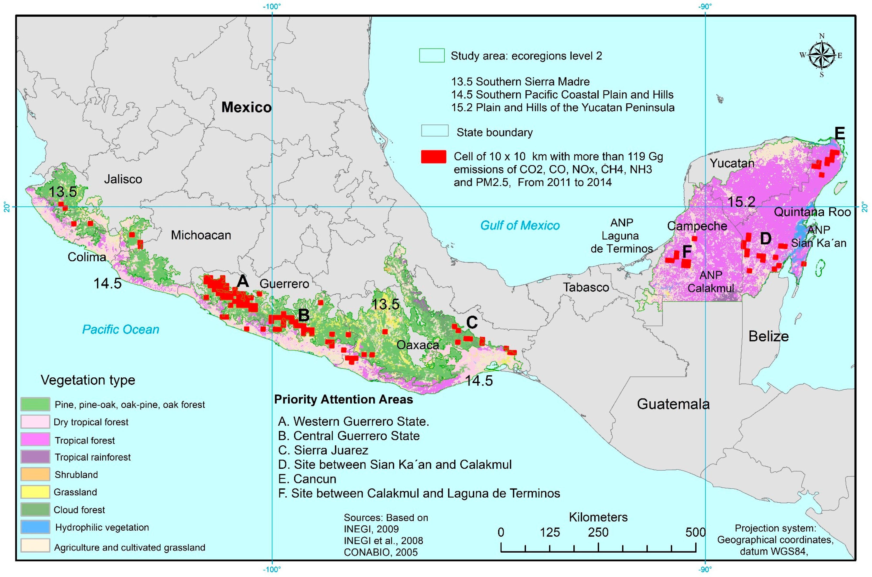
The objective of this paper is to calculate the emission of gases (CO2, CO, CH4, NOx, NH3) and fine particulates (PM2.5) caused by forest fires in three ecoregions of Mexico using remote sensing products and auxiliary data. Such knowledge regarding the spatial and temporal distribution of emissions can identify the most sensitive areas. The purpose of this paper is also to demonstrate the use of indirect techniques supported by remote sensing products with a high temporal resolution, together with a machine learning approach, in order to estimate the burning efficiency.

2. Materials and Methods

2.1. Study Area

Three ecoregions in southwestern and southeastern Mexico, 22°0′–15°3′N and 86°30′–105°45′W, were selected for the study (Figure 1). The three ecoregions are forest dominated and susceptible to fires, but they differ in their natural characteristics and ecological response. These are 3 of the 22 ecoregions recognized by the ecoregion map of Mexico [23], and were selected according to the following criteria: (1) representative area of a forest ecoregion; (2) located within political states reporting a high incidence of forest fires (CONAFOR); (3) ecoregion with active fires identified with the Early Warning Forest Fires System, operated by the National Commission for Knowledge and Use of Biodiversity (CONABIO) [24]. The three ecoregions selected were: (a) Southern Sierra Madre (ecoregion 13.5), dominated by temperate forests (e.g., pine, oak, pine-oak, and cloud forests); (b) Southern Pacific Coastal Plain and Hills (ecoregion 14.5), characterized by dry and tropical forests; and (c) Plain and Hills of the Yucatan Peninsula (ecoregion 15.2), dominated by tropical forests.

2.2. Variables for Estimating Emissions

The selection of satellite and cartographic products for calculating the emissions was based on the factors proposed by Seiler and Crutzen (1980) and on Equation (1) [25]:
M i , j , k =   B L i , j , m B E i , j , m B S i , j E k 10 15  
where M i , j , k is the amount of gas k released for a specific area (with the coordinates i, j) in Tg, B L i , j , m is the biomass load for the same area (g m−2) (assuming the area has a homogeneous cover of fuel of vegetation type m), B E i , j , m is the burning efficiency (0–1, dimensionless) of the fuel/vegetation type m, B S i , j is the burned surface of the same area (m2), and E k (Emission Factor) is the amount of trace gas k released per unit of dry matter (g kg−1 of biomass). The data used for each parameter are described below.

2.2.1. Biomass

The goal was to establish a base map of the biomass and to update it for each year of interest. The distribution of the aboveground carbon stocks of woody vegetation in Mexico was selected as the base map [26,27], because it (1) uses field and remote sensing data with similar dates, (2) has been validated, and (3) covers the whole of Mexico with a 30 m spatial resolution. The biomass was estimated by applying conversion factors for the vegetation type, as proposed in [28], and it was resampled to 500 m.
Annual updating was performed using Net Primary Production (NPP), which is defined as the generation of organic material that plants accumulate in their tissue, as a result of photosynthesis by unit area [29,30]. NPP was extracted from MOD17A3 data [31] for the Gross/Net Primary Production (GPP)/(NPP). To estimate the biomass based on NPP, a conversion factor of 0.48 [28] was used. We applied the same conversion factor for the whole study area, because NPP is an annual product and has a coarse spatial resolution (1 km2), while the biomass map was made for a specific period and has a higher spatial resolution. Both products, the base map and the annual biomass from NPP, were combined for an estimate of the biomass for a specific year.

2.2.2. Burning Efficiency

The burning efficiency corresponds to the fraction of the biomass or fuel consumed by the fire in a specific area; Mexican studies have used default values from general tables, or [19] have used information from the CONSUME model, which was designed specifically for the USA [19]. Here, we propose a Random Forest Regression (RFR) model, which has been extensively used in the last years for satellite classification, including forest fire studies [32]. This used the field data of fuel loads and their consumption, from 67 prescribed burnings in 2006 and 2007 (in 200 m2 areas) in the following types of vegetation: oak, oak-pine, pine, pine-oak, cloud forest, shrubland, dry tropical forest, tropical forest, and tropical rainforest (data supplied by Dr. German Flores Garnica, National Institute of Forestry, Agriculture and Livestock Research [INIFAP]).
The burning efficiency was calculated with a Random Forest in the regression mode. The model was implemented in the R programming language. The variables used to create the model included fuel, weather conditions, and topography, all of which affect fire behavior. The following variables were considered: (a) the above-mentioned biomass carbon map, (b) a land use and vegetation map (1:250,000) produced by INEGI, (c) land cover maps for 2005 and 2010 produced with MODIS data at a 250 m spatial resolution [33], (d) Vegetation Continuous Field products (MOD44), downloaded from the MODIS web page, and (e) a time series of the Normalized Difference Vegetation Index (NDVI) and Enhanced Vegetation Index (EVI) at a 250 m spatial resolution in a composite of 16 days. We used the difference between the vegetation indices before and after each fire. In this case, both vegetation indices were used in order to select the best option. The weather conditions were obtained through a 100 h fuel moisture model, which used MODIS and Tropical Rainfall Measuring Mission (TRMM) data [34] for the temperature and precipitation and which applied the Tetens–Murray equation [35]. The model uses the flow of moisture into the types of fuels from one day to another [34]. The topography was expressed through a digital elevation model in terms of three indicators: altitude, slope, and aspect.
The final RFR model consisted of 1000 trees. The individual tree predictions were then aggregated using the mean statistic. The coordinates of 67 areas of prescribed burning were characterized with 37 variables obtained from the above-mentioned cartographic and satellite products, in accordance with the date of the burning. The RFR model was assessed by means of the out-of-bag (OOB) estimations of accuracy (e.g., the correlation between the observed and predicted values), and the importance of the explanatory variables for the RFR model. In each run of the algorithm, the indicators were changed or removed depending on the importance of their participation in the RFR model. The method is described with more detail in [36]. The resulting RFR model was tested on the burned areas identified in March 2006.

2.2.3. Burned Areas

The burned areas were defined as the areas affected by forest or agriculture fires and are characterized by the presence of coal and ash, by the removal of vegetation, and by the alteration of the structure of the vegetation [6,37,38]. MCD45 and MCD64 satellite products, which are generated from the MODIS data, were evaluated and compared with the burned areas that were identified in high resolution images and polygons from fieldwork (CONAFOR). MCD64 was selected because it identifies burned areas better than MCD45 does; it displays burned and unburned pixels with a 500 m spatial resolution by showing persistent changes in the surface identified with the normalized difference between the MODIS bands 5 and 7, as well as by applying a dynamic threshold using the spatial and temporal distribution of active fires [39]. In October 2016, MCD64 Collection 6 was published with improvements. We validated this product with Landsat images from 2014 and 2017 by following the method described in [40].

2.2.4. Emission Factor

The emission factor is the amount of a compound released in grams per kilogram of fuel consumed (g/kg). The data in [41] have been widely used, but they are at the global level; thus, in this work, we used emission factors that were measured during a campaign in Mexico as part of the Megacity Initiative Local and Global Research Observation (MILAGRO) project, which was developed by the US Forest Service and Mexican agencies, including CONAFOR [42]. For this study, those results [42] were complemented with the work of [43], since the MILAGRO project did not consider two types of vegetation involved in the prescribed burnings.

2.3. Estimation of Emissions

Once the data were selected for estimating the parameters in Equation (1), we calculated the emissions for four years: 2011, 2012, 2013 and 2014. These years were selected because CONAFOR recorded that the year 2011 had the second highest number of forest fires and burned areas, with 1998 having had the highest since 1970, because of the El Niño phenomenon that started in 1997. In 2013, the number of fires had increased again. Consequently, the years 2011 and 2013 represent high numbers of forest fires, and the years 2012 and 2014 represent lower numbers.
The pixels identified as burned sites in MCD64A1 Collection 6 were characterized by the vegetation type, and the day of year (DOY) was transformed into the proper date. Pixels identified as natural vegetation were selected, eliminating those in cultivated areas. These selected pixels were characterized through a data cube generated with eight indicators of fuel and weather, according to the date of burning. The burning efficiency, which was calculated from the RFR model, was overlaid on the maps of the biomass and vegetation types; the latter is associated with the emission factors. The calculated emissions (Equation (1)) were integrated into cells of 10 × 10 km for their cartographic representation.

2.4. Uncertainty Calculation

The calculation of the four parameters to estimate the emissions with the remote sensing data entailed several assumptions that are considered to be valid; these assumptions were made because of a lack of field data, incomplete knowledge, and inherent data characteristics. Moreover, the spatial and temporal resolution and the minimum map unit generalize the information, so systematic and random errors are generated. Therefore, the uncertainty associated with the data can be estimated as [44]:
U t o t a l =   U 1 2 + U 2 2 + U 3 2 + U n 2 ,
where: U i 2 (i = 1, n) is the percentage uncertainty associated with each of the parameters, and U t o t a l is the percentage uncertainty of the product of the parameters.
The data used were (a) accuracy data of the biomass map [26]; (b) an accuracy matrix to validate the MCD64A1 product (burned area) using Landsat data, with a resulting accuracy of 0.79 and the calculation of the confidence interval of the producer accuracy [45]; (c) the prediction interval used to obtain the confidence interval, within an error of a critical value (t) and 95% confidence level; and (d) a confidence interval for the emission factors, calculated for each gas with an error formula with a critical value (t) and 95% confidence level.

2.5. Comparative Analysis

The results developed using the methods described above were compared with the GFED data. The GFED information has a spatial resolution of 0.25°, and the percentage of burned area was estimated [46,47] to calculate emissions using the method proposed in [48]. The GFED annual files from 2011 to 2014, together with the GFED carbon emission algorithm, were downloaded. The algorithm is useful for calculating emissions by region and vegetation cover. The algorithm code was modified to generate a raster file of emissions within a cell of 0.25°, since the original code only provides the results as a table. The carbon emissions were calculated from the measured data (annual biomass, burned area [MCD64 C.6], burning efficiency calculated with the RFR model), but the emission factors were based on the GFED information. The pixel results were incorporated into a cell of 0.25° for a spatial comparison of the results.

3. Results

3.1. Variables to Estimate Emissions

3.1.1. Biomass

The map (Figure 2) shows high biomass values in the mountain in the ecoregion Southern Sierra Madre (13.5), which is characterized by temperate forests, as well as in the ecoregion Plain and Hills of the Yucatan Peninsula (15.2), where tropical forests dominate. The values were intermediate in the Southern Pacific Coastal Plain and Hills (14.5). Figure 3 shows the four annual biomass results, and Table 1 lists the correlation between the biomass map and biomass from NPP. Both biomass products have a similar behavior in each year, with differences in the quantity of the biomass as a response to meteorological conditions. The NPP data allowed for the interpretation of annual changes and the annual adjustment of the biomass variable.

3.1.2. Burning Efficiency

For the Random Forest Regression (RFR) model, the OOB estimate yielded a correlation of 0.73 between the observed and predicted values, an absolute error of 0.079, and an RMSE (Root Mean Square Error) of 0.009. The model explained 49% of the variance in the data. The variables with a higher importance in the RFR model were (Figure 4): the vegetation type, land cover, biomass, VCF (Vegetation Continuous Field) tree cover, and 100 h fuel moisture; of these variables, the fuel moisture was the most dynamic variable (daily) and had a coarser spatial resolution. The least important variables were the VCF short vegetation cover, VCF bare ground cover and EVI; this last variable is dynamic, because it changes throughout the year.
The variables had three different spatial–temporal characteristics: (a) Permanent or referential, such as the field data on the vegetation type, complemented with the map of the land use and vegetation, and the biomass data from a map [26]. (b) The annual variation, such as the land cover (2005), tree cover percentage, no tree cover percentage, and without vegetation cover percentage coming from VCF. (c) The intra-annual variation, which is associated with the relative differences in EVI of 16-day composites; the difference was calculated from one composite before and one after the fire (defined by the burned area date), and the 100 h fuel moisture for a specific date. These characteristics may be an influence on the burning efficiency behavior.
We used prediction intervals calculated by Quantile Regression Forest [49], as an evaluation element. The prediction intervals were the widest for tropical forests (maximum ±0.2), and the narrowest for temperate forests (minimum ±0.04). Temperate forests had the highest values of burning efficiency and a higher correlation than tropical forests. Table 2 lists the burning efficiency estimated by RFR model applied to burned areas of March, 2006, in contrast to the data presented by CONAFOR [50]. These estimates range from 0.37 in dry tropical forests to 0.61 in oak forests. The higher values correspond to oak vegetation, followed by tropical vegetation. The lowest estimates correspond to pine vegetation. There were not large variations between the estimates of the same vegetation type; in all cases the differences between the maximum and minimum values were smaller than 0.19. The values estimated by the RFR model were consistently lower than those of CONAFOR. The estimates most similar to those from CONAFOR were registered in tropical forests, and those that were most different were in dry tropical forests.

3.1.3. Burned Area

The improvements in MCD64 Collection 6 identified 52% more burned areas than version 5.1 did. The validation using Landsat imagery indicated an underestimation in the identification of the burned areas from the MCD64 product, especially when the burned areas were both few and small in extent, because of the coarse spatial resolution of the MODIS data. For instance, for the wet year 2014, an omission error of 80% was observed. The accuracy can be improved in years with more forest fires and large burned areas, such as in 2017, which has a 70% accuracy, with less than 30% in omission and commission errors.
Figure 5 shows all of the burned areas identified by the MCD64 product in the period of 2011–2014. Spatially, zones with a concentration of burned areas were identified, as in the Guerrero and Oaxaca States into Southern Sierra Madre and Southern Pacific Coastal Plain and Hills ecoregions, or in the Yucatan and Campeche States into Plain and Hills of the Yucatan Peninsula ecoregion. Temporarily, there were large differences in the period; 2014 reported less than 1000 km2, in this case we expect fewer emissions. Meanwhile, other years reported more than 2000 km2 of burned areas. The extreme case was in 2013, when were reported more than 5000 km2 of burned areas, which could be translated into eight times more emissions that in 2014.

3.1.4. Emission Factors

The emission factors used in this work were selected for CO2, CO, CH4, NOx, and NH3 gases and PM2.5 particles. Table 3 lists these used emission factor. CO2 was the most abundant gas with values between 1603 g/kg in pine-oak forests and 1657 g/kg in tropical rainforests, and NH3 was the least abundant, with 0.5 g/kg in oak forests and 2.4 g/kg in tropical forests. The information was complemented with published data [43] for pine forests and desert shrubland.

3.2. Spatial and Temporal Distribution of Emissions

The accumulated emissions of CO2, CO, CH4, NOx, and NH3 gases and PM2.5 particles for the four years in our study area were 67.5 (±20) Tg, over a surface of 12,898 km2. The uncertainty of emissions (29%) was lower than that reported elsewhere [19] (47%). Figure 6 shows the annual spatial distribution of emissions in cells of 100 km2, and Table 4 lists the total emissions.
The emissions were highest in 2013 (27.5 Tg), accounting for 40.8% of the four-year total, with a burned area of 5272.75 km2. The spatial distribution was more uniform in 2013 than in the other years (Figure 6C): 53.8% in the Southern Sierra Madre ecoregion (13.5); 28.1% in Plain and Hills of the Yucatan Peninsula (15.2); and 18.1% in Southern Pacific Coastal Plain and Hills (14.5). In contrast, in 2014, the emissions were 2.9 Tg, representing 4.2% of the four-year total, with a burned area of 657.25 km2. Furthermore, the concentrations of gases were low (Figure 6D); 2014 was a wet year, with precipitations in May exceeding the May four-year average, with 45 mm in Oaxaca State and >93 mm in Yucatan. The emissions in the other two years were moderate: 21.9 Tg (32.4%) in 2011 with 4214.25 km2 burned; 15.2 Tg (22.6%) in 2012 with 2753.75 km2 burned. The emissions were concentrated in specific areas as a consequence of the drought distribution in Mexico. In 2011, 48.7% of the emissions were from Plain and Hills of the Yucatan Peninsula (ecoregion 15.2), 4.8% more than those from Southern Sierra Madre (ecoregion 13.5), where the highest percentage is usually recorded (Figure 6A). This increase was due to the low precipitation in April and May in 2011 compared with the same months in the other three years: 10 mm lower in Campeche State, 36 mm lower in Tabasco in April, and 111 mm lower in Quintana Roo in May. In this part of Mexico, 2011 was a year of extreme drought [51]. In 2012, 71.9% of emissions were in Southern Sierra Madre (ecoregion 13.5), in contrast to the 8.0% in Plain and Hills of the Yucatan Peninsula (15.2) (Figure 6B). May 2012 was the second driest May in the four years that were analyzed, with precipitations varying from 12 mm lower than the overall mean in Oaxaca to 18 mm lower in Michoacan. The year 2012 was abnormally dry in Guerrero and Oaxaca [52].

3.3. Emissions and Precipitation

Emissions were associated with the distribution of precipitation in Mexico [53] (Figure 7). Two seasons were identified: wet from May to October; and dry from November to April. The concentration of emissions in the dry season has two main causes: (a) the vegetation’s susceptibility to burning in the driest months, and (b) the use of fire in agricultural activities. In Mexico, the months with the highest activity of agricultural burning are those in the early part of the year (e.g., in 2017 the prescribed burning in Campeche State was from 12 March to 31 May).
The month with the highest emissions was one month after the driest month and before the wet season; therefore, May, April, and March had >90% of all emissions. The remaining 10% was distributed mainly among the other months of the dry season, with a smaller proportion in the wet season months. In none of the four years were there emissions recorded in September, the month before the end of the wet season and often the month with the highest precipitation. Only two years showed any emissions in August (0.03%) or October (0.01%). The 2013 wet season was the wettest of the four years; hence, in 2014, fires were fewer and the emissions were the lowest (Figure 7). The dry season in 2013 was the driest, and it had the highest emissions.

3.4. Emissions and Vegetation Type

Table 5 lists the annual percentage of emissions by vegetation type. Tropical forests accounted for the highest percentage of emissions: >29.4% in 2011, 2014, and 2013. This type of vegetation is distributed in Plain and Hills of the Yucatan Peninsula (15.2) and Southern Pacific Coastal Plain and Hills (14.5) (Figure 1). Dry tropical forests have lower emissions but a greater variability, from 8.2% to 17.4%. In 2012, emissions were distributed more uniformly in temperate forests, such as pine-oak, oak-pine, and oak in the 13.5 Southern Sierra Madre ecoregion, with the percentage in tropical forests at <15%. In cloud forests, which are restricted to the mountainous area in that ecoregion, the burned pixels ranged between 2.7% and 4.9% over the four years. Meanwhile, the emissions generated in tropical rainforests and hydrophilic vegetation represented less than 1% for all of the years; the former was restricted to small areas of the ecoregions 15.2 and 13.2, and the latter was limited to the coastal zone of the ecoregions 15.2 and 14.5. Grassland produced emissions at low percentages, between 3.7% and 5.9%, in all periods with the exception of 2014, when they reached 12.0%.
The annual emission dynamic depends on the distribution of vegetation and precipitation. In January, the vegetation type that had more emissions was grassland, because it is light fuel and quickly loses the moisture that it accumulates during the wet season. As each year progressed, emissions significantly increased in temperate forests, reaching more than 50% in May and June, while in tropical forests the emissions decreased. In July, emissions were generated in the tropical forests. By the end of the year, emissions had again increased in temperate forests and grassland. Therefore, under the conditions described here, the distribution of emissions at the ecoregion level is due mainly to environmental characteristics.

3.5. Areas of Interest in Terms of Emissions

Six areas were considered to be of interest because of a concentration of cells with emissions exceeding 119 Gg and because they were spatially continuous (Table 6 and Figure 8). Three areas were in temperate forests and the remainder were in tropical forests. The origin of forest fires in these areas is associated with agricultural activities and urban expansion; e.g., in Cancun, the cells with a concentration of emissions were along the highway and close to the urban area. When fire used in agricultural and urban activities loses control and involves natural vegetation, it is considered a forest fire.

3.6. Comparative Analysis of Results with Global Fire Emissions Database (GFED)

The present estimates of carbon emissions during 2011 and 2013 were similar to the GFED data for forested areas (Table 7). However, in all years except 2011, there was a lack of correlation because of strong local discrepancies. The highest coincidence in the estimated amount of carbon was in 2013 in Plain and Hills of the Yucatan Peninsula (ecoregion 15.2), and the lowest was in 2012 in Southern Sierra Madre (13.5). In the latter, the cells with the highest emissions identified by GFED were towards the south of the cells with the highest emissions identified by this work. The MCD12Q1 land cover product, which is an input of GFED, identifies this zone as woody savannas, whereas the INEGI cartography of Mexico identifies it as oak forests, located on the leeward side of Southern Sierra Madre, where the climate is drier than that of the windward side. In the GFED, the savanna is not considered to be a forest. Hence, differences in the cartography of the Southern Sierra Madre are the main source of discrepancy in the results. In contrast, the correlation was higher when there were more emissions in the Plain and Hills of the Yucatan Peninsula (15.2) ecoregion. Another element to consider is the difference between the versions of the burned area product; the present work used the latest version (Collection 6), whereas GFED uses a previous version.

4. Discussion

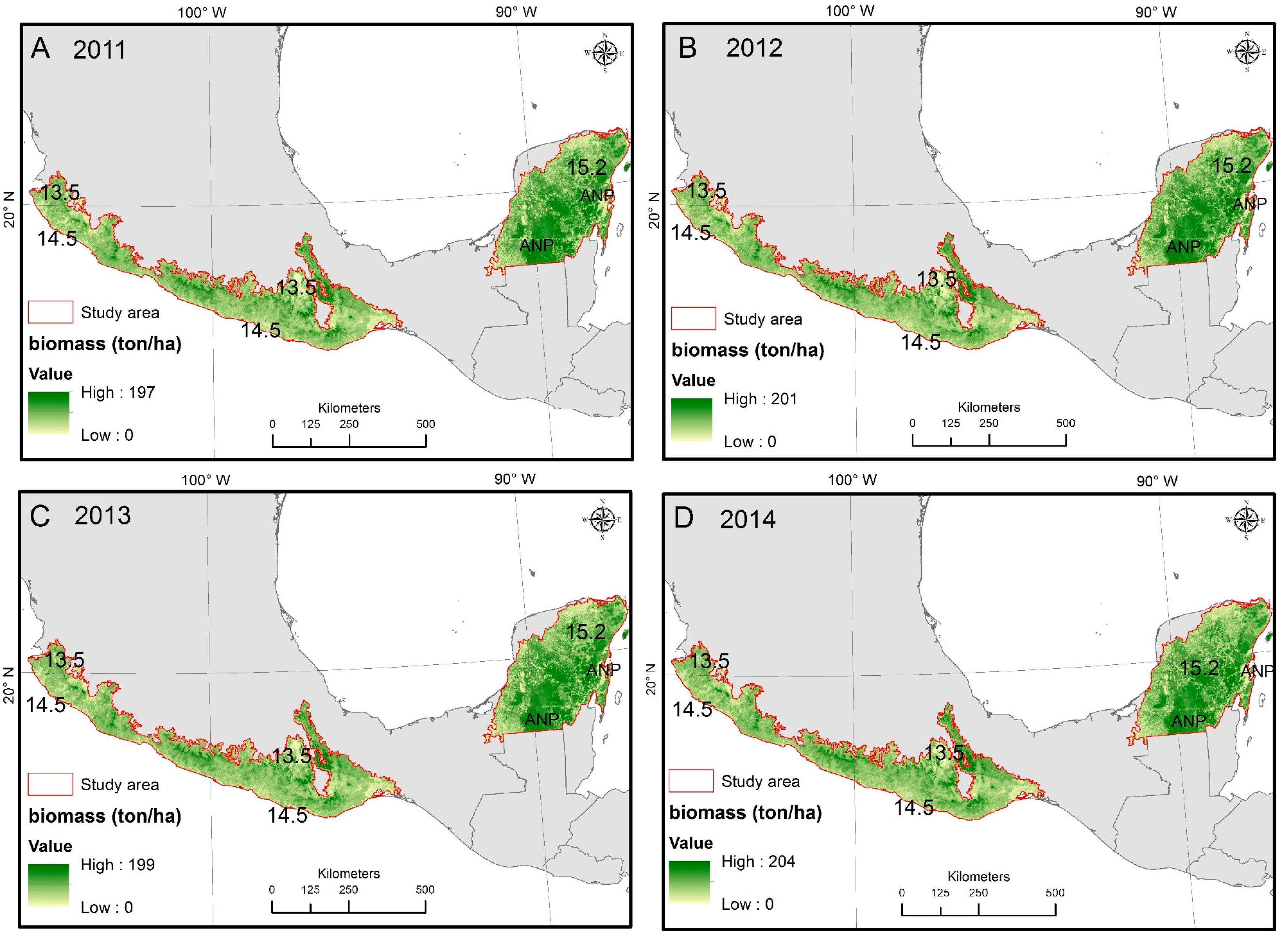
The use of satellite Earth observation data allowed for the spatial and temporal estimation of emissions, providing an annual updating of the biomass and burned areas, as well as the evaluation of environmental conditions for estimating the burning efficiency.
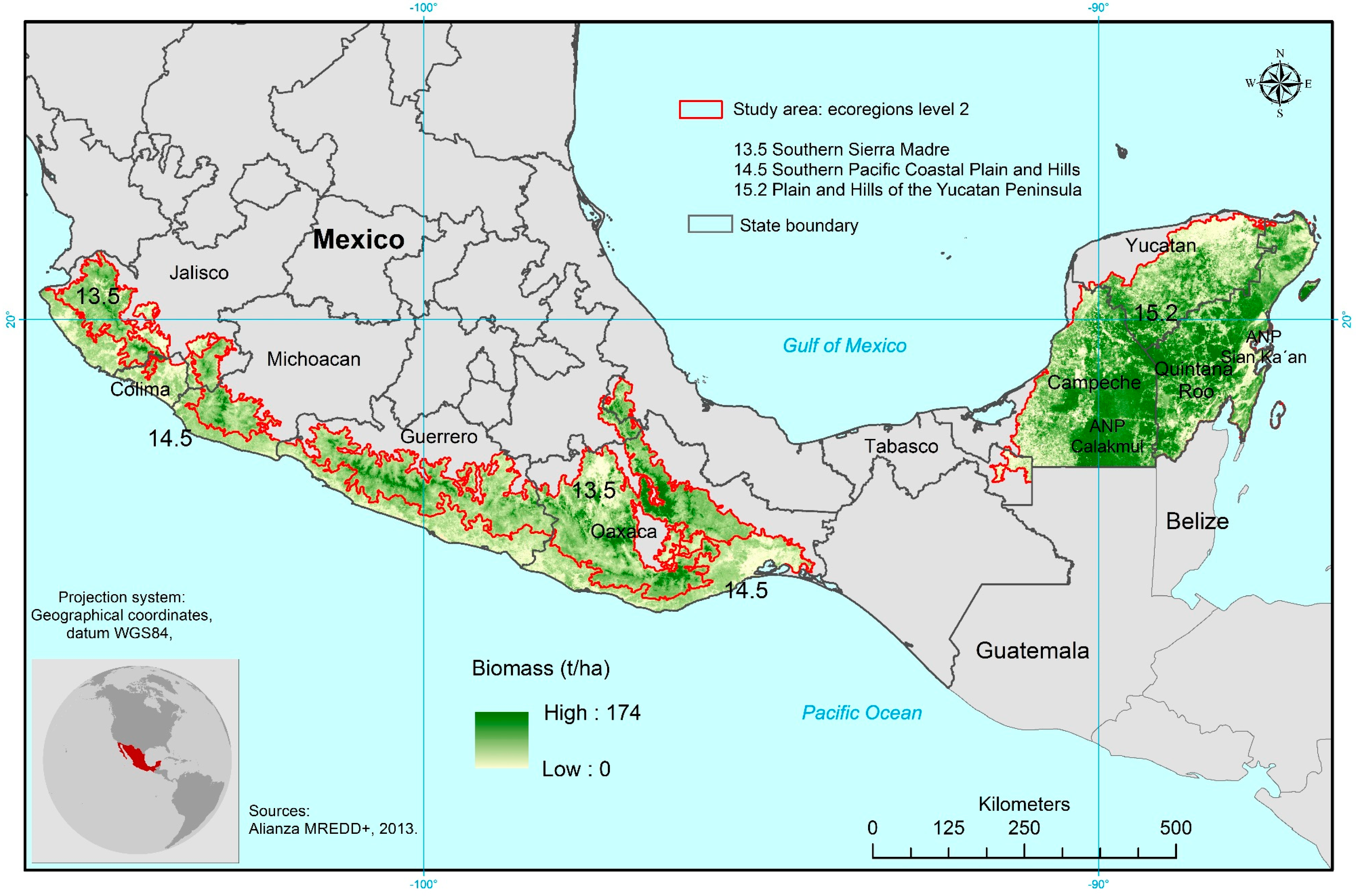
The parameter with the highest uncertainty was the biomass load (27%). Even though the biomass map had an RMSE of 54% in its validation [26], it was still considered acceptable because similar results have been reported by other projects; e.g., the GlobBiomasss project, University of Leicester (2017), reported RMSE values of 51%, 53% and 55% for the years 2005, 2010, and 2015, respectively, in the Central Mexico and Yucatan Peninsula regions. As a complement to the present work, the emissions were estimated by using only the biomass map [26] for each of the four years; this led to a value that was lower by 19 Tg, thereby reinforcing the importance of annual updating.
The burning efficiency results obtained for March 2006 were within those values reported elsewhere: (a) in the literature [50]; (b) in the documentation of prescribed fires [54], and (c) in a study to estimate the spatial variability in burning efficiency in Spain [
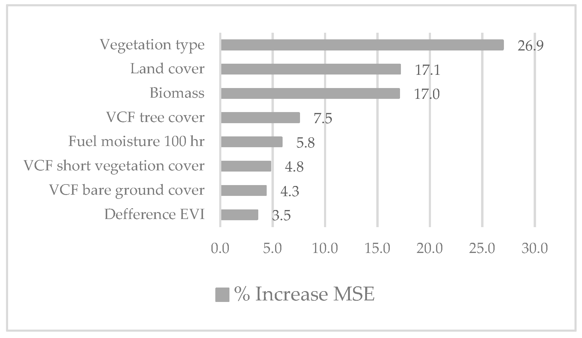
55]. Hence, they were considered appropriate, although they were lower than those reported in the literature. The results also indicated that the behavior of the burning efficiency can be explained by the vegetation type; temperate forests have a relatively low species diversity, and the fire behavior is more uniform than in the species-diverse tropical forests. Here, field data are a fundamental aspect of the method. We considered that the Random Forest approach [36] offers an approximation for estimating the burning efficiency over a large and biodiverse territory such as Mexico; it considers spatial and temporal changes in environmental conditions when a fire occurs, without depending on a unique and static value.
Despite the relatively low accuracy revealed by the omission error for the burned area product, MCD64 has been the best operational product with the historical and recent data, because the data are processed with the same algorithm. This is supported by a study [56] that concluded that the Collection 5.2 MCD64 was the best of three evaluated burned area products, and Collection 6 identifies more burned areas than Collection 5.2.
The emission factors obtained from the MILAGRO project are higher than those reported in the global study of [41] for CO2 and CH4 but lower for CO. These differences have implications in the estimation of emissions because CO2 is the gas with the highest emission factor. However, the MILAGRO data are specific to Mexican vegetation.
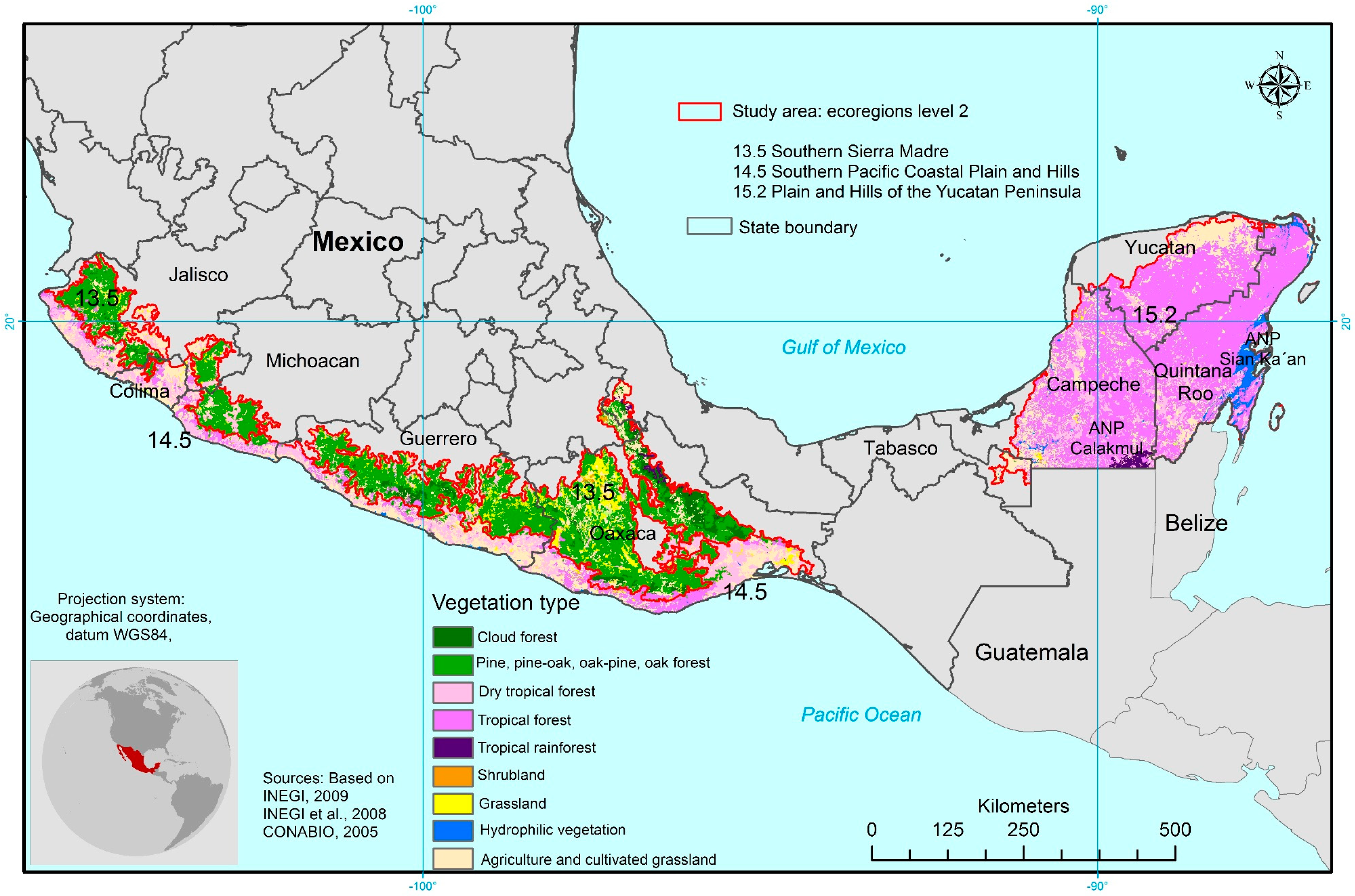
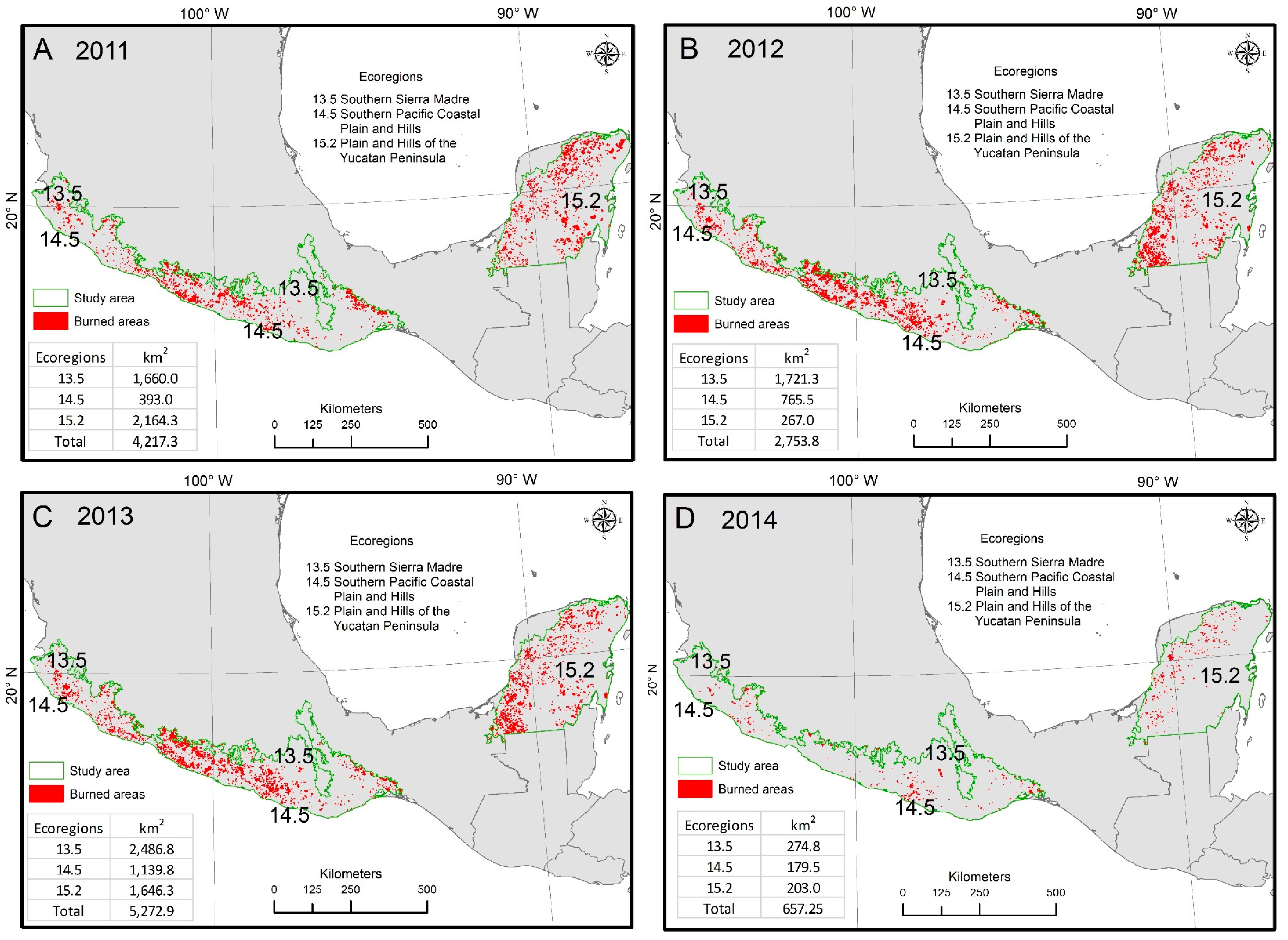
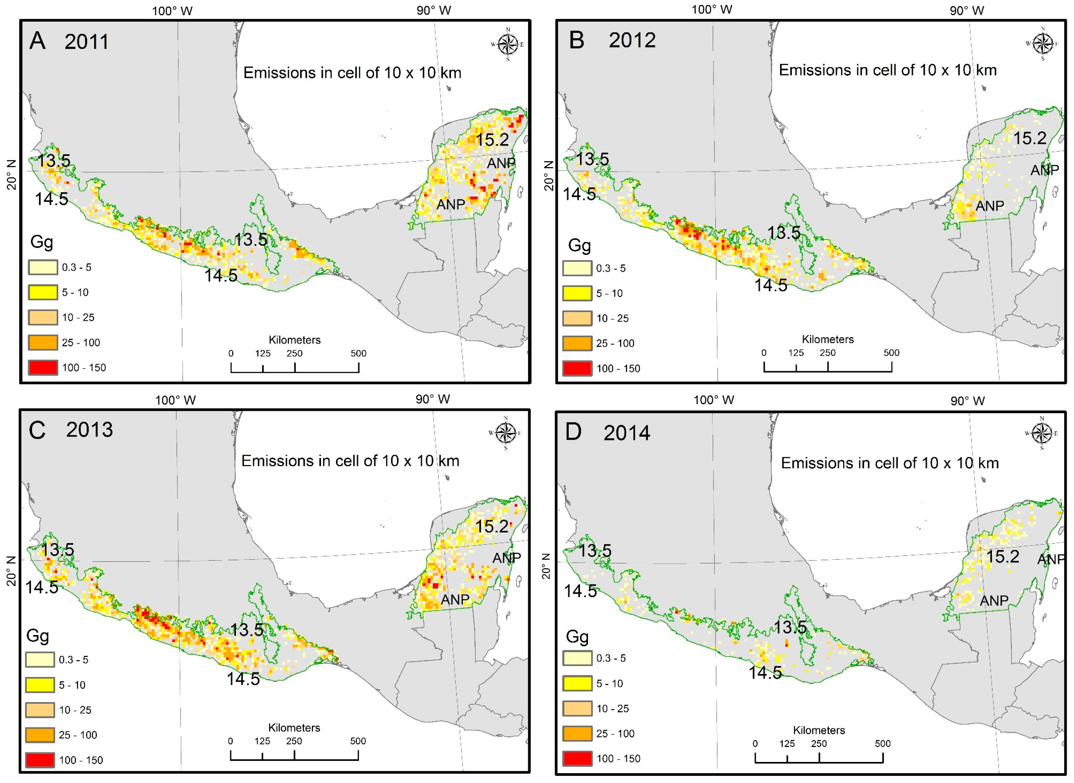
Southern Sierra Madre (ecoregion 13.5) had the highest percentage of emissions, but the vegetation type most affected was the tropical forest distributed in ecoregions 15.2 (Plain and Hills of the Yucatan Peninsula) and 14.5 (Southern Pacific Coastal Plain and Hills). If the emissions originating in temperate forests are added, the result is similar in tropical forests. Therefore, it is important to highlight two elements in the calculation of emissions: the biomass quantity and burning efficiency. Although the amount of emissions per ecoregion reflects the area of that region, it is also influenced by the type of vegetation, the date, and the causes of the fire. For example, ecoregion 13.5 represented 34.8% of the study area and 54.8% of the emissions over the period, whereas ecoregion 15.2 represented 44.3% of the study area but only 28.7% of the emissions.
The differences found between the GFED data and our results are due to the scale of the analysis; GFED is at a global scale without regional detail, giving a general view of the problem, whereas our results have a local precision. We also identified an important difference between our results and a number of previous works [20,21,22]. The results of those three works are similar to each other (9.6 Tg, on average) but lower than those of this study. We found that the burned area parameter had a large influence. CONAFOR statistics recorded less than twice the burned area identified by MCD64A1 Collection 6.0, and this can be explained by the discrepancy in the definition of forest fires. Many fires involving vegetation are associated with the clearing of agricultural fields and with forestry operations; these are not considered uncontrolled fires, and hence are not registered as forest fires, but they are still recorded by MCD64. Hence, it is necessary to identify whether the emissions come from a forest fire or from a change in the land use [57]. Another parameter with an influence on the differences was the biomass. When only the biomass map was considered, without the annual update of NPP, the calculated mean of the emissions fell from 16.8 Tg to 12.1 Tg; even so, this is still a high value.
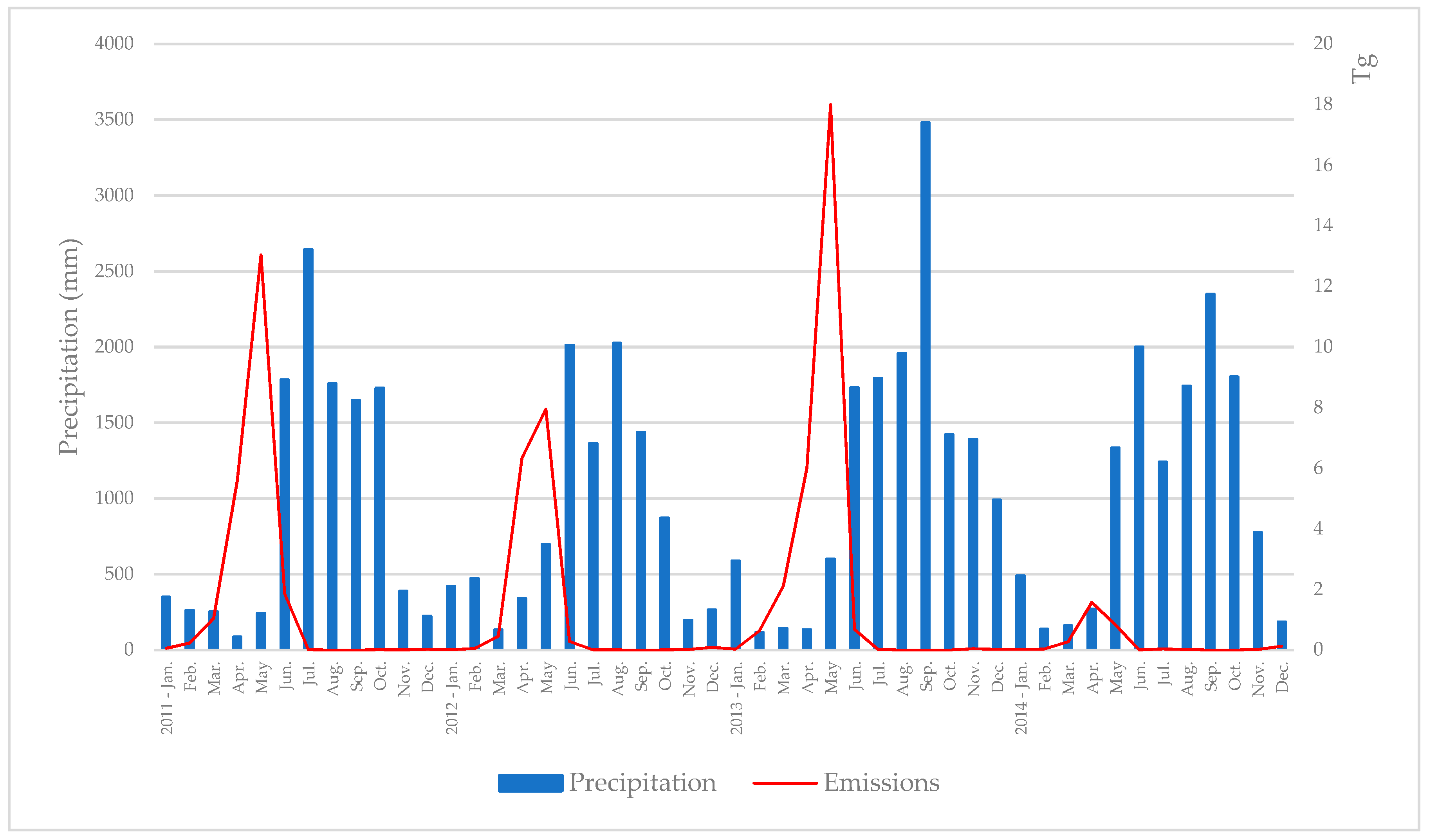
The spatial and temporal distributions of emissions in the study area were associated with the distribution of precipitation, drought, and human activities. There were two very important elements in the emissions distribution: hydrological drought and biomass. The values of the estimated emissions were expected to be low because the estimates of the burning efficiency were small compared with those of other studies. However, the emissions were higher, owing to the inclusion of different inputs, such as a yearly update of the biomass and burned areas. Therefore, it is important to consider the changes over time in the variables and the contribution of satellite data, e.g., the observation of the phenomenon on the day of occurrence. In this work, we considered drought conditions by using the fuel moisture model and the annual update of the biomass.

5. Conclusions

The availability of satellite data and products allows for the estimation and update, both dynamically and periodically, of three out of four parameters for calculating the emissions from forest fires. However, there is still a lack of data with the same resolution and scale to contribute to the precision of the spatial analysis. This was illustrated by a comparison between the GFED data and our results, given that the values of the emissions were very similar, although local discrepancies were observed when data with a better spatial resolution were used.
The present study contributes a product of burned areas that identifies areas affected by fires in vegetation, irrespective of the forest fires registered in the statistics. It is important to collaborate with CONAFOR in using remote sensing data to improve the statistics. Recently, CONAFOR has improved the method for estimating burned areas in the field, and has sometimes incorporated satellite data, in collaboration with CONABIO. Remote sensing data and field knowledge will increase the quality of information regarding emissions. We demonstrated the use of remote sensing data and machine learning to calculate parameters such as the burning efficiency, taking into account natural conditions on the date of the fire; this allows for a better understanding of emissions resulting from forest fires. The areas of interest with burned biomass emissions were located at a larger scale than that used in other works and included an adjustment to the environmental conditions on the date of the fire. This information can help to implement measures to prevent or to mitigate fires according to the environmental characteristics.
The described methodology may be implemented on a countrywide scale because the variables and field data that it uses in the Random Forest Regression (RFR) model are to some degree flexible. As mentioned, it includes an evaluation of the accuracy of its estimates. This allows the methodology to be applied on other ecoregions. Finally, the satellite imagery proposed as input is generated periodically and is available on different distribution platforms.

Author Contributions

M.I.C.-L., L.d.L.M.-D., R.A.-G. and E.C. conceived and designed the proposal; M.I.C.-L. designed and applied the methods and analyzed the results, J.A.E.-B. proposed the use of Random Forest and implemented the calculation of burning efficiency in the R programming language. M.I.C.-L. wrote the paper; L.d.L.M.-D., R.A.-G., E.C. and J.A.E.-B. made corrections.

Funding

This research received no external funding.

Acknowledgments

We thank CONABIO for its data and equipment for processing, German Flores Garnica for his field data to establish the burning efficiency method. René Colditz who provided the time series of vegetation index, and CONABIO for financial assistance for the publication. We thank Ann Grant for corrections to language.

Conflicts of Interest

“The authors declare no conflict of interest.” “The funding sponsors had no role in the design of the study; in the collection, analyses, or interpretation of data; in the writing of the manuscript, and in the decision to publish the results”.

References

  1. Watson, R.T.; Rodhe, H.; Oeschger, H.; Siegenthaler, U. Greenhouse Gases and Aerosol. In Climate Change the IPCC Scientific Assessment; Houghto, J.T., Jekins, G.J., Ephraums, J.J., Eds.; Cambridge University Press: Great Britain, UK, 1990; pp. 7–40. ISBN 0-521-40720-6. [Google Scholar]
  2. Garduño, R. ¿Qué es el efecto invernadero? In Cambio Climático: Una Visión Desde México; Martínez, J., Fernández, A., Eds.; SEMARNAT-INE: Distrito Federal, México, 2004; pp. 29–40. ISBN 968-817-704-0. [Google Scholar]
  3. Álvarez, A. Principios generales del ciclo del carbono en el océano. In Carbono en Ecosistemas Acuáticos de México; Hernández de la Torre, B., Gaxiola, G., Eds.; SEMARNAT-INE-CICESE: Distrito Federal, México, 2007; pp. 11–42. ISBN 978-968-817-855-3. [Google Scholar]
  4. Organización Meteorológica Mundial. Estado del Clima Mundial en 2011–2015; Organización Meteorológica Mundial: Suiza, Switzerland, 2016; pp. 5–9. ISBN 978-92-63-31179-5. [Google Scholar]
  5. Csiszar, I.; Arino, O.; Geraci, R.; Giglio, L.; Goldammer, J.; De Groot, W.; Justice, C.; Kondragunta, S.; Prins, E.; Sessa, R.; Tansey, K. Fire Disturbance Assessment of the Status of the Development of the Standards for the Terrestrial Essential Climate Variables; GTOS: Rome, Italy, 2009; pp. 1–7. [Google Scholar]
  6. GCOS-World Meteorological Organization. The Second Report on the Adequacy of the Global Observing Systems for Climate in Support of the UNFCC—Executive Summary; World Meteorological Organization: Geneva, Switzerland, 2003; pp. 1–4. [Google Scholar]
  7. Levine, J.S. Biomass Burning: The Cycling of Gases and Particulates from the Biosphere to the Atmosphere. In The Atmosphere; Keeling, R., Ed.; Elsevier: Amsterdam, The Netherlands, 2006; pp. 143–158. ISBN 13 978-0-08-045091-9. [Google Scholar]
  8. Whelan, R.J. The Ecology of Fire; Cambridge University Press: Cambridge, UK, 1995; pp. 8–56. ISBN 0-521-33814-X. [Google Scholar]
  9. Roberts, G.; Wooster, M.; Lagoudakis, E. Annual and Diurnal African Biomass Temporal Dynamics. Biogeoscience 2009, 6, 849–866. [Google Scholar] [CrossRef]
  10. Goldammer, J.G.; Statheropoulos, M.; Andreae, M. Impacts of Vegetation Fire Emissions on the Environment, Human Health and Security: A Global Perspective. In Wildland Fires and Air Pollution; Bytnerowicz, A., Arbaugh, M., Riebau, A., Andersen, C., Eds.; Elseiver Science: Amsterdam, The Netherlands, 2009; pp. 3–36. ISBN 978-0-08-055609-3. [Google Scholar]
  11. Seiler, W.; Crutzen, P.J. Estimates of Gross and Net Fluxes of Carbon between the Biosphere and the Atmosphere from Biomass Burning. Clim. Chang. 1980, 2, 207–247. [Google Scholar] [CrossRef]
  12. Wooster, M.J.; Roberts, G.; Perry, G.L. Retrieval of biomass combustion rated and totals from fires radiative power observations: FRP derivation and calibration relationships between biomass consumption and fire radiative energy release. J. Geophys. Res. 2005, 110, 1–24. [Google Scholar] [CrossRef]
  13. van der Werf, G.R.; Randerson, J.T.; Giglio, L.; van Leeuwen, T.T.; Chen, Y.; Rogers, B.M.; Mu, M.; van Marle, M.J.E.; Morton, D.C.; Collatz, G.J.; et al. Global fire emissions estimates during 1997–2016. Earth Syst. Sci. Data 2017, 9, 697–720. [Google Scholar] [CrossRef] [Green Version]
  14. Kaiser, J.W.; Heil, A.; Andreae, M.O.; Benedetti, A.; Chubarova, N.; Jones, L.; Morcrette, J.J.; Razinger, M.; Schultz, M.G.; Suttie, M.; et al. Biomass burning emission estimated with a global fire assimilation system based on observe fire radiative power. Biogeosciences 2012, 9, 527–554. [Google Scholar] [CrossRef]
  15. Wiedinmyer, C.; Quayle, B.; Geron, C.; Belote, A.; McKenzie, D.; Zhang, X.; O´Neill, S.; Wynne, K. Estimating emissions from fires in North America for air quality modeling. Atmos. Environ. 2006, 40, 3419–3432. [Google Scholar] [CrossRef]
  16. Korontzi, S. Seasonal patterns in biomass burning emissions from southern African vegetation fires for the year 2000. Glob. Chang. Biol. 2005, 11, 1680–1700. [Google Scholar] [CrossRef]
  17. Anaya Acevedo, J.A. Estimación Mensual de Emisiones por Biomasa Quemada para Colombia Basado en Imágenes de Satélite. Ph.D. Thesis, Universidad de Alcalá, Alcalá de Henares, España, 2009. [Google Scholar]
  18. CONAFOR. Programa Nacional de Prevención de Incendios forestales; Comisión Nacional Forestal: Jalisco, México, 2015. [Google Scholar]
  19. Ben de Jong; Olguín, M.; Rojas, F.; Maldonado, V.; Paz, F.; Etchever, J.; Cruz, C.O.; Abad, J.A. Actualización del Inventario Nacional de Emisiones de Gases de Efecto Invernadero 1990–2006 en la Categoría de Agricultura, Silvicultura y otros Usos de la Tierra; Instituto de Ecología: Distrito Federal, México, 2006; pp. 93–94. [Google Scholar]
  20. Bautista, F.; Carbajal, N.; Pineda, L.F. Estimation of Total Yearly CO2 Emissions by Wildfires in Mexico during the Period 1999–2010. Adv. Meteorol. 2014, 2014, 1–8. [Google Scholar] [CrossRef]
  21. CONAFOR. Propuesta del Nivel de Referencia de las Emisiones Forestales de México; Comisión Nacional Forestal-SEMARNAT: Jalisco, México, 2014. [Google Scholar]
  22. INECC—SEMARNAT. Primer Informe Bienal de Actualización ante la Convención Marco de las Naciones Unidas sobre el Cambio Climático; INECC/SEMARNAT: Distrito Federal, México, 2015; pp. 88–92. [Google Scholar]
  23. INEGI-CONABIO-INE. Ecorregiones Terrestres de México; Escala 1:1,000,000; INEGI-CONABIO-INE: Distrito Federal, México, 2008. [Google Scholar]
  24. Sistema de Alerta Temprana de Incendios Forestales. Available online: http://incendios.conabio.gob.mx/ (accessed on 22 August 2014).
  25. Chuvieco, E. Satellite Observation of Biomass Burning. In Earth Observation of Global Change, The Role of Satellite Remote Sensing in Monitoring the Global Environment; Chuvieco, E., Ed.; Springer: New York, NY, USA, 2008; pp. 109–142. ISBN 978-1-4020-6357-2. [Google Scholar]
  26. Alianza MREDD. Mapa y Base de Datos sobre la Distribución de la Biomasa aérea de la Vegetación Leñosa en México; Versión 1.0; Woods Hole Research Center, USAID, CONAFOR, CONABIO, Proyecto México-Noruega: Zapopan, México, 2013. [Google Scholar]
  27. Cartus, O.; Kellndorfer, J.; Walker, W.; Franco, C.; Bishop, J.; Santos, L.; Michael Fuentes, J.M. A National Detailed Map of Forest Aboveground Carbon Stocks in Mexico. Remote Sens. 2014, 6, 5559–5588. [Google Scholar] [CrossRef]
  28. Morfín Ríos, J.E.; Michael, J.M.; González, R.; Carrillo, O.; Mayorga, R.; Rangel, L.; Orozco, J.; Rodríguez, G.; Guerrero, G. Protocolo Estimaciones de las Reservas del Carbono en la Biomasa Forestal en México; Gobierno de Noruega Ministerio de Asuntos Internacionales—CONAFOR—PNUD, FAO: Jalisco, México, 2015; pp. 46–54. [Google Scholar]
  29. Lieth, H. Primary Production of the Major Vegetation Units of the World. In Primary Productivity of the Biosphere; Lieth, H., Whittaker, R.H., Eds.; Springer: Heidelberg, Germany, 1975; pp. 203–215. ISBN 978-3-642-80915-6. [Google Scholar]
  30. Whittaker, R.H.; Marks, P.L. Methods of Assessing Terrestrial Productivity. In Primary Productivity of the Biosphere; Lieth, H., Whittaker, R.H., Eds.; Springer: New York, NY, USA, 1975; pp. 55–118. ISBN 978-3-642-80915-6. [Google Scholar]
  31. MODIS GPP/NPP Project (MOD17). Available online: http://www.ntsg.umt.edu/project/modis/mod17.php (accessed on 11 March 2015).
  32. Ramo, R.; Chuvieco, E. Developing a Random Forest Algorithm for MODIS Global Burned Area Classification. Remote Sens. 2017, 9, 1193. [Google Scholar] [CrossRef]
  33. Colditz, R.R.; Lopez Saldaña, G.; Maeda, P.; Argumedo Espinoza, J.; Meneses Tovar, C.; Victoria Hernandez, A.; Zermeño Benitez, C.; Cruz Lopez, M.I.; Ressl, R. Generation and analysis of the 2005 land cover map for Mexico Using 250m Modis data. Remote Sens. Environ. 2012, 123, 541–552. [Google Scholar] [CrossRef]
  34. Cervera Taboada, A. Implementación de un Modelo para Estimar la Humedad del Combustible Muerto Basado en datos de Sensores Remotos. Ph.D. Thesis, Universidad Nacional Autónoma de México, Distrito Federal, México, 2009. [Google Scholar]
  35. Murray, F.W. On the computation of saturation vapor pressure. J. Appl. Meteorol. Climatol. 1967, 6, 203–204. [Google Scholar] [CrossRef]
  36. Cruz López, M.I. Una Aproximación para estimar la eficiencia del quemado usando productos satelitales, caso de estudio: México. Geofocus 2018, 21, 119–143. [Google Scholar] [CrossRef]
  37. Roy, D.; Boschetti, L.; Justice, C.O. The Global MODIS Burned Area Products. In Proceedings of the IV Conferencia internacional sobre incendios forestales, Sevilla, España, 13–18 May 2007. [Google Scholar]
  38. Roy, D.; Jin, Y.; Lewis, P.E.; Justice, C.O. Prototyping a Global Algorithm for Systematic Fire-Affected Area Mapping Using MODIS Time Series Data. Remote Sens. Environ. 2005, 97, 137–162. [Google Scholar] [CrossRef]
  39. Giglio, L.; Loboda, T.; Roy, D.; Quayle, B.; Justice, C. An Active-fire Based Burned Area Mapping Algorithm for the MODIS Sensor. Remote Sens. Environ. 2009, 113, 408–420. [Google Scholar] [CrossRef]
  40. Boschetti, L.; Roy, D.P.; Justice, C.O. International Global Burned Areas Satellite Products Validation Protocol. Part I Production and Standardization of Validation Reference Data. Available online: https://bit.ly/2Es6rqT (accessed on 18 May 2019).
  41. Andreae, M.O.; Merlet, P. Emission of Trace Gases and Aerosols from Biomass Burning. Glob. Biogeochem. Cycles 2001, 15, 955–966. [Google Scholar] [CrossRef]
  42. Yokelson, R.J.; Burling, I.R.; Urbanski, S.P.; Atlas, E.L.; Adachi, K.; Buseck, P.R.; Wiedinmayer, C.; Akagi, S.K.; Toohey, D.W.; Wold, C.E. Trace Gas and Particle Emissions from Open Biomass in Mexico. Atmos. Chem. Phys. 2011, 11, 6787–6808. [Google Scholar] [CrossRef]
  43. Urbanski, S. Wildland Fire Emissions, Carbon and Climate: Emission Factors. For. Ecol. Manag. 2014, 317, 51–60. [Google Scholar] [CrossRef]
  44. Monni, S.; Herold, M.; Grassi, G.; Brown, S.; McRoberts, R.E. Estimation of Uncertainties. In A Sourcebook of Methods and Procedures for Monitoring and Reporting Anthropogenic Greenhouse Gas Emissions and Removals Associated with Deforestation, Gains and Losses of Carbon Stocks in Forest Remaining Forest, and Forestation; GOFC-GOLD, Land Cover Project Office Wageningen University: Wageningen, The Netherlands, 2016. [Google Scholar]
  45. Congalton, R.G.; Green, K. Assessing the Accuracy of Remotely Senses Data; CRC Press Taylor & Francis Group: Boca Ratón, FL, USA, 2008; pp. 55–104. ISBN 978-1-4200-5512-2. [Google Scholar]
  46. Giglio, L.; Randerson, J.T.; van der Werf, G.R. Analysis of Daily, Monthly and Annual Burned Area Using the Fourth-Generation Global Fire Emissions Database (GFED4). J. Geophys. Res. 2013, 118, 317–328. [Google Scholar] [CrossRef]
  47. Randerson, J.T.; Chen, Y.; van der Werf, G.R.; Roger, B.M.; Morton, D.C. Global Burned Area and Biomass Burning Emissions from Small Fire. J. Geophys. Res. 2012, 117, 1–23. [Google Scholar] [CrossRef]
  48. Van der Werf, G.; Randerson, J.; Giglio, L.; Collatz, G.; Mu, M.; Kasibhatla, P.; Morton, D.; De Fries, R.; Jin, Y.; Van Leeuwen, T. Global Fire Emissions and the Contribution of Deforestation, Savanna, Forest, Agricultural, and Peat Fires (1997–2009). Atmos. Chem. Phys. 2010, 10, 11707–11735. [Google Scholar] [CrossRef]
  49. Meinshausen, N. Quantile Regression Forest. J. Mach. Learn. Res. 2006, 7, 983–999. [Google Scholar]
  50. CONAFOR. Manual de Información de Resultados en Incendios Forestales; Comisión Nacional Forestal, Zapopan: Jalisco, México, 2014; pp. 12–13. [Google Scholar]
  51. Monitoreo de sequía de América del Norte 2011. Available online: http://smn.cna.gob.mx/es/climatologia/monitor-de-sequia/monitor-de-sequia-de-america-del-norte (accessed on 25 May 2017).
  52. Monitoreo de sequía de América del Norte 2012. Available online: http://smn.cna.gob.mx/es/climatologia/monitor-de-sequia/monitor-de-sequia-de-america-del-norte (accessed on 25 May 2017).
  53. Precipitación a Nivel Nacional y por Entidad Federativa. 2011, 2012. 2013, 1014. Available online: http://smn.cna.gob.mx/tools/DATA/Climatolog%C3%ADa/Pron%C3%B3stico%20clim%C3%A1tico/Temperatura%20y%20Lluvia/PREC/ (accessed on 24 March 2017).
  54. Rodríguez Trejo, D.A. Incendios de Vegetación, su Ecología, Manejo e Historia; Biblioteca básica de agricultura: Chapingo, México, 2014; pp. 103–790. ISBN 978-607-715-237-8. [Google Scholar]
  55. Oliva, P.; Chuvieco, E. Estimación de la eficiencia del quemado a partir de la severidad de quemado. In Teledetección, Bosque y Cambio Climático, Proceedings of XIV Congreso de la Asociación Española de Teledetección, Universidad de Oviedo, España, 21 al 23 de septiembre de 2011; Recondeo-González, C., y Pendás-Molina, E., Eds.; Asociación Española de Teledetección: Oviedo, España, 2011. [Google Scholar]
  56. Padilla, M.; Stehman, S.V.; Hantson, S.; Oliva, P.; Alonso-Canas, I.; Bradley, A.; Tansey, K.; Mota, B.; Pereira, J.M.; Chuvieco, E. Comparing the Accuracies of Remote Sensing Global Burned Area Products using Stratified Random Sampling and Estimation. Remote Sens. Environ. 2015, 160, 114–121. [Google Scholar] [CrossRef]
  57. Jardel, E.; (Universidad de Guadalajara, Autlán, Jalisco, México). Personal communication, 2018.
Figure 1. Study area: three selected ecoregions.
Remotesensing 11 01185 g001
Figure 2. Biomass map (Alianza MREDD + (Mexico Reducing Emissions from Deforestation and forest Degradation plus, 2013).
Remotesensing 11 01185 g002
Figure 3. Annual updated biomass. A: 2011; B: 2012; C: 2013; D: 2014.
Remotesensing 11 01185 g003
Figure 4. Variable importance.
Remotesensing 11 01185 g004
Figure 5. Burned areas from 2011-2014. A: 2011; B: 2012; C: 2013; D: 2014.
Remotesensing 11 01185 g005
Figure 6. Emissions from forest fires in three ecoregions in Mexico. A: 2011; B: 2012; C: 2013; D: 2014.
Remotesensing 11 01185 g006
Figure 7. Precipitation and emissions from fires in the study regions.
Remotesensing 11 01185 g007
Figure 8. Areas of interest in terms of forest fire emissions in three ecoregions of Mexico.
Remotesensing 11 01185 g008
Table 1. Biomass map and biomass from the NPP correlation 1.
Biomass Alianza mapBiomass NPP 2011Biomass NPP 2012Biomass NPP 2013Biomass NPP 2014
Biomass Alianza map1.00000.81740.83200.81800.8176
Biomass NPP 20110.81741.00000.99560.99500.9608
Biomass NPP 20120.83200.99561.00000.99490.9641
Biomass NPP 20130.81800.99500.99491.00000.9639
Biomass NPP 20140.81760.96080.96410.96391.0000
1 The correlation was calculated using ENVI (Environment for Visualizing Images) software. NPP: Net Primary Productivity.
Table 2. Estimated burning efficiency and literature data.
PFOFPOFOPFDTFTFGCF
Estimated
Minimum0.500.470.420.500.370.410.390.46
Mean0.510.570.480.540.470.500.450.49
Maximum0.520.610.520.600.550.590.530.52
CONAFOR0.750.710.740.740.960.5s/d0.81
PF: pine forest, OF: oak forest, POF: pine-oak forest, OPF: oak-pine forest, DTF: dry tropical forest, TF: tropical forest, G: grassland, CF: cloud forest. CONAFOR: Comisión Nacional Forestal.
Table 3. Emissions factors (g/kg).
Original Reference Vegetation Type (INEGI)CO2CONOxCH4NH3PM2.5
Temperate forest 1Pine forest1638100.751.9104.4130.91816.94
Pine-oak forest 2Oak forest1603102.903.6585.7040.51811.33
Pine-oak forest1603102.903.6585.7040.51811.33
Oak-pine forest1603102.903.6585.7040.51811.33
Cloud forest1603102.903.6585.7040.51811.33
Tropical dry forest 2Tropical dry forest165787.134.6255.6812.4774.50
Tropical forest165787.134.6255.6812.4774.50
Savanna 2Grassland166079.286.0314.1260.4777.65
Shrubland 1Shrubland167474.002.1803.6901.5007.06
Hydrophilic vegetation165787.134.6255.6812.4774.50
1 Urbanski (2014). We used mean values in the forest case. 2 Yokelson et al. (2011). Mean values were used.
Table 4. Emissions reported in the study area by ecoregion in Tg.
YearSouthern Sierra Madre (13.5)Southern Pacific Coastal Plain and Hills (14.5)Plain and Hills of the Yucatan Peninsula (15.2)Total
20119.61.610.721.9
201210.93.11.215.2
201314.85.07.727.5
20141.40.60.92.9
Table 5. Emissions by vegetation type.
Vegetation Type2011 (%)2012 (%)2013 (%)2014 (%)
Pine forest2.59.75.83.8
Oak Forest10.414.816.514.1
Pine- oak forest 19.223.817.711.6
Oak- pine forest3.814.09.67.2
Cloud forest4.34.92.72.8
Dry tropical forest8.214.311.617.4
Tropical forest46.711.729.430.8
Tropical rainforest0.50.10.30.0
Grassland3.75.95.912.0
Hydrophilic vegetation0.81.00.40.3
100100100100
Table 6. Areas of interest by forest fire emissions.
EcoregionStateIdNameTotal Emissions (Tg)Cell Area (Km2)
13.5GuerreroAWestern Guerrero State12.434300
GuerreroBCentral Guerrero State4.232000
OaxacaCSierra Juarez1.00700
15.2Quintana RooDSite between Sian Ka´an and Calakmul3.471600
Quintana RooECancun1.721000
CampecheFSite between Calakmul and Laguna de Terminos1.59900
Table 7. Emissions of carbon (Tg).
YearCarbon Estimated in Burned Areas in Vegetation Carbon Estimated by GFED in All ClassesCarbon Estimated by GFED in Forest AreaCorrelation 1 (r2)
20116.112.17.00.52
20124.33.30.80.11
20137.713.57.80.12
20140.81.80.30.24
1 Polynomial correlation. We considered all cells of 10 × 10 km. GFED: Global Fire Emissions Database.

