Arctic Vegetation Mapping Using Unsupervised Training Datasets and Convolutional Neural Networks
by
 , ,
, ,
Zachary L. Langford
1,2,*, 
Jitendra Kumar
1,2,
Forrest M. Hoffman
3,4 ,
,
Amy L. Breen
5 and
Colleen M. Iversen
1,2 1
Bredesen Center for Interdisciplinary Research and Graduate Education, University of Tennessee, Knoxville, TN 37996, USA
2
Environmental Sciences Division, Oak Ridge National Laboratory, Oak Ridge, TN 37831, USA
3
Computational Sciences and Engineering Division, Oak Ridge National Laboratory, Oak Ridge, TN 37831, USA
4
Department of Civil and Environmental Engineering, University of Tennessee, Knoxville, TN 37996, USA
5
International Arctic Research Center, University of Alaska, Fairbanks, AK 99775, USA
*
Author to whom correspondence should be addressed.
Remote Sens. 2019, 11(1), 69; https://doi.org/10.3390/rs11010069
Submission received: 1 November 2018
/
Revised: 15 December 2018
/
Accepted: 25 December 2018
/
Published: 2 January 2019
(This article belongs to the Special Issue Machine Learning Applications in Earth Science Big Data Analysis)
Abstract
:Land cover datasets are essential for modeling and analysis of Arctic ecosystem structure and function and for understanding land–atmosphere interactions at high spatial resolutions. However, most Arctic land cover products are generated at a coarse resolution, often limited due to cloud cover, polar darkness, and poor availability of high-resolution imagery. A multi-sensor remote sensing-based deep learning approach was developed for generating high-resolution (5 m) vegetation maps for the western Alaskan Arctic on the Seward Peninsula, Alaska. The fusion of hyperspectral, multispectral, and terrain datasets was performed using unsupervised and supervised classification techniques over a ∼343 km2 area, and a high-resolution (5 m) vegetation classification map was generated. An unsupervised technique was developed to classify high-dimensional remote sensing datasets into cohesive clusters. We employed a quantitative method to add supervision to the unlabeled clusters, producing a fully labeled vegetation map. We then developed convolutional neural networks (CNNs) using the multi-sensor fusion datasets to map vegetation distributions using the original classes and the classes produced by the unsupervised classification method. To validate the resulting CNN maps, vegetation observations were collected at 30 field plots during the summer of 2016, and the resulting vegetation products developed were evaluated against them for accuracy. Our analysis indicates the CNN models based on the labels produced by the unsupervised classification method provided the most accurate mapping of vegetation types, increasing the validation score (i.e., precision) from 0.53 to 0.83 when evaluated against field vegetation observations.
1. Introduction
Alaska is experiencing warmer temperatures and increased precipitation, with substantial spatial variability [1,2]. These environmental variations could have considerable consequences for terrestrial ecosystems, such as Arctic plant communities [3]. Vegetation changes across Alaska will also have potential implications for carbon cycling [4], rates of evapotranspiration [5], permafrost dynamics [6,7], and fire regimes [8,9]. Therefore, accurate and up-to-date vegetation maps are essential in Alaska for ecosystem studies.
High-resolution and accurate vegetation datasets are needed for current climate modeling projects in Alaska, such as the Next-Generation Ecosystem Experiments (NGEE Arctic) (http://ngee-arctic.ornl.gov/). NGEE Arctic is modeling Arctic climate change at a variety of scales and also includes associated feedbacks to climate [10,11]. It is important to evaluate remote sensing imagery that can provide datasets to drive high-resolution models and guide field sampling campaigns. For example, Langford et al. 2016 [12] used WorldView-2 and LiDAR datasets to create ∼0.25 m spatial resolution plant functional type (PFT) datasets for driving land-surface models in Utqiagvik, AK.
Satellite remote sensing is a complementary tool for monitoring natural and anthropogenic temporal and spatial changes in these environments; however, cloud cover, polar darkness, and a sparse number of publicly available high-resolution datasets are limiting factors [13]. High-resolution (∼0.3–10 m) multispectral datasets (e.g., IKONOS, QuickBird, SPOT, and WorldView) are becoming more available in Arctic and Boreal ecosystems. Other coarse multispectral satellite sensors, such as Landsat, have extensive coverage over Alaska and are shown to be effective for Arctic vegetation mapping over large areas [14,15]. Additionally, other imaging modalities are becoming more accessible, such as hyperspectral datasets. Analysis based on hyperspectral imagery and measurements have shown to be effective for identification of Arctic vegetation types [16,17].
Sensor fusion is a way of combining measurements from different sources to obtain a result that is in some sense better than what could have been achieved without this combination [18]. For example, the detailed spectral and spatial information provided by multi/hyperspectral imagery increases the power of accurately differentiating materials of interest [19]. It is imperative to find optimal machine learning algorithms (i.e., supervised and unsupervised classifications) that can make use of multisensor fusion datasets across Alaska.
Sparse and missing datasets for training classification algorithms are common in remote sensing applications. This is especially common when collecting vegetation datasets in the field, which for low stature vegetation in the Arctic are typically from plots with an area <5 m2. There is a need to develop accurate training datasets for classification. Unsupervised classification approaches are efficient for grouping pixels with common characteristics of multi-variate datasets; however, they are unlabeled and thus are often hard to analyze and validate. There have been approaches that use simple quantitative scores to label datasets based on unsupervised clustering [20]. For example, Bond-Lamberty et al. [21] used goodness-of-fit and k-means clustering to compare clusters with global International Geosphere–Biosphere Programme (IGBP) Land Cover Classification for creating Decomposition Functional Type maps.
Convolutional Neural Networks (CNNs) are artificial neural networks that learn spatial-contextual features in several hierarchical nonlinear layers [22], and have been shown to provide good performance for image classification in the remote sensing community [23]. CNNs have also been shown to be effective on multi/hyperspectral imagery and sensor fusion for classification tasks [24,25,26]. However, most approaches using CNNs on multi/hyperspectral imagery use coarse spatial resolution (e.g., 30 m) datasets at small spatial scales (e.g., Indian Pines, Salinas, etc.). Additionally, there often is a lack of ground-truth data collected in the field for validation.
In this study, we develop a multisensor remote sensing fusion approach for high-resolution mapping of vegetation in Arctic Alaska. This paper contributes to the remote sensing community by applying an unsupervised approach for generating training datasets for supervised classification approaches (e.g., CNNs) to improve vegetation classification for field-scale products. We believe that the publicly available data (Alaskan Existing Vegetation Type (AKEVT) map) over our study region is inaccurate at the field-scale level (e.g., <2 km2), since this was prepared for a large extent of Alaska using coarse datasets (i.e., Landsat 7). Specifically, we apply unsupervised classification (k-means clustering) and use a quantitative method to add labels to the clusters. This is done to improve spatial resolution (i.e., 30 m to 5 m) and reduce noise in a publicly available vegetation dataset over the region for creating training datasets. Two CNN models were built using original and updated vegetation maps for training to classify the multisensor dataset. We then evaluate the CNN vegetation maps using 30 field plots.
The paper is structured as follows: Section 2 describes the study area; Section 3.1 provides a description of the remote sensing datasets used in the study and the data processing performed; Section 3.2 describes the unsupervised classification of remote sensing datasets and method for assigning vegetation class labels; Section 3.3 describes the CNN-based supervised classifications; Section 3.4 describes validation of the CNN-based vegetation maps using (a) validation dataset held out from training set; and (b) field plot datasets collected at our study sites. Section 4 describes the results and Section 5 provides discussion of the results. Section 6 provides the conclusion of the study, highlights the key contributions, and discusses the limitations of multisensor fusion for high-resolution vegetation mapping at the field-scale.
2. Study Area
The study region (SR) is located on the Seward Peninsula on the western coast of Alaska (Figure 1). The Seward Peninsula experiences a semi-maritime climate controlled by the Bering Sea and sea surface conditions [27]. The Seward Peninsula hosts a variety of vegetation types (e.g., short- and tall-statured shrubs, grasses, sedges, forbs, lichens and mosses) and includes a transition from boreal forest to tundra [28]. The bounding perimeter of the study region was determined by the overlapping raster boundaries from the source imagery. Additional details are contained in Section 3.1.
This study was focused at a watershed in the middle of the Seward Peninsula (Figure 1), where intensive field campaigns to study hydrology, biogeochemistry, and vegetation are being conducted by the NGEE Arctic project. The Kougarok watershed (KW) (65°09′44″ N, 164°49′07″ W) has an area of 1.75 km2 and consists of low Arctic tundra dominated by open low Mixed Shrub-Sedge Tussock Tundra communities [29]. The mean annual temperature around Kougarok is −2.4 °C and the mean annual temperature in July is 11.0 °C, while the mean annual precipitation is 102.1 mm [30]. The Kougarok area is a zone of nearly continuous permafrost with an active layer that has a mean thickness of 56 cm [31].
3. Materials and Methods
The methods section follows the structure shown in Figure 2. Section 3.1 discusses the geospatial datasets used in this study and how they were acquired and processed. Section 3.2 discusses the stratification of landscape using unsupervised clustering and how vegetation labels were assigned to the clusters. Additionally, this section describes how the the labels were generated for training the CNN using unsupervised methods. Section 3.3 discusses the CNN based supervised classification approach using the unsupervised classification based vegetation map for training. Section 3.4 discusses the validation statistics across the entire study region and use of field data for validation.
3.1. Geospatial and In Situ Datasets
This section describes how the datasets were collected and processed. Datasets derived from EO-1 Hyperion, Landsat 8 OLI, Satellite for Observation of Earth (SPOT-5), and a Digital Surface Model (DSM) based on Interferometric Synthetic Aperture Radar (IfSAR) were used. The fusion of datasets was performed by stacking multiple bands together and re-sampled using nearest-neighbor interpolation and pixel aggregation to 5 m. Additionally, the AKEVT map was re-sampled to 5 m using the same method. We chose to focus on the combination of EO-1 Hyperion, SPOT-5, Landsat 8, and IfSAR DSM. This was based on the analysis performed by Langford et al. 2017 [24].
The EO-1 Hyperion and Landsat 8 OLI images were collected from USGS (https://earthexplorer.usgs.gov/), with EO-1 Hyperion consisting of 198 calibrated bands (0.4–2.5 μm), with the non-calibrated bands removed, and Landsat 8 OLI consisting of 11 bands, with 9 bands (0.4–2.29 μm) used in this study. Both datasets were terrain corrected (e.g., Level 1Gst for EO-1) and radiometrically-corrected. The EO-1 Hyperion and Landsat 8 OLI datasets were converted to Top Of Atmosphere (TOA) reflectance according to the USGS documentation. Please see https://landsat.usgs.gov/using-usgs-landsat-8-product for Landsat 8 processing and https://archive.usgs.gov/archive/sites/eo1.usgs.gov/hyperion_documents.html for EO-1 Hyperion.
The DSM and SPOT-5 data were collected from the Geographic Information Network of Alaska (http://gina.alaska.edu/). The 30 m Alaska Existing Vegetation Type (AKEVT; http://akevt.gina.alaska.edu/) vegetation map was acquired and clipped to the study region. The AKEVT map consisted of six main vegetation classes for the study region based on an aggregation of the Alaska Vegetation Classification [29]. Table 1 shows the area distribution of the AKEVT vegetation classes present in the study region and a crosswalk to the other sources used in field data preparation.
All datasets were processed in Alaska Albers Equal Area Conic (EPSG:3338), NAD83 horizontal datum and NAVD88 vertical datum. The SPOT-5 satellite images used in this study were collected by the “Alaska Statewide Digital Mapping Initiative”, which produced a new statewide orthomosaic that provides complete multispectral coverage of the state at 2.5 m spatial resolution. The SPOT-5 orthoimage used to create the digital orthoimages were acquired between 2009 and 2013. Three statewide mosaics are available: color infrared (CIR), psuedo-natural color, and panchromatic (grayscale). The CIR SPOT-5 orthoimage was used over the study area, which consists of the green (0.50–0.59 μm), red (0.61–0.68 μm), and near infrared (0.78–0.89 μm) bands. Quantum Spatial and Fugro Geospatial, Inc. performed the image processing, orthorectification, and mosaicing of the datasets. The Alaska Statewide Digital Mapping Initiative (http://www.alaskamapped.org/ortho) has more details on the image processing for the SPOT-5 orthoimage. The SPOT-5 and DSM datasets were normalized to be between 0 and 1 for consistency among the TOA datasets (Landsat 8 and EO-1 Hyperion). This was performed by:
where x = (, …, ) are the Digital Numbers (DN) values of the datasets and is the the normalized data. Table 2 shows the image dates, variables, and resolution.
Some vegetation classes had small presence (by area) within our study area and thus were merged into other classes of similar strata. This was done based on the Alaska vegetation classification system [29]. For example, the Willow Shrubs classification covered only 0.38% of the study region and was merged into the Alder-Willow Shrub class. Six primary vegetation types were mapped in the study region: (1) Alder-Willow Shrub, (2) Mixed Shrub-Sedge Tussock Tundra-Bog, (3) Dryas/Lichen Dwarf Shrub Tundra, (4) Sedge-Willow-Dryas Tundra, (5) Non-Vegetated (i.e., snow-ice, rock, sand, gravel), and (6) Water.
Sampling of vegetation plots in the field utilized methods recommended for the Arctic region by the authors of the Arctic Vegetation Archive prototype for northern Alaska [32]. Vegetation plots were selected in areas of homogenous vegetation. Field sampling of plots included: (1) complete vascular plant, bryophyte, and lichen species lists and their percent cover, (2) percent cover and mean height of each plant functional group, (3) site description, and (4) permanent marking and geo-referencing of plots. All plots were classified with respect to the Alaska Arctic Tundra Vegetation Map (AATVM) [33] for the following vegetation types: Willow-Birch Tundra, Alder Shrubland, Tussock Tundra, Shrubby Tussock Tundra or Alder Savanna, Dwarf Shrub Lichen Tundra, and Non-acidic Mountain Complex. These vegetation types were crosswalked to the AKEVT map resulting in three main classes of vegetation including Mixed Shrub-Sedge Tussock Tundra-Bog, Dryas/Lichen Dwarf Shrub Tundra, and Alder-Willow Shrub. Table 1 shows the crosswalk, number of plots, and the size of field plots by vegetation type.
3.2. Unsupervised Classification Based Vegetation Mapping (UCVM)
A k-means algorithm was used for stratification of the landscape using remote sensing datasets (Table 2). The k-means algorithm clusters a dataset (, , …, ) with n records into a desired number of clusters, k, equalizing the full multi-dimensional variance across clusters [34]. Hoffman et al. [35] developed a parallel version of the k-means algorithm to accelerate convergence, handle empty cluster cases, and obtain initial centroids through a scalable implementation of the Bradley and Fayyad [36] method. Kumar et al. [37] extended this to a fully distributed and highly scalable parallel version of the k-means algorithm for analysis of very large datasets, the same methods was in this study.
Correlation between various remote sensing datasets and difference in number of bands/variables from any sensor can lead to intended bias. For example, EO-1 Hyperion may bias the analysis due to large number of bands. Prior to performing the unsupervised classification (k-means), a principal component analysis (PCA) was performed on the remote sensing datasets. This was done for feature reduction and to account for correlations among data from various sensors. PCA uses linear dimensionality reduction using Singular Value Decomposition of the data to project it to a lower dimensional space [38]. PCA mixes all of variables together by weighted sums to find orthogonal directions of maximum variance [38]. Top three components that explained ∼99% variance in the data were then used as inputs to k-means clustering.
The k-means algorithm is an unsupervised classification scheme and lacks an ecologically understandable label. To add automated supervision to this unsupervised process, a method called Mapcurves was applied to compare unsupervised k-means based clusters to the AKEVT dataset [20]. Utilizing spatial overlays with the AKEVT map, Mapcurves can be used to add supervision (and thus labels) to unsupervised classification-based maps at a variety of resolutions, but it is dependent on labeled expert-derived maps to find the best spatial overlap. However, these maps are often at a coarse resolution, and can be can be inaccurate at the field scale.
Generalized vegetation maps were produced by combining clusters according to their degree of spatial coincidence with the AKEVT vegetation labels. Goodness of fit (GOF) scores (Equation (2)), a unitless measure of spatial overlap between map categories, were calculated for each vegetation class.
where A is the map that is being compared, B is the reference map, and C is the proportion of the reference category (B) that overlaps with the tested category (A). GOF algorithm computes a score between each intersecting category pairs between maps A and B, and accounts for matching as well as mismatching areas. Each category in map A is assigned the category in map B it intersected with highest GOF score. A high GOF score represents high spatial overlap between the clusters (k) from the unsupervised clustering classifications and the AKEVT map.
While classifying data among fewer clusters (k) tends to lump the multi-variate clusters (i.e., vegetation classes) together, using a larger number of clusters may define clusters with insignificant differences in remote sensing signatures across vegetation types. However, the Mapcurves [20] algorithm is very efficient at lumping similar classes in the reference map (i.e, unsupervised clusters) when comparing them to expert training maps (i.e, AKEVT). For that reason, an unsupervised classification was conducted at varying levels of division from small to large ( 10, 25, 50), then we applied Mapcurves and evaluated the maps against the original labels for accuracy. Each cluster is then assigned a vegetation class from the AKEVT map it intersected with the highest GOF score, producing a fully labeled vegetation map based on unsupervised classification. We will refer to this method as the Unsupervised Classification based Vegetation Map (UCVM) approach for the rest of the paper. The main objective of the UCVM method is to learn the best features from the AKEVT map disregarding the noise to produce an improved vegetation map.
3.3. Convolutional Neural Network Models for Vegetation Mapping
Supervised CNN models were developed which maps the input image () over a series of layers, to a probability vector (), over the different classes. The approach uses patches of images as inputs into a simplified CNN architecture, where the entire patch is predicted to be a single vegetation class. Three different patch sizes of 3 × 3, 6 × 6, and 12 × 12, where each patch contains 9, 36, and 144 pixels (5 m resolution), respectively, were evaluated. In order to produce a labeled image (where every pixel is labeled), every pixel will need to broken into patches and reconstructed after the model is trained. Reference [24] used a similar architecture and compared it to a semantic segmentation architecture, which classifies every pixel. However, the study compared only overall accuracies and not individual vegetation types.
Each layer of the CNN consists of the convolution of the previous layer output with a set of learned filters, passing the responses through a rectified linear function ( = max(x,0)), performing a stride operation, and local contrast operation that normalizes the responses across feature maps [39,40]. The top few layers of the network are conventional fully-connected networks and the final layer is a softmax classifier with a stochastic gradient descent optimizer [40]. The epoch size, one forward pass and one backward pass of all the training examples, was set to 100 for all of the models. Figure 3 shows the CNN architecture used in this study. This model architecture is inspired by the simple all convolutional network [41]. Our CNN model consists of four convolutional layers, with the first layer consisting of 24 different 1st layer filters, with a kernel size of 3 × 3, using a stride of 2. Similar operations are repeated linearly in the following layers, increasing the filter size as the image patch decreases in size. Padding was performed for the convolutional layers, where padding the input such that the output has the same length as the original input [42]. Additionally, the learning rate was 0.001, decay of 0.000001, and momentum of 0.9. The CNN approach was developed using the TensorFlow [43] and Keras framework [42] in Python.
10% of the data was used for testing while the remainder (90%) was used for training. This was done to maintain a large dataset for training and to effectively evaluate the field datasets during validation, since a preliminary analysis at splitting the data at varying intervals (e.g., 80% for training and 20% for testing) showed low performance gain. However, a more rigorous study could be performed by testing the sensitivity of our approach to various training and testing amounts. The test dataset was selected at random and represents data not used for model training. A categorical accuracy metric was performed on the CNN model training, which calculates the mean accuracy rate across all predictions for the multi-class classification problem. Class weights were used for weighting the categorical accuracy metric during training. This is useful to tell the model to “pay more attention” to samples from an under-represented class [42]. The class weights were computed to automatically adjust weights inversely proportional to class frequencies in the input data [44]. Table 1 shows that some classes are under-represented (Dryas/Lichen Dwarf Shrub Tundra, Non-Vegetated, and Water) based on original AKEVT dataset.
Two sets of training data were used to develop CNN models: (1) AKEVT map cropped to the study region, and (2) remote sensing based UCVM map developed using unsupervised classification approach (Section 3.2), we refer to these models as CNN-AKEVT and CNN-UCVM, respectively.
3.4. Validation of Vegetation Maps
The k-means clustering algorithm was performed using k values of 10, 25, and 50. We decided to focus on these ranges of k values due to the low number of classes in our training set. Mapcurves was used (Section 3.2) on each k value and the AKEVT map was used for developing vegetation labels for the different datasets in Table 2.
The precision-recall metric was used to evaluate the vegetation classifications, which is a useful measure of success of prediction when the classes are very imbalanced.
Precision (P) is defined as:
and Recall (R) is defined as:
where = number of true positives, = number of false positives and = number of false negatives. A high recall, but low precision returns many results, yet most of the predicted labels are incorrect when compared to the training labels [44]. A system with high precision but low recall is just the opposite, returning very few results, but most of its predicted labels are correct when compared to the training labels [44]. An ideal classification will have a high precision and high recall [44]. The F1-score, which is defined as the harmonic mean of precision and recall [44], was also calculated.
The UCVM vegetation maps were validated using the AKEVT map at the study region and field plot scale. This was done for assessing the correlations between the AKEVT and UCVM map for training data generation. The CNN models trained using AKEVT and UCVM labels were evaluated using the 10% data held for testing and using 30 field vegetation plots. Field vegetation plots represent most accurate and independent validation data, hence we focus our discussion here primarily on field based validation.
4. Results
4.1. Development and Evaluation of UCVM Maps
The unsupervised clustering was conducted on the multisensor dataset at k = 10, 25, 50 levels of division and labeled using Mapcurves approach by comparing to the original AKEVT map, producing UCVM maps. Figure 4 shows a graphic of how the UCVM method performs the labeling from cohesive spatial patterns. Figure 5 shows the UCVM and GOF scores produced for the study region and the Kougarok watershed. The best GOF scores (i.e., representing the best spatial overlap between the AKEVT map) were obtained for the Mixed Shrub-Sedge Tussock Tundra-Bog class, which is primarily due to their large area presence within the study region. The lowest GOF scores were reported for the Dryas/Lichen Dwarf Shrub Tundra class, which could be due to misclassifications in the AKEVT map and how the UCVM method is performed.
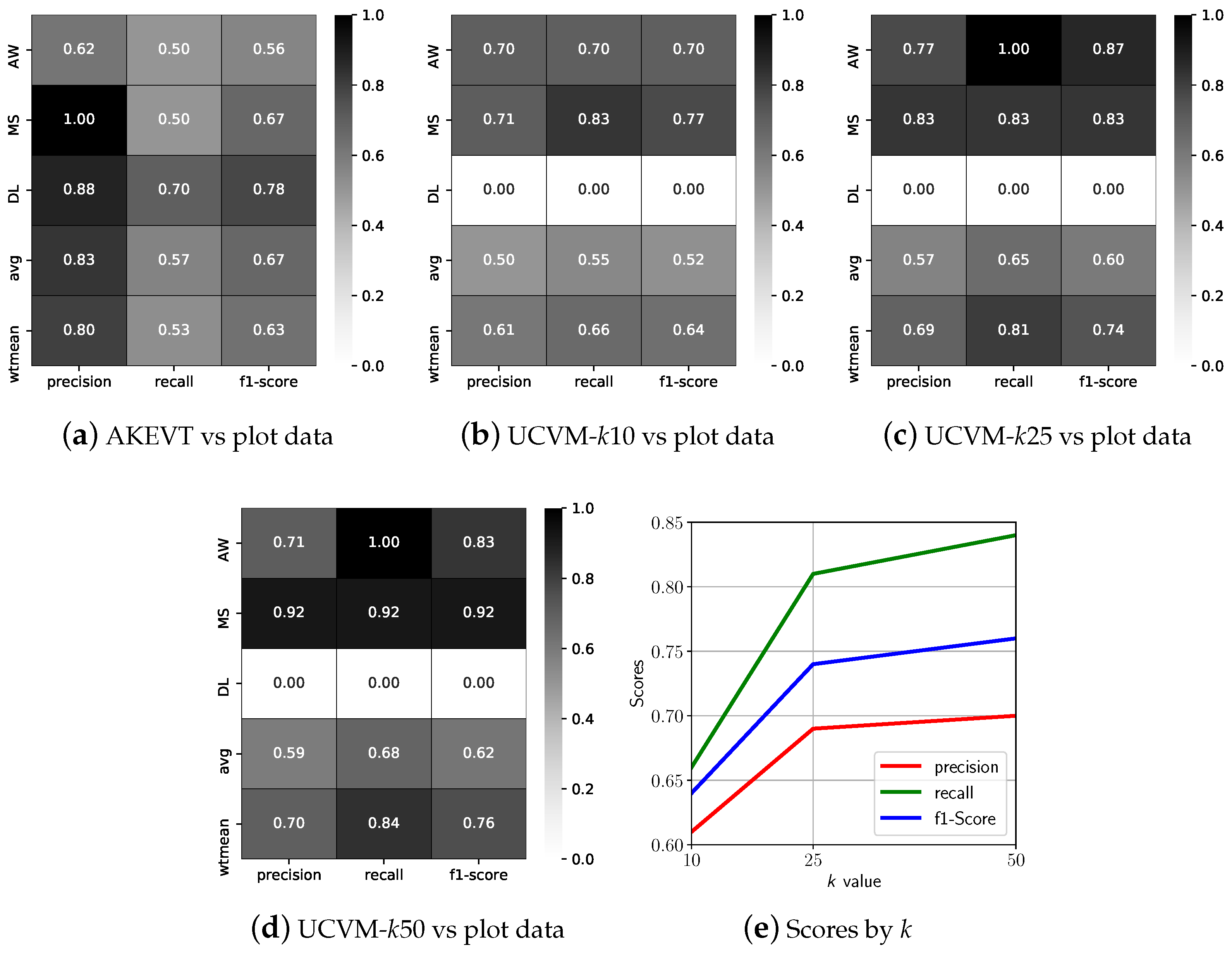
The AKEVT vegetation map is used as key training dataset for development of high resolution vegetation map in our study. To establish the baseline accuracy of our training dataset we evaluated it against observations collected at 30 field plots. Field based validation were limited to Alder-Willow Shrub, Mixed Shrub-Sedge Tussock Tundra-Bog and Dryas/Lichen Dwarf Shrub Tundra classes for which observations were available. Figure 6a shows the precision, recall, and F1-score of the AKEVT map and the 30 field plots. The average precision, recall, and F1-score were 0.83, 0.57, and 0.67, respectively. The weighted mean, which weights the average scores by land cover area Table 1, scores were 0.80, 0.53, and 0.63 for precision, recall, and F1-score, respectively. Dryas/Lichen Dwarf Shrub Tundra showed the best scores, while Alder-Willow Shrub performed the worst for the AKEVT map. Mixed Shrub-Sedge Tussock Tundra-Bog had high precision but low recall scores indicating potential misclassification in the AKEVT map.
Figure 6b–d shows the best scoring cases when unsupervised clustering were performed at k = 10, 25 and 50 levels of division. Similar to the study region, unsupervised clustering at higher levels of division (k = 25, and 50) led to better scores than at fewer clusters (k = 10). Alder-Willow Shrub and Mixed Shrub-Sedge Tussock Tundra-Bog for k = 50 had the overall best scores. The cluster k = 25 had higher scores of 0.69, 0.81, and 0.74 for precision, recall, and F1-score, respectively. The cluster k = 50 performed slightly better, with average scores of 0.70, 0.84, and 0.76 for precision, recall, and F1-score, respectively. Field observation based validation of UCVM shows improved accuracy of the vegetation map over AKEVT (Figure 6a). Unsupervised classification algorithm ensures grouping of pixels with similar vegetation and thus similar spectral response together, and eliminates misclassifications and noise within AKEVT map.
However, none of the UCVM maps were able to correctly map any of the 10 Dryas/Lichen Dwarf Shrub Tundra vegetation plots. Poor classification of Dryas/Lichen Dwarf Shrub Tundra indicates lack of consistent patterns in remote sensing dataset across the class in AKEVT map. This could be due to a number of reasons, potentially due to the low area amount over the study region (Table 1) and how the UCVM method is performed (i.e., taking the most dominant vegetation type in the cluster).
UCVM maps produced with unsupervised classification at k = 50 level of division showed overall best accuracy and consistent validation statistics for both validation datasets for all vegetation classes. Thus, k = 50 based UCVM was selected as training dataset for developing CNN models in our study. Here on we refer to k = 50 based UCVM map as UCVM map. Table 3 shows the area distribution of all vegetation classes within UCVM map, which show slight differences in distribution of classes than the AKEVT map (Table 1), especially for the Dryas/Lichen Dwarf Shrub Tundra class.
4.2. Analysis of Datasets
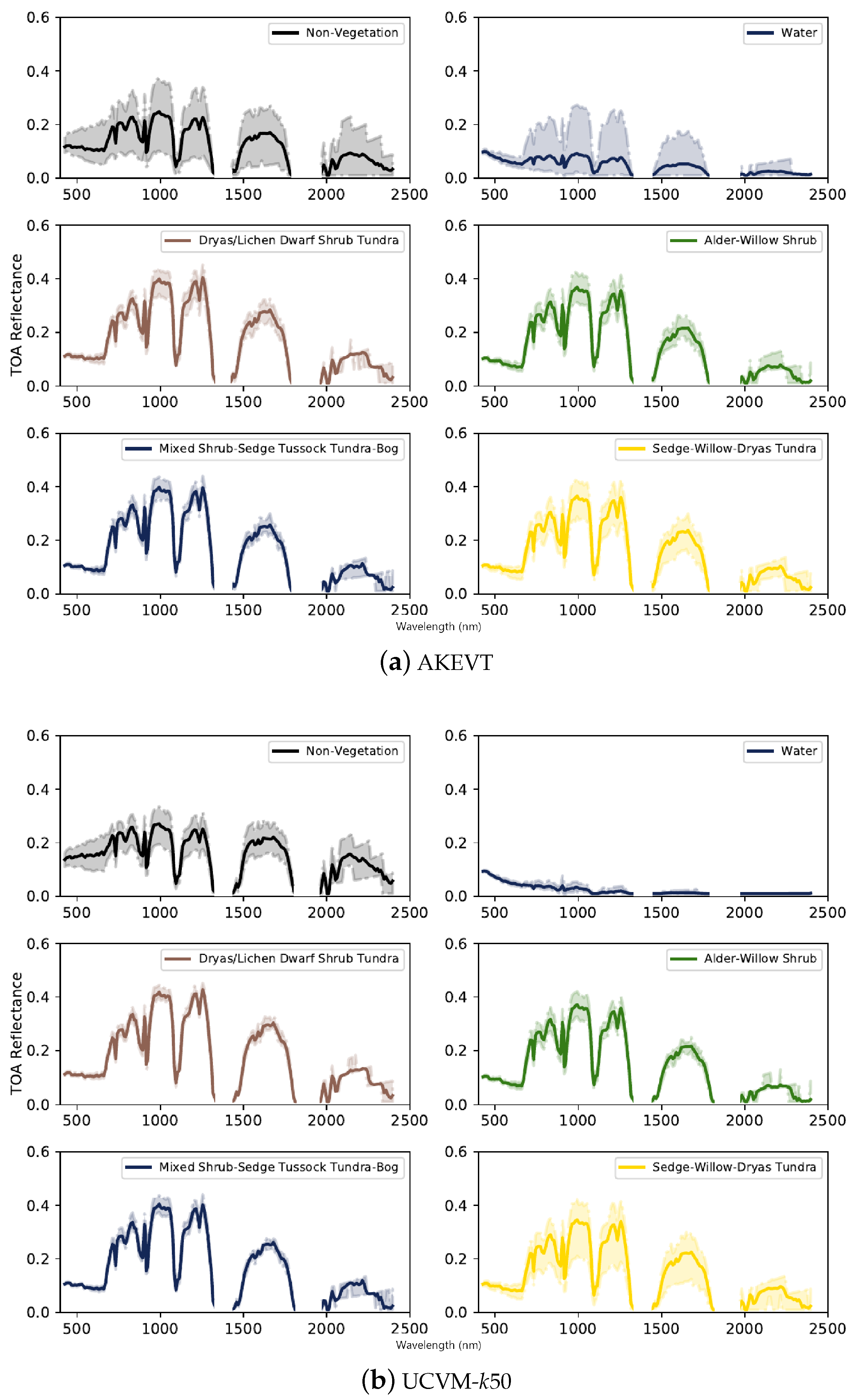
After the re-sampling of datasets to 5 m (Figure 2), all datasets were analyzed to understand the best attributes across the vegetation classes in the AKEVT map. We analyzed the patterns and distributions of each dataset in order to get a better understanding of the similarities and differences among their values for each vegetation class. Figure 7 shows the spectral response for EO-1 Hyperion within each vegetation class within UCVM and AKEVT datasets. Compared to AKEVT (Figure 7b, spectral response within UCVM vegetation classes demonstrate significant less variability.
For both datasets, similar trends were found. The Sedge-Willow-Dryas Tundra and Alder-Willow Shrub class had similar reflectance values for the majority of the bands with separation around 1500–1800 nm. There was a similar trend for the Mixed Shrub-Sedge Tussock Tundra-Bog and Dryas/Lichen Dwarf Shrub Tundra with separation around 1500–1800 nm. The water and non-vegetated classes had lower reflectance values through most bands (600–2500 nm) compared to the other classes.
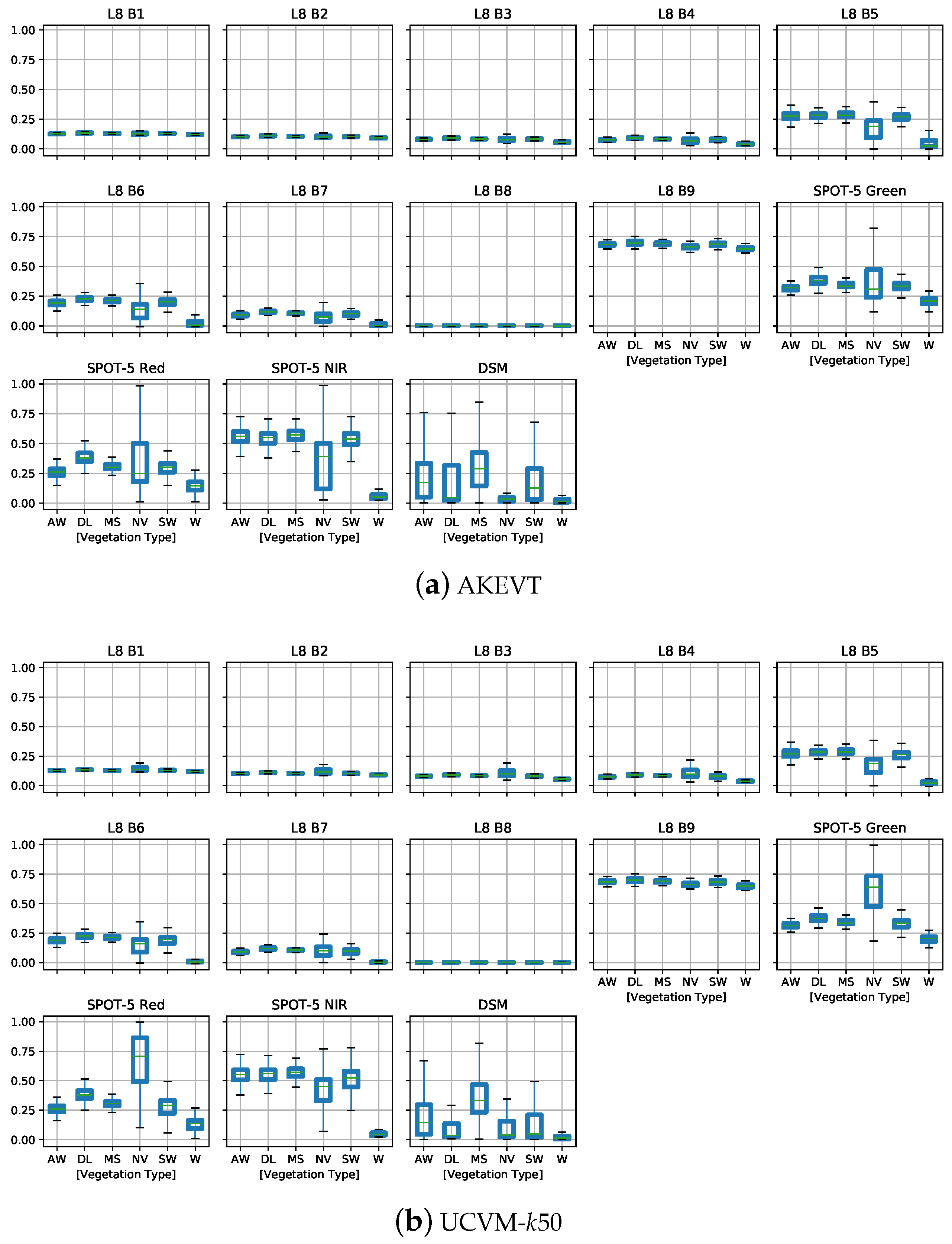
Figure 8 presents the distribution of the SPOT-5, DSM, and Landsat 8 data for the vegetation classes over the study region for the AKEVT and UCVM datasets. The box-plot shows some sensors/bands may be better suited than the others for classifying certain vegetation types. The non-vegetated class shows the greatest range between the minimum and maximum values, indicating potential lumping of different vegetation types and thus potential sources of error in the AKEVT map. All of the classes with vegetation show little differences in values for most datasets.
Landsat 8 bands 5, 6, and 7, representing the near infrared (NIR) and shortwave infrared parts of the spectrum, provided the best distinction between vegetation classes among all Landsat bands. Most of the vegetation classes showed sensitivity in the multispectral green, red, and NIR bands of SPOT-5; however, they also showed a large range of variability in their responses (Figure 8). The DSM topographic properties of the vegetation classes had distinguishable differences. However, similar to SPOT-5, DSM showed a large range of variability.
4.3. CNN Based Vegetation Maps
4.3.1. Training CNN Models
Due to limited number of observations from field plots, they were insufficient to be used for training models, and thus were used only for validation of vegetation products. Field based validation were limited to Alder-Willow Shrub, Mixed Shrub-Sedge Tussock Tundra-Bog and Dryas/Lichen Dwarf Shrub Tundra classes for which observations were available. CNN models were trained using AKEVT and UCVM labels, for patch sizes of 3 × 3, 6 × 6, and 12 × 12. Figure 9 shows the convergence behavior of CNN models when trained using the two training datasets for 100 epochs. While the 3 × 3 patch size CNN-AKEVT models (Figure 9a–c) converged with ∼68% accuracy, the 3 × 3 patch size CNN-UCVM models (Figure 9d–f) achieved ∼97% accuracy. The lower training scores using the AKEVT can be attributed to the noise within the dataset. The 6 × 6 and 12 × 12 CNN-AKEVT models tend to overfit after 60 and 30 epochs, respectively. Additionally, the 12 × 12 CNN-UCVM models tend to overfit after 60 epochs, indicating that smaller patch sizes might be favorable for our study. The 3 × 3 patch size for both models show no overfitting and also lead to better validation scores using the randomly sampled test datasets. It should be noted that the CNN architecture and hyperparameters do not change for the CNN-UCVM and CNN-AKEVT models and the performance is solely based on the randomly sample extracted data from the UCVM and AKEVT vegetation products.
4.3.2. CNN Models Trained Using UCVM
CNN models trained using UCVM were developed using 3 × 3, 6 × 6, and 12 × 12 patches. Vegetation maps developed were validated against the field vegetation observation (Figure 10). All CNN-UCVM models performed well for the Alder-Willow Shrub and Mixed Shrub-Sedge Tussock Tundra-Bog classes, however, were unable to classify the Dryas/Lichen Dwarf Shrub Tundra class. The 6 × 6 patch based CNN-UCVM performed the best with weighted mean precision, recall and F1 scores of 0.67, 0.83, and 0.74, respectively. The 12 × 12 patch based CNN-UCVM had the lowest validation scores, with weighted precision, recall and F1 scores of 0.62, 0.63, and 0.62, respectively. The 3 × 3 patch based CNN-UCVM had slightly lower scores than 6 × 6 patch, with weighted precision, recall and F1 scores of 0.69, 0.79, and 0.73, respectively. The 6 × 6 patch based CNN-UCVM validation metrics were similar to using UCVM alone (Figure 6) but significant improvement (F1 score from 0.63 to 0.74) over the original AKEVT map (Figure 6). This was primarily driven by the high validation scores for the Alder-Willow Shrubs and Mixed Shrub-Sedge Tussock Tundra-Bog classes that were the dominant vegetation within the Kougarok watershed.
4.3.3. CNN Models Trained with AKEVT
Figure 11 shows the validation statistics against the field vegetation observations using 3 × 3, 6 × 6, and 12 × 12 patches for the CNN model based on the AKEVT dataset (CNN-AKEVT). All CNN-AKEVT models performed best for the Alder-Willow Shrub class. The 3 × 3 patch based CNN-AKEVT performed the best with weighted precision, recall and F1 scores of 0.73, 0.75, and 0.73, respectively. The 3 × 3 patch based CNN-AKEVT had similar scores for the Dryas/Lichen Dwarf Shrub Tundra and Mixed Shrub-Sedge Tussock Tundra-Bog classes. The 12 × 12 patch based CNN-AKEVT had the lowest validation scores, with weighted precision, recall and F1 scores of 0.64, 0.64, and 0.65, respectively. The 6 × 6 patch based CNN-AKEVT had slighter higher validation scores than using 12 × 12 patches, with weighted precision, recall and F1 scores of 0.80, 0.69, and 0.73, respectively.
4.3.4. Summary of Best Performing Models
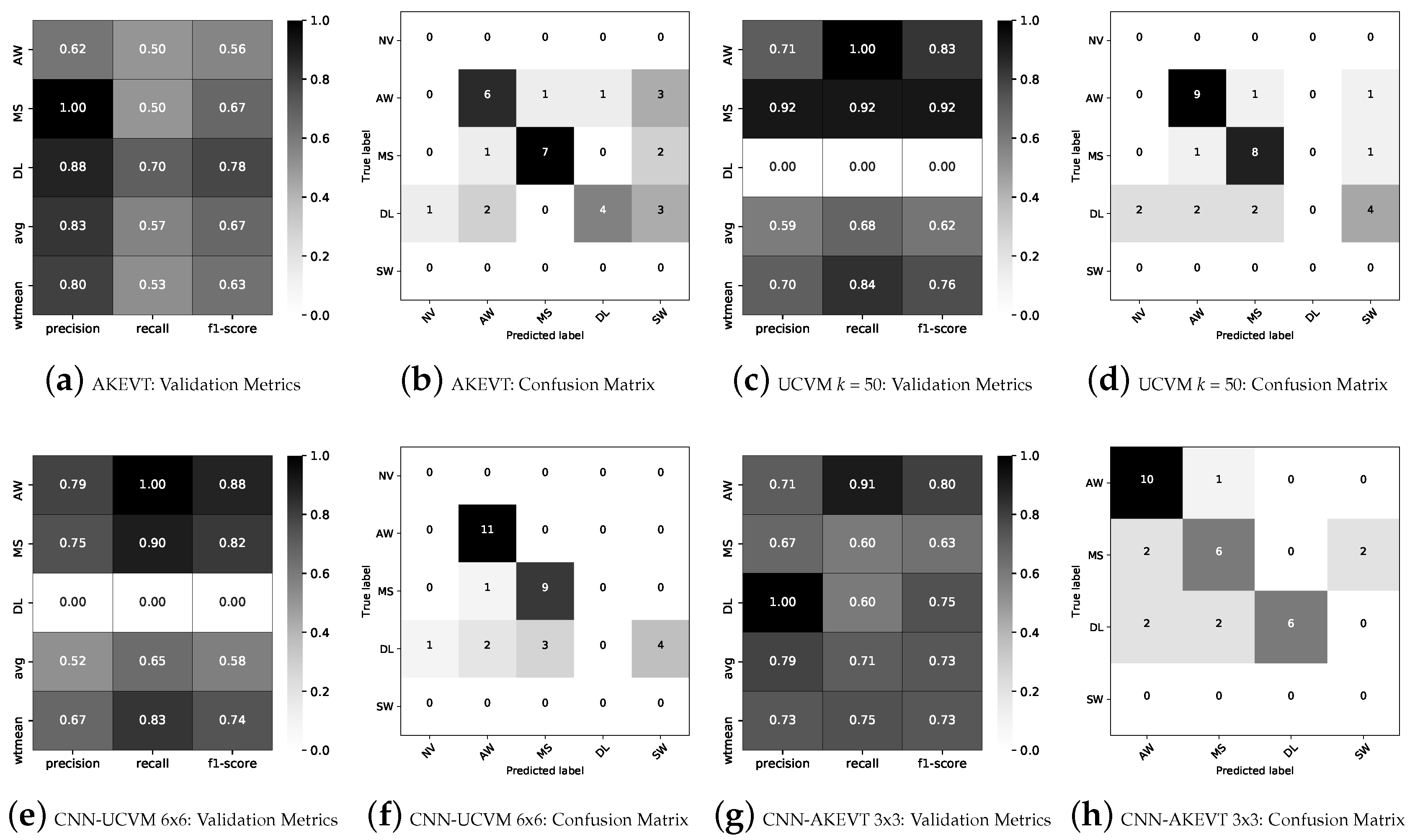
Figure 12 shows the 6 × 6 CNN-UCVM map, which performed best against the field plots over all other models and approaches. This CNN-UCVM vegetation map is available at http://dx.doi.org/10.5440/1418854 (Supplementary Materials). Figure 13 shows the summary of validation metrics for the vegetation maps developed and analyzed in this study. Confusion matrices for each model (Figure 13) show the frequencies of false classifications by vegetation type. The Dryas/Lichen Dwarf Shrub Tundra class was often misclassified by all CNN models as Sedge-Willow-Dryas Tundra.
The AKEVT dataset showed the worst misclassification, with 18 instances spread equally across most classes. UCVM at k = 50 had 14 instances of misclassification, with the majority in the Dryas/Lichen Dwarf Shrub Tundra class. The CNN-UCVM using 6 × 6 patch size had 11 instances of misclassification, with the majority in the Dryas/Lichen Dwarf Shrub Tundra class and only one misclassification outside this class. The CNN-AKEVT using 3 × 3 patch size had 9 instances of misclassification, with Dryas/Lichen Dwarf Shrub Tundra class and Mixed Shrub-Sedge Tussock Tundra-Bog class performing the worst.
5. Discussion
5.1. Vegetation Classification Trends
Comparison with field-based observations indicated that the CNN models trained with both the AKEVT and UCVM maps achieved high accuracies for the Alder-Willow Shrub and the Mixed Shrub-Sedge Tussock Tundra-Bog classes, but the models could not robustly distinguish the Dryas/Lichen Dwarf Shrub Tundra class. However, this class exhibited identifiable spectral characteristics, especially in the EO-1 dataset, compared to other vegetation classes (Figure 7). The low validation scores for Dryas/Lichen Dwarf Shrub Tundra were most likely due to the small area presence in the region and thus a low number of training samples (Table 1).
Alder-Willow Shrubs and Mixed Shrub-Sedge Tussock Tundra-Bog were mapped with sufficient accuracy by all the CNN models. Both were dominant vegetation classes in the region and were thus well-represented in the training dataset (Table 3) used to develop the CNN models. Additionally, these vegetation types exhibited distinguishing spectral characteristics, especially in the EO-1, SPOT-5, Landsat 8 OLI and DSM datasets (Figure 7 and Figure 8). The confusion matrices (Figure 13) helped identify needed observations that could enhance the training dataset so the models could better distinguish frequently misclassified vegetation types, like Dryas/Lichen Dwarf Shrub Tundra and Sedge-Willow-Dryas Tundra.
While this study was focused at the Seward Peninsula, where the NGEE Arctic project is conducting extensive ground measurements, the analysis could be extended to the entire State of Alaska since many of the datasets used here are available state wide. The CNN-derived vegetation maps we developed showed improved accuracy in mapping vegetation classes compared to the AKEVT map itself, which was used to train the models. Comparisons with field observations suggested that datasets developed for large extents using sparse validation data can lead to low validation scores (Figure 6), probably due to training data limitations. Information rich high-resolution remote sensing data underlying the quantitative methods demonstrated here help ensure consistency across and within vegetation classes for small study regions, such as the Kougarok Watershed.
5.2. Remote Sensing Datasets & Multisensor Fusion
High-resolution (∼0.3–10 m) satellite imagery (e.g., IKONOS, QuickBird, SPOT-5, and WorldView) are becoming increasingly available for Arctic and boreal ecosystems. These data products offer opportunities to evaluate and improve upon existing vegetation and land cover maps for high latitude regions, such as AKEVT, and at continental scales, like the National Land Cover Database (NLCD) maps. One of the main goals of this study was to develop high-resolution vegetation datasets for the Seward Peninsula of Alaska to aid ecological research and modeling studies in the region. This study was a first step toward development of a machine learning framework to fuse high-resolution datasets from a range of remote sensing products to develop an accurate and high-resolution geospatial mapping of vegetation and land cover for high latitude ecosystems.
We have shown that EO-1, SPOT-5, Landsat 8 OLI, and IfSAR datasets can be used to distinguish different classes of vegetation in high latitude ecosystems. The EO-1 hyperspectral dataset was particularly valuable for distinguishing between the primary vegetation classes (Figure 7), while SPOT-5 provided a high spatial resolution, commensurate with the scales at which field vegetation studies are conducted. Future work includes collecting high-resolution imagery from a variety of sensing modalities (e.g., optical, SAR).
Freely available datasets were chosen for this study, but other high-resolution commercial satellite products (e.g., from WorldView-2, 3 [12,45]) may also be well suited for improving accuracy and resolution of vegetation maps. The remote sensing data used here represents, like in most remote sensing studies, a snapshot in time of current land surface conditions. A large database of freely available optical and SAR images are available that could be used for characterizing vegetation dynamics across the State of Alaska. Recent greening and increases in shrub cover are important dynamics of interest in terrestrial Arctic research, associated with increases in local evapotranspiration, soil active layer depth, and permafrost degradation [46]. Using spatio-temporal time series of high spectral and spatial resolution datasets, methods developed in this study can be applied to map and characterize vegetation dynamics in high latitude regions. Additionally, future research includes collecting imagery over the same period as current field surveys for accurate validation data products that can be used for assessing dynamic vegetation models.
5.3. Training Label Generation
Vegetation maps developed using the UCVM and CNN approaches both demonstrated good accuracy during the validation process. The low precision, recall, and F1-score for the Dryas/Lichen Dwarf Shrub Tundra class for the UCVM (Figure 6) and CNN-UCVM (Figure 10) methods could be due to limited training samples for this rare vegetation type in the watershed. Additionally, this is compounded by how the UCVM method is performed by taking the most dominant vegetation type in the cluster. Increasing the cluster size (e.g., k = 1000) may help distinguish the Dryas/Lichen Dwarf Shrub Tundra class and will be evaluated in future studies. Also, splitting the datasets at other increments (i.e., instead of 90% for training) could provide more insights. However, initial tests showed minor variations of validation scores and showed similar trends when updating the training data using the UCVM method.
The unsupervised classification step in the UCVM method creates classes that are spectrally similar and may thus remove some of the noise and confounding effects. As a result, CNN models trained with UCVM lead to better accuracy compared to those trained with only the AKEVT in the study region (Figure 9). Compared to AKEVT, the UCVM map provides a higher resolution distribution of vegetation classes (Figure 5). Mapcurves-based labeling of the clustering-based map from UCVM employed a nearest-neighbor re-sampling method; however, more sophisticated re-sampling methods may lead to improved labeling accuracy. GOF maps from Mapcurves (Figure 5d,h) show the spatial uncertainty in classification accuracy within the UCVM map. While Alder-Willow Shrub and Mixed Shrub-Sedge Tussock Tundra-Bog often had a higher GOF, and thus lower uncertainty, Dryas/Lichen Dwarf Shrub Tundra and Sedge-Willow-Dryas Tundra had low GOFs and thus higher uncertainty in the UCVM map.
High quality training data are critically important for training machine learning methods like CNNs. Additional field observations are needed to determine if producing training labels by this method can further enhance vegetation classifications. GOF maps provide insights into the vegetation types and locations that require additional measurements to enhance the training dataset.
Another possible approach for creating training datasets is the use of generative adversarial networks (GANs), which is an approach that maps a random vector to an image such that the generated image is indistinguishable from the real one [47]. For Arctic vegetation mapping, GANs would be created for each vegetation class that matches spectral and spatial characteristics. Furthermore, several modifications to the standard GAN algorithm could be performed to achieve optimal results without labeled real data [48]. Also, augmentation methods (e.g., zooming, flipping, whitening) could be used to increase the data size but was out of scope for this study and will need to be looked into for future studies.
5.4. CNN Model Architecture
Overall, the CNN based models performed better for field-scale mapping compared to the UCVM method and the AKEVT map. The patch size used for developing the CNN models played an important role in the classification. Each image patch was input to the model independently, which means that only the “intra-patch” context information was considered [49] when building the CNN models. The correlations between patches were not taken into account, which might lead to gaps between patches [49]. However, this may only apply to objects with strong continuity, such as urban features, which were not present in the imagery. Use of correct patch sizes that can differentiate vegetation classes on the landscape would lead to improved classifications, and thus we explored a range of sizes to identify the best patch size parameters. Smaller patch sizes (3 × 3 and 6 × 6) performed better for both CNN models.
Despite the noise in the AKEVT dataset, CNNs were able to learn meaningful representations that helped to associate vegetation classes with the satellite datasets. A more sophisticated analysis could be performed to characterize spatial patterns of uncertainty within the AKEVT dataset. For example, a dropout regularization could be added to the weights of the noise during training [50]. Additionally, novel loss functions could be implemented for capturing classification errors from both the majority and minority classes equally [51].
In future studies, the exploration of CNN architectures that leverage high-spectral resolutions could result in better mappings at the field scale. For example, a CNN with two branches that leverage high spectral and spatial resolutions could lead to better accuracies [52]. Employing other activation functions, such as exponential linear units (ELUs), could provide further performance improvements [53]. Additionally, further exploration of hyperparameters (e.g., learning rate, loss function, weight initialization) could help optimize the CNN approach.
6. Conclusions
Accurate vegetation maps are important for understanding terrestrial biosphere processes in high latitude ecosystems. Given the importance of vegetation dynamics in Alaska and the associated impacts of climate change, there is a need for up-to-date and high-resolution vegetation maps. The use of high spectral and spatial remote sensing products were evaluated for vegetation mapping in the southern Seward Peninsula, Alaska, at 5 m resolution. A multisensor data fusion approach was developed to exploit data available from a variety of different remote sensing platforms at a range of spatial resolutions to characterize and map vegetation in Arctic ecosystem. An unsupervised technique was developed to classify the remote sensing datasets into clusters and employed a quantitative method to add supervision to the unlabeled clusters, producing a fully labeled vegetation map. Two CNN models were developed from the original map and the re-labeled map. Vegetation measurements were collected across key vegetation types at the field sites in the Kougarok Watershed, and the vegetation products were validated against these observations. Vegetation maps developed in the study demonstrated high accuracy through the validation exercises. Our analysis demonstrated that CNN models are capable of accurately mapping vegetation based on multisensor remote sensing imagery. Specifically, the CNN model based on the labels using the unsupervised technique outperformed the CNN based on the AKEVT labels. Additionally, the CNN model based on the UCVM dataset increased the recall score from the original AKEVT dataset from 0.53 to 0.83.
The EO-1, SPOT-5, Landsat 8 OLI, and IfSAR datasets were found to provide the best predictive ability in the CNN models, specifically for Alder-Willow Shrub and Mixed Shrub-Sedge Tussock Tundra-Bog. High spectral resolution datasets were demonstrated to provide distinguishing characteristics among vegetation communities in the Seward Peninsula study area. Thus, the fusion of high spatial and spectral resolution datasets are useful for mapping vegetation at the field-to-regional scale in high latitude ecosystems. We produced one of the most accurate, high resolution, field-validated vegetation maps for the Seward Peninsula of Alaska. Characterizing the distribution of vegetation in the tundra is critically important to understanding the ecological processes in these ecosystems, which are undergoing changes due to climate change. We developed a machine learning framework to exploit data from a range of remote sensing platforms becoming available in the region to improve the understanding the shifting patterns and distribution of diverse Arctic and boreal vegetation.
Supplementary Materials
The CNN vegetation map [54] is available at http://dx.doi.org/10.5440/1418854.
Author Contributions
Z.L.L. led the study. Z.L.L., J.K. and F.M.H. formulated and developed the research methodology for this study. Z.L.L. performed the processing of the remote sensing imagery and development of the CNN models. J.K. and F.M.H. developed the clustering algorithm. A.L.B. and C.M.I. collected the field vegetation observations. All authors contributed to the writing of the manuscript.
Funding
The Next-Generation Ecosystem Experiments (NGEE Arctic) project is supported by the US Department of Energy, Office of Science, Biological and Environmental Research Program.
Acknowledgments
The Next-Generation Ecosystem Experiments (NGEE Arctic) project is supported by the Office of Biological and Environmental Research in the DOE Office of Science. This manuscript has been authored by UT-Battelle, LLC under Contract No. DE-AC05-00OR22725 with the U.S. Department of Energy. The United States Government retains and the publisher, by accepting the article for publication, acknowledges that the United States Government retains a non-exclusive, paid-up, irrevocable, world-wide license to publish or reproduce the published form of this manuscript, or allow others to do so, for United States Government purposes. The Department of Energy will provide public access to these results of federally sponsored research in accordance with the DOE Public Access Plan (http://energy.gov/downloads/doe-public-access-plan).
Conflicts of Interest
The authors declare no conflict of interest.
References
- Overland, J.E.; Wang, M.; Walsh, J.E.; Stroeve, J.C. Future Arctic climate changes: Adaptation and mitigation time scales. Earth’s Future 2014, 2, 68–74. [Google Scholar] [CrossRef] [Green Version]
- Lader, R.; Walsh, J.E.; Bhatt, U.S.; Bieniek, P.A. Projections of Twenty-First-Century Climate Extremes for Alaska via Dynamical Downscaling and Quantile Mapping. J. Appl. Meteorol. Climatol. 2017, 56, 2393–2409. [Google Scholar] [CrossRef]
- Zhang, W.; Miller, P.A.; Smith, B.; Wania, R.; Koenigk, T.; Döscher, R. Tundra shrubification and tree-line advance amplify arctic climate warming: results from an individual-based dynamic vegetation model. Environ. Res. Lett. 2013, 8, 034023. [Google Scholar] [CrossRef] [Green Version]
- Tranvik, L. Carbon cycling in the Arctic. Science 2014, 345, 870. [Google Scholar] [CrossRef] [PubMed]
- Pearson, R.G.; Phillips, S.J.; Loranty, M.M.; Beck, P.S.A.; Damoulas, T.; Knight, S.J.; Goetz, S.J. Shifts in Arctic vegetation and associated feedbacks under climate change. Nat. Clim. Chang. 2013, 3, 673–677. [Google Scholar] [CrossRef] [Green Version]
- Lawrence, D.M.; Swenson, S.C. Permafrost response to increasing Arctic shrub abundance depends on the relative influence of shrubs on local soil cooling versus large-scale climate warming. Environ. Res. Lett. 2011, 6, 045504. [Google Scholar] [CrossRef] [Green Version]
- McGuire, A.D.; Koven, C.; Lawrence, D.M.; Clein, J.S.; Xia, J.; Beer, C.; Burke, E.; Chen, G.; Chen, X.; Delire, C.; et al. Variability in the sensitivity among model simulations of permafrost and carbon dynamics in the permafrost region between 1960 and 2009. Glob. Biogeochem. Cycles 2016, 30, 1015–1037. [Google Scholar] [CrossRef] [Green Version]
- Rupp, T.S.; Chapin, F.S.; Starfield, A.M. Response of subarctic vegetation to transient climatic change on the Seward Peninsula in north-west Alaska. Glob. Chang. Biol. 2000, 6, 541–555. [Google Scholar] [CrossRef] [Green Version]
- Higuera, P.; Peters, M.; Brubaker, L.; Gavin, D. Frequent Fires in Ancient Shrub Tundra: Implications of Paleorecords for Arctic Environmental Change. PLoS ONE 2008, 3, e0001744. [Google Scholar] [CrossRef]
- Tang, G.; Yuan, F.; Bisht, G.; Hammond, G.E.; Lichtner, P.C.; Kumar, J.; Mills, R.T.; Xu, X.; Andre, B.; Hoffman, F.M.; et al. Addressing Numerical Challenges in Introducing a Reactive Transport Code into a Land Surface Model: A Biogeochemical Modeling Proof-of-concept with CLM–PFLOTRAN 1.0. Geosci. Model Dev. 2016, 9, 927–946. [Google Scholar] [CrossRef]
- Bisht, G.; Huang, M.; Zhou, T.; Chen, X.; Dai, H.; Hammond, G.; Riley, W.; Downs, J.; Liu, Y.; Zachara, J. Coupling a three-dimensional subsurface flow and transport model with a land surface model to simulate stream-aquifer-land interactions (PFLOTRAN_CLM v1.0). Geosci. Model Dev. Discuss. 2017, 10, 4539–4562. [Google Scholar] [CrossRef]
- Langford, Z.; Kumar, J.; Hoffman, F.M.; Norby, R.J.; Wullschleger, S.D.; Sloan, V.L.; Iversen, C.M. Mapping Arctic Plant Functional Type Distributions in the Barrow Environmental Observatory Using WorldView-2 and LiDAR Datasets. Remote Sens. 2016, 8, 733. [Google Scholar] [CrossRef]
- Lindsay, C.; Zhu, J.; Miller, A.E.; Kirchner, P.; Wilson, T.L. Deriving Snow Cover Metrics for Alaska from MODIS. Remote Sens. 2015, 7, 12961–12985. [Google Scholar] [CrossRef] [Green Version]
- Macander, M.J.; Frost, G.V.; Nelson, P.R.; Swingley, C.S. Regional Quantitative Cover Mapping of Tundra Plant Functional Types in Arctic Alaska. Remote Sens. 2017, 9, 1024. [Google Scholar] [CrossRef]
- Verbyla, D.; Hegel, T.; Nolin, A.W.; van de Kerk, M.; Kurkowski, T.A.; Prugh, L.R. Remote Sensing of 2000–2016 Alpine Spring Snowline Elevation in Dall Sheep Mountain Ranges of Alaska and Western Canada. Remote Sens. 2017, 9, 1157. [Google Scholar] [CrossRef]
- Bratsch, S.N.; Epstein, H.E.; Buchhorn, M.; Walker, D.A. Differentiating among Four Arctic Tundra Plant Communities at Ivotuk, Alaska Using Field Spectroscopy. Remote Sens. 2016, 8, 51. [Google Scholar] [CrossRef]
- Davidson, S.J.; Santos, M.J.; Sloan, V.L.; Watts, J.D.; Phoenix, G.K.; Oechel, W.C.; Zona, D. Mapping Arctic Tundra Vegetation Communities Using Field Spectroscopy and Multispectral Satellite Data in North Alaska, USA. Remote Sens. 2016, 8, 978. [Google Scholar] [CrossRef]
- Schmitt, M.; Zhu, X.X. Data Fusion and Remote Sensing: An ever-growing relationship. IEEE Geosci. Remote Sens. Mag. 2016, 4, 6–23. [Google Scholar] [CrossRef]
- Chen, Y.; Li, C.; Ghamisi, P.; Jia, X.; Gu, Y. Deep Fusion of Remote Sensing Data for Accurate Classification. IEEE Geosci. Remote Sens. Lett. 2017, 14, 1253–1257. [Google Scholar] [CrossRef]
- Hargrove, W.W.; Hoffman, F.M.; Hessburg, P.F. Mapcurves: A Quantitative Method for Comparing Categorical Maps. J. Geogr. Syst. 2006, 8, 187–208. [Google Scholar] [CrossRef]
- Bond-Lamberty, B.; Epron, D.; Harden, J.; Harmon, M.E.; Hoffman, F.M.; Kumar, J.; McGuire, A.D.; Vargas, R. Estimating Heterotrophic Respiration at Large Scales: Challenges, Approaches, and Next Steps. Ecosphere 2016, 7, e01380. [Google Scholar] [CrossRef]
- Lecun, Y.; Bengio, Y.; Hinton, G. Deep learning. Nature 2015, 521, 436–444. [Google Scholar] [CrossRef] [PubMed]
- Zhang, L.; Zhang, L.; Du, B. Deep Learning for Remote Sensing Data: A Technical Tutorial on the State of the Art. IEEE Geosci. Remote Sens. Mag. 2016, 4, 22–40. [Google Scholar] [CrossRef]
- Langford, Z.L.; Kumar, J.; Hoffman, F.M. Convolutional Neural Network Approach for Mapping Arctic Vegetation using Multi-Sensor Remote Sensing Fusion. In Proceedings of the 2017 IEEE International Conference on Data Mining Workshops (ICDMW 2017), New Orleans, LA, USA, 18–21 November 2017; Institute of Electrical and Electronics Engineers (IEEE): Piscataway, NJ, USA; Conference Publishing Services (CPS): Washington, DC, USA, 2017. [Google Scholar] [CrossRef]
- Xie, W.; Li, Y. Hyperspectral Imagery Denoising by Deep Learning With Trainable Nonlinearity Function. IEEE Geosci. Remote Sens. Lett. 2017, 14, 1963–1967. [Google Scholar] [CrossRef]
- Xu, X.; Li, W.; Ran, Q.; Du, Q.; Gao, L.; Zhang, B. Multisource Remote Sensing Data Classification Based on Convolutional Neural Network. IEEE Trans. Geosci. Remote Sens. 2018, 56, 937–949. [Google Scholar] [CrossRef]
- Hunt, S.; Yu, Z.; Jones, M. Lateglacial and Holocene climate, disturbance and permafrost peatland dynamics on the Seward Peninsula, western Alaska. Quat. Sci. Rev. 2013, 63, 42–58. [Google Scholar] [CrossRef]
- Silapaswan, C.; Verbyla, D.; McGuire, A. Land Cover Change on the Seward Peninsula: The Use of Remote Sensing to Evaluate the Potential Influences of Climate Warming on Historical Vegetation Dynamics. Can. J. Remote Sens. 2001, 27, 542–554. [Google Scholar] [CrossRef]
- Viereck, L.A. The Alaska Vegetation Classification; General technical report; USDA Pacific Northwest Research Station: Corvallis, OR, USA, 1992.
- Narita, K.; Harada, K.; Saito, K.; Sawada, Y.; Fukuda, M.; Tsuyuzaki, S. Vegetation and Permafrost Thaw Depth 10 Years after a Tundra Fire in 2002, Seward Peninsula, Alaska. Arct. Antarct. Alp. Res. 2015, 47, 547–559. [Google Scholar] [CrossRef] [Green Version]
- Hinzman, L.D.; Kane, D.L.; Yoshikawa, K.; Carr, A.; Bolton, W.R.; Fraver, M. Hydrological variations among watersheds with varying degrees of permafrost. In Proceedings of the 8th International Conference on Permafrost, Zurich, Switzerland, 21–25 July 2003; A.A. Balkema: Exton, PA, USA, 2003; pp. 407–411. [Google Scholar]
- Walker, D.A.; Breen, A.L.; Druckenmiller, L.A.; Wirth, L.W.; Fisher, W.; Raynolds, M.K.; Sibík, J.; Walker, M.D.; Hennekens, S.; Boggs, K.; et al. The Alaska Arctic Vegetation Archive (AVA-AK). Phytocoenologia 2016, 46, 221–229. [Google Scholar] [CrossRef] [Green Version]
- Raynolds, M.K.; Walker, D.A.; Maier, H.A. Plant community-level mapping of arctic Alaska based on the Circumpolar Arctic Vegetation Map. Phytocoenologia 2005, 35, 821–848. [Google Scholar] [CrossRef]
- Hartigan, J.A. Clustering Algorithms; John Wiley & Sons: Hoboken, NJ, USA, 1975; p. 351. [Google Scholar]
- Hoffman, F.M.; Hargrove, W.W.; Mills, R.T.; Mahajan, S.; Erickson, D.J.; Oglesby, R.J. Multivariate Spatio-Temporal Clustering (MSTC) as a Data Mining Tool for Environmental Applications. In Proceedings of the iEMSs Fourth Biennial Meeting: International Congress on Environmental Modelling and Software Society (iEMSs 2008), Barcelona, Spain, 7–10 July 2008; pp. 1774–1781. [Google Scholar]
- Bradley, P.S.; Fayyad, U.M. Refining Initial Points for K-Means Clustering. In Proceedings of the Fifteenth International Conference on Machine Learning, Madison, WI, USA, 24–27 July 1998; Morgan Kaufmann Publishers Inc.: San Francisco, CA, USA, 1998; pp. 91–99. [Google Scholar]
- Kumar, J.; Mills, R.T.; Hoffman, F.M.; Hargrove, W.W. Parallel k-Means Clustering for Quantitative Ecoregion Delineation Using Large Data Sets. In Proceedings of the International Conference on Computational Science (ICCS 2011), Singapore, 1–3 June 2011; Sato, M., Matsuoka, S., Sloot, P.M., van Albada, G.D., Dongarra, J., Eds.; Elsevier: Amsterdam, The Netherlands, 2011; Volume 4, pp. 1602–1611. [Google Scholar] [CrossRef]
- Halko, N.; Martinsson, P.G.; Tropp, J.A. Finding structure with randomness: Probabilistic algorithms for constructing approximate matrix decompositions. arXiv, 2009; arXiv:math.NA/0909.4061. [Google Scholar] [CrossRef]
- Krizhevsky, A.; Sutskever, I.; Hinton, G.E. ImageNet Classification with Deep Convolutional Neural Networks. In Advances in Neural Information Processing Systems 25; Pereira, F., Burges, C.J.C., Bottou, L., Weinberger, K.Q., Eds.; Curran Associates, Inc.: Red Hook, NY, USA, 2012; pp. 1097–1105. [Google Scholar]
- Zeiler, M.D.; Fergus, R. Visualizing and Understanding Convolutional Networks. arXiv, 2013; arXiv:1311.2901. [Google Scholar]
- Springenberg, J.T.; Dosovitskiy, A.; Brox, T.; Riedmiller, M.A. Striving for Simplicity: The All Convolutional Ne. arXiv, 2014; arXiv:1412.6806. [Google Scholar]
- Chollet, F. Keras. 2015. Available online: https://github.com/fchollet/keras (accessed on 1 February 2018).
- Abadi, M.; Barham, P.; Chen, J.; Chen, Z.; Davis, A.; Dean, J.; Devin, M.; Ghemawat, S.; Irving, G.; Isard, M.; et al. TensorFlow: A system for large-scale machine learning. In Proceedings of the 12th USENIX Symposium on Operating Systems Design and Implementation (OSDI 16), Savannah, GA, USA, 2–4 November 2016; pp. 265–283. [Google Scholar]
- Pedregosa, F.; Varoquaux, G.; Gramfort, A.; Michel, V.; Thirion, B.; Grisel, O.; Blondel, M.; Prettenhofer, P.; Weiss, R.; Dubourg, V.; et al. Scikit-learn: Machine Learning in Python. J. Mach. Learn. Res. 2011, 12, 2825–2830. [Google Scholar]
- Wang, T.; Zhang, H.; Lin, H.; Fang, C. Textural–Spectral Feature-Based Species Classification of Mangroves in Mai Po Nature Reserve from Worldview-3 Imagery. Remote Sens. 2016, 8, 24. [Google Scholar] [CrossRef]
- Hinkel, K.M.; Nelson, F.E. Summer Differences among Arctic Ecosystems in Regional Climate Forcing. J. Clim. 2000, 13, 2002–2010. [Google Scholar] [CrossRef]
- Goodfellow, I.; Pouget-Abadie, J.; Mirza, M.; Xu, B.; Warde-Farley, D.; Ozair, S.; Courville, A.; Bengio, Y. Generative Adversarial Nets. In Advances in Neural Information Processing Systems 27; Ghahramani, Z., Welling, M., Cortes, C., Lawrence, N.D., Weinberger, K.Q., Eds.; Curran Associates, Inc.: Red Hook, NY, USA, 2014; pp. 2672–2680. [Google Scholar]
- Shrivastava, A.; Pfister, T.; Tuzel, O.; Susskind, J.; Wang, W.; Webb, R. Learning from Simulated and Unsupervised Images through Adversarial Training. arXiv, 2016; arXiv:1612.07828. [Google Scholar]
- Fu, G.; Liu, C.; Zhou, R.; Sun, T.; Zhang, Q. Classification for High Resolution Remote Sensing Imagery Using a Fully Convolutional Network. Remote Sens. 2017, 9, 498. [Google Scholar] [CrossRef]
- Jindal, I.; Nokleby, M.S.; Chen, X. Learning Deep Networks from Noisy Labels with Dropout Regularization. arXiv, 2017; arXiv:1705.03419. [Google Scholar]
- Wang, S.; Liu, W.; Wu, J.; Cao, L.; Meng, Q.; Kennedy, P.J. Training deep neural networks on imbalanced data sets. In Proceedings of the 2016 International Joint Conference on Neural Networks (IJCNN), Vancouver, BC, Canada, 24–29 July 2016; pp. 4368–4374. [Google Scholar] [CrossRef]
- Yang, J.; Zhao, Y.Q.; Chan, J.C.W. Hyperspectral and Multispectral Image Fusion via Deep Two-Branches Convolutional Neural Network. Remote Sens. 2018, 10, 800. [Google Scholar] [CrossRef]
- Panboonyuen, T.; Jitkajornwanich, K.; Lawawirojwong, S.; Srestasathiern, P.; Vateekul, P. Road Segmentation of Remotely-Sensed Images Using Deep Convolutional Neural Networks with Landscape Metrics and Conditional Random Fields. Remote Sens. 2017, 9, 680. [Google Scholar] [CrossRef]
- Langford, Z.; Kumar, J.; Hoffman, F.; Iversen, C.; Breen, A. Remote Sensing-Based, 5-m, Vegetation Distributions, Kougarok Study Site, Seward Peninsula, Alaska, ca. 2000–2016; Oak Ridge National Laboratory (ORNL): Oak Ridge, TN, USA, 2018. [CrossRef]
Figure 1.
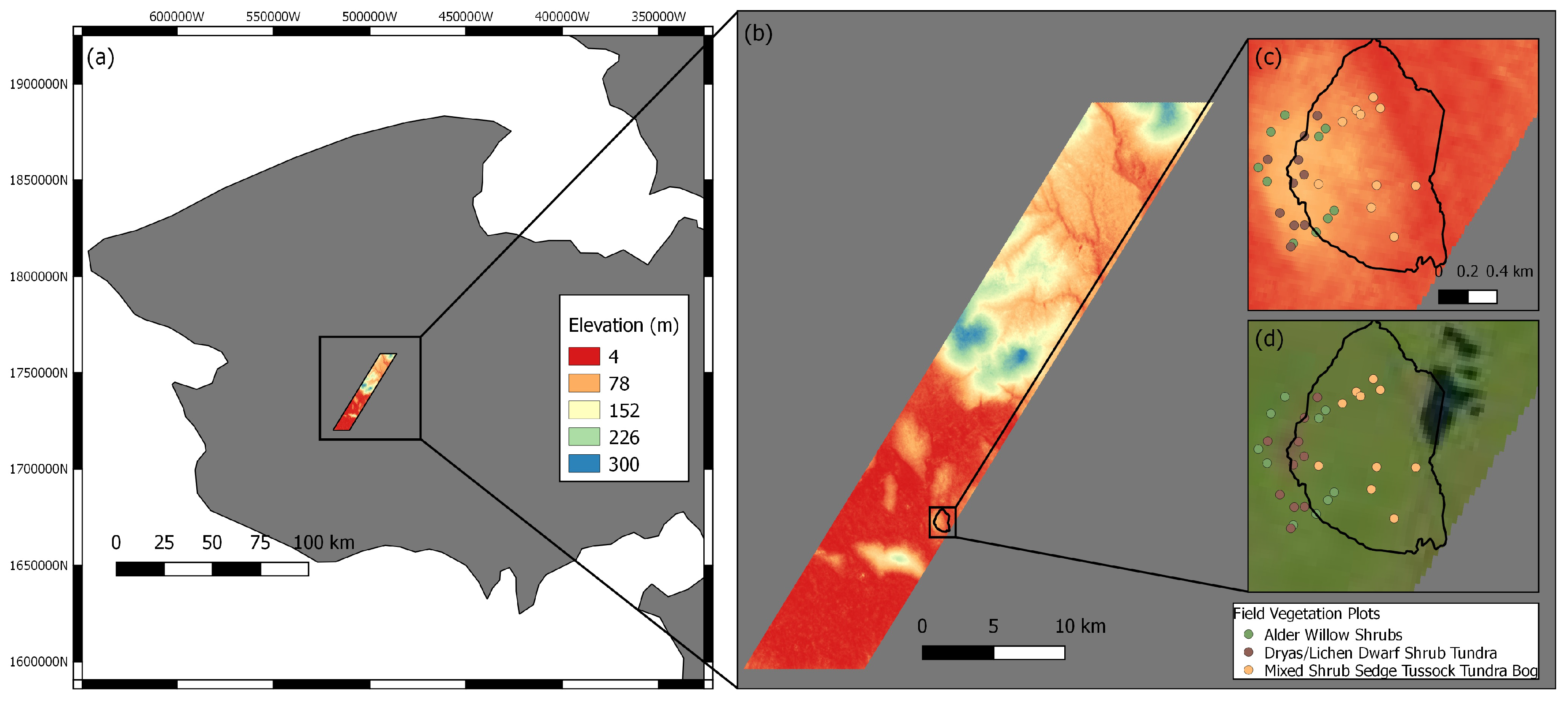
DEM over the study area located on the Seward Peninsula (a), shown in the right panel (b) is the study area showing the Kougarok watershed (black boundary). The Kougarok watershed is shown with the field vegetation plot locations (colored circles) with the DEM (c) and Landsat 8 OLI true color image (d).
Figure 1.
DEM over the study area located on the Seward Peninsula (a), shown in the right panel (b) is the study area showing the Kougarok watershed (black boundary). The Kougarok watershed is shown with the field vegetation plot locations (colored circles) with the DEM (c) and Landsat 8 OLI true color image (d).

Figure 2.
Workflow for the processing of the remote sensing datasets and development of vegetation classifications. Image processing and fusion is described in Section 3.1. CNN model preparation is discussed in Section 3.3. Two sets of CNN models were created: (1) trained using the labels from the Alaska Existing Vegetation Type (AKEVT; http://akevt.gina.alaska.edu/) map and (2) trained using the labels from unsupervised clustering based vegetation map (discussed in Section 3.2). Validation is discussed in Section 3.4.

Figure 3.
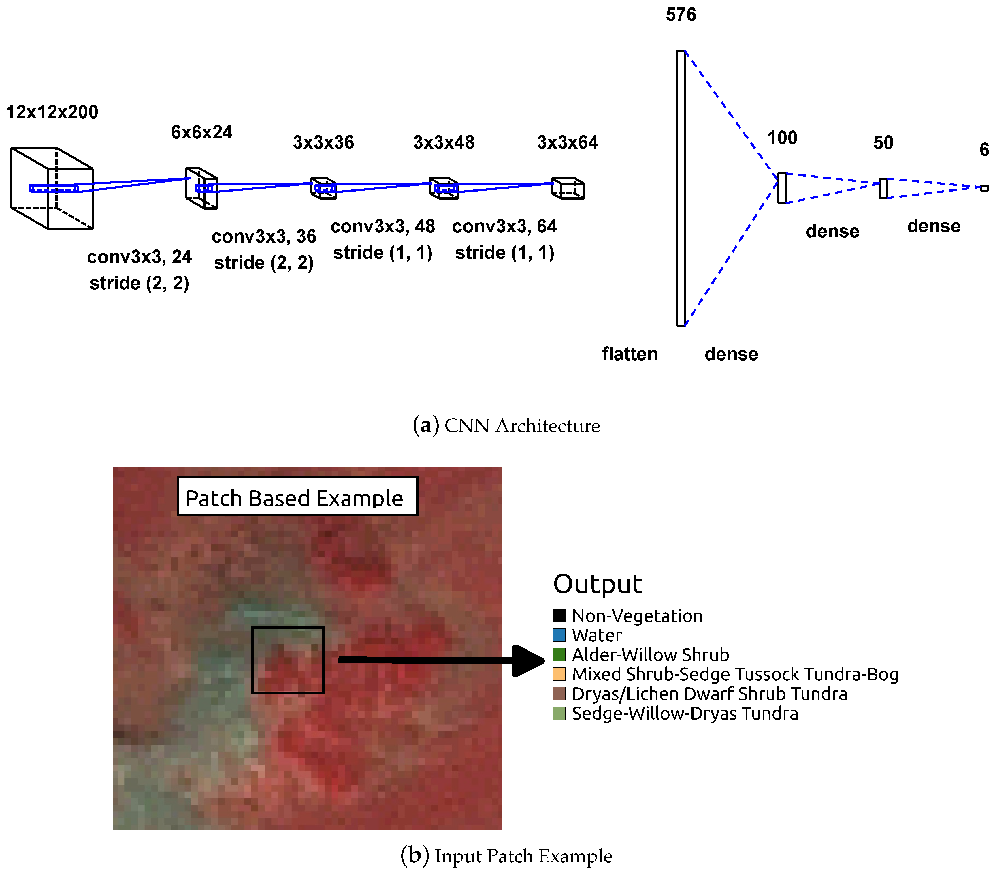
(a) CNN architecture used in the study, showing an example 12 × 12 image patch (with 200 bands) presented as the input. This is convolved with 24 different 1st layer filters, with a kernel size of 3 × 3, using a stride of 2. Similar operations are repeated linearly in the following layers, increasing the filter size as the image patch decreases in size. The last three layers are fully connected, taking features from the top convolutional layer as inputs. The final layer is a softmax function, corresponding to the number of vegetation classes (6). (b) Example 12 × 12 image patch input into the CNN with the output corresponding to a single label.
Figure 3.
(a) CNN architecture used in the study, showing an example 12 × 12 image patch (with 200 bands) presented as the input. This is convolved with 24 different 1st layer filters, with a kernel size of 3 × 3, using a stride of 2. Similar operations are repeated linearly in the following layers, increasing the filter size as the image patch decreases in size. The last three layers are fully connected, taking features from the top convolutional layer as inputs. The final layer is a softmax function, corresponding to the number of vegetation classes (6). (b) Example 12 × 12 image patch input into the CNN with the output corresponding to a single label.

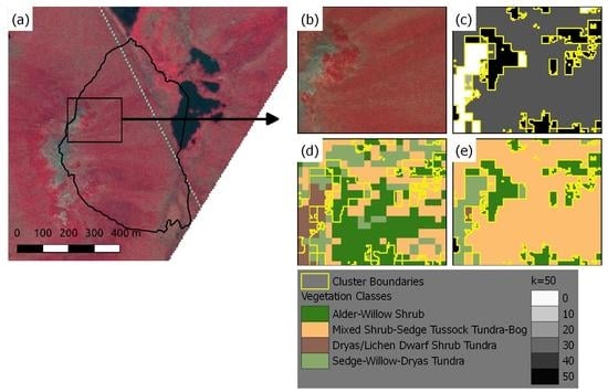
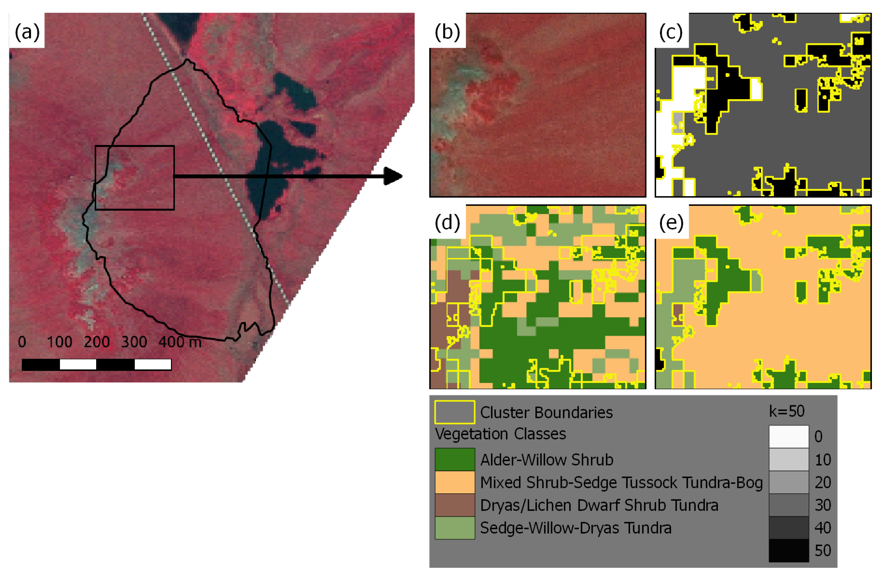
Figure 4.
(a) Example graphic of the UCVM method over the Kougarok watershed, with a zoomed in view of a specific region of the SPOT-5 false color image (b). (c) Clustering applied to the input remote sensing variables, with the four clusters (white, black, light gray, and dark gray) outlined in yellow. (d) Overlap of the clusters to the AKEVT map and (e) reclassed clusters based on the GOF score.

Figure 5.
(a) Unsupervised classification map (k = 50) of the study region using multi-sensor dataset. (b) The AKEVT map for the study region. (c) The UCVM map of the study region based on unsupervised clustering. (d) Map showing the GOF scores for UCVM-k50 across the study region. (e) Unsupervised cluster (k = 50) map of the Kougarok watershed. (f) The AKEVT map for the Kougarok watershed. (g) The UCVM-k50 map for the Kougarok watershed based on unsupervised clustering. (h) The GOF scores map for UCVM within the Kougarok watershed. The circles represent the field datasets, color-coded for the vegetation class.

Figure 6.
Validation scores against the 30 field vegetation plots, AKEVT (a), UCVM-k10 (b), UCVM-k25 (c), and UCVM-k50 (d). The precision, recall, and f1-score scores are displayed by k value (e). (AW: Alder-Willow Shrub; DL: Dryas/Lichen Dwarf Shrub Tundra; MS: Mixed Shrub-Sedge Tussock Tundra-Bog; NV: Non-Vegetated; SW: Sedge-Willow-Dryas Tundra, and W: Water).

Figure 7.
Spectral characteristics of the EO-1 Hyperion dataset (400–2500 nm) for each vegetation class from the for the AKEVT (a) and UCVM (b) maps, showing spectral differences described in Section 4.2. Solid lines and shaded curves show the mean and 90th percentile distribution of values across the classes respectively. The masked out regions consists of the non-calibrated bands.

Figure 8.
Box-plots representing variability of Landsat 8 (L8 B1–B9) TOA values, SPOT-5 data (green, red, NIR) normalized values, and IfSAR DSM normalized values for the AKEVT (a) and UCVM (b) maps, showing spectral differences described in Section 4.2. The values were segregated by vegetation type, where AW, DL, MS, NV, SW, and W stand for Alder-Willow Shrub, Dryas/Lichen Dwarf Shrub Tundra, Mixed Shrub-Sedge Tussock Tundra-Bog, Non-Vegetated, Sedge-Willow-Dryas Tundra, and Water, respectively.

Figure 9.
CNN model convergence over 100 epochs for patch size of 3 × 3, 6 × 6, and 12 × 12 when trained using AKEVT (a–c), and UCVM (d–f), where the green line indicates the test dataset and the blue line indicates the training dataset. Notice the CNN-AKEVT model overfits for the 6 × 6 and 12 × 12 image patches after certain epochs.

Figure 10.
Validation statistics using field based vegetation observations for the CNN models trained using the UCVM dataset. (AW: Alder-Willow Shrub; DL: Dryas/Lichen Dwarf Shrub Tundra; MS: Mixed Shrub-Sedge Tussock Tundra-Bog; NV: Non-Vegetated; SW: Sedge-Willow-Dryas Tundra, and W: Water. avg: average score; wtmean: area weighted mean score.)

Figure 11.
Validation statistics using field based vegetation observations for the CNN models trained using AKEVT dataset. (AW: Alder-Willow Shrub; DL: Dryas/Lichen Dwarf Shrub Tundra; MS: Mixed Sedge-Willow-Dryas Tundra, and W: Water. avg: average score; wtmean: area weighted mean score.)
Figure 11.
Validation statistics using field based vegetation observations for the CNN models trained using AKEVT dataset. (AW: Alder-Willow Shrub; DL: Dryas/Lichen Dwarf Shrub Tundra; MS: Mixed Sedge-Willow-Dryas Tundra, and W: Water. avg: average score; wtmean: area weighted mean score.)

Figure 12.
(a) Vegetation map over the field plots using the 6 × 6 patch CNN-UCVM model and (b) SPOT 5 false color image.
Figure 12.
(a) Vegetation map over the field plots using the 6 × 6 patch CNN-UCVM model and (b) SPOT 5 false color image.

Figure 13.
Validation statistics using field vegetation observations in the Kougarok watershed for (a) AKEVT, (b) UCVM, (c) CNN-UCVM (6 × 6), (d) CNN-AKEVT (3 × 3). (AW: Alder-Willow Shrub; DL: Dryas/Lichen Dwarf Shrub Tundra; MS: Mixed Shrub-Sedge Tussock Tundra-Bog; NV: Non-Vegetated; SW: Sedge-Willow-Dryas Tundra, and W: Water. avg: average score; wtmean: area weighted mean score.)


Table 1.
Area (km2) of the AKEVT vegetation classes within the study region (SR) and the Kougarok watershed (KW). The crosswalk between AKEVT and AATVM types, number of plots within each vegetation type, and the size of field plots by vegetation type are also presented. Field samples were not collected for Sedge-Willow-Dryas Tundra, Non-Vegetated, and Water classes.
| AKEVT Class | SR Area | KW Area | AATVM Class | Samples | Plot Size |
|---|---|---|---|---|---|
| Alder-Willow Shrub | 72.38 | 0.57 | Alder Shrubland | 5 | 5 × 5 m |
| Willow-Birch Tundra | 5 | 2.5 × 2.5 m | |||
| Mixed Shrub-Sedge Tussock Tundra-Bog | 117.61 | 0.45 | Tussock Tundra | 5 | 2.5 × 2.5 m |
| Shrubby Tussock Tundra | 5 | 2.5 × 2.5 m | |||
| Dryas/Lichen Dwarf Shrub Tundra | 20.02 | 0.15 | Dwarf Shrub Lichen Tundra | 5 | 2.5 × 2.5 m |
| Non-acidic Mountain Complex | 5 | 2.5 × 2.5 m | |||
| Sedge-Willow-Dryas Tundra | 113.34 | 0.54 | |||
| Non-Vegetated | 5.53 | 0.007 | |||
| Water | 6.00 | 0.02 |
Table 2.
Spectral and topographic variables used in the optical- and SAR-derived classifications, where DN stands for Digital Numbers.
Table 2.
Spectral and topographic variables used in the optical- and SAR-derived classifications, where DN stands for Digital Numbers.
| Sensor Group | Predictor Variable | Unit | Collection Date | Resolution |
|---|---|---|---|---|
| SPOT-5 | Green, Red, NIR (0.5–0.9 μm) | DN | June–September 2009–2012 | 2.5 m |
| DSM | Elevation | meter | July 2012 | 5 m |
| EO-1 | 198 spectral bands (0.4–2.5 μm) | DN | 24 June 2015 | 30 m |
| Landsat 8 | 9 spectral bands (0.4–2.29 μm) | DN | 17 August 2016 | 30 m |
Table 3.
Area distribution of vegetation classes for UCVM map based on k = 50 within the entire study region and the Kougarok watershed.
Table 3.
Area distribution of vegetation classes for UCVM map based on k = 50 within the entire study region and the Kougarok watershed.
| AKEVT Land Cover | Study Region Area (km2) | Kougarok Watershed Area (km2) |
|---|---|---|
| Alder-Willow Shrub | 73.33 | 0.55 |
| Mixed Shrub-Sedge Tussock Tundra-Bog | 135.27 | 0.58 |
| Dryas/Lichen Dwarf Shrub Tundra | 14.88 | 0.07 |
| Sedge-Willow-Dryas Tundra | 102.14 | 0.50 |
| Non-Vegetated | 2.24 | 0.02 |
| Water | 7.04 | 0.04 |
| Total | 334.89 | 1.75 |
© 2019 by the authors. Licensee MDPI, Basel, Switzerland. This article is an open access article distributed under the terms and conditions of the Creative Commons Attribution (CC BY) license (http://creativecommons.org/licenses/by/4.0/).
Share and Cite
MDPI and ACS Style
Langford, Z.L.; Kumar, J.; Hoffman, F.M.; Breen, A.L.; Iversen, C.M. Arctic Vegetation Mapping Using Unsupervised Training Datasets and Convolutional Neural Networks. Remote Sens. 2019, 11, 69. https://doi.org/10.3390/rs11010069
AMA Style
Langford ZL, Kumar J, Hoffman FM, Breen AL, Iversen CM. Arctic Vegetation Mapping Using Unsupervised Training Datasets and Convolutional Neural Networks. Remote Sensing. 2019; 11(1):69. https://doi.org/10.3390/rs11010069
Chicago/Turabian StyleLangford, Zachary L., Jitendra Kumar, Forrest M. Hoffman, Amy L. Breen, and Colleen M. Iversen. 2019. "Arctic Vegetation Mapping Using Unsupervised Training Datasets and Convolutional Neural Networks" Remote Sensing 11, no. 1: 69. https://doi.org/10.3390/rs11010069
Note that from the first issue of 2016, this journal uses article numbers instead of page numbers. See further details here.