Dense Semantic Labeling with Atrous Spatial Pyramid Pooling and Decoder for High-Resolution Remote Sensing Imagery

Abstract

Dense semantic labeling is significant in high-resolution remote sensing imagery research and it has been widely used in land-use analysis and environment protection. With the recent success of fully convolutional networks (FCN), various types of network architectures have largely improved performance. Among them, atrous spatial pyramid pooling (ASPP) and encoder-decoder are two successful ones. The former structure is able to extract multi-scale contextual information and multiple effective field-of-view, while the latter structure can recover the spatial information to obtain sharper object boundaries. In this study, we propose a more efficient fully convolutional network by combining the advantages from both structures. Our model utilizes the deep residual network (ResNet) followed by ASPP as the encoder and combines two scales of high-level features with corresponding low-level features as the decoder at the upsampling stage. We further develop a multi-scale loss function to enhance the learning procedure. In the postprocessing, a novel superpixel-based dense conditional random field is employed to refine the predictions. We evaluate the proposed method on the Potsdam and Vaihingen datasets and the experimental results demonstrate that our method performs better than other machine learning or deep learning methods. Compared with the state-of-the-art DeepLab_v3+ our model gains 0.4% and 0.6% improvements in overall accuracy on these two datasets respectively.

1. Introduction

High-resolution remote sensing imagery captured by satellite or unmanned aerial vehicle (UAV) contains rich information and is significant in many applications, including land-use analysis, environment protection and urban planning [1]. Due to the rapid development of remote sensing technology, especially the improvement of imaging sensors, a massive number of high-quality images are available to be utilized [2]. With the support of sufficient data, dense semantic labeling, also known as semantic segmentation in computer vision, is now an essential aspect in research and is playing an increasingly critical role in many applications [3].

To better understand the scene, dense semantic labeling aims at segmenting the objects of given categories from the background of the images at the pixel-level, such as buildings, trees and cars [4]. In the past decades, a vast number of algorithms have been proposed. These algorithms can be divided into two major parts, that is, traditional machine learning methods and convolutional neural network (CNN) methods [5].

Traditional machine learning methods usually adopt a two-stage architecture consisting of a feature extractor and a classifier [6]. The feature extractor aims at extracting spatial and textural features from local portions of the image, encoding the spatial arrangements of pixels into a high-dimensional representation [7]. Many powerful feature extractors have been presented before, such as Histogram of oriented gradients (HOG) [8], Scale invariant Feature Transform (SIFT) [9] and Speeded up robust features (SURF) [10]. Meanwhile, the classifier makes the prediction of every pixel in the image based on the extracted features. Support vector machines [11], Random forests [12] and K-means [13] are usually employed. However, these traditional machine learning methods cannot achieve a satisfactory result, due to massive changes in illumination in the images and the strong similarity of shape and color with different categories of objects. It is challenging to have a robust prediction [14].

In recent years, convolutional neural networks have achieved extreme success in many domains of computer vision tasks, including dense semantic labeling [15,16]. CNNs learn the network parameters directly from data using backpropagation and have more hidden layers which means a more powerful nonlinear fitting ability [17]. In the early stage, CNNs focused on classification tasks, significantly outperformed the traditional machine learning methods on ImageNet large scale visual recognition competition (ILSVRC) [18]. Afterwards, many excellent networks were proposed, such as VGG [19], Deep residual network (ResNet) [20] and DenseNet [21]. However, dense semantic labeling is a pixel-level classification task [22]. To retain the spatial structure, fully convolutional networks (FCN) [23] replace the fully connected layers with upsampling layers. Through the upsampling operations, the downsampled feature maps can be restored to the original resolution of the input image. The FCN model is the first end-to-end, pixels-to-pixels network and most further networks are based on it [24].

Nowadays, the classification accuracy of FCN-based models is relatively high. The primary objective in dense semantic labeling tasks is to obtain a more accurate boundary of objects and deal with the misclassification problem of small objects. The challenge comes from two aspects. First, the pooling layers or convolution striding used between convolution layers can augment the receptive field; meanwhile, they can also downsample the resolution of feature maps which cause the loss of spatial information. Second, objects of the same category exist in multiple scales of shape and small objects are hard to classify correctly [25]. Therefore, simply employing upsampling operations such as deconvolution or bilinear interpolation after the feature extractor parts of a network cannot guarantee a fine prediction result. Many network structures have been proposed to handle these problems; among them, atrous spatial pyramid pooling (DeepLab) [26] and encoder-decoder (U-net) [27] are the state-of-art structures.

The atrous spatial pyramid pooling (ASPP) network structure from the DeepLab model has been well-known for achieving robust and efficient dense semantic labeling performance and it aims at handling the problem of segmenting objects at multiple scales [28]. The network structure consists of several branches of atrous convolution operations and each branch has a different rate of the convolution kernels to probe an incoming feature map at specific effective field-of-view. Therefore, ASPP shows better performance on detecting objects at different scales of shape, especially the small objects. But DeepLab model only utilized a simple bilinear interpolation after ASPP to restore the resolution of feature maps that lead to a bad impact on getting fine boundary of the objects.

The encoder-decoder structure from U-net has been widely used in the dense semantic labeling tasks of remote sensing imageries [14,29]. It adopts several skip connections between top layers and bottom layers at the upsampling stage. Due to the combination of contextual information at scales of 1, $1/2$, $1/4$, $1/8$ of the input resolution, spatial information damaged by the pooling operations can be better restored, so objects in the final prediction have a sharper boundary after the decoder. However, U-net has no consideration for the extraction of multiple scales of features.

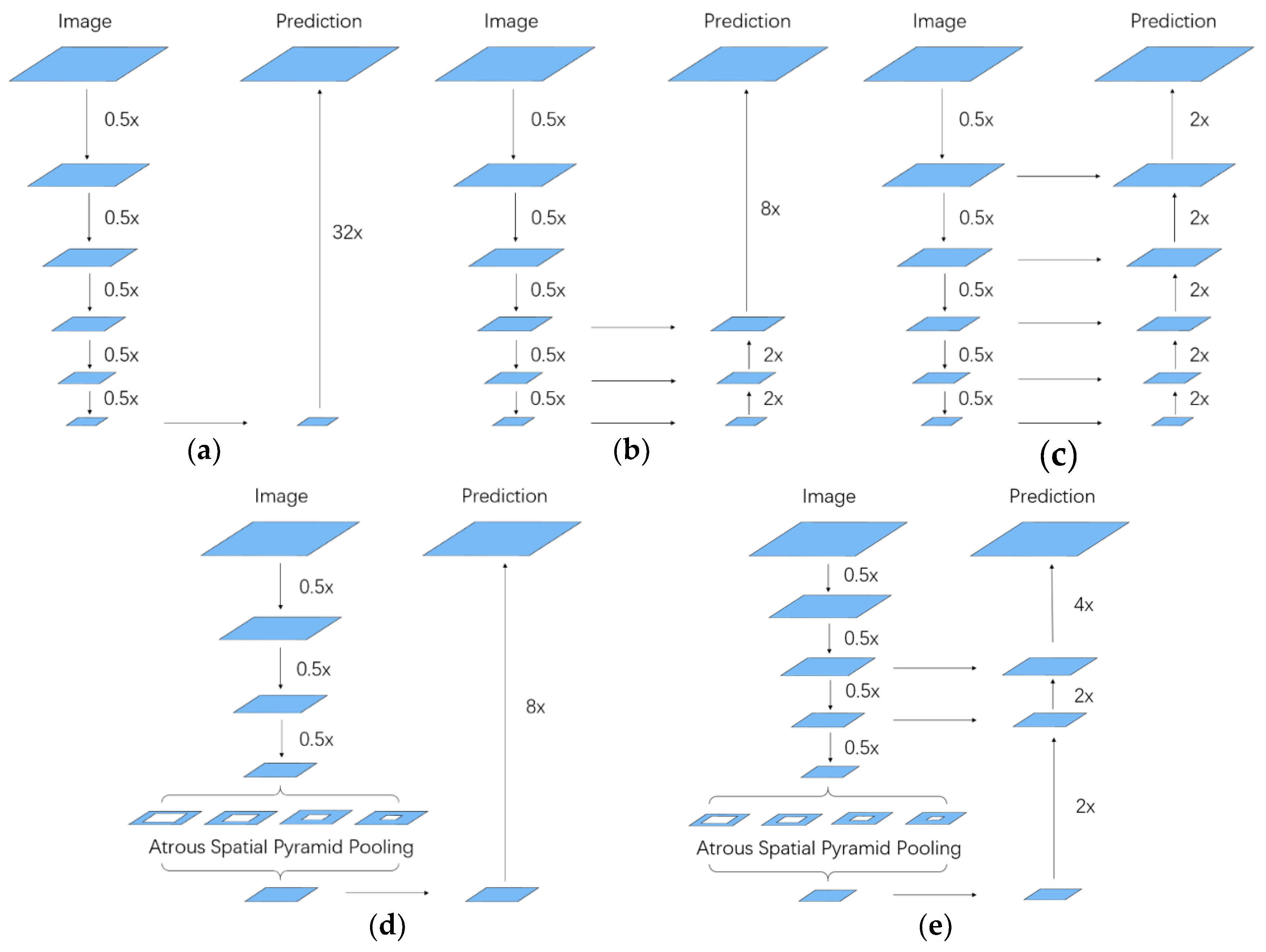
These two powerful network structures only focus on the two problems in dense semantic labeling respectively and no works have taken them into account simultaneously before. Therefore, a model employing both of them could further improve the performance. Figure 1 shows details of alternative network structures of dense semantic labeling.

Inspired by the analysis above, we propose a novel architecture of the fully convolutional network that aims at not only detecting objects of different shapes but also restoring sharper object boundaries simultaneously. Our model adopts the deep residual network (ResNet) as the backbone, followed by atrous spatial pyramid pooling (ASPP) structure to extract multi-scale contextual information; these two parts constitute the encoder. Then we design the decoder structures by fusing two scales of low-level feature maps from ResNet with the corresponding predictions to restore the spatial information. To make this two structure fusion effective, we append a multi-scale softmax cross-entropy loss function with corresponding weights at the end of networks. Different from the loss function in Reference [29], our proposed loss function guides every scale of prediction during the training procedure which helps better optimize the parameters in the intermediate layers. After the networks, we improve the dense conditional random field (DenseCRF) using a superpixel algorithm in post-processing that gives an additional boost to performance. Experiments on the Potsdam and Vaihingen datasets demonstrate that our model outperformed other state-of-art networks and achieved 88.4% and 87.0% overall accuracy respectively with the calculation of the boundary pixels of objects. The main contributions of our study are listed as follows:

• We propose a novel convolutional neural network that combines the advantages of ASPP and encoder-decoder structures.
• We enhance the learning procedure by employing a multi-scale loss function.
• We improve the dense conditional random field with a superpixel algorithm to optimize the prediction further.

The remainder of this paper is organized as follows: Section 2 describes our dense semantic labeling system which includes the proposed model and the superpixel-based DenseCRF. Section 3 presents the datasets, preprocessing methods, training protocol and results. Section 4 is the discussion of our method and Section 5 concludes the whole study.

2. Methods

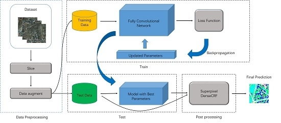
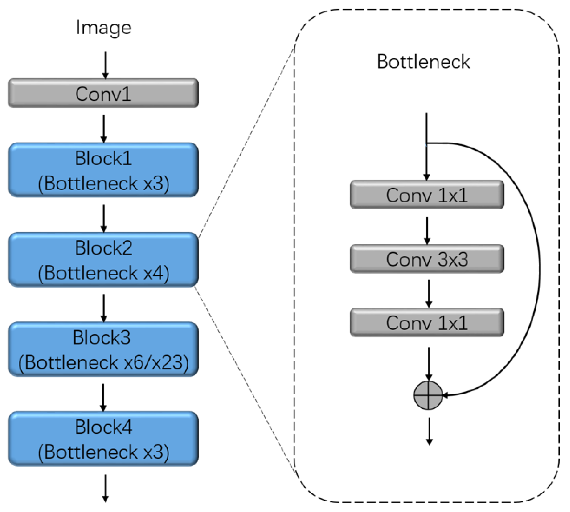
In this paper, a dense semantic labeling system to extract categorized objects from high-resolution remote sensing imagery is proposed. The system involves in the following stages. First, the imageries including red, green, blue (RGB), infrared radiation (IR) and normalized digital surface model (DSM) channels and groundtruth are sliced into small patches to generate the training and test data. Meanwhile, some data augmentation methods are employed to increase the complexity of data, such as flipping and rescaling the imageries randomly and so forth. Then, our proposed fully convolutional network is trained using the training data; the training procedure is based on the gradient descent algorithm that uses the updated parameters calculated by the loss function to improve the performance of the network. After that, the trained model with the best parameters will be chosen to generate predictions on the test data. Finally, we introduce a superpixel-based DenseCRF to optimize the predictions further. The pipeline of our dense semantic labeling system is illustrated in Figure 2.

2.1. Encoder with ResNet and Atrous Spatial Pyramid Pooling

In this section, we introduce the encoder part of the proposed fully convolutional network. Our model adopts ResNet as the backbone, followed by the atrous spatial pyramid pooling structure. These two parts constitute the encoder to extract multiple scales of contextual information.

2.1.1. ResNet-101 as the Backbone

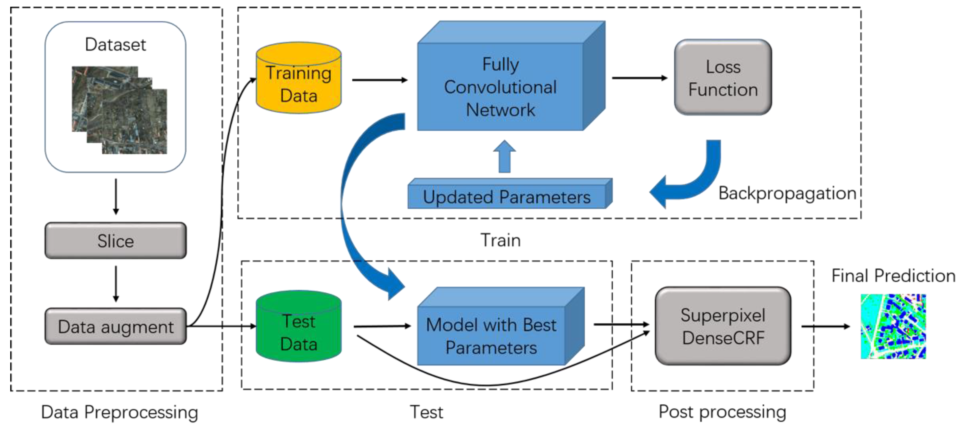
The backbone is the basic structure to extract features from input imageries in FCN-based models [30]. Nowadays, most works adopt classic classification networks such as VGG, ResNet without the fully connected parts. The reason is two-fold. First, these networks have excellent performance on ImageNet large scale visual recognition competition. Second, we can fine-tune our network with the pre-trained model. In this study, we choose ResNet as the backbone of our model. ResNet solved the vanishing-gradient problem [31] by employing the bottleneck unit and achieved better accuracy and smaller model size with deeper layers. Figure 3 shows details of ResNet and the bottleneck unit.

2.1.2. Atrous Spatial Pyramid Pooling

In this study, we utilize ASPP after ResNet to extract multi-scale contextual information further. ASPP is a parallel structure of several branches that operate to the same feature map and fuse the outputs in the end and it was first introduced in DeepLab_v2 network. ASPP employs the atrous convolution [32] in each branch. Different from standard convolution, atrous convolution has a rate parameter which adds the corresponding quantity of zeros between the parameters in the convolution filter. This operation equals the downsampling, convolution and upsampling process but has much better performance without increasing the number of parameters that maintains the efficiency of the network. The ASPP structure has two versions. The original one in DeepLab_v2 includes four branches of atrous convolution with rate 6, 12, 18, 24. But the convolution filter with rate 24 is close to the size of input feature maps, only the center of it takes effect. In DeepLab_v3 [33], it was replaced by a 1 × 1 convolution. Moreover, an image pooling branch is also appended to incorporate global context information. In our model, we employ the advanced ASPP structure.

2.2. Decoder and the Multi-scale Loss Function

In this section, we introduce the decoder part of our model. Based on the encoder structure mentioned above, we propose a two-step decoder structure at the upsampling stage to refine the boundary of objects in the final predictions and fuse the ASPP and encoder-decoder structure together. We also present a multi-scale loss function to solve the optimization problem caused by an excessive number of intermediate layers and to make the whole network more effective.

2.2.1. Proposed Decoder

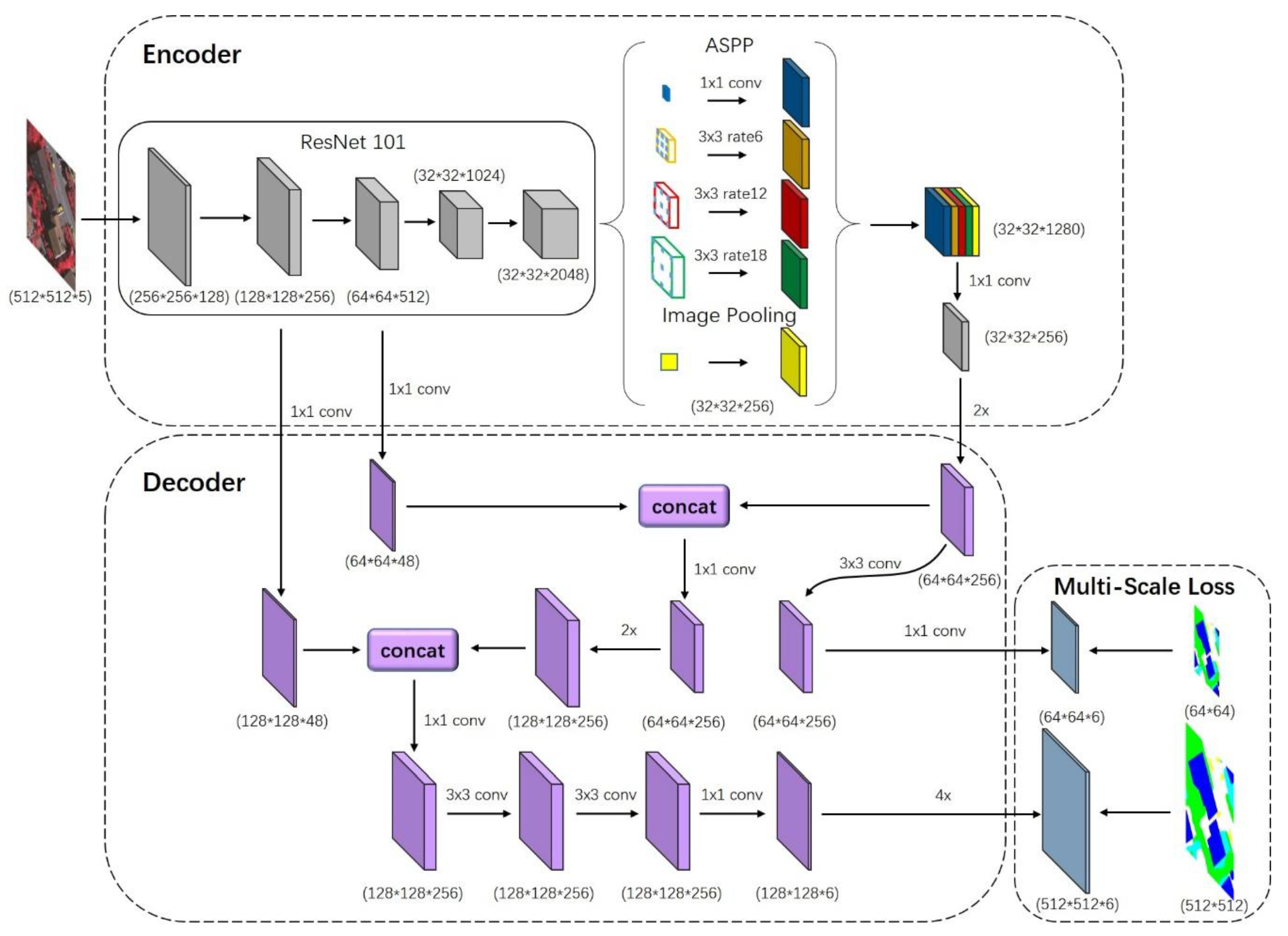
The decoder structure is to restore the spatial information and improve the final prediction by fusing the multi-scale high-level features with the corresponding scales of low-level features at the upsampling stage. In our model, the resolution of feature maps extracted by ResNet and ASPP is 16 times smaller than the input imageries. Here we propose a two-step decoder structure to restore the feature maps to the original resolution with the fusion of features from ResNet. First, the features maps from the encoder are bilinearly upsampled by a factor of 2 and concatenated with the corresponding low-level features in ResNet that have the same resolution (Conv1 of Bottleneck4 in Block2). Meanwhile, to prevent the corresponding low-level features (512 channels) from outweighing the importance of the high-level encoder features (only 256 channels), we apply a $1\times 1$ convolution to reduce the number of channels to 48. After the concatenation, another $1\times 1$ convolution is applied to reduce the number of channels to 256. Then we repeat this process to concatenate the lower-level features in ResNet (Conv1 of Bottleneck3 in Block1). In the end, two $3\times 3$ convolutions and one $1\times 1$ convolution are applied to refine the features followed by a bilinear upsampling by a factor of 4. Figure 4 shows details of our decoder structure.

2.2.2. Multi-scale Loss Function

The loss function is a necessary component in the deep learning model to calculate the deviation value between the prediction and groundtruth and optimize the parameters through backpropagation. Traditional FCN-based models adopt a single softmax cross-entropy loss function at the end of the network. For our model, we adopt the encoder structure which consists of ResNet101 and ASPP and propose a decoder structure of two-scale low-level features fusion. There is a large number of intermediate layers and their corresponding parameters, so one single loss function [34] is insufficient to optimize all the layers especially the layers in the encoder part (far from the loss function). To solve this, we apply a multi-scale softmax cross-entropy loss function at different scales of prediction. First, we append a loss function at the end of the network after the 4 times upsampling with the groundtruth of the original resolution. Then, we apply a $3\times 3$ convolution followed by $1\times 1$ convolution to the 2 times upsampled feature maps from ASPP and append another loss function with the 8 times downsampled groundtruth. The former loss function at the end guides the whole network training as the traditional method, while the latter one in the middle can further enhance the optimization of the parameters in the encoder. We also put corresponding weights for these two losses as ${\lambda }_1$ and ${\lambda }_2$. The overall loss function is:

$$L_{overall}={\lambda }_1\times L_{sub1}+{\lambda }_2\times L_{sub2}$$

(1)

During the training phase, our model is trained by the stochastic gradient descent (SGD) algorithm [35] to minimize the overall loss. The best performance was achieved using ${\lambda }_1=0.5$ and ${\lambda }_2=0.5$. As more constraints were applied, the ASPP and encoder-decoder structure fusion could be more effective. The multi-scale loss function is shown in Figure 4 and the detailed configurations of the proposed network is shown in

Table 1. Configurations of the proposed network.

	Layer	Type	Kernel Size	Resolution	Connect to
ResNet 101	conv_1	convolution	$3\times 3$, 128	$256\times 256$	block1
	block1	residual_block $\times 3$	-, 256	$128\times 128$	block2 & conv2_2
	block2	residual_block $\times 4$	-, 512	$64\times 64$	block3 & conv1_2
	block3	residual_block $\times 23$	-, 1024	$32\times 32$	block4
	block4	residual_block $\times 3$	-, 2048	$32\times 32$	ASPP
ASPP	branch1	convolution	$1\times 1$, 256	$32\times 32$	concat_1
	branch2	atrous_conv	$3\times 3$, rate = 6, 256	$32\times 32$	concat_1
	branch3	atrous_conv	$3\times 3$, rate = 12, 256	$32\times 32$	concat_1
	branch4	atrous_conv	$3\times 3$, rate = 18, 256	$32\times 32$	concat_1
	branch5	global_pooling	-, 256	$32\times 32$	concat_1
	concat_1	concatenation	-, 1280	$32\times 32$	conv1_1
	conv1_1	convolution	$1\times 1$, 256	$32\times 32$	up_1
Decoder	up_1	upsample	-, 256	$64\times 64$	concat_2 & conv1_3
	conv1_2	convolution	$1\times 1$, 48	$64\times 64$	concat_2
	conv1_3	convolution	$3\times 3$, 256	$64\times 64$	conv1_4
	conv1_4	convolution	$1\times 1$, 6	$64\times 64$	$L_{sub1}$
	concat_2	concatenation	-, 304	$64\times 64$	conv2_1
	conv2_1	convolution	$1\times 1$, 256	$64\times 64$	up_2
	up_2	upsample	-, 256	$128\times 128$	concat_3
	conv2_2	convolution	$1\times 1$, 48	$128\times 128$	concat_3
	concat_3	concatenation	-, 304	$128\times 128$	conv3_1
	conv3_1	convolution $\times 2$	$3\times 3$, 256	$128\times 128$	conv3_2
	conv3_2	convolution	$1\times 1$, 6	$128\times 128$	up_3
	up_3	upsample	-, 6	$512\times 512$	$L_{sub2}$

.

2.3. Dense Conditional Random Fields Based on Superpixel

For dense semantic labeling tasks, post-processing after the deep learning model is a common method to optimize the predictions additionally. The most widely used one is Dense Conditional Random Fields (CRF) [36,37]. As a graph theory-based algorithm, pixel-level labels can be considered as random variables and the relationship between pixels in the image can be considered as edges, these two factors constitute a conditional random field. The energy function employed in CRF is:

$$E\left(x\right)={\displaystyle \sum _i{\theta }_i\left(x_i\right)+{\displaystyle \sum _{ij}{\varphi }_{ij}\left(x_i,x_j\right)}}$$

(2)

where $x$ is the label for the pixels in input image, ${\theta }_i\left(x_i\right)$ is the unary potential that represents the probability at pixel $i$ and ${\varphi }_{ij}\left(x_i,x_j\right)$ is the pairwise potentials that represent the cost between labels $x_i$, $x_j$ at pixels $i$, $j$. The expression of pairwise potential is:

$${\varphi }_{ij}\left(x_i,x_j\right)=\mu \left(x_i,x_y\right)\left[{\omega }_1\exp \left(-\frac{{\Vert p_i-p_j\Vert }^2}{2{\sigma }_{\alpha }^2}-\frac{{\Vert I_i-I_j\Vert }^2}{2{\sigma }_{\beta }^2}\right)+{\omega }_2\exp \left(-\frac{{\Vert p_i-p_j\Vert }^2}{2{\sigma }_{\gamma }^2}\right)\right]$$

(3)

where $\mu \left(x_i,x_y\right)=1$ if $x_1\ne x_2$ and $\mu \left(x_i,x_y\right)=0$ otherwise, as shown in Potts model [38]. The other expressions are two Gaussian kernels. The first one represents both pixel positions and color, the second one represents only pixel positions. $I_i$ and $p_i$ are color vector and pixel position at pixel $i$.

The common inputs for CRF are prediction map and RGB image. In our study, we employ a superpixel algorithm (SLIC) [39,40] to boost the performance of CRF. Superpixel algorithm can segment the image into a set of patches and each patch consists of several pixels that are similar in color, location and so forth. The superpixel algorithm has the ability to detect the boundaries of the object in images. The process of our superpixel-based CRF is as follows:

Algorithm 1. The process of CRF based on superpixel

Input RGB image $I$ and prediction map from our model $L$. All the $J$ categories of object in dataset denoted as $C=\left\{c_1,c_2,\dots ,c_J\right\}$. Apply SLIC algorithm to $I$, generate $M$ superpixels $S=\left\{s_1,s_2,\dots ,s_M\right\}$, $s_i$ is the $i$ th superpixel region. Loop: For $i=1:M$ (1) All the $N$ pixels in $s_i$ denoted as $P_i=\left\{p_{i1},p_{i2},\dots ,p_{iN}\right\}$. (2) Each pixel $p_{ij}$ has a prediction $l_{ij}$ in $L$ and $l_{ij}\in C$, where $C$ is all the categories of object in dataset. (3) Count the number of predictions in every category, $\left\{count\left(c_1\right),count\left(c_2\right),\dots ,count\left(c_J\right)\right\}$. (4) The new prediction for the whole superpixel is ${\tilde{l}}_{s_i}=\max \left(count(c_1),count(c_2),\dots ,count\left(c_J\right)\right)$. End Update the prediction map as $\tilde{L}$. Apply DenseCRF to $I$ and $\tilde{L}$, output the final prediction $L_{final}$.

3. Results

3.1. Datasets

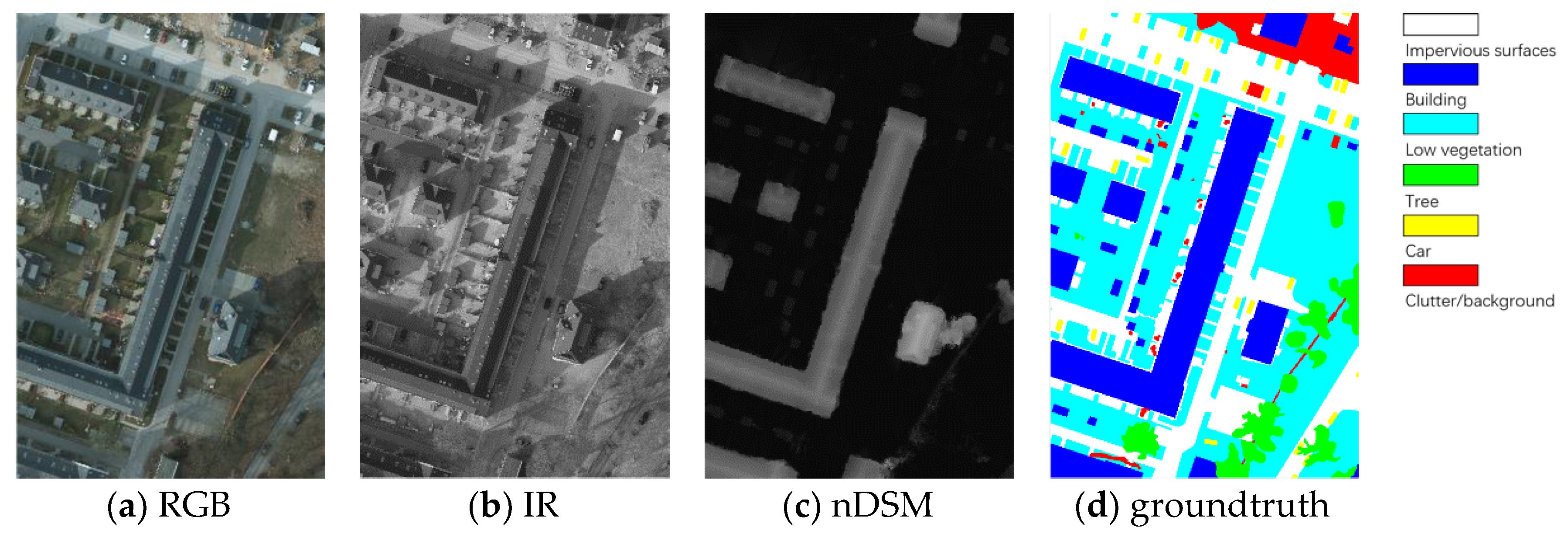
We evaluate our dense semantic labeling system on the ISPRS 2D high-resolution remote sensing imageries which include the Potsdam and Vaihingen datasets. These two datasets are open online (http://www2.isprs.org/commissions/comm3/wg4/semantic-labeling.html) and captured by airborne sensors with 6 categories: impervious surfaces (white), building (blue), low vegetation (cyan), tree (green), car (yellow), cluster/background (red). Their ground sampling distance are 5 cm and 9 cm. The Potsdam dataset contains 38 imageries with 5 channel data of red, green, blue, infrared and digital surface model (DSM) [41] at resolution of $6000\times 6000$; all the imageries have corresponding pixel-level groundtruth, 24 imageries are for training and 14 imageries are for testing. While the Vaihingen dataset includes 33 imageries with 4 channel data of red, green, infrared and DSM at approximate resolution of $2500\times 2500$. Similar to the Potsdam dataset, all the imageries have corresponding pixel-level groudtruth. 16 imageries are for training and 17 imageries are for testing. For DSM in these two datasets, we utilize the normalized DSM in our evaluation. Figure 5 shows a sample of the imagery.

3.2. Preprocessing the Datasets

All the imageries in datasets need be preprocessed before feeding to our model and the preprocessing operation consists of two parts, slicing and data augment.

The resolution of the imageries is too high. Due to the memory limit of the GPU hardware, feeding them directly to FCN-based model is impossible. To deal with this problem, there are two common methods, namely slicing and downsampling [42]. Downsampling will destroy the spatial structure of objects especially small size objects such as cars and low vegetation, so slicing is the better choice. In this study, according to the capacity of GPU memory, we slice the training imageries into $512\times 512$ patches with an overlay of 64 pixels (striding 448 pixels) and slice the test imageries with the same size without overlay.

Deep learning is a data-driven method, acquiring accurate results rely on the diversity and quality of the datasets. Data augment is an effective way to improve performance with the same amount of data [43]. In this study, we employ several specific methods. The problem of color imbalance, which is usually caused by the change of seasons and the incidence angle of sunlight has a significant influence in remote sensing imagery research. To solve this problem, we change the brightness, saturation hue and contrast randomly to augment the datasets. Object rotation is another problem to deal with. Unlike the general images, remote sensing imageries are captured in the air with different shooting angles. In order to solve it, we flip the imageries in horizontal and vertical directions randomly. For the problem of objects with multiple scales, we rescale the imageries from a factor of 0.5 to 2 and apply padding or cropping to restore the original resolution.

3.3. Training Protocol and Metrics

Our proposed model is deployed on the TensorFlow deep learning platform [44] with one NVIDIA GTX1080Ti GPU (11GB RAM). Because of the limit of memory, the batch size of input imageries is set to 6. For the learning rate, we have explored different policies, including fixed policy and step policy. The results show that ‘poly’ learning rate policy is the best one. The formula is:

$$learning\_rate=initial\_learning\_rate{\left(1-\frac{iteration}{max\_iteration}\right)}^{power}$$

(4)

where $initial\_learning\_rate=0.007$, $power=0.9$ and $max\_iteration=100000$ in this study. The training time of the proposed network is 21 hours. The optimizer that we employed is stochastic gradient descent (SGD) with a momentum of 0.9. Our post-processing method of superpixel-based DenseCRF was implemented based on Matlab and the open source PyDenseCRF package.

The metrics to evaluate our dense semantic labeling system involve 4 different criteria: overall accuracy (OA), $F_1$ score, precision and recall. They have the high frequency to be employed in the former works. The formula is as follows:

$$OA=\frac{TP+TN}{P+N}$$

(5)

$$precision=\frac{TP}{TP+FP}$$

(6)

$$recall=\frac{TP}{TP+FN}$$

(7)

$$F_1=2\times \frac{precision\times recall}{precision+recall}$$

(8)

where $P$ is the number of Positive samples, $N$ is the number of negative samples, $TP$ is the true positive, $FP$ is the false positive and $FN$ is the false negative.

3.4. Experimental Results

To better evaluate our Dense semantic labeling system, U-net, DeepLab_v3 and even the newest version DeepLab_v3+ [29] are adopted as the baseline for the comparison to our proposed model. Moreover, classic DenseCRF is employed to make a contrast with our superpixel-based DenseCRF. It should be noted that all of the metric scores are computed with the pixels of the object boundary.

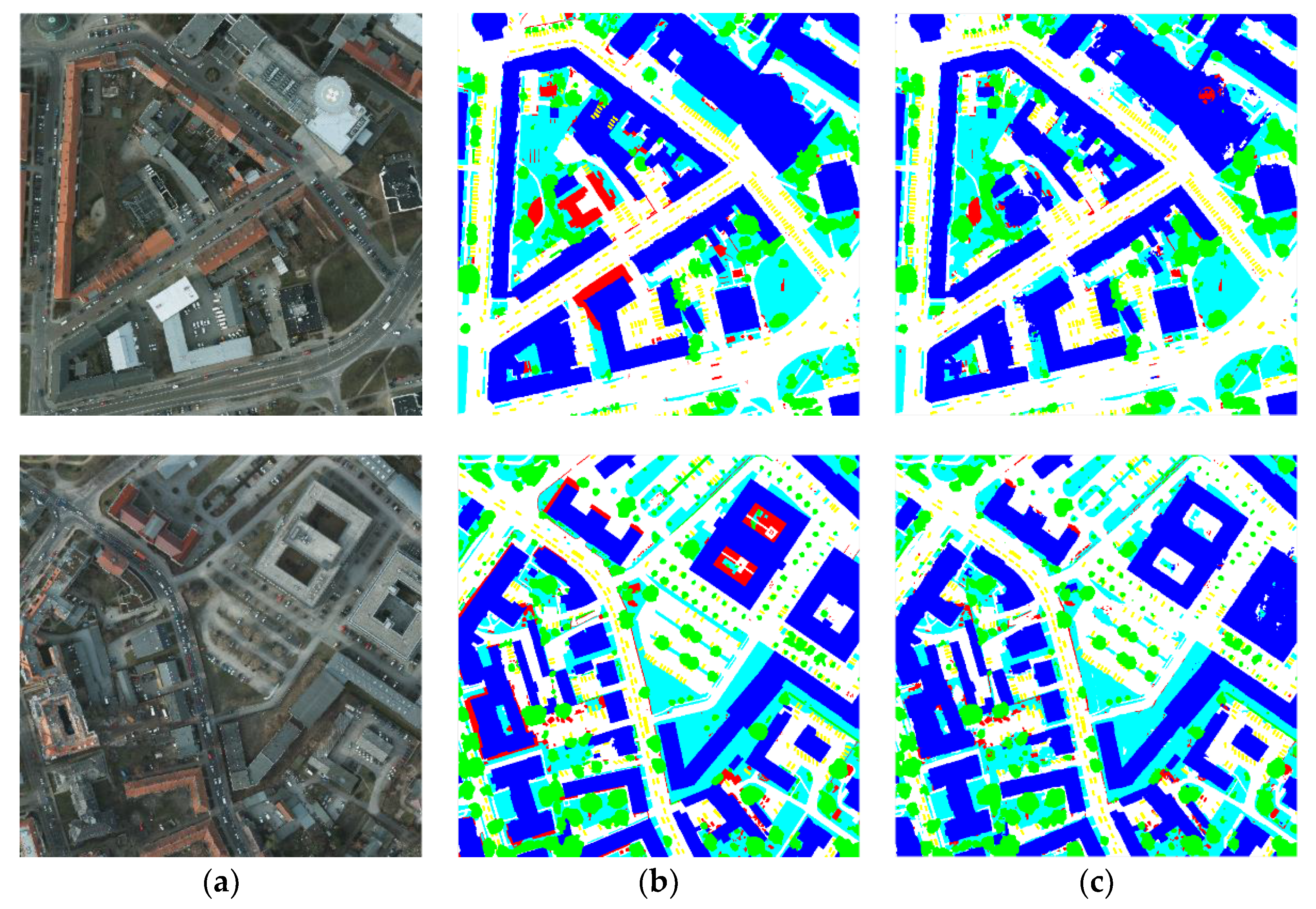
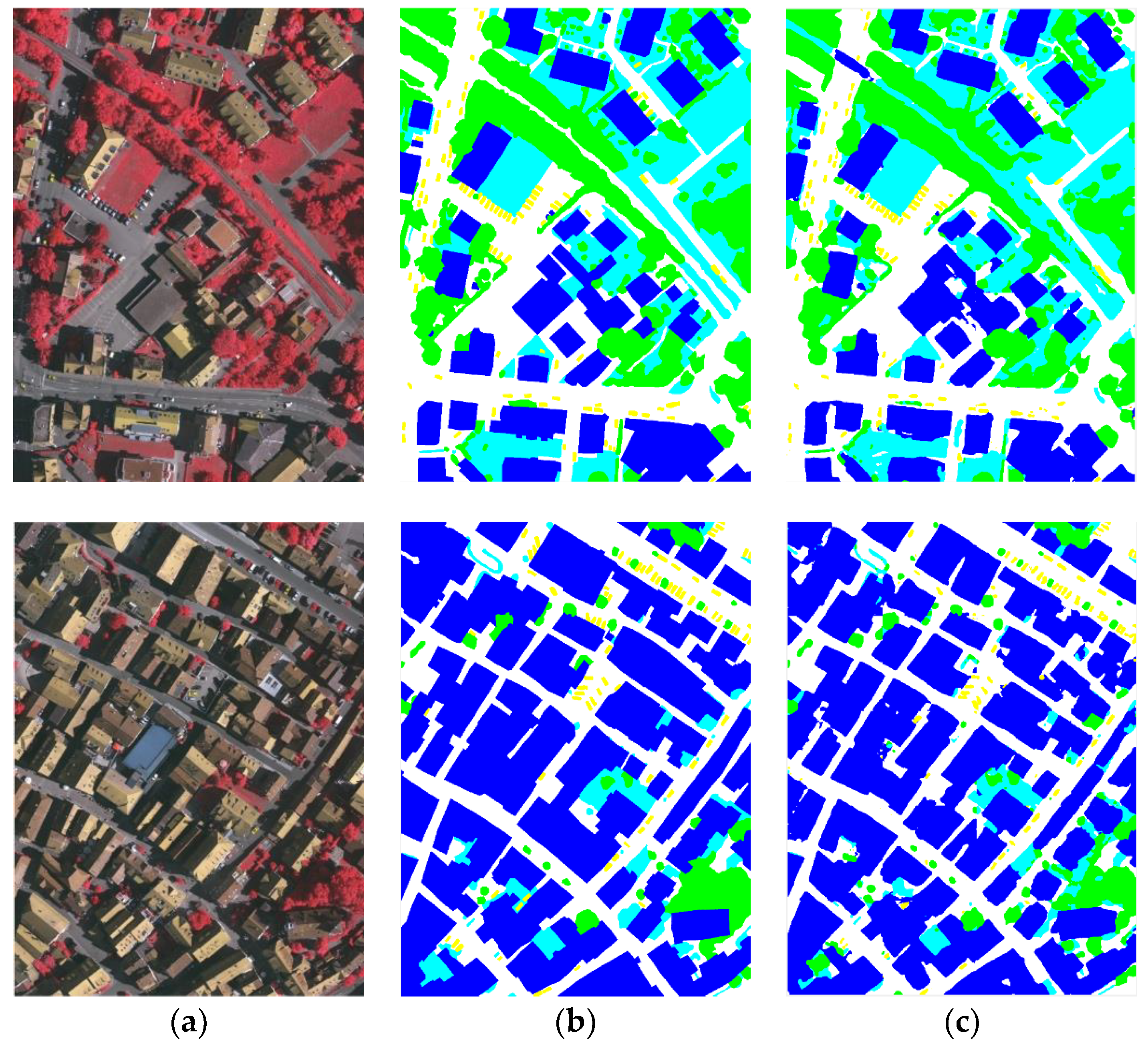
Our proposed model achieves 88.3% overall accuracy on the Potsdam dataset and 86.7% overall accuracy on the Vaihingen dataset. Figure 6 shows a sample of the result of our proposed model on the Potsdam dataset and Figure 7 shows a sample of the result on the Vaihingen dataset. The first column is the input high-resolution remote sensing imageries; the second column is their corresponding groudtruth; and the last column represents the prediction maps of our model. The detailed results in these two datasets are shown in

Table 2. The metric scores of overall accuracy, precision, recall, $F_1$ score for dense semantic labeling on the Potsdam dataset.

Metrics	Imp_surf	Building	Low_veg	Tree	Car	Average
OA	N/A	N/A	N/A	N/A	N/A	0.883
precision	0.889	0.946	0.827	0.853	0.912	0.885
recall	0.916	0.972	0.853	0.840	0.881	0.893
$F_1$	0.902	0.959	0.839	0.843	0.896	0.888

and

Table 3. The metric scores of overall accuracy, precision, recall, $F_1$ score for dense semantic labeling on the Vaihingen dataset.

Metrics	Imp_surf	Building	Low_veg	Tree	Car	Average
OA	N/A	N/A	N/A	N/A	N/A	0.867
precision	0.877	0.912	0.790	0.838	0.785	0.840
recall	0.887	0.826	0.766	0.873	0.712	0.833
$F_1$	0.881	0.917	0.776	0.852	0.739	0.833

.

4. Evaluation and Discussion

4.1. The Importance of Multi-scale Loss Function

Encoder-decoder and ASPP are two powerful network structures that have been demonstrated by former works. The objective of our proposed model is to fuse them to achieve a better labeling performance. Experiments show that simply assembling the proposed encoder and decoder with the traditional single loss function at the end of the network cannot obtain any improvement compared with DeepLab_v3+ model. Due to the complexity of the network after fusion, the amount of parameters increases significantly, so additional guidance is needed to make gradient optimization smoother. Different from the single loss function, the multi-scale loss function can better guide the network during the training procedure. As shown in

Table 4. The Comparison result of our proposed model trained with the single loss function or the multi-scale loss function.

Potsdam	Precision	Recall	${\mathit{F}}_1$	OA
single loss	0.884	0.888	0.886	0.879
multi-scale loss	0.885	0.893	0.888	0.883
Vaihingen	Precision	Recall	${\mathit{F}}_1$	OA
single loss	0.837	0.827	0.830	0.858
multi-scale loss	0.840	0.833	0.833	0.867

, the overall accuracy of the Potsdam and Vaihingen datasets have been improved by 0.33% and 0.82% respectively. Meanwhile, the precision, recall and $F_1$ score have also been improved.

The improvement indicates that the proposed decoder structure of two scales feature fusion can take effect with the multi-scale loss function. Both the decoder structure and the multi-scale loss function are essential to our model.

4.2. Comparison to DeepLab_v3+ and Other the State-of-art Networks

DeepLab is a series of models that consist of v1 [45], v2, v3 and v3+ versions. Each of them achieved the best performance on several datasets such as Pascal voc2012 [46] and Cityscapes [47] at different time points in the computer vision field and it can be said that DeepLab is the most successful model in the dense semantic labeling tasks which are also called semantic segmentation tasks. Among them, DeepLab_v3+ is the newest version, published in early 2018. On the basis of the improved ASPP structure, DeepLab_v3+ model employed a simple encoder-decoder structure which only fused one scale of low-level feature maps after ASPP. Different from it, our proposed model adopts a more complex encoder-decoder structure with the fusion of two scales of low-level feature maps and an additional multi-scale loss function to enhance the learning procedure. Results on the Potsdam and the Vaihingen (

Table 5. Comparison with DeepLab_v3+ model on the Potsdam and the Vaihingen datasets.

Potsdam	Precision	Recall	${\mathit{F}}_1$	OA
DeepLab_v3+ [44]	0.882	0.889	0.884	0.880
Ours	0.885	0.893	0.888	0.883
Vaihingen	Precision	Recall	${\mathit{F}}_1$	OA
DeepLab_v3+ [44]	0.837	0.829	0.830	0.864
Ours	0.840	0.833	0.833	0.867

) demonstrate that our model slightly improves the performance on remote sensing imageries.

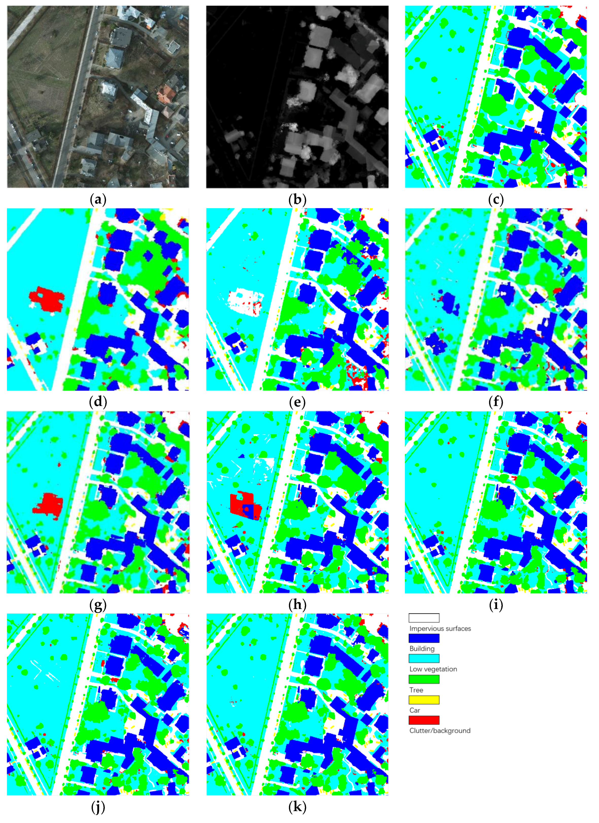
We further evaluate our model in the comparison to other classic or state-of-art networks, including FCN, DeepLab_v3, U-net and some methods on the leaderboard of ISPRS 2D datasets. SVL_1 is a traditional machine learning method based on Adaboost-based classifier and CRF. Though deep learning methods show an absolute advantage, it still can be a baseline method. DST_5 [48] employs a non-downsampling CNN that performs better than the original FCN. RIT6 [49] is a new approach published recently which uses two specific ways to extract features and fuses the feature maps at different stages.

Table 6. Quantitative result of different methods including FCN, DeepLab_v3, U-net, SVL_1, DST_5 and RIT6 on the Potsdam dataset.

Method	Precision	Recall	${\mathit{F}}_1$	OA
SVL_1	0.763	0.703	0.721	0.754
FCN [23]	0.807	0.823	0.812	0.824
DST_5 [48]	0.886	0.884	0.885	0.878
RIT6 [49]	0.886	0.892	0.888	0.879
U-net [27]	0.859	0.881	0.867	0.860
DeepLab_v3 [32]	0.881	0.886	0.882	0.878
DeepLab_v3+ [44]	0.882	0.889	0.884	0.880
Ours	0.885	0.893	0.888	0.883

shows the quantitative result of the methods mentioned above. As we can see, our proposed model has less misclassification areas as well as sharper object boundaries. The prediction results are shown in Figure 8.

4.3. The Influence of Superpixel-based DenseCRF

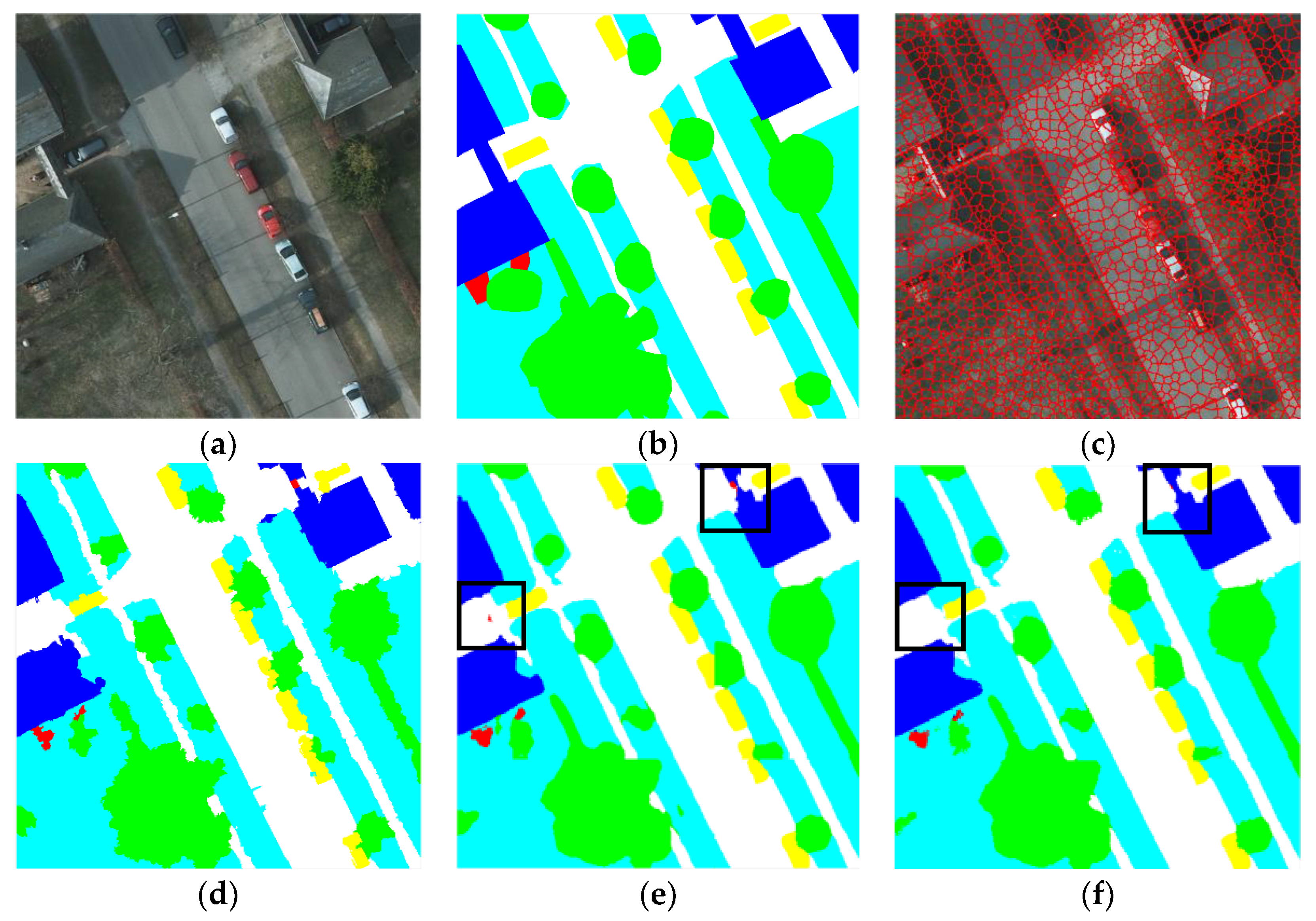
Dense Conditional Random Field (DenseCRF) is an effective postprocessing method to further refine the boundary of objects after FCN-based models. However, with the development of networks, the effect of enhancement has become weaker. In this study, we first apply classic DenseCRF after our model and the results show that the accuracy of prediction drops slightly. To improve the performance, inspired by the work of Zhao [50], we employ the superpixel algorithm (SLIC) before DenseCRF (details mentioned in Section 2.3). For overall accuracy, the superpixel-based DenseCRF brings 0.1% and 0.3% improvement on the Potsdam and the Vaihingen datasets respectively. Figure 9 and

Table 7. The comparison results before or after superpixel-based DenseCRF on the Potsdam and the Vaihingen datasets.

Potsdam	Precision	Recall	${\mathit{F}}_1$	OA
Before Superpixel-CRF	0.885	0.893	0.888	0.883
After Superpixel-CRF	0.888	0.892	0.889	0.884
Vaihingen	Precision	Recall	${\mathit{F}}_1$	OA
Before Superpixel-CRF	0.840	0.833	0.833	0.867
After Superpixel-CRF	0.847	0.833	0.835	0.870

show details. From the imageries, we can see that superpixel-based DenseCRF removes some small errors and the boundary of objects is slightly improved.

5. Conclusions

In this paper, a novel fully convolutional network to perform dense semantic labeling on high-resolution remote sensing imageries is proposed. The main contribution of this work consists of analyzing the advantage of existing FCN-based models, pointing out the encoder-decoder and ASPP as two powerful structures and fusing them in one model with an additional multi-scale loss function to take effect. Moreover, we employ several data augment methods before our model and a superpixel-based CRF as the postprocessing method. The objective of our work is to further improve the performance of fully convolutional network on dense semantic labeling tasks. Experiments were implemented on ISPRS 2D challenge which includes two high-resolution remote sensing imagery datasets of Potsdam and Vaihingen. Every object of the given categories was extracted successfully by our proposed method with fewer classification errors and sharper boundary. The comparison was taken between U-net, DeepLab_v3, DeepLab_v3+ and even some methods from the leaderboard including the recently published one. The results indicate that our methods outperformed other methods and achieved significant improvement.

Nowadays, remote sensing technology develops at a high-speed, especially the popularization of unmanned aerial vehicles and high-resolution sensors. More and more remote sensing imageries are available to be utilized. Meanwhile, deep learning based methods have achieved an acceptable result for practical applications. However, the groundtruth of remote sensing imageries are manually annotated and so will take too much labor. Therefore, semi-supervised or weak supervision methods should be taken into account in the future works.

References

- Moser, G.; Serpico, S.B.; Benediktsson, J.A. Land-cover mapping by Markov modeling of spatial-contextual information in very-high-resolution remote sensing images. Proc. IEEE 2013, 101, 631–651. [Google Scholar] [CrossRef]
- Xu, Y.; Wu, L.; Xie, Z.; Chen, Z. Building extraction in very high resolution remote sensing imagery using deep learning and guided filters. Remote Sens. 2018, 10, 144. [Google Scholar] [CrossRef]
- Xin, P.; Jian, Z. High-resolution remote sensing image classification method based on convolutional neural network and restricted conditional random field. Remote Sens. 2018, 10, 920. [Google Scholar]
- Marmanis, D.; Wegner, J.D.; Galliani, S.; Schindler, K.; Datcu, M. Semantic segmentation of aerial images with an ensemble of CNNs. ISPRS Ann. Photogramm. Remote Sens. Spat. Inf. Sci. 2016, 3, 473. [Google Scholar] [CrossRef]
- Li, M.; Zang, S.; Zhang, B.; Li, S.; Wu, C. A review of remote sensing image classification techniques: The role of spatio-contextual information. Eur. J. Remote Sens. 2014, 47, 389–411. [Google Scholar] [CrossRef]
- Kampffmeyer, M.; Arnt-Borre, S.; Robert, J. Semantic segmentation of small objects and modeling of uncertainty in urban remote sensing images using deep convolutional neural networks. In Proceedings of the IEEE Conference on Computer Vision and Pattern Recognition Workshops, Las Vegas, NV, USA, 26 June–1 July 2016; pp. 1–9. [Google Scholar]
- Michele, V.; Devis, T. Dense semantic labeling of subdecimeter resolution images with convolutional neural networks. IEEE Trans. Geosci. Remote Sens. 2017, 55, 881–893. [Google Scholar]
- Dalal, N.; Triggs, B. Histograms of oriented gradients for human detection. In Proceedings of the Computer IEEE Computer Society Conference on Vision and Pattern Recognition, San Diego, CA, USA, 20–25 June 2005; Volume 1, pp. 886–893. [Google Scholar]
- Lowe, D.G. Distinctive image features from scale-invariant keypoints. Int. J. Comput. Vis. 2004, 60, 90–110. [Google Scholar] [CrossRef]
- Herbert, B.; Andreas, E.; Tinne, T.; Luc, V.G. Speeded-up robust features (SURF). Comput. Vis. Image Underst. 2008, 110, 346–359. [Google Scholar]
- Inglada, J. Automatic recognition of man-made objects in high resolution optical remote sending images by SVM classification of geometric image features. ISPRS J. Photogramm. Remote Sens. 2007, 62, 236–248. [Google Scholar] [CrossRef]
- Mariana, B.; Lucian, D. Random forest in remote sensing: A review of applications and future directions. ISPRS J. Photogramm. Remote Sens. 2016, 114, 24–31. [Google Scholar]
- Turgay, C. Unsupervised change detection in satellite images using principal component analysis and k-means clustering. IEEE Geosci. Remote Sens. Lett. 2009, 3, 772–776. [Google Scholar] [CrossRef]
- Wang, H.; Wang, Y.; Zhang, Q.; Xiang, S.; Pan, C. Gated convolutional neural network for semantic segmentation in high-resolution images. Remote Sens. 2017, 9, 446. [Google Scholar] [CrossRef]
- Yansong, L.; Sankaranarayanan, P.; Sildomar, T.M.; Eli, S. Dense semantic labeling of very-high-resolution aerial imagery and LiDAR with fully-convolutional neural networks and higher-order CRFs. In Proceedings of the IEEE Conference on Computer Vision and Pattern Recognition (CVPR) Workshops, Honolulu, HI, USA, 21–26 July 2017; pp. 76–85. [Google Scholar]
- Hyeonwoo, N.; Seunghoon, H.; Bohyung, H. Learning Deconvolution Network for Semantic Segmentation. In Proceedings of the IEEE International Conference on Computer Vision, Washington, DC, USA, 3–7 December 2015; pp. 1520–1528. [Google Scholar]
- Krizhevsky, A.; Sutskever, I.; Hinton, G.E. Imagenet classification with deep convolutional neural networks. In Proceedings of the International Conference on Neural Information Processing Systems, Lake Tahoe, NV, USA, 3–6 December 2012; pp. 1097–1105. [Google Scholar]
- Deng, J.; Dong, W.; Socher, R.; Li, L.J.; Li, K.; Li, F.-F. ImageNet: A large-scale hierarchical image database. In Proceedings of the IEEE International Conference on Computer Vision and Pattern Recognition, Miami, FL, USA, 20–25 June 2009; pp. 248–255. [Google Scholar]
- Simonyan, K.; Zisserman, A. Very Deep Convolutional Networks for Large-Scale Image Recognition. arXiv, 2014; arXiv:1409.1556. [Google Scholar]
- He, K.; Zhang, X.; Ren, S.; Sun, J. Deep Residual Learning for Image Recognition. In Proceedings of the IEEE Conference on Computer Vision and Pattern Recognition (CVPR), Las Vegas, NV, USA, 26 June–1 July 2016; pp. 770–778. [Google Scholar]
- Huang, G.; Liu, Z.; Van Der Maaten, L.; Weinberger, K.Q. Densely connected convolutional networks. In Proceedings of the IEEE International Conference on Computer Vision and Pattern Recognition, Honolulu, HI, USA, 21–26 July 2017; pp. 4700–4708. [Google Scholar]
- Wei, X.; Fu, K.; Gao, X.; Yan, M.; Sun, X.; Chen, K.; Sun, H. Semantic pixel labelling in remote sensing images using a deep convolutional encoder-decoder model. Remote Sens. Lett. 2018, 9, 199–208. [Google Scholar] [CrossRef]
- Long, J.; Shelhamer, E.; Darrell, T. Fully convolutional networks for semantic segmentation. In Proceedings of the IEEE Conference on Computer Vision and Pattern Recognition, Boston, MA, USA, 7–12 June 2015; pp. 3431–3440. [Google Scholar]
- Fu, G.; Liu, C.; Zhou, R.; Sun, T.; Zhang, Q. Classification for High Resolution Remote Sensing Imagery Using a Fully Convolutional Network. Remote Sens. 2017, 9, 498. [Google Scholar] [CrossRef]
- Zhao, H.; Shi, J.; Qi, X.; Wang, X.; Jia, J. Pyramid scene parsing network. In Proceedings of the IEEE International Conference on Computer Vision and Pattern Recognition, Honolulu, HI, USA, 21–26 July 2017; pp. 2881–2890. [Google Scholar]
- Ronneberger, O.; Fischer, P.; Brox, T. U-net: Convolutional networks for biomedical image segmentation. In Proceedings of the International Conference on Medical Image Computing and Computer-Assisted Intervention, Munich, Germany, 5–9 October 2015; pp. 234–241. [Google Scholar]
- Chen, L.; Papandreou, G.; Kokkinos, I.; Murphy, K.; Yuille, A. DeepLab: Semantic image segmentation with deep convolutional nets, atrous convolution and fully connected crfs. IEEE Trans. Pattern Anal. Mach. Intell. 2017, 40, 834–848. [Google Scholar] [CrossRef] [PubMed]
- Peng, C.; Zhang, X.; Yu, G.; Luo, G.; Sun, J. Large kernel matters-improve semantic segmentation by global convolutional network. In Proceedings of the IEEE Conference on Computer Vision and Pattern Recognition, Honolulu, HI, USA, 21–26 July 2017; pp. 1743–1751. [Google Scholar]
- Chen, L.C.; Zhu, Y.; Papandreou, G.; Schroff, F.; Adam, H. Encoder-decoder with atrous separable convolution for semantic image segmentation. arXiv, 2018; arXiv:1802.02611. [Google Scholar]
- Szegedy, C.; Liu, W.; Jia, Y.; Sermanet, P.; Reed, S.; Anguelov, D.; Erhan, D.; Vanhoucke, V.; Rabinovich, A. Going deeper with convolutions. In Proceedings of the IEEE Conference on Computer Vision and Pattern Recognition, Boston, MA, USA, 8–10 June 2015; pp. 1–9. [Google Scholar]
- Maggiori, E.; Tarabalka, Y.; Charpiat, G.; Alliex, P. Fully convolutional networks for remote sensing image classification. In Proceedings of the IEEE International Conference on Geoscience and Remote Sensing Symposium (IGARSS), Beijing, China, 10–15 July 2016; pp. 5071–5074. [Google Scholar]
- Fisher, Y.; Vladlen, K. Multi-Scale Context Aggregation by Dilated Convolutions. arXiv, 2015; arXiv:1511.07122. [Google Scholar]
- Chen, L.C.; Papandreou, G.; Schroff, F.; Adam, H. Rethinking atrous convolution for semantic image segmentation. arXiv, 2017; arXiv:1706.05587. [Google Scholar]
- Shore, J.; Johnson, R. Properties of cross-entropy minimization. IEEE Trans. Inf. Theory 1987, 27, 472–482. [Google Scholar] [CrossRef]
- Bottou, L. Large-scale machine learning with stochastic gradient descent. In Proceedings of the 19th International Conference on Computational Statistics, Paris, France, 22–27 August 2010; pp. 177–186. [Google Scholar]
- Liu, F.Y.; Lin, G.S.; Shen, C.H. CRF learning with CNN features for image segmentation. Pattern Recognit. 2015, 48, 2988–2992. [Google Scholar] [CrossRef]
- Alam, F.I.; Zhou, J.; Liew, A.W.C.; Jia, X.P. CRF learning with CNN features for hyperspectral image segmentation. In Proceedings of the 2016 IEEE International Geoscience and Remote Sensing Symposium (IGARSS), Beijing, China, 10–15 July 2016; pp. 6890–6893. [Google Scholar]
- Wu, F. The potts model. Rev. Mod. Phys. 1982, 54, 235. [Google Scholar] [CrossRef]
- Achanta, R.; Shajji, A.; Smith, K.; Lucchi, A.; Fua, P.; Susstrunk, S. Slic superpixels compared to state-of-the-art superpixel methods. IEEE Trans. Pattern Anal. Math. Intell. 2012, 34, 2274–2281. [Google Scholar] [CrossRef] [PubMed]
- Van den Bergh, M.; Boix, X.; Roig, G.; de Capitani, B.; Van Gool, L. Seeds: Superpixels extracted via energy-driven sampling. In Proceedings of the 12th European Conference on Computer Vision-Volume Part VII, Florence, Italy, 7–13 October 2012; Springer: New York, NY, USA, 2012; pp. 13–26. [Google Scholar]
- Gerke, M. Use of the Stair Vision Library within the ISPRS 2D Semantic Labeling Benchmark (Vaihingen); Technical Report; University of Twente: Enschede, The Netherlands, 2015. [Google Scholar]
- Liu, Y.; Ren, Q.; Geng, J.; Ding, M.; Li, J. Efficient Patch-Wise Semantic Segmentation for Large-Scale Remote Sensing Images. Sensors 2018, 18, 3232. [Google Scholar] [CrossRef] [PubMed]
- Lin, M.; Chen, Q.; Yan, S. Network in network. arXiv, 2013; arXiv:1312.4400. [Google Scholar]
- Abadi, M.; Barham, P.; Chen, J.; Chen, Z.; Davis, A.; Dean, J.; Devin, M.; Ghemawat, S.; Irving, G.; Isard, M.; et al. Tensorflow: A system for large-scale machines learning. In Proceedings of the 12th USENIX Symposium on Operating Systems Design and Implementation, Savannan, GA, USA, 2–4 November 2016; pp. 265–283. [Google Scholar]
- Chen, L.C.; Papandreou, G.; Kokkinos, I.; Murphy, K.; Yuille, A.L. Semantic image segmentation with deep convolutional nets and fully connected crfs. arXiv, 2014; arXiv:1412.7062. [Google Scholar]
- Everingham, M.; Van Gool, L.; Williams, C.K.; Winn, J.; Zisserman, A. The pascal visual object classes (voc) challenge. Int. J. Comput. Vis. 2010, 88, 303–308. [Google Scholar] [CrossRef]
- Cordts, M.; Omran, M.; Ramos, S.; Rehfeld, T.; Enzweiler, M.; Benenson, R.; Franke, U.; Roth, S.; Schiele, B. The cityscapes dataset for semantic urban scene understanding. In Proceedings of the IEEE Conference on Computer Vision and Pattern Recognition, (CVPR), Las Vegas, NV, USA, 26 June–1 July 2016; pp. 3213–3223. [Google Scholar]
- Sherrah, J. Fully convolution networks for dense semantic labelling of high-resolution aerial imagery. arXiv, 2016; arXiv:1606.02585. [Google Scholar]
- Piramanayagam, S.; Saber, E.; Schwartzkopf, W.; Koehler, F. Supervised Classification of Multisensor Remotely Sensed Images Using a Deep Learning Framework. Remote Sens. 2018, 10, 1429. [Google Scholar] [CrossRef]
- Zhao, W.; Fu, Y.; Wei, X.; Wang, H. An Improved Image Semantic Segmentation Method Based on Superpixels and Conditional Random Fields. Appl. Sci. 2018, 8, 837. [Google Scholar] [CrossRef]
Figure 1.
Alternative network structures in dense semantic labeling (a) The classic FCN-32s, (b) The classic FCN-8s (with skip architecture), (c) Encoder-Decoder, (d) Atrous Spatial Pyramid Pooling and (e) Ours.
Figure 2.
The pipeline of our dense semantic labeling system, including data preprocessing, network training, testing and post-processing.
Figure 3.
The structure of ResNet50/101 which consists of one convolution layer and four Blocks. Each Block has several Bottleneck units. Inside the bottleneck unit, there is a shortcut connection between the input and output. In this study, we choose ResNet101 as the backbone of our model.
Figure 4.
The architecture of our proposed fully convolutional network with the fusion of ASPP and encoder-decoder structures. ResNet101 followed by ASPP is the encoder part to extract multiple scale contextual information. While the proposed decoder shown as the purple blocks refines the boundary of object. In the end, the multi-scale loss function guides the training procedure.
Figure 5.
A sample of remote sensing imagery with different channels of data and the corresponding groudtruth in the Potsdam datasets.
Figure 6.
A sample of the result of our proposed model on the Potsdam dataset. (a) the high-resolution remote sensing imageries. (b) the corresponding groundtruth. (c) the prediction maps of our proposed model.
Figure 7.
A sample of the result of our proposed model on the Vaihingen dataset. (a) the high-resolution remote sensing imageries (b) the corresponding groundtruth (c) the prediction maps of our proposed model.
Figure 8.
A sample of comparison prediction results of different methods on the Potsdam dataset. (a) input imagery, (b) normalized DSM, (c) corresponding ground truth, (d) result of SVL_1, (e) result of FCN, (f) result of DST_5, (g) result of RIT6, (h) result of U-net, (i) result of DeepLab_v3, (j) result of DeepLab_v3+ and (k) our model.
Figure 9.
The effect of superpixel based DenseCRF. Here we show a small patch of the original imagery from the Potsdam dataset (a) input imagery, (b) groundtruth, (c) superpixel segmentation to input imagery, (d) superpixel constraint to prediction map, (e) prediction map from our model and (f) prediction map after superpixel-based DenseCRF.