Deformable Faster R-CNN with Aggregating Multi-Layer Features for Partially Occluded Object Detection in Optical Remote Sensing Images

Abstract

The region-based convolutional networks have shown their remarkable ability for object detection in optical remote sensing images. However, the standard CNNs are inherently limited to model geometric transformations due to the fixed geometric structures in its building modules. To address this, we introduce a new module named deformable convolution that is integrated into the prevailing Faster R-CNN. By adding 2D offsets to the regular sampling grid in the standard convolution, it learns the augmenting spatial sampling locations in the modules from target tasks without additional supervision. In our work, a deformable Faster R-CNN is constructed by substituting the standard convolution layer with a deformable convolution layer in the last network stage. Besides, top-down and skip connections are adopted to produce a single high-level feature map of a fine resolution, on which the predictions are to be made. To make the model robust to occlusion, a simple yet effective data augmentation technique is proposed for training the convolutional neural network. Experimental results show that our deformable Faster R-CNN improves the mean average precision by a large margin on the SORSI and HRRS dataset.

1. Introduction

Recently, Convolutional Neural Networks (CNNs) [1] have achieved flourishing success for visual recognition tasks, such as image classification [2], semantic segmentation [3], and object detection [4]. With the powerful feature representation capability of Deep CNNs, object detection has witnessed a quantum leap in the performance on benchmark datasets. Within the last five years, there have been massive improvements on standard benchmarks such as PASCAL and COCO by the family of region-based CNNs. However, little effort has been made towards occluded object detection in optical remote sensing images. Besides, modeling geometric variations or transformations in the scale of objects, pose, viewpoint, and part deformations is a key challenge in optical remote sensing visual recognition.

Object detection in optical remote sensing images often suffers from several increasing challenges including the large variations in the visual appearance of objects caused by viewpoint variation, occlusion, resolution, background clutter, illumination, shadow, etc. In the past few decades, various methods have been developed for the detection of different types of objects in satellite and aerial images, such as buildings [5], storage tanks [6], vehicles [7], and airplanes [8]. In general, they can be divided into four main categories: Template matching-based methods, knowledge-based methods, OBIA-based methods, and machine learning-based methods. According to the selected template type, template matching-based methods could be further subdivided into two classes, as rigid template matching and deformable template matching [5,9]. For knowledge-based object detection methods, there are two kinds of the most widely used, which used prior knowledge involved geometric information and context information [10,11,12]. In general, OBIA-based object detection methods include two steps: Image segmentation and object classification [13]. With regard to machine learning-based methods, three crucial steps, which include feature extraction, feature fusion dimension reduction, and classifier training, play important roles in the performance of object detection. Many recent approaches have formulated object detection as feature extraction and classification problems and have achieved significant improvements.

With the prosperity and rapid development of CNNs, object detection tasks have been formulated as feature extraction and classification problems, whose results have been shown to be promising with the help of the powerful feature representation capability of advanced CNN architecture. Currently, the most popularly CNN-based object detection algorithms could be roughly divided into two streams: The region-based methods and the region-free methods. The region-based methods firstly generate about 2000 category-independent region proposals for the input image, extract a fixed-length feature vector from each proposal using a CNN, and then classify those regions and refine their spatial locations. As a ground-breaking work, R-CNN [4] consists of three modules. The first module generates category-independent region proposals that are fed into the second module. It is a large CNN to extract a fixed-length feature vector from each region, while the third module is a set of class-specific linear SVMs. Compared to traditional R-CNN and its accelerated version SPPnet [14], Fast R-CNN [15] trains networks using a multi-task loss in a single training stage, which simplifies learning and tremendously increases runtime efficiency. Merging the proposed RPN and Fast R-CNN into a single network by sharing their convolutional features, Faster R-CNN [16] enables a unified, deep-learning-based object detection system to run at near real-time frame rates. In contrast, the region-free methods frame object detection as a regression problem and directly estimates the objects region, which truly enables real-time detection. YOLO [17] is extremely fast because it utilizes a single convolutional network to simultaneously predict bounding boxes and class probabilities directly from full images in one evaluation. Using a single CNN as well, SSD [18] discretizes the output space of bounding boxes into a set of default boxes over different aspect ratios and scales per feature map location. Additionally, the network combines predictions from multiple feature maps with different resolutions to naturally handle objects of various sizes, which improves the accuracy on high-speed detection. What is noteworthy is that the above-mentioned CNN-based object detection algorithms are designed somewhat specially for general object detection benchmarks, which is not suitable for object detection in optical remote sensing images because the object instances occupy a minor portion of the image that usually have the characteristic of small size in the optical remote sensing images. Furthermore, to deal with the problem of small objects, some methods like Fast R-CNN and Faster R-CNN achieve this by directly up-sampling the input image at the training phase or testing phase. It significantly increases the memory usage and processing time.

However, CNNs are inherently limited to model geometric transformations shown in visual appearance. The limitations derive from the fixed geometric structures of CNN modules: A convolution operation samples the input feature map at fixed locations. As long as a standard CNN architecture is adopted, the only method available to model geometric transformations are artificially generating sufficient complete training samples with various deformations. As said by Cheng et al. [19], it is problematic to directly use it for object detection in optical remote sensing images because it is difficult to effectively handle the problem of object rotation variations. Rotation Invariant CNN (RICNN) augments training objects by rotating them 360 degrees by a step of 10 degrees, which does not actually solve the inherent limitation in CNN. The emergence of deformable convolution overcomes the mapping limitations in CNN [20]. By adding 2D offsets to the regular convolution grid in the standard convolution, deformable convolution sample features from flexible locations instead of fixed locations, allowing for the free deformation of the sampling grid. In other words, deformable convolution refines standard convolution by adding learned offsets. The deformable convolution modules can readily replace the convolution layer in standard CNN and form deformable ConvNet. The spatial sampling locations in deformable convolution modules are augmented with additional offsets, which are learned from data and driven by the target task. Deformable ConvNet is a simple, efficient, deep, and end-to-end solution to model dense spatial transformations. We believe that it is feasible and effective to learn dense spatial transformation in CNNs for object detection in optical remote sensing images.

In this paper, we present a deformable Faster R-CNN with aggregating multi-layer features for partially occluded object detection in optical remote sensing images. In other words, Deformable ConvNet, embedded within Faster R-CNN, is introduced in the field of optical remote sensing for object detection. The main contributions of this paper are summarized as follows:

➢

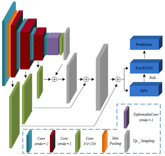
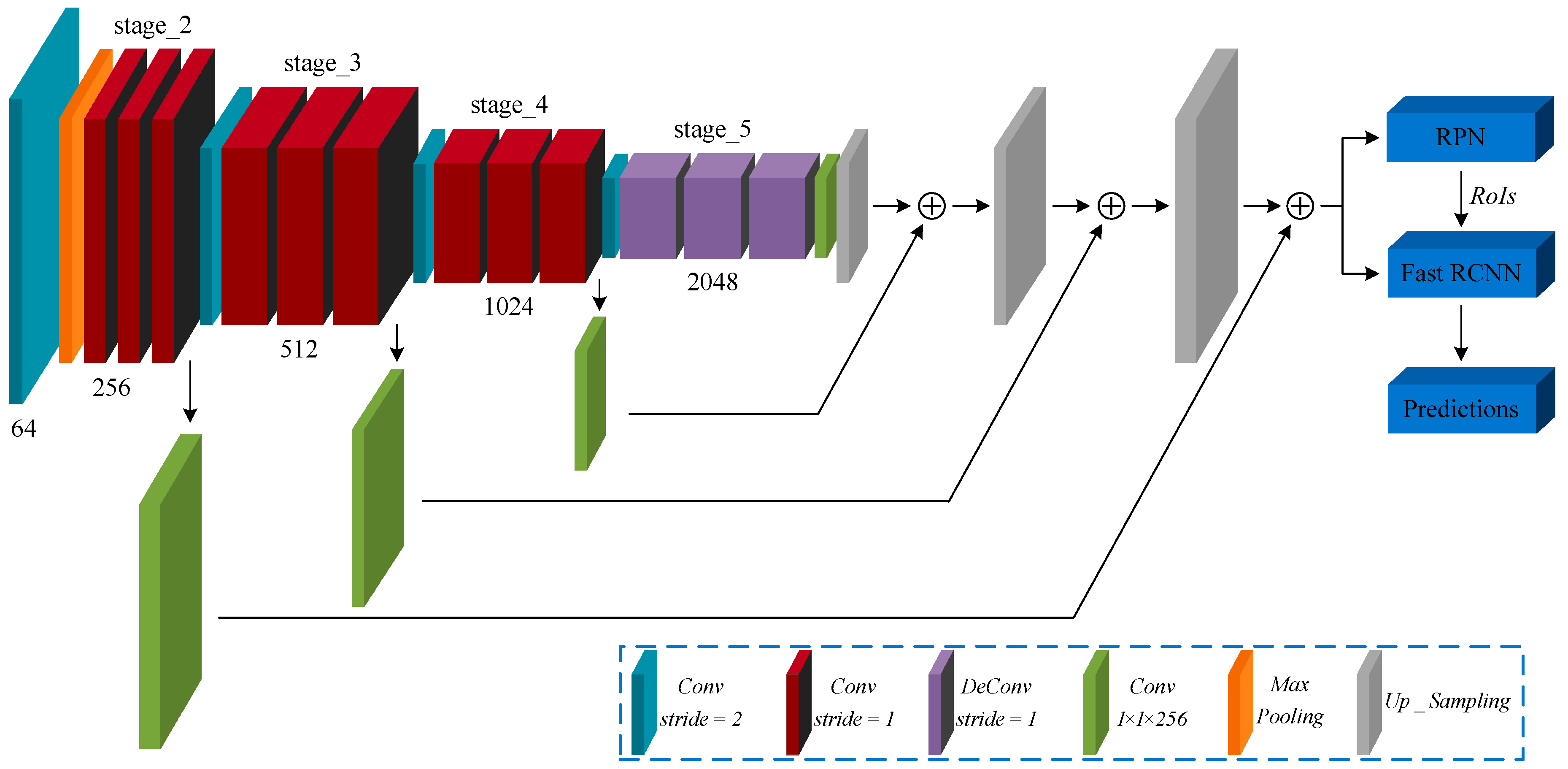
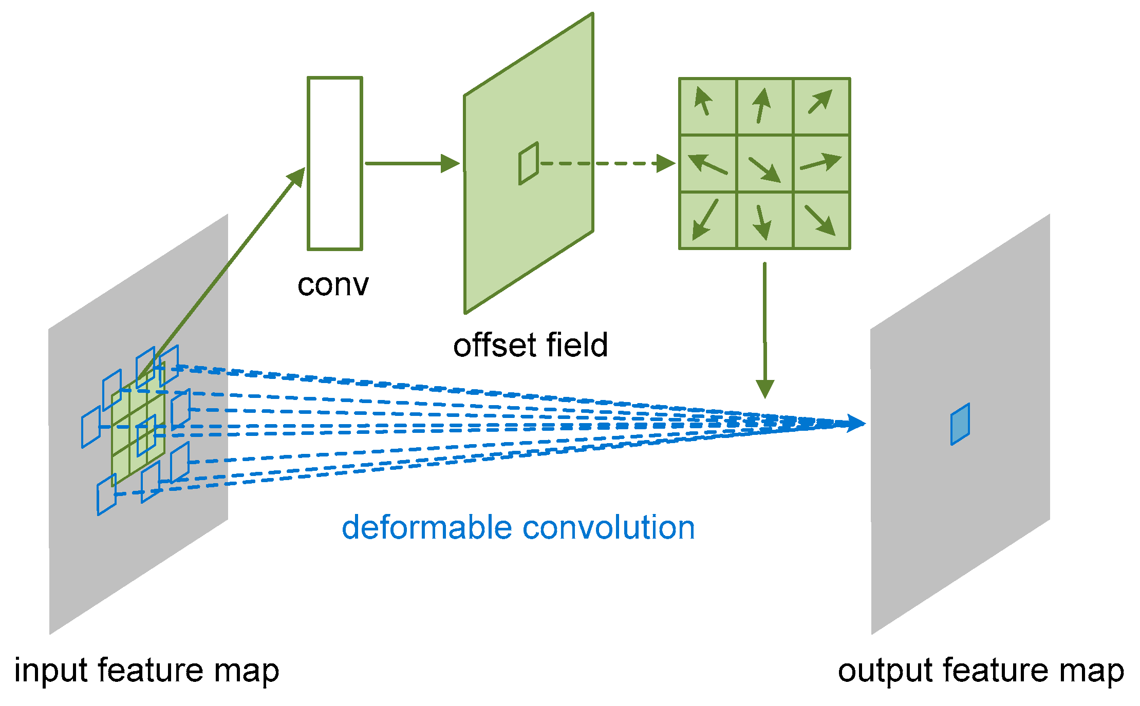
A unified deformable Faster R-CNN is introduced for object detection in optical remote sensing images. Geometric variation modeling is completed within the deformable convolution layers. Feature maps extracted by deformable ConvNet contain more information about various geometric transformations.

➢

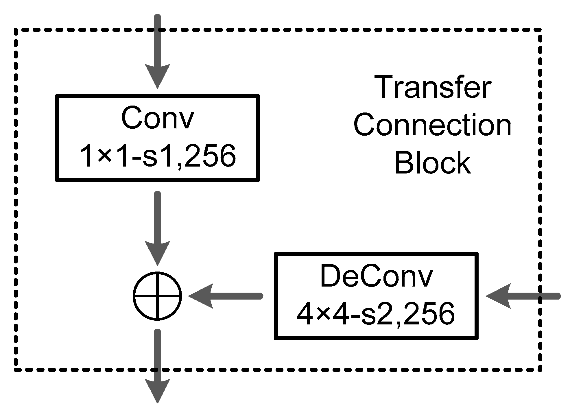
A modified backbone network is specially designed for small object to generate more abundant feature maps with high semantic information at low layer. Therefore, a Transfer Connection Block (TCB) adopting top-down and skip connections is presented to produce a single high-level feature map of a fine resolution.

➢

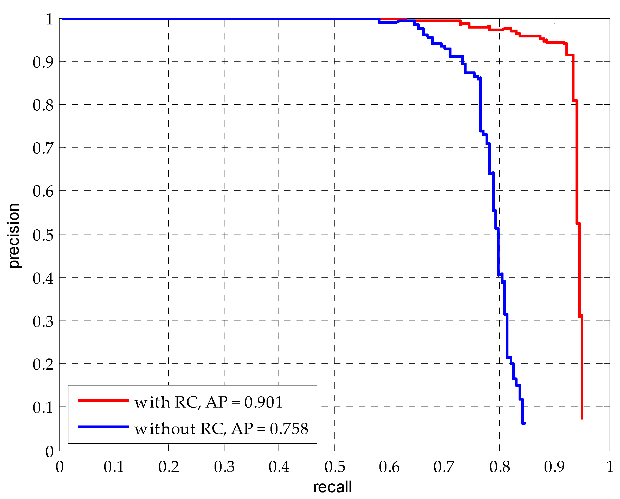
A simple, yet effective, data augmentation technique named Random Covering is proposed for training CNN. In training phase, it randomly selects a rectangle region in a region of interest and covers its pixels with random values. Hence, we can obtain augmented training samples with random levels of occlusion, which are fed into the model to enhance the generalization ability of the CNN model.

The rest of this paper is organized as follows. Section 2 introduces the methodology of our deformable Faster R-CNN with the transfer connection block. The last subsection of Section 2 proposes the data augmentation technique, namely the Random Covering. Section 3 presents the datasets and experimental settings. The results of our methodology and other approaches in the SORSI and HRRS dataset are presented in Section 4, while Section 5 gives our conclusion and the future work.

2. Methodology

Figure 1 presents a roundup of our deformable Faster R-CNN with three transfer connection blocks. Deformable Faster R-CNN is constructed by substituting the standard convolution layer with a deformable convolution layer in the fifth network stage. The proposed network consists of a deformable proposal network and a deformable object detection network, both of which share a deformable backbone network with three transfer connection blocks for feature map generation. More details are provided in the following content.

2.1. Deformable Convolution

While convolution in CNNs can be regarded as 3D spatial sampling, deformable convolution operates on the 2D spatial domain and remains the same across the channel dimension. In general, they are explained in 2D here. Extending the equations to 3D should be straightforward and omitted for notation clarity.

A standard 2D convolution consists of two steps: (1) Sampling using a regular grid $ℛ$ over the input feature map $X$; and (2) summation of sampled values weighted by $W$. The grid $ℛ$ defines the convolution kernel by size and dilation. For example, $ℛ$ = {(−1,1),(−1,0),…,(0,1),(1,1)} defines a 3 × 3 kernel with dilation 1. We can derive the standard convolution output of each position $p_0$ on the output feature map $Y$, according to the following formula:

$$Y\left(p_0\right)={\displaystyle \sum _{p_i\in \mathbf{ℛ}}W\left(p_i\right)\cdot X\left(p_0+p_i\right)}$$

(1)

In Dai et al. [20], deformable convolution was defined by augmenting the regular grid $ℛ$ with 2D offsets $\left\{\Delta p_i|i=1,\dots ,N\right\}$, where $N=\left|\mathbf{ℛ}\right|$. Then the deformable convolution output of each position $p_0$ on the output feature map $Y$ can be formulized as follows:

$$Y\left(p_0\right)={\displaystyle \sum _{p_i\in \mathbf{ℛ}}W\left(p_i\right)\cdot X\left(p_0+p_i+\Delta p_i\right)}$$

(2)

Obviously, the sampling is over the unfixed positions $p_i+\Delta p_i$ of the input feature grid. As the offset $\Delta p_i$ might be non-integer, Equation (2) is implemented by bilinear interpolation to obtain the fractional position. As we know, the bilinear interpolation can be formulated as

$$X\left(p\right)={\displaystyle \sum _{q}G\left(q,p\right)\cdot X\left(q\right)}$$

(3)

where $p$ denotes an arbitrarily fractional position ($p=p_0+p_i+\Delta p_i$ for Equation (2)), $q$ enumerates four integral spatial positions nearest to the position $p$, and $G\left(\cdot ,\cdot \right)$ indicates the bilinear interpolation kernel. Note that $G$ can be decomposed into two 1D kernels as

$$G=g\left(q_x,p_x\right)\cdot g\left(q_y,p_y\right)$$

(4)

where the 1D bilinear interpolation kernel is defined as $g\left(a,b\right)=max\left(0,1-\left|a-b\right|\right)$.

As illustrated in Figure 2, the additional offsets are learned by adding a standard convolutional layer branch whose convolution kernel is the same spatial resolution as the current convolutional layer. Additionally, the output offset fields have the same spatial resolution with the input feature map. The output channel dimension is set at $2N$ to encode $N$ 2D offset vectors. During training, both the convolutional kernels for producing the output features and for generating offsets can be learned. The gradients enforced on the deformable convolution layer can be back-propagated through the bilinear operations in Equations (3) and (4).

2.2. Transfer Connection Block

Generally, the objects have the characteristics of small size in the optical remote sensing images. The region-based methods consist of a region proposal network and an object detection network, both of which share a backbone network to generate feature representation. However, we notice that the feature maps of the shared network have a very large receptive field so that it can be hardly matched to small objects. The semantic information in the high-layer is significant for feature representation [21]. Based on these two considerations, the transfer connection block is presented to combine high semantic features from higher layers with fine details from lower layers, which is shown in Figure 3. To match the dimensions between them, the de-convolution operation is used to enlarge the high-level feature maps and sum them in the element-wise way. To be specific, the modified backbone network produces feature maps through three TCBs, starting from the last layer of the backbone network, which has high semantic information. Then the feature maps of the last layer are transmitted back to combine bottom-up feature maps at middle layers by top-down and skip connections. The TCP is sequentially embedded into the last three stages of the backbone network. By default, ResNet_50 is used to be the backbone network [22].

2.3. Random Covering

Occlusion caused by fog or cloud is a critical influencing factor on the generalization ability of CNNs in optical remote sensing images. It is desirable to achieve invariance to various levels of occlusion. When some parts of an object are occluded, a strong detection model should recognize its category and locate it from the overall object structure. However, the collected training samples usually reveal limited variance in occlusion. In an extreme case when no occlusion happens in all the training objects, the learned CNN model will work well on the testing images without occlusion. But it may fail to recognize objects with partial occlusion because of the limited generalization ability of the CNN model. While we can manually augment occluded images to the training data, this process is costly and the levels of occlusion can be limited.

To address the occlusion problem and improve the generalization ability of CNNs, Random Covering is introduced as a new data augmentation approach. This idea is inspired by another data augmentation approach named Random Erasing [23]. In the training phase, Random Covering happens with a certain probability. For an image $I$, within a mini-batch in the training phase, it is randomly chosen to undergo either Random Covering with probability $p$, or kept unchanged with probability $1-p$. Random Covering randomly selects a rectangle region $I_{rc}$ in the image and adds random values on these selected pixels. Assume the size of the image is $W\times H$ and its area is $S=W\times H$. We randomly initialize the area of the covering rectangle region to $S_{rc}$, where $S_{rc}/S$ is in the range specified by minimum $s_l$ and maximum $s_h$. The aspect ratio $r_{rc}$ of covering rectangle region is randomly initialized between $r_1$ and $r_2$. Then the size of covering region $I_{rc}$ is $H_{rc}=\sqrt{S_{rc}\times r_{rc}}$ and $W_{rc}=\sqrt{S_{rc}/r_{rc}}$. A point $p=\left(x_{rc},y_{rc}\right)$ in the image $I$ is randomly initialized as the center of the covering region $I_{rc}$, where the left-top location $p_{lu}$ and the right-bottom location $p_{rb}$ are $\left(max\left(1,x_{rc}-\frac{W_{rc}}{2}\right),max\left(1,y_{rc}-\frac{H_{rc}}{2}\right)\right)$ and $\left(min\left(W,x_{rc}+\frac{W_{rc}}{2}\right),min\left(H,y_{rc}+\frac{H_{rc}}{2}\right)\right)$. After selecting the covering region $I_{rc}$, each pixel in $I_{rc}$ is assigned to the weighted summation of the original pixel and a random value. The weight coefficient $\lambda$ is randomly initialized in a range specified by minimum ${\lambda }_1$ and maximum ${\lambda }_2$. The Random Covering procedure is shown in Algorithm 1. In the case of object detection, we select covering region in the bounding box of each object. If there are multiple objects in the image, Random Covering is applied on each object separately.

Algorithm 1: Random Covering Procedure

Input: Input image $I$;   Area of image $S=W\times H$;   Covering probability $p$;   Area ratio range $s_l$ and $s_h$;   Aspect ratio range $r_1$ and $r_2$;   Weight coefficient range ${\lambda }_1$ and ${\lambda }_2$; Output: Covering image $I^{*}$. Initialization: $p_1$$\leftarrow$$Rand\left(0,1\right)$. if $p_1\ge p$ then   $I^{*}$$\leftarrow$$I$;   return $I^{*}$. else   $S_{rc}$$\leftarrow$$Rand\left(s_l,s_h\right)\times S$;   $r_{rc}$$\leftarrow$$Rand\left(r_1,r_2\right)$;   $\lambda$$\leftarrow$$Rand\left({\lambda }_1,{\lambda }_2\right)$;   $H_{rc}\leftarrow \sqrt{S_{rc}\times r_{rc}}$, $W_{rc}\leftarrow \sqrt{S_{rc}/r_{rc}}$;   $x_{rc}\leftarrow Rand\left(1,W\right)$, $y_{rc}\leftarrow Rand\left(1,H\right)$;   $p_{lu}$$\leftarrow$$\left(max\left(1,x_{rc}-\frac{W_{rc}}{2}\right),max\left(1,y_{rc}-\frac{H_{rc}}{2}\right)\right)$;   $p_{rb}$$\leftarrow$$\left(min\left(W,x_{rc}+\frac{W_{rc}}{2}\right),min\left(H,y_{rc}+\frac{H_{rc}}{2}\right)\right)$;   $I_{rc}$$\leftarrow$$\left(p_{lu},p_{rb}\right)$;   $I\left(I_{rc}\right)$$\leftarrow$$\lambda \cdot Rand\left(0,1\right)+\left(1-\lambda \right)\cdot I\left(I^{*}\right)$;   $I^{*}$$\leftarrow$$I$;   return $I^{*}$. end

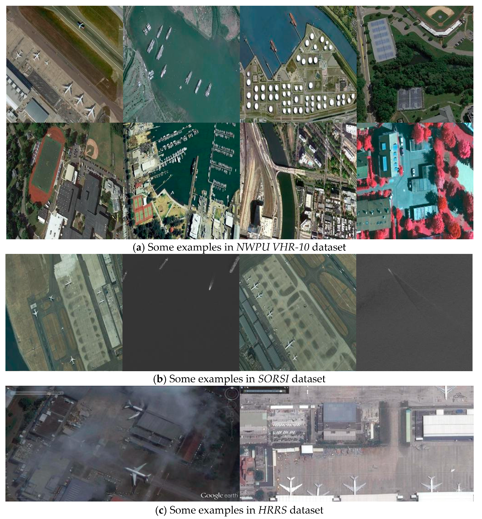
3. Dataset and Experimental Settings

To evaluate and validate the effectiveness of deformable Faster R-CNN on the optical remote sensing images, the datasets, experimental settings, and the corresponding evaluation metrics of the experimental results are described in this section.

3.1. Evaluation Metrics

Here, we explain two universally agreed and widely applied standard measures for evaluating the object detection methods, namely the Precision–Recall Curve (PRC) and Average Precision (AP). The first evaluation metric is based on the overlapping area between detections and ground truth. The Precision measures the fraction of detections that are true positives and the Recall measures the fraction of positives that are correctly identified. Let $TP$, $FP$, and $FN$ denote the number of true positives, the number of false positives, and the number of false negatives, respectively. The Precision and Recall can be formulated as:

$$Precision=\frac{TP}{TP+FP}$$

(5)

$$Recall=\frac{TP}{TP+FN}$$

(6)

In an object-level evaluation, detections are recognized as $TP$ if the area overlap ratio $\alpha$ between detections and ground truth object exceeds a predefined threshold $\lambda$ by the formula

$$\alpha =\frac{Area\left(detection\cap ground\_truth\right)}{Area\left(detection\cup ground\_truth\right)}>\lambda$$

(7)

where $Area\left(detection\cap ground\_truth\right)$ denotes the intersection of the detection and ground truth and $Area\left(detection\cup ground\_truth\right)$ denotes their union. Otherwise they are considered as $FP$. In addition, if several detections overlap with the same ground truth object, only one is considered as the true positive and the others are considered as false positives.

The second evaluation metric called AP is based on the area under the PRC. The AP computes the average value of Precision over the interval from $Recall=0$ to $Recall=1$. Mean AP (mAP) computes the average value of AP over all object categories. AP and mAP are used as the quantitative indicators in object detection. Typically, the higher the AP and mAP is, the better the detection performance, and vice versa.

3.2. Dataset and Implementation Details

To evaluate the performance of deformable Faster R-CNN, we conduct experiments on various optical remote sensing datasets. We chose three datasets, including the NWPU VHR-10 [24], SORSI [25], and HRRS [26] datasets. The NWPU VHR-10 dataset is a 10-class geospatial object detection dataset that contains a total of 650 annotated optical remote sensing images in the manner of VOC 2007. The ratios of training, validation and testing dataset are set to 20%, 20%, and 60%, respectively. Then, we randomly selected 130, 130, and 390 images to fill these three subsets, respectively. To make the model more robust to various input object sizes and shapes, each training image is sampled by the following options: (1) Using the original/flipped input image; and (2) rotating the input image by an angle step of 18°. The SORSI dataset contains only two categories: Ship and plane which includes 5922 optical remote sensing images—5216 images for ship and 706 images for plane. The numbers of this dataset in different classes are highly imbalanced, which poses great challenges for model training. To make a fair comparison, the SORSI dataset is randomly split into 80% for training, and 20% for testing as well. Some samples of these three datasets are shown in Figure 4. Besides, a more challenging occlusion dataset is collected by Qiu et al., which is available on https://github.com/ QiuWhu/Data. This dataset includes 47 images with total 184 airplanes, 105 airplanes of which are partially occluded by cloud or hangar or truncated by image border.

Adopting the alternating training strategy in this paper, we trained and tested both RPN and Fast R-CNN on images of a single scale based on Caffe [27] in all of the experiments. The images were resized such that their shorter side is 608 pixels under the premise of ensuring the longer side less than 1024 pixels. We used the pre-training model ResNet-50 to initialize the network. The deformable Faster R-CNN is constructed by substituting the standard convolution layer with a deformable convolution layer in the last three-network stage. For other newly added layers, we initialized the parameters by drawing weights from a zero-mean Gaussian distribution with standard deviation of 0.01. Furthermore, it is easy for our method to adopt Online Hard Example Mining (OHEM) [28] during training. Assuming $N$ proposals per image generated by RPN, in the forward pass, we evaluate the loss of all $N$ proposals. Then we sort all RoIs (positive and negative) by loss and select $B$ RoIs that have the highest loss. Back-propagation [29] is performed based on the selected proposals.

For the NWPU VHR-10 dataset, we trained a total of 80 K iterations, with a learning rate of 10⁻³ for the first 60 K iterations, 10⁻⁴ for the next 20 K iterations. The iteration was halved for the SORSI datasets. Weight decay and momentum were 0.0005 and 0.9, respectively. For anchors, we adopted three scales with box areas of 16², 40², and 100² pixels, and an aspect ratio of 1:1, which were adjusted for better coverage of the size distribution of our optical remote sensing dataset. At the RPN stage, we sampled a total of 256 anchors as a mini-batch for training (128 proposals for the Fast RCNN stage), where the ratio of positive to negative samples was 1:1. The evaluation metric is AP of each object and mAP with the Interception-of-Union (IoU) threshold set to 0.5. Non-Maximum Suppression (NMS) is adopted to reduce redundancy on the proposal regions based on their box-classification scores. The IoU threshold is fixed for NMS at 0.7. All experiments were performed on Intel i7-6700K CPU and NVIDIA GTX1080 GPU.

4. Experimental Results and Discussion

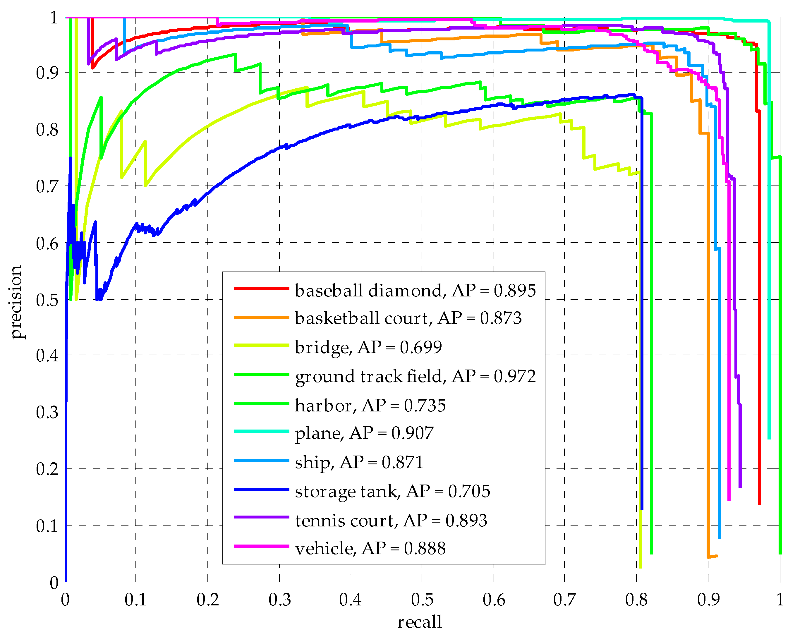
4.1. Quantitative Evaluation of NWPU VHR-10 Dataset

To evaluate the proposed deformable Faster RCNN with TCB quantitatively, we compared it with the AP values with four state-of-the-art CNN-based methods: (1) A rotation-invariant CNN (RICNN) model which considers rotation-invariant information with a rotation-invariant layer and other fine-tuned layers; (2) the SSD model with an input image size of 512 × 512 pixels; (3) the R-P-Faster RCNN [30] object detection framework; and (4) deformable R-FCN with the aspect ratio constrained NMS. The results of these methods all come out of the previous papers [31].

As shown in

Table 1. The AP values of the object detection methods on the NWPU VHR-10 dataset.

Method	RICNN	SSD	R-P-Faster R-CNN	Deformable R-FCN (ResNet-101) with arcNMS	Deformable Faster RCNN (ResNet-50) with TCB
Airplane	0.884	0.957	0.904	0.873	0.907
Ship	0.773	0.829	0.75	0.814	0.871
Storage tank	0.853	0.856	0.444	0.636	0.705
Baseball diamond	0.881	0.966	0.899	0.904	0.895
Tennis court	0.408	0.821	0.79	0.816	0.893
Basketball court	0.585	0.856	0.776	0.741	0.873
Ground track field	0.867	0.582	0.877	0.903	0.972
Harbor	0.686	0.548	0.791	0.753	0.735
Bridge	0.615	0.419	0.682	0.714	0.699
Vehicle	0.711	0.756	0.732	0.755	0.888
mean AP	0.726	0.759	0.765	0.791	0.844

, the proposed deformable Faster RCNN with TCB, which is fine-tuned on the ResNet-50 ImageNet pre-trained model, obtains the best mean AP value of 84.4% among all the object detection methods. It also indicates that our deformable faster RCNN with TCB achieves the best AP values for most classes, except baseball diamond, harbor, and bridge. In particular, the AP values of small objects like vehicle increase more than other objects, which illustrate the good performance of our methods for small object detection. This will be further verified through the results on the SORSI dataset in the next subsection. Compared with the second best method of deformable R-FCN with arcNMS, the AP values of seven objects are increased, including airplane (0.873 to 0.907), ship (0.814 to 0.871), storage tank (0.636 to 0.705), tennis court (0.816 to 0.893), basketball court (0.741 to 0.873), Ground track field (0.903 to 0.972), and Vehicle (0.755 to 0.888). Figure 5 plots the PRCs of our method over ten testing classes, respectively. The recall ratio evaluates the ability of detecting more targets, while the precision evaluates the quality of detecting correct objects rather than containing many false alarms. Obviously, the ground track field obtains the best performance, in comparison to other objects adopting the proposed method.

4.2. Quantitative Evaluation of SORSI Dataset

To verify the performance on detecting small objects in optical remote sensing images, we conduct experiments on the SORSI dataset, only including two categories: Plane and ship. Besides, the areas of bounding boxes falling in the ship category dominate from 10² to 50² pixels while those in the plane category possess from 50² to 100² pixels. In other words, the ship has smaller scale than the plane, which indicates that detecting ships is considerably more challenging. The results of the baseline come from [25]. From

Table 2. The results of modified Faster R-CNN on SORSI dataset.

Method	Baseline	Faster RCNN with TCB	Deformable Faster RCNN with TCB	Deformable Faster RCNN with TCB (+OHEM)
plane	0.729	0.778	0.792	0.862
Ship	0.850	0.826	0.831	0.903
mean AP	0.789	0.802	0.812	0.883

, it can be seen that the AP value for ship grows by five percentage points while adopting the TCB module, which manifests the TCB module, which is significant to detect smaller object. Besides, AP values for ship and plane steadily improves by one percentage point when deformable convolution layers are used. In addition, the final AP values for all objects have a big improvement while adding the OHEM mechanism in the training phase, especially for the ship category. This demonstrates that the TCB module works well with the OHEM mechanism for detecting small objects.

4.3. Quantitative Evaluation of HRRS Dataset

To verify the effectiveness of the proposed Random Covering on the partial occlusion problem, experiments are conducted on the HRRS dataset. This dataset only includes one category: Airplane. This dataset includes 47 images with total 184 airplanes, 105 airplanes of which are partially occluded by cloud or hangar or truncated by image border. Therefore, we only randomly cover the images, which contain one airplane at least. First, we conduct an experiment on the SORSI dataset. It is surprising that the AP value for plane gets improvement by 0.4 percentage points while the AP value for ship remains unchanged. This shows that the proposed Random Covering can work well on an un-occluded dataset and improve the generalization ability of our model. Second, all the images of the HRRS dataset are tested by the previous model. Figure 6 shows a comparison of PRC while the model trains with or without Random Covering. In addition, we count up the number of true positives for the partially occluded objects, as illustrated in the

Table 3. The AP and #TP on the HRRS dataset with or without RC.

Method	with RC	without RC
AP/#TP	0.901/96	0.758/77

. The results indicate that both the AP value and the TP increase by a large margin while adopting the Random Covering in the training phase.

5. Conclusions

In this paper, a unified deformable Faster R-CNN is introduced for modeling geometric variations in optical remote sensing images. Besides, we presented a transfer connection block aggregating multi-layer features to produce a single high-level feature map of a fine resolution, which is significant for detecting small objects. To improve the generalization ability of the CNN model and address the occlusion problem, we proposed a simple data augmentation approach named Random Covering, which was used in the training phase. Experiments conducted on three datasets show the effectiveness of our method. In the future work, we will focus on the balance between the TCB module and the average running time per image, and the effect of deformable convolution in the feature extraction network.

References

1. Lecun, Y.; Bengio, Y. Convolutional networks for images, speech, and time series. In Handbook of Brain Theory and Neural Networks; MIT Press: Cambridge, MA, USA, 1995. [Google Scholar]
2. Krizhevsky, A.; Sutskever, I.; Hinton, G.E. Imagenet classification with deep convolutional neural networks. In Proceedings of the Advances in Neural Information Processing Systems 2012, Lake Tahoe, NV, USA, 3–8 December 2012; pp. 1097–1105. [Google Scholar]
3. Long, J.; Shelhamer, E.; Darrell, T. Fully convolutional networks for semantic segmentation. In Proceedings of the IEEE Conference on Computer Vision and Pattern Recognition, Boston, MA, USA, 7–12 June 2015. [Google Scholar]
4. Girshick, R.; Donahue, J.; Darrell, T.; Malik, J. Rich feature hierarchies for accurate object detection and semantic segmentation. In Proceedings of the IEEE Conference on Computer Vision and Pattern Recognition, Columbus, OH, USA, 24–27 June 2014. [Google Scholar]
5. Stankov, K.; He, D.C. Detection of buildings in multispectral very high spatial resolution images using the percentage occupancy hit-or-miss transform. IEEE J. Sel. Top. Appl. Earth Obs. Remote Sens. 2014, 7, 4069–4080. [Google Scholar] [CrossRef]
6. Ok, A.O.; Başeski, E. Circular oil tank detection from panchromatic satellite images: A new automated approach. IEEE Geosci. Remote Sens. Lett. 2015, 12, 1347–1351. [Google Scholar] [CrossRef]
7. Wen, X.; Shao, L.; Fang, W.; Xue, Y. Efficient Feature Selection and Classification for Vehicle Detection. IEEE Trans. Circuits Syst. Video Technol. 2015, 25, 508–517. [Google Scholar] [Green Version]
8. An, Z.; Shi, Z.; Teng, X.; Yu, X.; Tang, W. An automated airplane detection system for large panchromatic image with high spatial resolution. Optik-Int. J. Light Electron Opt. 2014, 125, 2768–2775. [Google Scholar] [CrossRef]
9. Jain, A.K.; Ratha, N.K.; Lakshmanan, S. Object detection using Gabor filters. Pattern Recognit. 1997, 30, 295–309. [Google Scholar] [CrossRef]
10. Leninisha, S.; Vani, K. Water flow based geometric active deformable model for road network. ISPRS J. Photogramm. Remote Sens. 2015, 102, 140–147. [Google Scholar] [CrossRef]
11. Ok, A.O. Automated detection of buildings from single VHR multispectral images using shadow information and graph cuts. ISPRS J. Photogramm. Remote Sens. 2013, 86, 21–40. [Google Scholar] [CrossRef]
12. Ok, A.O.; Senaras, C.; Yuksel, B. Automated detection of arbitrarily shaped buildings in complex environments from monocular VHR optical satellite imagery. IEEE Trans. Geosci. Remote Sens. 2013, 51, 1701–1717. [Google Scholar] [CrossRef]
13. Blaschke, T.; Hay, G.J.; Kelly, M.; Lang, S.; Hofmann, P.; Addink, E.; Feitosa, R.Q.; Van der Meer, F.; Van der Werff, H.; Van Coillie, F.; et al. Geographic object-based image analysis—Towards a new paradigm. ISPRS J. Photogramm. Remote Sens. 2014, 87, 180–191. [Google Scholar] [CrossRef] [PubMed]
14. He, K.; Zhang, X.; Ren, S.; Sun, J. Spatial pyramid pooling in deep convolutional networks for visual recognition. In European Conference on Computer Vision; Springer: Cham, Switzerland, 2014. [Google Scholar]
15. Girshick, R. Fast R-CNN. In Proceedings of the 2015 IEEE International Conference on Computer Vision, Santiago, Chile, 7–13 December 2015. [Google Scholar]
16. Ren, S.; He, K.; Girshick, R.; Sun, J. Faster R-CNN: Towards real-time object detection with region proposal networks. In Proceedings of the Advances in Neural Information Processing Systems, Montreal, QC, Canada, 7–12 December 2015. [Google Scholar]
17. Redmon, J.; Divvala, S.; Girshick, R.; Farhadi, A. You only look once: Unified, real-time object detection. In Proceedings of the IEEE Conference on Computer Vision and Pattern Recognition, Las Vegas, NV, USA, 27–30 June 2016. [Google Scholar]
18. Liu, W.; Anguelov, D.; Erhan, D.; Szegedy, C.; Reed, S.; Fu, C.Y.; Berg, A.C. SSD: Single shot multibox detector. In European Conference on Computer Vision; Springer: Cham, Switzerland, 2016. [Google Scholar]
19. Cheng, G.; Zhou, P.; Han, J. Learning rotation-invariant convolutional neural networks for object detection in VHR optical remote sensing images. IEEE Trans. Geosci. Remote Sens. 2016, 54, 7405–7415. [Google Scholar] [CrossRef]
20. Dai, J.; Qi, H.; Xiong, Y.; Li, Y.; Zhang, G.; Hu, H.; Wei, Y. Deformable Convolutional Networks. 2017. Available online: http://openaccess.thecvf.com/content_ICCV_2017/papers/Dai_Deformable_Convolutional_Networks_ICCV_2017_paper.pdf (accessed on 22 August 2018).[Green Version]
21. Lin, T.Y.; Dollár, P.; Girshick, R.B.; He, K.; Hariharan, B.; Belongie, S.J. Feature Pyramid Networks for Object Detection. 2017. Available online: http://openaccess.thecvf.com/content_cvpr_2017/papers/Lin_Feature_Pyramid_Networks_CVPR_2017_paper.pdf (accessed on 22 August 2018).
22. Ren, Y.; Zhu, C.; Xiao, S. Object Detection Based on Fast/Faster RCNN Employing Fully Convolutional Architectures. Math. Probl. Eng. 2018, 2018, 3598316. [Google Scholar] [CrossRef]
23. Zhong, Z.; Zheng, L.; Kang, G.; Li, S.; Yang, Y. Random erasing data augmentation. arXiv, 2017; arXiv:1708.04896. [Google Scholar]
24. Cheng, G.; Han, J.A. A survey on object detection in optical remote sensing images. ISPRS J. Photogramm. Remote Sens. 2016, 117, 11–28. [Google Scholar] [CrossRef] [Green Version]
25. Ren, Y.; Zhu, C.; Xiao, S. Small Object Detection in Optical Remote Sensing Images via Modified Faster R-CNN. Appl. Sci. 2018, 8, 813. [Google Scholar] [CrossRef]
26. Qiu, S.; Wen, G.; Fan, Y. Occluded object detection in high-resolution remote sensing images using partial configuration object model. IEEE J. Sel. Top. Appl. Earth Obs. Remote Sens. 2017, 10, 1909–1925. [Google Scholar] [CrossRef]
27. Jia, Y.; Shelhamer, E.; Donahue, J.; Karayev, S.; Long, J.; Girshick, R.; Guadarrama, S.; Darrell, T. Caffe: Convolutional architecture for fast feature embedding. In Proceedings of the 22nd ACM International Conference on Multimedia, Orlando, FL, USA, 3–7 November 2014. [Google Scholar]
28. Shrivastava, A.; Gupta, A.; Girshick, R. Training region-based object detectors with online hard example mining. In Proceedings of the IEEE Conference on Computer Vision and Pattern Recognition, Las Vegas, NV, USA, 27–30 June 2016. [Google Scholar]
29. LeCun, Y.; Boser, B.; Denker, J.S.; Henderson, D.; Howard, R.E.; Hubbard, W.; Jackel, L.D. Backpropagation applied to handwritten zip code recognition. Neural Comput. 1989, 1, 541–551. [Google Scholar] [CrossRef]
30. Han, X.; Zhong, Y.; Zhang, L. An efficient and robust integrated geospatial object detection framework for high spatial resolution remote sensing imagery. Remote Sens. 2017, 9, 666. [Google Scholar] [CrossRef]
31. Xu, Z.; Xu, X.; Wang, L.; Yang, R.; Pu, F. Deformable ConvNet with Aspect Ratio Constrained NMS for Object Detection in Remote Sensing Imagery. Remote Sens. 2017, 9, 1312. [Google Scholar] [CrossRef]
Figure 1. Architecture of the deformable Faster CNN with three TCBs.
Remotesensing 10 01470 g001
Figure 2. Illustration of 3 × 3 deformable convolution.
Remotesensing 10 01470 g002
Figure 3. The overview of the transfer connection block.
Remotesensing 10 01470 g003
Figure 4. Example images of NWPU VHR-10/SORSI/HRRS datasets.
Remotesensing 10 01470 g004
Figure 5. Precision versus recall curve for the proposed method over the NWPU VHR-10 dataset.
Remotesensing 10 01470 g005
Figure 6. Precision versus recall curve for the HRRS dataset with/without RC.
Remotesensing 10 01470 g006