Abstract
Local authorities require information on shoreline change for land use decision making. Monitoring shoreline changes is useful for updating shoreline maps used in coastal planning and management. By analysing data over a period of time, where and how fast the coast has changed can be determined. Thereby, we can prevent any development in high risk areas. This study investigated the transferability of a fuzzy classification of shoreline changes and to upscale towards a larger area. Using six sub areas, three strategies were used: (i) Optimizing two FCM (fuzzy c-means) parameters based on the predominant land use/cover of the reference subset, (ii) adopting the class mean and number of classes resulting from the classification of reference subsets to perform FCM on target subsets, and (iii) estimating the optimal level of fuzziness of target subsets. This approach was applied to a series of images to identify shoreline positions in a section of the northern Central Java Province, Indonesia which experienced a severe change of shoreline position over three decades. The extent of shoreline changes was estimated by overlaying shoreline images. Shoreline positions were highlighted to infer the erosion and accretion area along the coast, and the shoreline changes were calculated. From the experimental results, we obtained (level of fuzziness) values in the range from 1.3 to 1.9 for the seven land use/cover classes that were analysed. Furthermore, for ten images used in this research, we obtained the optimal = 1.8. For a similar coastal characteristic, this value can be adopted and the relation between land use/cover and two FCM parameters can shorten the time required to optimise parameters. The proposed method for upscaling and transferring the classification method to a larger, or different, areas is promising showing (kappa) values > 0.80. The results also show an agreement of water membership values between the reference and target subsets indicated by > 0.82. Over the study period, the area exhibited both erosion and accretion. The erosion was indicated by changes into water and changes from non-water into shoreline were observed for approximately 78 km2. Accretion was due to changes into non-water and changes from water into shoreline for 19.5 km2. Erosion was severe in the eastern section of the study area, whereas the middle section gained land through reclamation activities. These erosion and accretion processes played an active role in the changes of the shoreline. We conclude that the method is applicable to the current study area. The relation between land use/cover classes and the value of FCM parameters produced in this study can be adopted.
1. Introduction
A shoreline represents the boundary where the land meets the sea. It does not form a permanent line, but is a dynamic environment, as the land and sea are changing in response to both natural and anthropogenic factors [1]. Natural factors include storms, waves, tides, and the rising of sea level constantly eroding and/or building up the shoreline. In addition, the shoreline can change due to disruption in littoral sediment transport processes, which supply sediment to the coastal system [1,2]. A lack of sediment within the system contributes to coastal erosion. Anthropogenic factors also play a strong role in shoreline change and include coastal development such as the development of industry, residence, aquaculture and the construction of jetties, seawalls, and dikes [3,4,5]. Shorelines can change over a wide range of different temporal and/or spatial scales [6]. They can change over periods ranging from hours to seasons—for example, due to waves, winds, tides and seasonal variations. Over a longer period, the changes may be caused by a shift in the natural sediment supply, and relative sea-level change [7]. This long term variations can only be observed after several years such as in decades to centuries and provide more predictable trends [8].
Various methods to determine shoreline changes are available in the literature, including (i) aerial photography, (ii) hydrodynamic, morphological data and beach profiles, (iii) Global Positioning System (GPS) surveys, (iv) Airborne Light Detection and Ranging (LiDAR), and (v) satellite imagery [9]. Previous methods to extract shorelines can be divided into two broad categories [10]. The first category comprises model-based methods which generated shoreline by intersecting a digital elevation model (DEM) with the water level at a desired tidal datum; for example shoreline mapping from LiDAR-based DEM and a ground survey [11,12]. The second category consisted of image-based methods, which extracted instantaneous shoreline data from images whose acquisition time was correlated with tidal data—for instance, shoreline mapping from digital photogrammetry [13] and remote sensing imagery [14]. Since remotely sensed images record a shoreline at a particular instant, modelling shoreline with remote sensing images should include estimation of its uncertainty [15,16]. The uncertainty in shoreline modelling can arise, due to an inherent variability in nature, such as variation of a shoreline over time and the presence of gradual transitions between land and water [17,18]. When a shoreline is clearly identified, however, the uncertainty in shoreline modelling can originate from errors during image processing and taking measurements [18]. Given that the shoreline is indistinct [19], it is best handled by soft classification [20]. Few studies exist on modelling shoreline using soft classification e.g., fuzzy c-means classification (FCM) and the linear spectral mixture model [21,22,23,24]. In a previous study, FCM classification was used to estimate the water memberships and then generate a shoreline margin by using a choice of thresholds [24]. To estimate membership values using FCM, the parameters as the number of classes, and as the level of fuzziness must be specified. The choice of these parameters is not always an easy task, especially when the user does not have any knowledge about the number of information classes. As an alternative, specific indices can be estimated to measure clustering performance with a range of cluster numbers and a range of fuzziness values. The transferability and the upscaling potential of the shoreline model to larger areas than those where it has been developed have only rarely been investigated. Better knowledge about the transferability and the upscaling potential would lead to the development of more robust shoreline models, which eventually would advance understanding of changes in the coastal environment.
In this study, we aim to test the transferability of the method developed in Dewi, et al. [24] to another area and to upscale it towards a larger area. Both transferability and upscaling were assessed by the optimization of the and parameters. The method was implemented on a series of images in the northern part of Central Java.
2. Study Area
The study was carried out in an area situated along the northern coast of Central Java Province, Indonesia. The central point is located at Geographic coordinates 6°53’42”S and 110°21’38”E. It is approximately 51 × 19 km in size. The study area is a deltaic plain formed by river sediment and has an elevation of less than 10 m above mean sea level (MSL). A higher elevation of more than 10 m is found at the south-western region of the SRTM (Shuttle Radar Topographic Mission) data as can be seen in Figure 1.
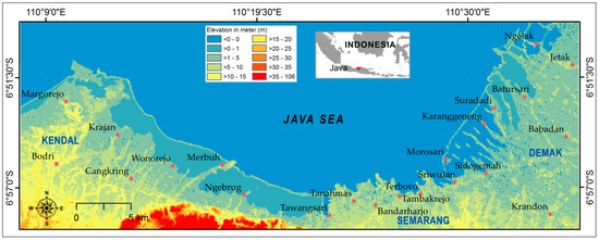
Figure 1.
A part of the northern coast of Central Java Province selected as the study site. It is visualized by the topographic data from Shuttle Radar Topographic Mission (SRTM) showing the topography of the area and village locations referred to in the text.
The area is categorized as a relatively low wave-energy coast and is influenced by the micro-tidal Java Sea [25]. In the Java Sea, the SWH (Significant Wave Height) in the wet season (December to February) ranges from 0.5 to 1.5 m with the highest SWH in February. In the dry season (June to August), the SWH ranges from 1 to 1.5 m with the highest SWH occurring in August and September [26]. Sofian and Wijanarto [26] mentioned that the maximum SWH was 3–3.5 m and 1–3 m during the wet and dry seasons, respectively. The dominant wave directions for the wet and dry seasons are eastward and westward, respectively. As waves approach and break along the coast, sediment moves alongshore in the direction of wave travel [27,28]. In this area, the general trend of sediment transport by longshore current moves from west and north-west to east [28,29].
Based on wind data from 2002–2012, Ervita and Marfai [30] stated that the prevailing wind during the wet season comes from west (32%) and north-west (31.7%), with a magnitude from 3.6 to 5.6 ms−1 (40.2%). In the dry season, the winds mostly blow from the east (62.6%) at the same dominant speed (56%) [30,31]. The wind is considered a causal factor in the development of this coastal area, as it triggers waves and currents. In addition, the current velocity is 0.02–0.04 ms−1 and 0.01–0.05 ms−1 for wet and dry seasons, respectively [32].
The study area covers a portion of the northern coastal area of three districts which include the cities of Demak on the east, Semarang in the middle and Kendal on the west with population sizes equal to 1118, 1700, and 942 inhabitants, respectively [33]. Reclamation activities in Semarang have a long history dating back to the 1980s [34]. Land reclamation started in 1979 to develop the Tanah Mas real estate, followed by Puri Anjasmoro in 1985, and Marina in 2004 [35]. In addition, the developments of the national harbour and airport, as well as the Terboyo industrial complex were also conducted through land reclamations in the 1980s and 1990s, respectively. Many of those reclamation activities are still ongoing.
The area is dominated by fishponds at the northern edge of the land. The Central Java Province is well known as one of the largest milkfish producers in Indonesia. Many rivers run across the areas and have been used for irrigation purposes for centuries, since the area is a paddy-dominated agricultural area. The rivers differ in size with discharges varying from 10 to 675 m3·s−1 in 2013 [36,37]. The rivers carry substantial quantities of sediment to the coast. As the coastal area has low wave energy, the sediment is deposited around the mouth of the rivers creating sand barriers (cheniers) at certain locations.
The area has a mixed semi-diurnal tide with two high tides and two low tides of varying heights. The average tidal range is 1.0 m [38]. In this area, tidal floods occur regularly in line with the tidal cycles. Therefore, Marfai [39] defined tidal floods as coastal flooding caused by high tide. In addition, Harwitasari and van Ast [40] mentioned that the impact of tidal floods in the study area (see Figure 2) was intensified by a combination of land subsidence and a rise in sea level [41,42]. Instead of periodic tidal floods, this area, especially Semarang city, faces local inundation caused by rainfall and river flooding, due to water overflow from the hinterland [43]. Sayung, located in the eastern part of Semarang city, has been threatened by massive erosion since 1998. In 2000 and 2007, hundreds of households from two villages were evacuated as coastal erosion destroyed houses [44,45].
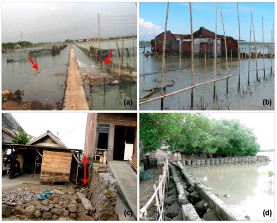
Figure 2.
Some impacts of coastal erosion, inundation and subsidence in the study area: (a) Eroded land alongside the elevated road (red arrows show the initial width of the road); (b) inundated houses; (c) a house with an elevated floor; and (d) embankment and mangrove for coastal protection.
3. Methodology
3.1. Satellite Images, Reference Data and Data Pre-Processing
Landsat and ASTER images with 30 m resolution available from USGS EarthExplorer [46] were used in this study (Table 1). In total, 10 images from 1988 to 2017 were used, denoted as , where is the image number . Seven images were recorded at the low tide with very small variation in water level, while the three images in 1994, 2000 and 2009 were recorded at high tide. Tidal data relating to the time of image acquisition were collected from the Indonesia Geospatial Information Agency [38].

Table 1.
Images used in this study and their related reference data.
All images were transformed to the Universal Transverse Mercator (UTM), World Geodetic System (WGS 84) projection. Landsat 8 OLI/TIRS images were rescaled to the same 8-bit format as Landsat TM, Landsat ETM+ and ASTER images. A histogram minimum adjustment was applied to all images [47] to reduce the effect of atmospheric path radiance. The Landsat 8 OLI/TIRS image from 19 June 2017 was rectified using a 2015 orthoimage. This Landsat image was then used as the base image to which all other images were geo-rectified using >70 ground control points (GCPs) of permanent features in the images. The images were then re-sampled to a 30 m pixel size using the nearest neighbour resampling method and the first order polynomial transform algorithm. The root mean square error (RMSE) was less than 0.5 pixels. Reference data from several images, including Sentinel-2, ASTER, Landsat TM [46] and images obtained via Google Earth were used for accuracy assessment purposes.
3.2. FCM Parameter Estimation for Land Use/Cover Types
Optimization of and parameters was performed for various land use/cover types in order to determine the relation between land use/cover composition and the value of and . For this purpose, the cluster validity index (CVI) was estimated based on Xie and Beni [48] by using a range of combinations of and . Values 1.1 to 3.0 were tested in the steps of 0.1 for . If equaled one, the FCM was a hard classifier, and an increase in tended to an increase in the level of fuzziness [49]. Pal and Bezdek [50] suggested the value of within the interval [1.5,2.5] as the best choice. In a previous study, = 1.7 produced the optimal result [24]. Values 2 to 7 were tested, in increments of one for , as there were seven land use/cover classes which were dominant in the area.
The CVI was used to evaluate the validity of partitions produced by the FCM clustering algorithm [50,51]. The lowest values produced by the CVI indicate a partition in which all the clusters are compact and separate from each other [48]. The CVI is estimated as:
where is the set of digital numbers; is the mean of the classes, is the number of pixels, is the number of classes, is the membership of pixel belonging to class , is the level of fuzziness, and is the minimum distance between the mean of the classes.
Small subsets consisting of approximately 30 × 30 pixels for seven land use/cover classes were created (i.e., water, fishpond, wet paddy, dry paddy, other crops, built-up, and bare soil) that could be identified in the study area. Subsets were collected over the full extent of images based on the dominant land use/cover of the subset area. To begin, a small number of subsets (i.e., 10 subsets) were used for each land cover class, and then the median value of and parameters were estimated. The number of subsets was then increased (i.e., 20, 30, 40, 50 subsets) to identify whether different median values for both parameters were obtained. When the difference between two median values was small (in the range of −0.1 to +0.1), the subsets were considered sufficient to describe the relation between land use/cover and the and values could be used for classification. In this case, increasing the number of subsets for the estimation may not achieve different results. Figure 3 shows the spatial distribution of the collected subsets for the cities of Semarang, Kendal and Demak.
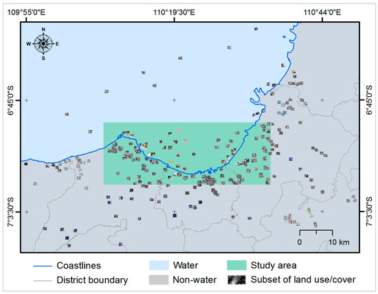
Figure 3.
Location of subsets for each land use/cover class in the cities of Semarang, Kendal and Demak.
3.3. Shoreline Model
The shoreline model, as developed in Dewi, et al. [24] was applied by performing FCM classification to derive shoreline margins by the choice of threshold interval (). To assess the transferability of the shoreline model and upscale towards a larger area, three strategies were used: (i) Optimizing and based on the predominant land use/cover of the reference subset by utilizing information provided in Section 3.2, (ii) adopting the values of and that resulted from the classification of the reference subset, to then perform FCM on the target subset, and (iii) estimating the optimal of the target subsets.
FCM classification was performed to estimate the membership value that separates the data cluster into sets so that each pixel has a membership value to multiple classes. The clustering used in the FCM was based on minimizing the within-groups sum of the squared error function [52]:
After choosing the number of classes , and the level of fuzziness , FCM adds an initial value to the of each class in order to initialise the clustering membership matrix. Instead of taking random values as the initial , the value of from the reference subset was used. The FCM classification was thus performed by iteratively estimating and updating the membership value and the mean cluster value [49,52]. After completing the clustering, membership images were compiled for each class. One of the membership images was labelled as belonging to the water class, using the infrared bands of the images. The water label was given to the class which had the minimum value of in the infrared bands [24]. The final and the optimal values were then evaluated by assuming that a large deviation of and from the reference subset indicated that a new choice of was required.
The possible shoreline location could then be determined by generating a margin or transition zone between the classes water and non-water. A threshold interval was defined based on kappa () estimation to create hard boundaries for the transition zone determined by the lower , and the upper thresholds. Threshold values from 0.1 to 0.9 were tested in steps of 0.05 to estimate the optimal threshold values and to generate a shoreline margin.
3.4. Subsetting
Subsets were crated for upscaling towards a larger area and to test the transferability to a different area. Subsets were denoted as , where is the subset number . Subset was selected as a reference subset. The reference subset was a subset whose parameters are used to initialise other subsets (target subsets). was considered at the corner of the study area (Figure 4a), thus obtaining a maximum distance between reference and target subsets for the purpose of upscaling. To upscale, three target subsets (subsets to , in Figure 4b–d) were created. The size was gradually increased to observe how various land use/cover influenced the values of and . In general, water was the dominant land use/cover in the area. To test the transferability of FCM to a different area, two more subsets (i.e., and ) were created of similar size to (see Figure 5). A detailed description of each subset is presented in Table 2.
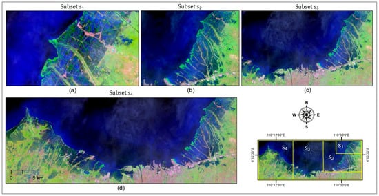
Figure 4.
Four subsets with various sizes were used to upscale the method to a larger study area. Subset (a) is a reference subset while the others are target subsets (b–d). False natural colour composite of 2017 Landsat image is used for visualisation. Dark blue represents water area, green refers to vegetation, and shades of pink refer to built-up.
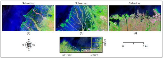
Figure 5.
Three subsets to test the transferability of the method to different areas. Subsets (a) and (b) are dominated by water and agriculture area while (c) is dominated by water and urban area.
Table 2.
The description of subsets used for upscaling and for testing transferability of the method.
The optimal FCM parameter was estimated at the reference subsets utilizing knowledge provided in Section 3.2. The values of c and were then estimated using the reference subsets for FCM classification of the target subsets. For upscaling, parameters of smaller subsets were applied to larger subsets. First, the optimal parameters for were estimated. Second, the value of and the same from classification were used to estimate . Likewise, the resulting class means of as the initial were used to estimate . Finally, the initial and values were compared with the final and the final values. For the transferability, the values of and were used from classification on the reference subset i.e., was used to estimate the target subsets and . To evaluate the performance, classifications on two different reference subsets were performed and compared. As a result, six shoreline images were produced, consisting of two reference subsets and four target subsets. The workflow implemented for the upscaling and transferability of the method is provided in Figure 6.
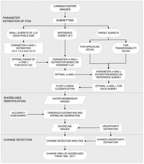
Figure 6.
Workflow implemented for upscaling and testing transferability of the method.
Each time the method was applied to either a larger area or another area with different land use/cover composition, the FCM updated the initial by considering the existing land use/cover composition. Large deviations in both and from their initial values indicated that the target subset required a new choice of for the FCM. Based on experiments conducted in this study, the deviations of and were acceptable if less than 15% and 20%, respectively. To check the variation of the infrared bands of the remote sensing images were used, because the bands exhibit a strong contrast between water and land features. The vegetation and soil show a high reflectance, but water shows low reflectance.
3.5. Analyzing Shoreline Changes
For the shoreline changes analysis, shoreline images developed for the whole study area (subsets ) were used. Post classification change detection was utilized by comparing information extracted from independently-produced classifications [53,54]. ‘From-to’ change information was provided, as well as the area and type of changes. Six types of changes were identified, namely shoreline to water, non-water to water, water to shoreline, non-water to shoreline, shoreline to non-water and water to non-water. These changes were identified as: (i) Abrupt changes when an area emerges at date without a corresponding area at date or vice versa, and (ii) gradual or partial changes when there is an expansion or shrinkage of areas that existed at both dates and .
Based on the results of shoreline change detection, the area of a specific change category was estimated by multiplying the number of pixels belonging to that specific change category by the area of a single pixel. Three sections of the coastal area were selected for analysing the change of shoreline margin at times and , namely east, middle and west sections. The first two sections experienced an extensive change of shoreline while the third section showed moderate shoreline change.
3.6. Change Uncertainty Estimation
By considering the vagueness of the shoreline position and the uncertainty inherent in image processing, the confidence of the changed area was then estimated. The area change was associated with a value that reflected the change certainty of the shorelines. In this study, the method proposed by Ardila, et al. [55] was modified, using differences in membership values estimated at and as proxy to the certainty in shoreline change. Six types of change certainties were identified namely change certainty of: Shoreline to water, non-water to water, water to shoreline, non-water to shoreline, shoreline to non-water and water to non-water. In addition to visualisation, each was regrouped into three types of change certainties namely change certainty to water, change certainty to shoreline and change certainty to non-water. For these change certainties, a high value corresponds to a high certainty of change in the shoreline image.
3.7. Accuracy Assessment
For accuracy assessment purposes, two error matrices were generated—conventional, and fuzzy. The conventional error matrix was used to assess the accuracy of shoreline models in the reference subset (), the accuracy of the transferability model ( and ) and the accuracy of the upscaling model (). For this purpose, a hardened FCM at the selected threshold = 0.5 was produced. We collected randomly 150 points (for , and ) and 400 points (for ) from each reference image. Subsequently, a visual interpretation approach was performed for a binary classification into water or non-water for each selected point. The kappa () values were then estimated by generating the confusion error matrix [56].
The fuzzy error matrix was developed to assess the agreement in water membership values between classes in the reference () and the target subsets when the method was upscaled to a larger area (, and ). For this purpose, 150 points were randomly collected from water membership images of both reference and target subsets. These points were collected over subset by assuming that the agreement obtained represented the accuracy of the classification for the entire target subset with respect to the reference subset. The fuzzy error matrix was obtained by finding the maximum possible overlap between the target and the reference subsets [57,58]. The overall accuracy of the classifications was then estimated.
4. Results
4.1. FCM Parameter and Threshold Values Estimation
From FCM parameter estimation on seven land use/cover types, we found that bare soil and wet paddy were found to have a similar optimal value of = 2 over the range between 2 and 7 for , while the value varied between 1.5 and 1.9. Water, fishpond, dry paddy and built-up obtained optimal values of between 2 and 3 with values ranging from 1.3 to 1.9. Other crops produced values between 1.5 and 1.7 and this class selects an optimal if lies between 2 and 6. Figure S1 shows histograms of the optimal and chosen by each CVI for seven land use/cover types in the study area. In this estimation, 55 subsets were used when the median values of and had very small variations. The complete results of the experiment can be seen in Table S1.
values were used to estimate an optimal threshold interval when generating the shoreline margin (see Figure 7). The highest values were given when values were between 0.3 and 0.7, though = 0.25 and = 0.75 also produced good results with values larger than 0.7 (except for ). It can be clearly seen that values lower than 0.25 and larger than 0.75 obtained an erratic curve. The selected threshold interval produced similar curves when κ values were estimated over time from 1988 up to 2017 (image up to ). Furthermore, before proceeding to generate shoreline margins for the whole images, the shoreline margins were visually evaluated by varying thresholds around the selected values. In this case, we set values 0.25 and 0.35 as and values 0.65 and 0.75 as . One threshold value was held constant (e.g., ) and the other threshold value () was varied to check whether extending the interval would give a large variation of margins. Changing and produced differences in the area of the shoreline margin. Based on the values and visual analysis when varying thresholds, the interval of 0.3 to 0.7 was chosen to generate the shoreline margins.
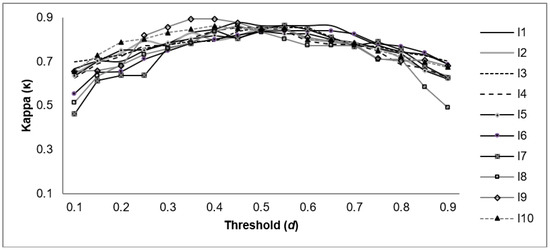
Figure 7.
values to estimate threshold interval for generating the shoreline margin. The curves show that values of larger than 0.7 and lower than 0.3 produced more erratic curves indicating low values. Threshold interval [0.3, 0.7] generally provides high values. Similar curves were obtained when estimated the for all images ( up to ).
4.2. Upscaling the Shoreline Model
Optimization of and was performed for as the reference subset for all images (see Figure S2a). FCM was applied by setting to 1.3–1.9, and to 2–3, based on information provided in Figure S1. For all these images, = 1.8 was obtained as the median value of the optimal and = 2 as the optimal chosen by each CVI.
The results of upscaling for and the related and values are presented in Figure 8. For this image, the reference and target subsets required similar and values ( = 1.8 and = 2). A complete optimization of target subsets is available in Figure S2b–d. In Figure 8, shoreline images are compared and zoomed in at red rectangle sites to show the detailed visualisation of the area (see Figure 8e–h). The shoreline margin of the target subset differed slightly (<2% of the area in the red rectangle sites) from its reference when upscaled. This was also supported by information provided in Figure 9. The class means of water decreased both in NIR (near infrared) and SWIR (shortwave infrared) bands. This may be related to the increase of water area especially clear water which has a low spectral reflectance value (see Figure 4). An increase of the class mean for non-water can be identified from subsets to . This may be due to the increase of built-up regions in both images as a result of city expansion. The small variation of shoreline margin (in Figure 8e–h) and the small shift in the value (in Figure 9) indicates that the differences (for e.g., land use/cover) between the smaller and the larger areas were small. However, we notice that the more we upscaled the method to a larger area, the larger the deviation of shoreline margin from subset denoted by an increase or decrease of the area (see Figure S3 and Table S2 for the complete results). This indicates the limitations of the upscaling method associated with the width of the image coverage used.
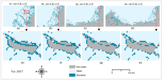
Figure 8.
Image is used to show the comparison of shoreline images developed at the reference subset (a) and the target subsets (b–d) by setting = 1.8 and = 2 as the optimal values for both parameters. We zoom into an area in the red rectangle site (e–h) to see a variation of shoreline margins (in turquoise) each time we upscaled the method to a larger area. The larger the area, the larger the deviation of shoreline margin from its reference subset.
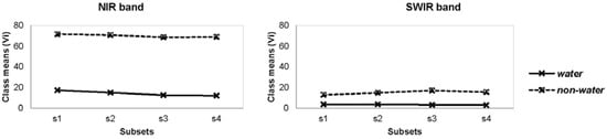
Figure 9.
The comparison of the resulting class means of subsets up to for image . The mean values of water class are slightly decreasing when we upscaled the method to larger areas both in NIR (near infrared) and SWIR (shortwave infrared) bands. Whereas, mean values of non-water class are decreasing in NIR band and increasing in SWIR band for subsets up to .
The method was upscaled towards larger areas for images , and . The overall accuracies were larger than 0.82 (see Table 3) for all subsets, showing a high agreement in water memberships between the reference subset and the target subsets. However, the overall accuracy slightly decreased with the increased area of the subsets. A complete accuracy assessment result can be seen in Table S3.
Table 3.
The overall accuracy indicating the water membership agreement between the reference subset and the target subsets ( up to ) estimated using fuzzy error matrix for images , and .
4.3. Transferability of the Method to Other Areas
The method was transferred to a different area with different land use/cover composition (see Figure 10). In Figure 10, was used as the reference subset and the resulting and values were used to estimate the two target subsets and . The reference and target subsets of image required similar and values ( = 1.8 and = 2). The complete optimization result of target subsets for other images is available in Figure S4.
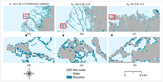
Figure 10.
Shoreline margin generated by transferring the shoreline model to target subsets for image . Subset (a) as the reference subset is used to estimate FCM (fuzzy c-means) parameter at target subsets (b,c). We zoom into an area in the red rectangle site (d–f) to see a variation of shoreline margin.
The comparison of the initial and final is provided in Figure 11. The mean of the water class increased from subset to in the NIR band, which was influenced by an increase of turbid water. The mean of the non-water class increased from subset to in the SWIR band, due to the increase of built-up areas.
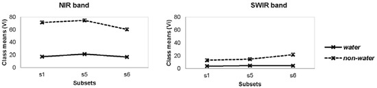
Figure 11.
The comparison of the initial and final when we transfer the method from subset to subsets and . FCM updates the initial considering the existing land use/cover of the area. The decrease of of water class in NIR band is related to the increase of clear water and the increase of of non-water class in SWIR band might be due to the increase of built-up area in subset .
As a comparison, Figure 12 shows the results of the shoreline images when was used as the reference subset to estimate FCM parameters of subsets and . We obtained different shoreline images compared to those in Figure 10. If the area of both results (subset in Figure 10 and Figure 12) were compared, the applied method overestimated the non-water area by 14% and the water area by 15.4% (see Figure 12e grid cells A2 and A3). There was also a large deviation in from its initial value (from 1.1 to 1.7) and a large shift of the non-water class mean, as seen in Figure 13, indicating that a new choice of was required when applying the method.
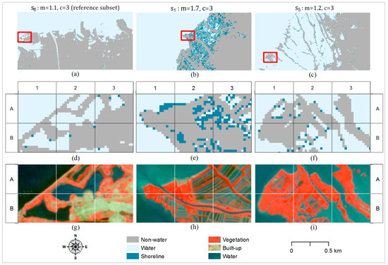
Figure 12.
Subset (a) is the reference subset to estimate the FCM parameter for subsets and (b,c). We zoom into the red rectangle sites to see a more detailed representation of the area (d–f). The 2017 Sentinel-2 images show the different types of land use/cover (g–i). The applied method clearly failed to identify the water area in subset (e,h) for e.g., grid cells A2, A3, and B2. It also failed to identify the shoreline margin in subset (f,i) near the vegetation areas for e.g., grid cells A1 and B1.
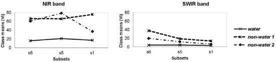
Figure 13.
The comparison of the initial and final when we transfer the method from subset to subsets and . There is a small variation of the water class means both in NIR and SWIR band from the reference subset to both target subsets. Meanwhile, there is a large variation of the non-water class specifically the non-water 2 in NIR band from subset to subset .
Thresholding at = 0.5 was performed to the six shoreline images provided in Figure 10 and Figure 12. The value of was 0.80 to 0.85, except for subset with a value of 0.51 (see Table 4). This low value reflects the low quality of the shoreline images produced using as the reference subset. Considering this low value, a large shift in from its initial value and the large deviation of shows that using subset to estimate subset was not be a good option. However, may be used to estimate considering a good value and low variations in the values of and .
Table 4.
The accuracy assessment results of shoreline images at threshold = 0.5 generated from two reference subsets ( and ).
4.4. Shoreline Change, Related Causes and Its Uncertainty
For the purpose of shoreline change analysis, ten shoreline images were used as a result of upscaling the shoreline model to the entire study area (see Figures S5–S7). Table 5 shows the values generated from a conventional error matrix when thresholding at = 0.5 was performed. We obtained values larger than 0.80.
Table 5.
The accuracy assessment results after thresholding at thresholds = 0.5 for the whole study area.
The spatial distribution of shoreline changes in the east section for each consecutive date is provided in Figure 14. Large changes into water were clearly seen for 1997–2000 and 2009–2013 and large changes in shoreline margin occurred for 2000–2003 and 2003–2006. These changes indicated an extensive erosion and inundation. In the past, this area was formed by deposition carried by rivers that drained into the Java Sea. However, an increase of population along with the development in the coastal area has disturbed this dynamic process. Moreover, land use/cover change in the upstream areas contributed to an increase in erosion and water discharge producing more sediment downstream. Not all of the sediment could be transported downstream. Small portions of the deposit were discharged into the sea, and others settled along the river bottom, irrigation canals and other water bodies. Therefore, this resulted in not only the narrowing and silting up of the canals and rivers, but also the reduction of the fluvial sediment supply into the coast [59].
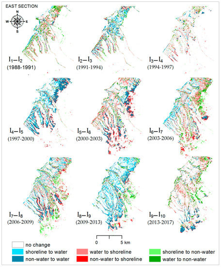
Figure 14.
The spatial distribution of shoreline changes in the east section of the study area for consecutive dates. The changed area was getting larger in the recent images from 2000, up to 2017, reflecting the severity of inundation in the area.
A massive land use/cover change in the adjacent area (Semarang city) contributed to the changes in shoreline in the east section as well. The port construction and massive land reclamation in the Semarang coastal area may have changed current directions, waves height and longshore sediment transport in the area [30]. The impact of coastal erosion destroyed fishponds (see Figure 15 boxes 2 and 4), settlements and agriculture areas (see Figure 15 boxes 1 and 3) from 1998. Images made available via Google Earth were used to visually classify the land use/cover affected by coastal erosion. Open water, fishponds, agricultural areas (paddy and other crops), mangroves, bare soil and settlements were distinguished. Dark green colours indicate vegetation (mangroves or agricultural area). Light green colours represent water areas (open water, river or fishponds), brown, light grey and white colours indicate settlements or residential areas and light brown colours indicate bare soil. Geometric patterns indicate fishponds and agricultural areas. While fishponds normally have a small and narrow pattern, agricultural areas have a wider pattern. There was a relation between coastal erosion contributing to the changes in shorelines with land use/cover (see Figure 15).
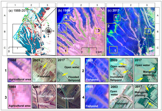
Figure 15.
Changes of land use/cover observed in the east section. (a) Spatial distribution of changes from 1988 to 2017. Black-dashed rectangle shows the locations of Landsat images with RGB 542 displayed in (b) and (c) corresponding to areas experiencing massive erosion. The pink colour represents bare soil, green refers to vegetation and blue refers to water. The four yellow boxes show zoom-in areas. The 1988 Landsat and Google Earth images show the type of land use/cover. Agricultural areas, fishponds, mangroves, open water, and settlements were distinguished based on criteria described in the text.
For the middle section (see Figure S8), a small increase in non-water areas occurred for 1988–1991 and 1994–1997, in particular in the west portion of the site, while a subtle change in water was shown for 1997–2000 and 2009–2013 in the east. The change in shoreline was indicated by coastal land reclamation from 1988 to 1991. In fact, the land reclamation began in the 1980s [34]. Coastal reclamation occurred on a large scale, due to the high demand for housing and economic activity (see Figure 16 boxes 1 and 2). Fishponds and marshes turned into urban areas including settlements, commercial and business areas, recreational areas and industrial zones, anticipating urban growth. Despite the fact that land reclamation expanded the space available for economic purposes, the activity came at a price, in terms of its negative impact on the environment. The construction of urban areas increased the surface runoff and reduced the ability of the ground to absorb rainfall. Furthermore, when there are major land use changes in coastal areas, fishponds, swamps and paddy fields turn into built-up areas. As a consequence, floods [34,35], land subsidence [60], and erosion [61] leading to coastal inundation occur not only in the urban zones that were developed on the marsh areas but also in adjacent areas (i.e., the east part of the middle section).
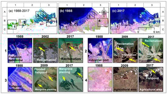
Figure 16.
Changes of land use/cover observed in the middle section. (a) Spatial distribution of changes from 1988 to 2017. Landsat images with RGB 542 from (b) 1988, and (c) 2017. Description of pixel colours can be seen in the caption of Figure 14. The four black boxes show zoomed-in areas. The 1988 Landsat and Google Earth images show the type of land use/cover. Agricultural areas, fishponds, mangroves, open water, and settlements were distinguished based on criteria described in the text.
Though substantial erosion and inundation occurred in the east and middle sections leading to a massive retreat of the shoreline position, a gradual accretion also leads to an advancing shoreline being identified. Replanting mangrove trees in response to coastal erosion was one of the causes of this accretion from the period 2003–2006 until 2013–2017 (see Figure 15 boxes 2 and 4 and Figure 16 box 3). An example of this was in Bedono [62] and Timbulsloko villages [63], in the middle section.
Compared to the east and middle sections, the west section (see Figure S9) showed a relatively constant condition, indicated by a small change in shoreline positions (of 8%) over three decades. A change in water occurred over the periods of 1997–2000 and 2009–2013, which indicated inundation (see Figure 17). Previous research mentioned that erosion and inundation changed the shoreline extensively and were also aggravated by land subsidence and the rising sea level [34,40,41,60]. The land subsidence is believed to be caused by the combination of natural consolidation of alluvium soil, ground water extraction and the load of buildings [42,43]. Ground water extraction occurs for industrial purposes and for the households’ needs, as the consequences of population growth. Excessive ground water extraction not only triggers land subsidence, but also salt water intrusion. Even though the inundation as a result of subsidence is much larger than that caused by sea level rise, a combination of land subsidence and sea level rise makes the shoreline more vulnerable to erosion by increasing wave height, in a muddy coastal environment [64]. Once erosion is initiated, the water and salinity levels start to rise in the remaining fishponds and further affect the agricultural area [65]. The inundated fishponds see a decline in fish productivity but it also leads to the abandonment of the fishpond area as mentioned by Wesenbeeck, et al. [64]. When fishponds are inundated, people revert to small-scale off-shore fishery practices [64]. Subsequently, if an agricultural area was inundated, and the farmers were no longer able to plant any crops, it was converted into a fishpond (see Figure 17 boxes 1 and 3). Only 6.8% non-water was gained over three decades, largely in the periods 1988–1991 and 2013–2017, due to land reclamation projects to develop the national airport, residential and business areas (see Figure 17 box 4).
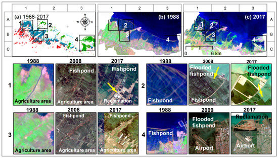
Figure 17.
Changes of land use/cover observed in the west section. (a) Spatial distribution of changes from 1988 to 2017. Landsat images with RGB 542 from (b) 1988 and (c) 2017. Description of pixel colours can be seen in the caption of Figure 15. The four black boxes show zoomed-in areas. The 1988 Landsat and Google Earth images show the type of land use/cover in those areas. Agricultural areas, fishponds, mangroves, open water, and settlements were distinguished based on criteria described in the text.
Overall change certainty of shoreline margin, water and non-water are presented in Figure 18. The change certainty is given for different levels of certainty within the black-dashed rectangle site. The area of each class changes with the change in the certainty level. The changed area for different levels of certainty for 1988 to 2017 can be seen in Table 6.
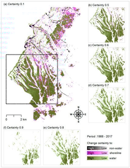
Figure 18.
(a) Change certainty of non-water, shoreline margin and water for the period 1988 up to 2017 in east section. (b–f) The change area is decreasing by the increase of certainty level.
Table 6.
Changed area (in number of pixels) between shoreline margin, water and non-water at different levels of certainty for the east section.
An example of shoreline change analysis, and its associated change certainty for 1988 to 2017 in the east section, is displayed in Figure 19. Changes from non-water to water (in turquoise) were related to high certainty of change into water (in dark green) as shown in Figure 19b,d, e.g., grid cells B2 and C2. This indicates the area which was inundated permanently. Changes from water to non-water (in dark green) were related to a high certainty of change into non-water (in black) and indicated by a reclamation area or the area where mangroves were planted as protection (see Figure 19b,d grid cells A1). Changes of non-water to shoreline (in dark red) with high certainty of change into shoreline (in dark purple) indicated an inundation influenced by tides (as in Figure 19b,d grid cells A3 and B3). In addition, changes of water to shoreline (in light red) with low certainty of change into shoreline (in light purple) might indicate sedimentation near mangrove areas (Figure 19b,d grid cell A1).
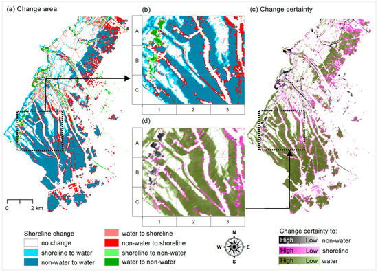
Figure 19.
Shoreline change (a,b) and its related change certainty (c,d) between 1988 and 2017. Large changes from non-water into water (turquoise) indicating a permanent inundation of the area are mostly related to the high certainty of change into water (dark green), whereas large changes of non-water into shoreline (red) might indicate the area which was inundated gradually.
Table 7 shows the overall changes of the three sections in 30 years. The largest shoreline changes occurred in the east section followed by the middle section: Both showing large changes from non-water to water for 22.7 and 17.9 km2, respectively. The second largest changes were the changes from non-water to shoreline which on the long term indicates a coastal inundation. This occurred for 8.5, 6.3 and 5.4 km2 in the east, west and middle sections, respectively.
Table 7.
Change area in km2 in the period 1988 up to 2017 with change certainty level ≥0.1. Changes to water indicate erosion and changes to non-water show accumulation. The coastal area in the east section experienced the largest loss of land in three decades.
5. Discussion
In this paper, the possibility of both transferability and upscaling of fuzzy classification were explored by adopting the method that we developed in Dewi, et al. [24]. To derive fuzzy shorelines, FCM was used to calculate the membership of water. To perform FCM, a suitable number of classes and level of fuzziness need to be specified either by users based on their a priori knowledge or estimated from images. This research provides information that can be used as the a priori knowledge to specify FCM parameters. The results revealed that there was a relation between land use/cover composition and the values of and . Seven land use/cover classes were analysed in this study and required values in the range of 1.3 to 1.9. Wet paddy and bare soil required = 2 as the optimal , whereas water, fishpond, dry paddy and built-up required = 2 to 3. The number of classes can vary up to six for other crops. When performing FCM for all images ( up to ) used in this study, = 1.8 was obtained as the median value of the optimal . This value is close to the value that we used in the previous study, where = 1.7 [24]. The range of values proposed by Pal and Bezdek [50] suggested an interval of [1.5–2.5] as the best choice for .
We proposed to use and values of the reference subset as the initial and values of the target subsets to upscale towards a larger area and to test the transferability of the method to another area with different land use/cover composition. The results show that the variation in spectral reflectance of the input image has a large influence on the number of classes needed for the FCM. The presence of water and moisture content on objects such as wet vegetation and wet soil decreases the reflectance in the infrared bands [66], therefore it requires a lower number of classes in FCM. On the contrary, dry vegetation, dry soil and concrete such as in urban area have a higher variation in spectral reflectance in the infrared bands. Therefore, they require a larger number of classes for the classification.
Adopting the same c value to transfer and upscale the model may cause a generalization of the classification that reduces the detail of land use/cover pattern of the initial data. Thereby, we might miss specific detailed, but relevant information. On the contrary, it is also possible that we set an unnecessary high number of classes that causes a longer time for parameter estimation yet a poor quality of shoreline images (see Figure 12e). As mentioned by Cihlar, et al. [67], a high number of clusters is not necessarily beneficial, since a smaller cluster may be meaningless.
In fact, for shoreline estimation, further detail in the non-water and water classes was not needed, though non-water and water show the largest spectral differences, especially in natural coastal areas with less urban structures, embankments or other coastal structures. Having only two classes in a coastal areas usually results in a split between water-related and land-related pixels. This assumption was adopted when using the water index to delineate water features [66] by enhancing features that have higher NIR reflectance and lower red light reflectance (e.g., vegetation). Those with low red light reflectance but very low NIR reflectance (e.g., water) will be suppressed. However, if the differences in area between sea and land are very large, having two classes may not be a good choice since the available classes will be distributed for e.g., in the land area. In this work, we evaluated the resulting of the target subsets. FCM updated the initial by considering the land use/cover condition of the target subset. The small differences in the resulting and indicated that the selected subsets differ little and tended to have a similar land use/cover. If there was a large shift in the two values, it indicates that the two subsets have large differences, and thus a new choice of value is required.
The proposed method was successful in performing FCM to estimate the water membership proven by high values larger than 0.80. However, due to limited availability of high resolution images, the conventional error matrix was constructed for accuracy assessment purposes after performing thresholding. In other situations, when high resolution images are available, soft reference data should be used to generate a fuzzy error matrix. Using a soft classifier to generate soft reference data is more likely to reduce the uncertainty, due to the vagueness of shoreline positions [58,68]. In addition, no information was lost, due to the hardening of the soft classification [69]. However, a thorough investigation is still required to estimate the FCM parameters of the higher resolution images.
The predominant land use/cover classes present in the area were considered when choosing FCM parameters, based on information provided in Section 4.1. The optimal values ( = 1.8) when performing FCM can be adopted, especially for similar coastal area characteristics which helps to shorten the time needed to optimize the parameters. However, the task remains difficult for the coastal area with a completely different characteristic—for example, a rocky cliff coast, a coast with sand and gravel, or a swampy coast with mangroves. An urban coastal area with more buildings, impervious surfaces and coastal structures requires a higher value because those features have a higher variation in spectral reflectance. Whereas, a natural coastal area with fewer hard structures requires a lower value since water bodies, wet soils and dark building roofs have a low spectral reflectance. For upscaling, gradually enlarging the area of target subsets results in small shifts in , thus FCM is able to keep up with the changes. However, there is a limitation to upscale towards a larger area if using the subsetting approach in this study (see Figure 4). The larger the area, the larger the shift of shoreline margin from its reference subset. Adopting a moving window may probably be an option to overcome this limitation [70]. FCM parameters could be updated using data inside a window centred on each location, and then the estimated parameters could be averaged using a moving window average. The parameters should then not abruptly vary between nearby locations, such that small deviations of and can be achieved.
In this study, we assessed shoreline changes and estimated change uncertainty for pixel locations. Two perspectives of changes were addressed: (i) The spectral and spatial uncertainty inherent to the shoreline in remote sensing images arising from spatial characteristics and vagueness, and (ii) the uncertainty in the changes propagating from the implementation of the developed change detection method. The first was addressed by applying a fuzzy classification to estimate the water membership, and the second by independent comparison of the changes with variation of water memberships for consecutive periods. An abrupt change produced strong variations of water memberships, while a gradual change produced smaller water membership differences.
Because shoreline position is one of the primary geo-indicators for environmental change [71], monitoring the changes of shoreline play an important role in achieving a balanced condition between development and environmental protection. Therefore, information on where and by how much the coastal area changed are important for coastal planners and government to prioritize activities. Furthermore, monitoring shorelines may contribute to making coastal cities safer and more resilient. By identifying areas that are more affected by the changes in shoreline, the government may adjust land use planning and move development away from prone areas.
6. Conclusions
This study investigates transferability of shoreline classification to other areas and upscaling to a larger study area. The experimental results concluded that: (i) and parameters can be optimized based on predominant land use/cover and the optimal value ( = 1.8) provided in this research can be adopted for similar coastal areas; and (ii) the value of and of the reference subset can be used to initialise target subsets. We conclude that the classification method in this study can be transferred to other areas and can be upscaled towards a larger study area.
The analysis of shorelines using the proposed method revealed a general trend of continuous shoreline changes as a result of erosion, inundation and accretion. Over the study period (1988–2017), erosion (indicated by the changes into water and shoreline) occurred over 78 km2. This area also experienced accretion (indicated by the changes into non-water and shoreline) over 19.5 km2. The extensive coastal erosion and inundation occurred mostly in the east section which brought damage to fishponds and agricultural areas. Massive shoreline changes occurred due to coastal land reclamation projects to install industrial and residential areas in Semarang City. However, to prove the influences of the reclamation activities to the severe shoreline changes is beyond the scope of this study.
Supplementary Materials
The following are available online at http://www.mdpi.com/2072-4292/10/9/1377/s1, Table S1: Median values of and parameters when increasing the number of subsets during parameter estimation, Figure S1: Histograms of optimal values of (left) and (right) obtained after performing cluster validity measures on seven land use/cover classes, Figure S2: Optimization results of value for FCM classification: (a) The optimal values of the reference subset () with = 2 as the optimal chosen by CVI for all images; (b–d) The optimal values as a result of upscaling towards larger areas by using as the reference subset and the optimal = 2 was obtained for all these target subsets, Figure S1: Image is used to show the comparison of shoreline images developed at the reference subset (a) and the target subsets (b–d). We zoom into four areas in the red rectangle sites (e–t) to see a variation of shoreline margins (in turquoise) each time we upscaled the method to a larger area, Table S2: The comparison of area ( up to ) for four selected sites in Figure S3 when upscaling towards larger area, Figure S4: The optimal values as a result of transferability to other areas by using as the reference subset, Table S3: The overall accuracy indicating water membership agreement between the reference () and target subsets ( up to ) estimated using the fuzzy error matrix, Figure S5: Shoreline images of the east section after upscaling towards a larger area (subset ), generated by setting threshold interval [0.3, 0.7], Figure S6: Shoreline images of the middle section, Figure S7: Shoreline images of the west section, Figure S8: The spatial distribution of shoreline changes in the middle section for consecutive dates, Figure S9: The spatial distribution of shoreline changes in the west section for consecutive dates.
Author Contributions
R.S.D. had responsibility for conducting the research including a writing task. W.B., A.S., and M.A.M. supervised the work, and revised the manuscript. All authors have read and approved the final manuscript.
Funding
This study was funded by the scholarship Program for Research and Innovation in Science and Technologies (RISET-PRO), Ministry of Research, Technology and Higher Education of Indonesia.
Acknowledgments
We thank V.A. Tolpekin and J.R. Bergado from Faculty of Geo-information Science and Earth Observation (ITC), University of Twente for providing the script code for FCM and cluster validity index. The constructive comments of reviewers on the earlier manuscript were gratefully appreciated.
Conflicts of Interest
The authors declare no conflict of interest. The funders had no role in the design of the study; in the collection, analyses, or interpretation of data; in the writing of the manuscript, and in the decision to publish the results.
References
- French, P.W. Coastal Defences: Processes, Problems and Solutions; Taylor and Francis: London, UK, 2001; p. 365. [Google Scholar]
- Dean, R.G.; Dalrymple, R.A. Coastal Processes: With Engineering Applications; Cambridge University Press: Cambridge, UK, 2002; p. 473. [Google Scholar]
- Wu, W.; Yang, Z.; Tian, B.; Huang, Y.; Zhou, Y.; Zhang, T. Impacts of coastal reclamation on wetlands: Loss, resilience, and sustainable management. Estuar. Coast. Shelf Sci. 2018, 210, 153–161. [Google Scholar] [CrossRef]
- Stefano, A.D.; Pietro, R.D.; Monaco, C.; Zanini, A. Anthropogenic influence on coastal evolution: A case history from the Catania Gulf shoreline (eastern Sicily, Italy). Ocean Coast. Manag. 2013, 80, 133–148. [Google Scholar] [CrossRef]
- Bergillos, R.J.; Rodrıguez-Delgado, C.; Millares, A.; Ortega-Sanchez, M.; Losada, M.A. Impact of river regulation on a Mediterranean delta: Assessment of managed versus unmanaged scenarios. Water Resour. Res. 2016, 52, 5132–5148. [Google Scholar] [CrossRef]
- Stive, M.J.F.; Aarninkhof, S.G.J.; Hamm, L.; Hanson, H.; Larson, M.; Wijnberg, K.M.; Nicholls, R.J.; Capobianco, M. Variability of shore and shoreline evolution. Coast. Eng. 2002, 47, 211–235. [Google Scholar] [CrossRef]
- Xu, N. Detecting Coastline Change with All Available Landsat Data over 1986–2015: A Case Study for the State of Texas, USA. Atmosphere 2018, 9, 107. [Google Scholar] [CrossRef]
- Dolan, R.; Fenster, M.S.; Holme, S.J. Temporal analysis of shoreline recession and accretion. J. Coast. Res. 1991, 7, 723–744. [Google Scholar]
- Gopikrishna, B.; Deo, M.C. Changes in the shoreline at Paradip Port, India in response to climate change. Geomorphology 2018, 303, 243–255. [Google Scholar] [CrossRef]
- Sukcharoenpong, A.; Yilmaz, A.; Li, R. An Integrated Active Contour Approach to Shoreline Mapping Using HSI and DEM. IEEE Trans. Geosci. Remote Sens. 2016, 54, 1586–1597. [Google Scholar] [CrossRef]
- White, S.A.; Parrish, C.E.; Calder, B.R.; Pe’eri, S.; Rzhanov, Y. LIDAR-Derived National Shoreline: Empirical and Stochastic Uncertainty Analyses. J. Coast. Res. 2011, 62, 62–74. [Google Scholar] [CrossRef]
- Kim, H.; Lee, S.B.; Min, K.S. Shoreline Change Analysis using Airborne LiDAR Bathymetry for Coastal Monitoring. J. Coast. Res. 2017, 79, 269–273. [Google Scholar] [CrossRef]
- Yao, F.; Parrish, C.E.; Pe’eri, S.; Calder, B.R.; Rzhanov, Y. Modeling Uncertainty in Photogrammetry-Derived National Shoreline. Mar. Geod. 2015, 38, 128–145. [Google Scholar] [CrossRef]
- Choung, Y.-J.; Jo, M.-H. Shoreline change assessment for various types of coasts using multi-temporal Landsat imagery of the east coast of South Korea. Remote Sens. Lett. 2016, 7, 91–100. [Google Scholar] [CrossRef]
- Dewi, R.S.; Bijker, W.; Stein, A. Comparing Fuzzy Sets and Random Sets to Model the Uncertainty of Fuzzy Shorelines. Remote Sens. 2017, 9, 885. [Google Scholar] [CrossRef]
- Zhao, X.; Stein, A.; Chen, X.; Zhang, X. Quantification of Extensional Uncertainty of Segmented Image Objects by Random Sets. IEEE Trans. Geosci. Remote Sens. 2011, 49, 2548–2557. [Google Scholar] [CrossRef]
- Riesch, H. Levels of Uncertainty. In Essentials of Risk Theory; Roeser, S., Hillerbrand, R., Sandin, P., Peterson, M., Eds.; Springer: Dordrecht, The Netherlands, 2013. [Google Scholar]
- Fisher, P.F. Models of uncertainty in spatial data. Geogr. Inf. Syst. 1999, 1, 191–205. [Google Scholar]
- Atkinson, P.M.; Foody, G.M. Uncertainty in remote sensing and GIS: Fundamentals. In Uncertainty in Remote Sensing and GIS; Foody, G.M., Atkinson, P.M., Eds.; John Wiley & Sons Ltd.: Hoboken, NJ, USA, 2002; pp. 1–18. [Google Scholar]
- Foody, G. Approaches for the production and evaluation of fuzzy land cover classifications from remotely-sensed data. Int. J. Remote Sens. 1996, 17, 1317–1340. [Google Scholar] [CrossRef]
- Muslim, A.M.; Foody, G.M.; Atkinson, P.M. Localized soft classification for super-resolution mapping of the shoreline. Int. J. Remote Sens. 2006, 27, 2271–2285. [Google Scholar] [CrossRef]
- Taha, L.G.E.-D.; Elbeih, S.F. Investigation of fusion of SAR and Landsat data for shoreline super resolution mapping: The Northeastern Mediterranean sea coast in Egypt. Appl. Geomat. 2010, 2, 177–186. [Google Scholar] [CrossRef]
- Huang, C.; Chen, Y.; Zhang, S.; Li, L.; Shi, K.; Liu, R. Spatial Downscaling of Suomi NPP–VIIRS Image for Lake Mapping. Water 2017, 9, 834. [Google Scholar] [CrossRef]
- Dewi, R.S.; Bijker, W.; Stein, A.; Marfai, M.A. Fuzzy Classification for Shoreline Change Monitoring in a Part of the Northern Coastal Area of Java, Indonesia. Remote Sens. 2016, 8, 190. [Google Scholar] [CrossRef]
- Ongkosongo, O. Indonesia. In Encyclopedia of the World’s Coastal Landforms; Bird, E.C.F., Ed.; Springer: Dordrecht, The Netherlands, 2010; Volume 1. [Google Scholar]
- Sofian, I.; Wijanarto, A.B. Simulation of Significant Wave Height Climatology using WaveWatehm. Int. J. Geoinf. 2010, 6, 13–19. [Google Scholar]
- Sulaiman, D.M. Proposed Coastal Erosion Management for the Northern Coast of Java Indonesia; Oregon State University: Corvallis, OR, USA, 1989. [Google Scholar]
- Hendriyono, W.; Wibowo, M.; Hakim, B.A.; Istiyanto, D.C. Modeling of Sediment Transport Affecting the Coastline Changes due to Infrastructures in Batang—Central Java. In Proceedings of the 2nd International Seminar on Ocean and Coastal Engineering, Environment and Natural Disaster Management (ISOCEEN), Surabaya, Indonesia, 13 December 2016; pp. 166–178. [Google Scholar]
- Putri, R.W.B.; Atmodjo, W.; Sugianto, D.N. Longshore current dan pengaruhnya terhadap transport sediment di perairan pantai Sendang Sikucing, Kendal. J. Oseanogr. 2014, 3, 635–641. [Google Scholar]
- Ervita, K.; Marfai, M.A. Shoreline Change Analysis in Demak, Indonesia. J. Environ. Prot. 2017, 8, 940–955. [Google Scholar] [CrossRef]
- Fitrianti, N.; Haryanto, Y.D.; Simamora, E.V.S.; Bintari, H.F.A.; Hartoko, A.; Anggoro, S.; Zainuri, M. Analysis of daily wind circulation toward sea level rise in Semarang. In Proceedings of the Maritime Sciences and Advanced Technology (MSAT), Denpasar, Bali, 3–5 August 2017. [Google Scholar]
- BIG. Ina-COAP. Available online: http://tides.big.go.id/las/UI.vm (accessed on 8 August 2018).
- BPS. Population and Population Growth Rate by Regency/Municipality in Jawa Tengah Province, 2010, 2014, and 2015. Available online: https://jateng.bps.go.id/linkTabelStatis/view/id/1353 (accessed on 23 October 2017).
- Miladan, N. Communities’ Contributions to Urban Resilience Process: A Case Study of Semarang City (Indonesia) Toward Coastal Hydrological Risk; Universit le Paris-Est: Paris, France, 2016. [Google Scholar]
- Pratiwi, M.R.I. Impact of the Tidal Floods Dynamics to Social Ecological System of Semarang City (Case Study in Tanjung Mas District). Master’s Thesis, Institut Pertanian Bogor, Bogor, Indonesia, 2012. [Google Scholar]
- Murtiaji, C.; Wibowo, M.; Irfani, M.; Hakim, B.A.; Gumbira, G. Concept of spatial pattern of connectivity and infrastructure development and study of aspects of coastal dynamics for handling problems in bay of Semarang. Majalah Ilmiah Pengkajian Ind. 2015, 9, 27–40. [Google Scholar] [CrossRef]
- BBWS. Profil Balai Besar Wilayah Sungai Pemali Juana. Balai Besar Wilayah Sungai PemaliJuana Semarang; BBWS Pemali Juana—Ministry of Public Works and Housing: Semarang, Indonesia, 2014.
- BIG. Online Tidal Prediction. Available online: http://tides.big.go.id/ (accessed on 1 August 2017).
- Marfai, M.A. Tidal Flood Hazard Assessment: Modeling in Raster GIS, Case in Western Part of Semarang Coastal Area. Indones. J. Geogr. 2004, 36, 25–38. [Google Scholar]
- Harwitasari, D.; van Ast, J.A. Climate change adaptation in practice: People’s responses to tidal flooding in Semarang, Indonesia. J. Flood Risk Manag. 2011, 4, 216–233. [Google Scholar] [CrossRef]
- Marfai, M.A.; King, L. Potential vulnerability implications of coastal inundation due to sea level rise for the coastal zone of Semarang city, Indonesia. Environ. Geol. 2007, 54, 1235–1245. [Google Scholar] [CrossRef]
- Abidin, H.Z.; Andreas, H.; Gumilar, I.; Sidiq, T.P.; Fukuda, Y. Land subsidence in coastal city of Semarang (Indonesia): Characteristics, impacts and causes. Nat. Hazards Risk 2013, 4, 226–240. [Google Scholar] [CrossRef]
- Marfai, M.A.; King, L. Tidal inundation mapping under enhanced land subsidence in Semarang, Central Java Indonesia. Nat. Hazards 2007, 44, 93–109. [Google Scholar] [CrossRef]
- Rondonuwu, C. The Sinking of Bedono. Available online: https://www.ekuatorial.com/2010/11/the-sinking-of-bedono/#!/story=post-6051&loc=-1.625758360412755,119.43237304687499,4 (accessed on 2 August 2017).
- Marfai, M.A. Preliminary assessment of coastal erosion and local community adaptation in Sayung coastal area, Central Java—Indonesia. Quaest. Geogr. 2012, 31, 47–55. [Google Scholar]
- USGS. EarthExplorer. Available online: http://earthexplorer.usgs.gov/ (accessed on 1 August 2017).
- Hadjimitsis, D.G.; Papadavid, G.; Agapiou, A.; Themistocleous, K.; Hadjimitsis, M.G.; Retalis, A.; Michaelides, S.; Chrysoulakis, N.; Toulios, L.; Clayton, C.R.I. Atmospheric correction for satellite remotely sensed data intended for agricultural applications: Impact on vegetation indices. Nat. Hazards Earth Syst. Sci. 2010, 10, 89–95. [Google Scholar] [CrossRef]
- Xie, X.L.; Beni, G. A validity measure for fuzzy clustering. IEEE Trans. Pattern Anal. Mach. Intell. 1991, 13, 841–847. [Google Scholar] [CrossRef]
- Tso, B.; Mather, P. Classification Methods for Remotely Sensed Data; CRC Press: Boca Raton, FL, USA, 2009; p. 347. [Google Scholar]
- Pal, N.R.; Bezdek, J.C. On Cluster Validity for the Fuzzy c-Means Model. IEEE Trans. Fuzzy Syst. 1995, 3, 370–379. [Google Scholar] [CrossRef]
- Wu, K.-L.; Yang, M.-S. A cluster validity index for fuzzy clustering. Pattern Recogn. Lett. 2005, 26, 1275–1291. [Google Scholar] [CrossRef]
- Bezdek, J.C.; Ehrlich, R.; Full, W. FCM: The fuzzy c-means clustering algorithm. Comput. Geosci. 1984, 10, 191–203. [Google Scholar] [CrossRef]
- Jianya, G.; Haigang, S.; Guorui, M.; Qiming, Z. A review of multi-temporal remote sensing data change detection algorithms. Int. Arch. Photogramm. Remote Sens. Spat. Inf. Sci. 2008, 37, 757–762. [Google Scholar]
- Lambin, E.F.; Strahler, A.H. Change-Vector Analysis in Multitemporal Space: A Tool to Detect and Categorize Land-Cover Change Processes Using High Temporal-Resolution Satellite Data. Remote Sens. Environ. 1994, 48, 231–244. [Google Scholar] [CrossRef]
- Ardila, J.P.; Bijker, W.; Tolpekin, V.A.; Stein, A. Quantification of crown changes and change uncertainty of trees in an urban environment. ISPRS J. Photogramm. 2012, 74, 41–55. [Google Scholar] [CrossRef]
- Congalton, R.G.; Green, K. Assessing the Accuracy of Remotely Sensed Data: Principles and Practices, 2nd ed.; CRC Press: Boca Raton, FL, USA, 2009. [Google Scholar]
- Pontius, R.G.; Cheuk, M.L. A generalized cross-tabulation matrix to compare soft-classified maps at multiple resolutions. Int. J. Geogr. Inf. Sci. 2006, 20, 1–30. [Google Scholar] [CrossRef]
- Dewi, R.S.; Bijker, W.; Stein, A. Change Vector Analysis to Monitor the Changes in Fuzzy Shorelines. Remote Sens. 2017, 9, 147. [Google Scholar] [CrossRef]
- Office of the Mayor of Semarang City. The Master Plan of Drainage System of Semarang; Office of the Mayor of Semarang City: Semarang, Indonesia, 2014; Volume 7, p. 45.
- Chaussard, E.; Amelung, F.; Abidin, H.; Hong, S.-H. Sinking cities in Indonesia: ALOS PALSAR detects rapid subsidence due to groundwater and gas extraction. Remote Sens. Environ. 2013, 128, 150–161. [Google Scholar] [CrossRef]
- Damaywanti, K. The Impact of Beach Abrasion on Social Environment (Case Study: Bedono Village, Sayung Demak); National Seminar on Natural Resources and Environmental Management: Semarang, Indonesia, 2013; pp. 363–367. (In Indonesian) [Google Scholar]
- Fikriyani, M.; Mussadun, M. The evaluation of mangrove rehabilitation program in the coastal area of Bedono village Sayung sub-district Demak regency. Ruang 2014, 2, 381–390. [Google Scholar]
- Astra, A.S.; Sabarini, E.K.; Harjo, A.M.; Maulana, M.B. Mangrove-based and community-based coastal protection in Timbulsloko village, Demak. Wetl. Conserv. Mag. 2014, 22, 4–5. [Google Scholar]
- Van Wesenbeeck, B.K.; Balke, T.; van Eijk, P.; Tonneijck, F.; Siry, H.Y.; Rudianto, M.E.; Winterwerp, J.C. Aquaculture induced erosion of tropical coastlines throws coastal communities back into poverty. Ocean Coast. Manag. 2015, 116, 466–469. [Google Scholar] [CrossRef]
- Marfai, M.A. Impact of Coastal Inundation on Ecology and Agricultural Land Use Case Study in Central Java, Indonesia. Quaest. Geogr. 2011, 30, 19–32. [Google Scholar] [CrossRef]
- McFeeters, S.K. The use of the Normalized Difference Water Index (NDWI) in the delineation of open water features. Int. J. Remote Sens. 1996, 7, 1425–1432. [Google Scholar] [CrossRef]
- Cihlar, J.; Xiao, Q.; Chen, J.; Beaubien, J.; Fung, K.; Latifovic, R. Classification by progressive generalization: A new automated methodology for remote sensing multichannel data. Int. J. Remote Sens. 1998, 19, 2685–2704. [Google Scholar] [CrossRef]
- Harikumar, A.; Kumar, A.; Stein, A.; Raju, P.L.N.; Murthy, Y.V.N.K. An effective hybrid approach to remote-sensing image classification. Int. J. Remote Sens. 2015, 36, 2767–2785. [Google Scholar] [CrossRef]
- Foody, G.M. Status of land cover classification accuracy assessment. Remote Sens. Environ. 2002, 80, 185–201. [Google Scholar] [CrossRef]
- Zquiza, E.P.-I.; Dowd, P.A.; Grimes, D.I.F. An Automatic Moving Window Approach for Mapping Meteorological Data. Int. J. Climatol. 2005, 25, 665–678. [Google Scholar]
- Morton, R.A. Coastal geoindicators of environmental change in the humid tropics. Environ. Geol. 2002, 42, 711–724. [Google Scholar]
© 2018 by the authors. Licensee MDPI, Basel, Switzerland. This article is an open access article distributed under the terms and conditions of the Creative Commons Attribution (CC BY) license (http://creativecommons.org/licenses/by/4.0/).