A Review of Ten-Year Advances of Multi-Baseline SAR Interferometry Using TerraSAR-X Data


Abstract
:
1. Introduction
1.1. Overview of Multi-Baseline InSAR
1.2. Principle of Multi-Baseline InSAR
1.3. The Structure of This Paper
2. Advances in Point Scatterer-Based Methods
- Step 1
- Differential interferogram formation: From a stack of co-registered SAR images, a master acquisition is selected. Subsequently N interferograms are computed, while their topographic phase components are removed using a reference digital elevation model (DEM).
- Step 2
- Reference network construction: Scatterers presumed to be the most phase-stable ones are selected. The detection can be carried out using various methods, such as thresholding on the amplitude dispersion index (ADI) [18] or on the signal-to-clutter ratio (SCR) [19]. These PS candidates are connected to form a reference network. Through the PS double-difference phase measurements, i.e., difference in time and space, differential topography and differential motion parameters are estimated on arcs.
- Step 3
- Atmospheric phase estimation: The differential topography estimates are integrated with respect to an arbitrarily chosen reference point so that the topographic phase components are removed from the interferometric phases. The remaining phase contributions include deformation, atmosphere, and noise. Then a low-pass filtering in the spatial domain and a high-pass filtering in the temporal domain extracts the atmospheric component, which is interpolated over the entire scene and subtracted from the differential interferograms.
- Step 4
- PS densification: Additional PS are computed from the corrected differential interferograms. These PS are connected to the nearest point(s) in the reference network and their modeled parameters are estimated.
- Step 5
- PS geocoding: The DEM height of each PS is added to its differential height estimate. The radar timing of each PS and its updated height are geocoded using satellite orbit and a reference ellipsoid to represent the PS coordinates in a common geodetic coordinate system.
- The full reflectivity profile is reconstructed using higher-order spectral estimation techniques.
- The scatterers’ positions and motion parameters are determined by detecting maxima on the reflectivity profile.
2.1. Overview of Advances
2.2. Very High Resolution PSI
2.3. Differential TomoSAR
2.3.1. Conventional (Non-Superresolving) D-TomoSAR
2.3.2. Super-Resolving D-TomoSAR
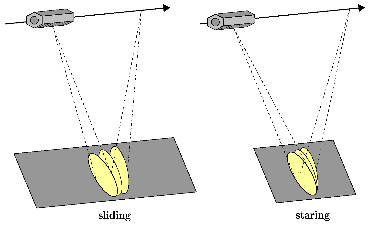
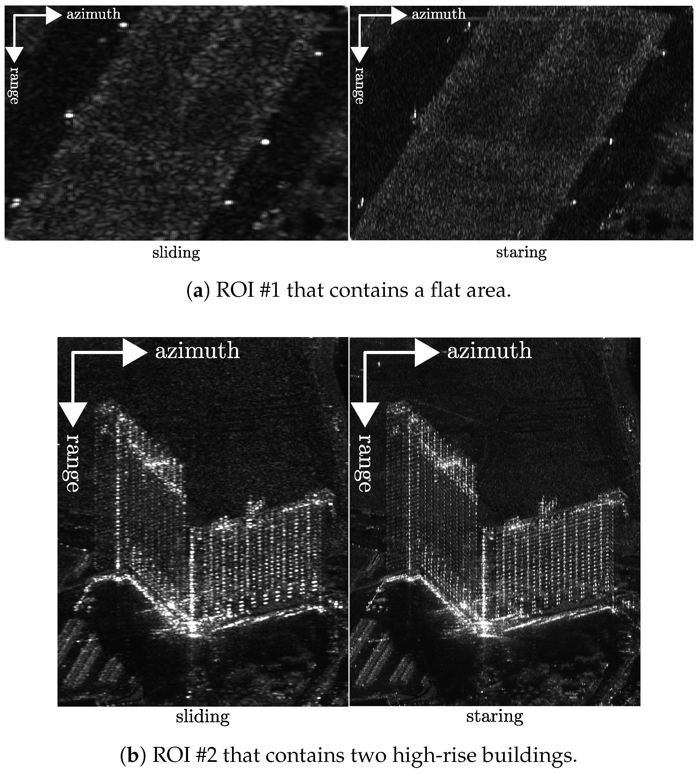
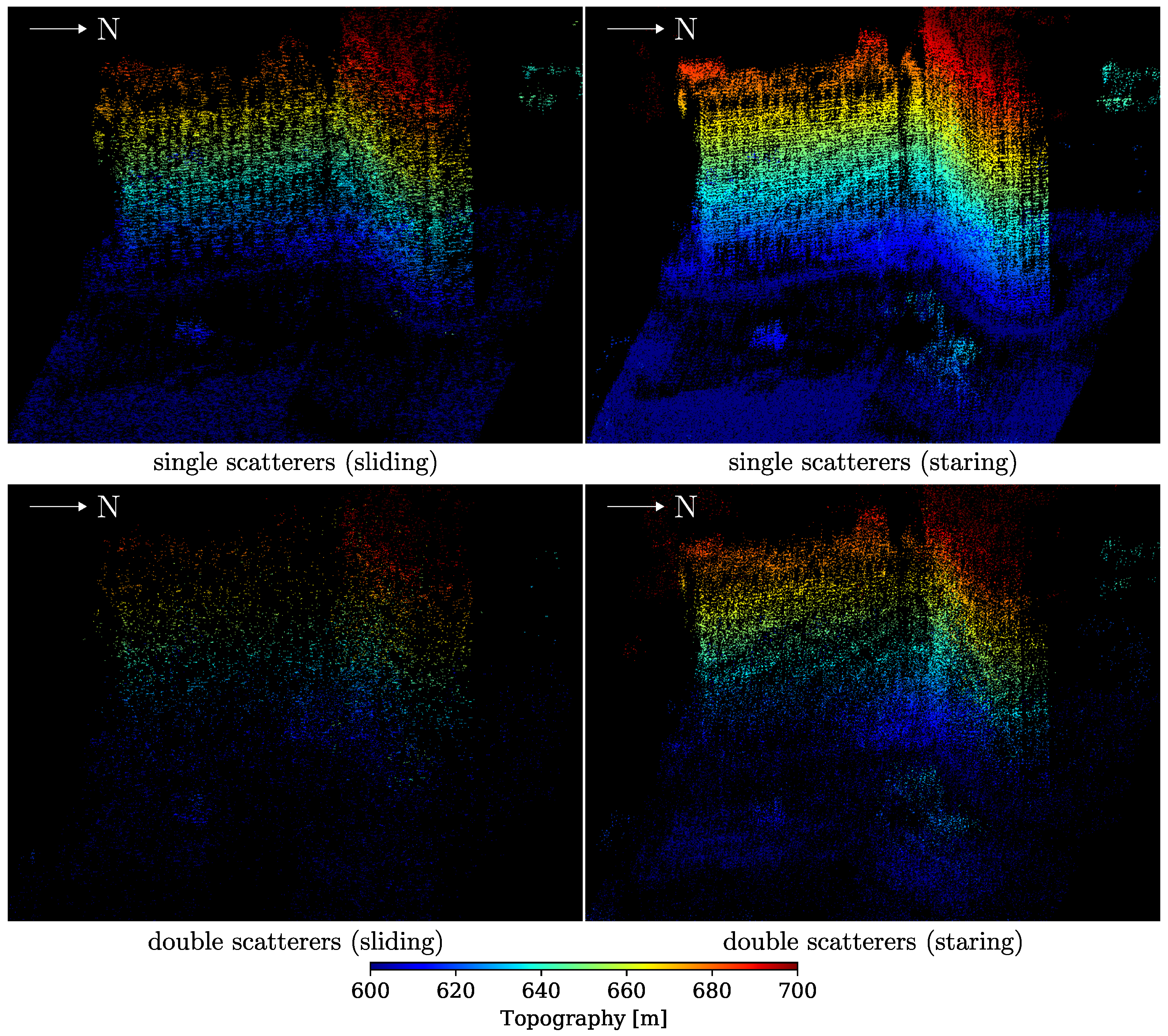
2.3.3. Staring Spotlight TomoSAR
2.3.4. Point Cloud Fusion
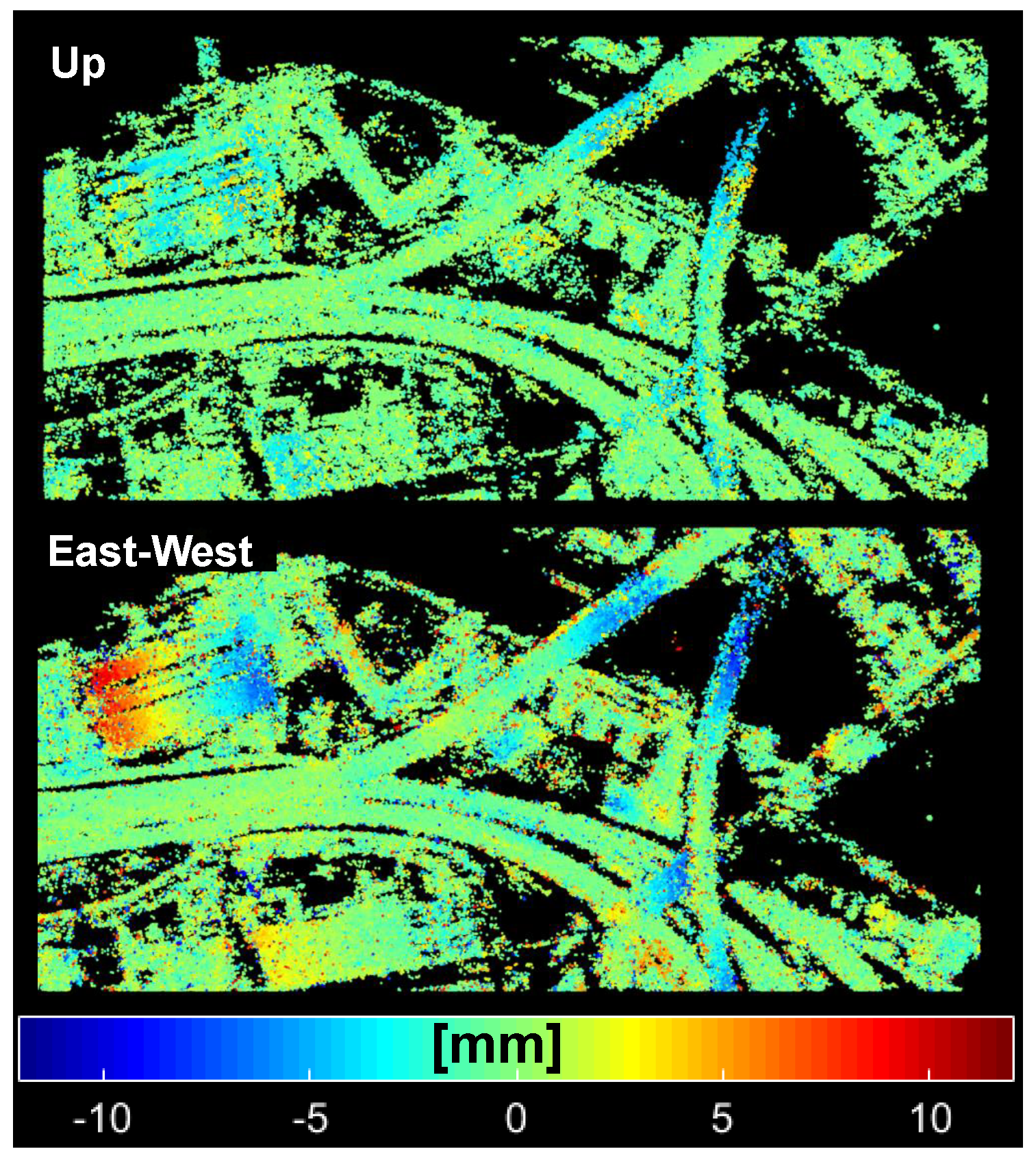
2.3.5. 3D Motion Decomposition
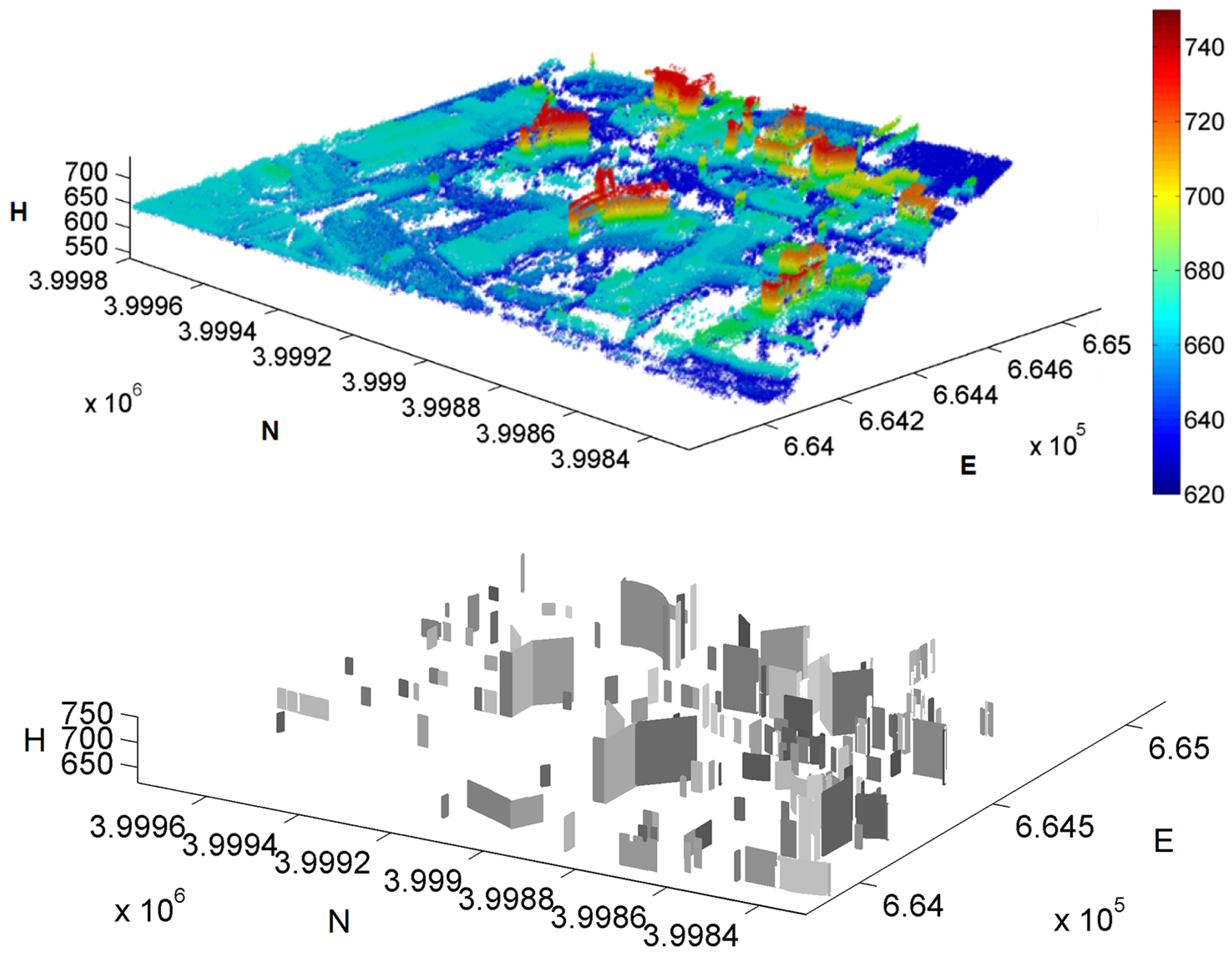
2.3.6. Object Reconstruction
2.4. Object-Based InSAR Algorithms
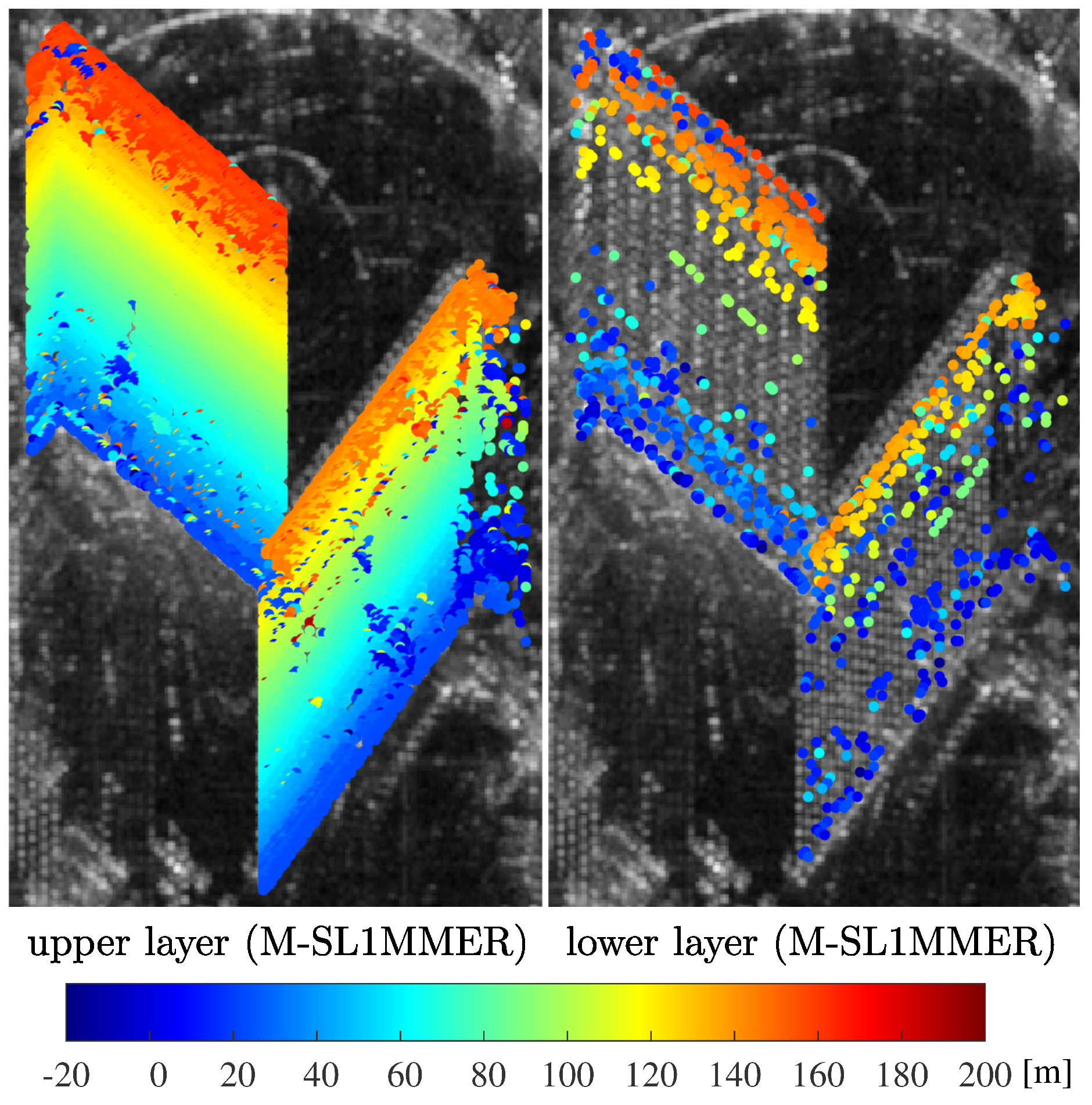
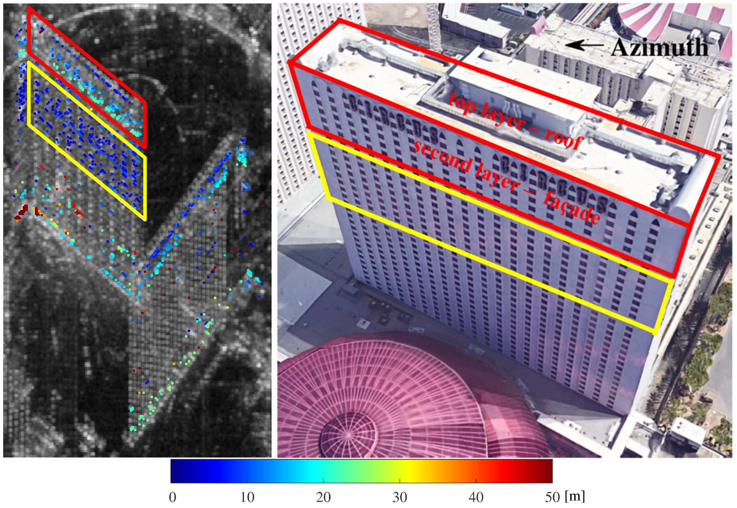
2.4.1. M-SL1MMER
2.4.2. RoMIO
3. Advances in Robust Estimation
3.1. Overview of Advances
- covariance matrix estimation for DS, due to the existence of non-Gaussian and nonstationary samples
- phase history parameters estimation for both DS and PS, due to observations with large unmodeled phase
3.2. Robust Covariance Matrix Estimation
- the selected samples are non-Gaussian (possibly heavily tailed distribution)
- the expected interferometric phase of the samples is nonstationary, e.g., very strong underlying topographic phase
3.2.1. Non-Gaussian Samples
3.2.2. Non-Gaussian Samples with Nonstationary Interferometric Phase
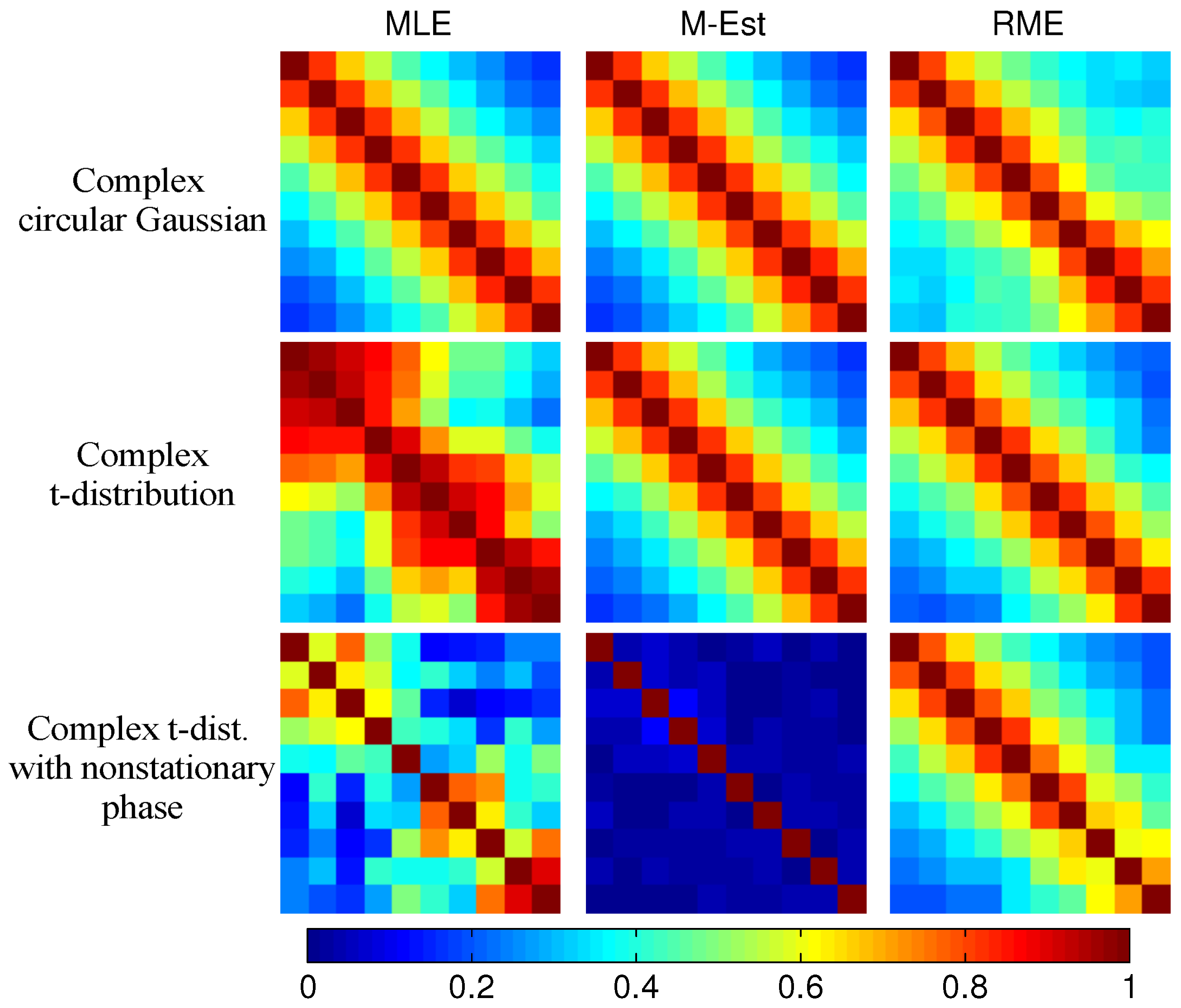
3.2.3. Comparison
3.3. Robust Phase History Parameters Retrieval
3.3.1. Robust PS Estimator
3.3.2. Robust DS Estimator
4. Advances in Absolute Positioning
4.1. Overview of Advances
4.2. Geodetic InSAR
4.2.1. SAR GCP Generation
- Step 1
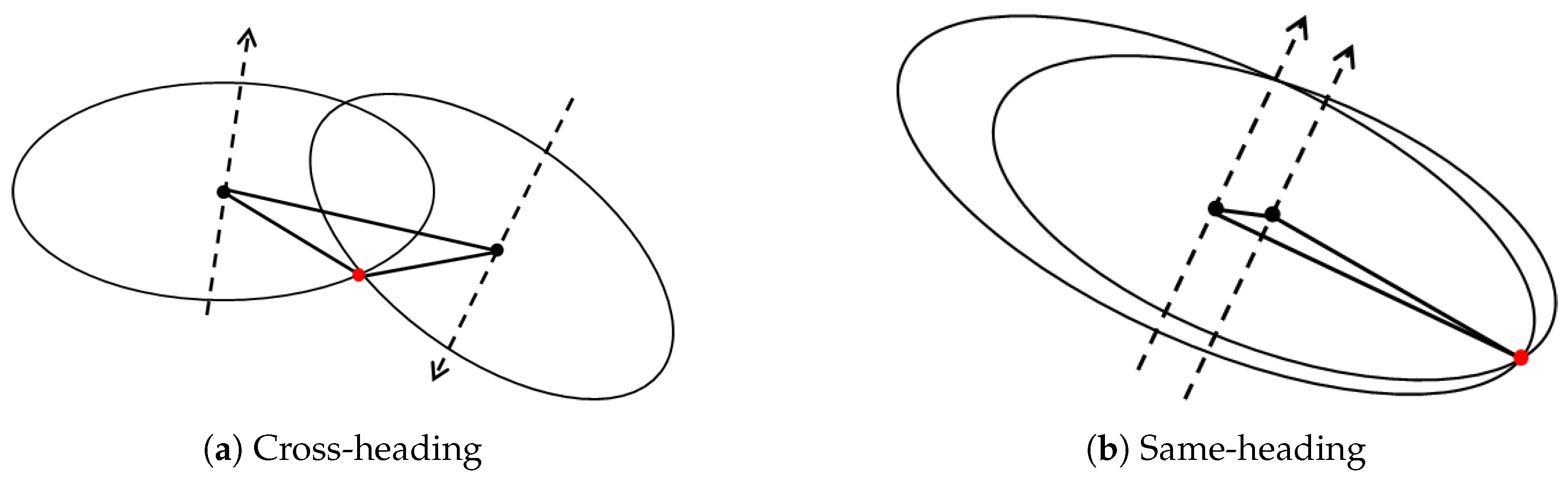
- Detection and matching of identical PS from SAR images acquired from different orbits. In the reference geodetic SAR tomography technique this task was performed manually [6]. At the current state of the framework, the identification of common PS can be carried out using the PSI multi-track fusion algorithm [39] for same-heading tracks and utilizing high resolution optical data [106] or external geospatial road network data [109] for cross-heading tracks. A combination of all the mentioned methods for automatic detection of large number of GCPs was used in [89].
- Step 2
- Step 3
- Step 4
- Correction of PS timings in the stack of images using imaging geodesy.
- Step 5
- Absolute 3D positioning of each PS by the stereo SAR method [82]. The posterior quality measures of the observations and the estimates are also reported in this step.
4.2.2. Absolute Localization of InSAR Point Clouds
4.2.3. Applications
5. Conclusions and Outlook
- Big data management technologies: So far, besides big missions, such as global TanDEM-X DEM generation, scientists are dealing with SAR data in the order of up to terabytes. However, this is about to change. Already today, petabytes of Sentinel-1 data are openly accessible to the public. Yet, only very limited groups are capable of national-scale InSAR data processing, to say nothing about global. To be prepared for the future, novel big geo-data management technologies are of high relevance.
- Fast and accurate parameter inversion algorithms: The development of inversion algorithms should keep up with the pace of data growth. For example, as a pre-study of Tandem-L, sequential interferometric phase estimators are proposed instead of full covariance matrix inversion to tackle the challenge of big InSAR data [72]. Fast solvers are demanded for many advanced parameter inversion models that often involve non-convex, nonlinear, and complex-valued optimization problem, such as CS-based tomographic inversion, or low rank complex tensor decomposition. Besides aforementioned model-based inversion methods, recently, data-driven machine learning/deep learning methods have boosted the baseline performances in many remote sensing problems [113], mostly in classification and detection tasks, yet its potential in InSAR processing or more generally in geoparamater estimation is not yet exploited at all. This deserves more attention of the community.
- Complicated motion: Up to now, only limited motion models, such as linear, seasonal or a combination of several basic models, are considered for deformation estimations of InSAR. There are also studies using model order selection to detect different types of motion either being embedded in the estimation [114] or considered as a post-processing [115]. However, the actual motion can be far more complex than any model can describe. The weekly repeat cycle and long-term monitoring capability of future sensors will enable retrieving much more complex motion models, and even allow performing classification of different types of motions and detecting anomalies. This calls for more sophisticated algorithms.
- Data assimilation: At present, the interferometric stack is usually a static cube of interferograms. As Sentinel-1 provides global coverage every six days, new stacking and multi-pass InSAR concepts should be able to include new images without excessive computational burden. This requires development of the data assimilation strategy, as well as novel inversion algorithms that only require the new measurements and the previous estimates for updating the parameters of interest.
- Multi-sensor data fusion: In the Copernicus era, it is standard that more than one data source, such as SAR and optical, is available at any test site. Intelligent use of the complementary peculiarities of the ever-increasing number of diverse remote sensing sensors and other geo-data sources has become the natural choice for many applications [116]. Some preliminary work in the community demonstrated that introducing the geometric prior or semantic prior to InSAR or TomoSAR reconstruction could significantly reduced the number of required SAR data while retaining the estimation accuracy [28,63]. This is definitely a promising future direction.
Author Contributions
Funding
Acknowledgments
Conflicts of Interest
Abbreviations
| ADI | Amplitude dispersion index |
| CCG | Complex circular Gaussian |
| CS | Compressive sensing |
| DEM | Digital elevation model |
| DS | Distributed scatterer |
| D-TomoSAR | Differential TomoSAR |
| ECMWF | European Center for Medium-Range Weather Forecasts |
| GCP | Ground control point |
| HRWS | High resolution wide swath |
| ICP | Iterative closest point |
| IERS | International Earth Rotation and Reference Systems Service |
| InSAR | SAR interferometry |
| LOS | Line of sight |
| MAP | Maximum a posteriori |
| MLE | Maximum likelihood estimator |
| M-SL1MMER | Multiple-snapshot SL1MMER |
| OSM | OpenStreetMap |
| Probability density function | |
| PSI | Persistent scatter interferometry |
| PS | Point/Persistent Scatterer |
| RIO | Robust InSAR optimization |
| RME | Rank M-estimator |
| ROI | Region of interest |
| ROMIO | Robust multi-pass InSAR via object-based low rank decomposition |
| SAR | Synthetic aperture radar |
| SCR | Signal-to-clutter ratio |
| SL1MMER | Scale-down by L1 norm minimization, model selection, and estimation reconstruction |
| SNR | Signal-to-noise ratio |
| TEC | Total electron content |
| TomoSAR | SAR tomography |
| VHR | Very high resolution |
References
- Hackel, S.; Montenbruck, O.; Steigenberger, P.; Balss, U.; Gisinger, C.; Eineder, M. Model improvements and validation of TerraSAR-X precise orbit determination. J. Geodesy 2017, 91, 547–562. [Google Scholar] [CrossRef]
- Hackel, S.; Gisinger, C.; Balss, U.; Wermuth, M.; Montenbruck, O. Long-Term Validation of TerraSAR-X Orbit Solutions with Laser and Radar Measurements. Remote Sens. 2018, 10, 762. [Google Scholar] [CrossRef]
- Zhu, X.X. Very High Resolution Tomographic SAR Inversion for Urban Infrastructure Monitoring—A Sparse and Nonlinear Tour. Ph.D. Thesis, Technische Universität München, München, Germany, 2011. [Google Scholar]
- Ferretti, A.; Fumagalli, A.; Novali, F.; Prati, C.; Rocca, F.; Rucci, A. A New Algorithm for Processing Interferometric Data-Stacks: SqueeSAR. IEEE Trans. Geosci. Remote Sens. 2011, 49, 3460–3470. [Google Scholar] [CrossRef]
- Wang, Y.; Zhu, X.X. Robust Estimators for Multipass SAR Interferometry. IEEE Trans. Geosci. Remote Sens. 2016, 54, 968–980. [Google Scholar] [CrossRef]
- Zhu, X.X.; Montazeri, S.; Gisinger, C.; Hanssen, R.F.; Bamler, R. Geodetic SAR Tomography. IEEE Trans. Geosci. Remote Sens. 2016, 54, 18–35. [Google Scholar] [CrossRef]
- Eineder, M.; Minet, C.; Steigenberger, P.; Cong, X.Y.; Fritz, T. Imaging Geodesy—Toward Centimeter-Level Ranging Accuracy with TerraSAR-X. IEEE Trans. Geosci. Remote Sens. 2011, 49, 661–671. [Google Scholar] [CrossRef]
- Zhu, X.X.; Bamler, R. Superresolving SAR Tomography for Multidimensional Imaging of Urban Areas: Compressive sensing-based TomoSAR inversion. IEEE Signal Process. Mag. 2014, 31, 51–58. [Google Scholar] [CrossRef]
- Bamler, R.; Hartl, P. Synthetic aperture radar interferometry. Inverse Probl. 1998, 14, R1. [Google Scholar] [CrossRef]
- Reigber, A.; Moreira, A. First demonstration of airborne SAR tomography using multibaseline L-band data. IEEE Trans. Geosci. Remote Sens. 2000, 38, 2142–2152. [Google Scholar] [CrossRef]
- Lombardini, F.; Montanari, M.; Gini, F. Reflectivity estimation for multibaseline interferometric radar imaging of layover extended sources. IEEE Trans. Signal Process. 2003, 51, 1508–1519. [Google Scholar] [CrossRef]
- Fornaro, G.; Serafino, F.; Soldovieri, F. Three-dimensional focusing with multipass SAR data. IEEE Trans. Geosci. Remote Sens. 2003, 41, 507–517. [Google Scholar] [CrossRef]
- Zhu, X. Spectral Estimation for Synthetic Aperture Radar Tomography. Master’s Thesis, Lehrstuhl für Methodik der Fernerkundung, TU München, Munich, Germany, 2008. [Google Scholar]
- Fornaro, G.; Reale, D.; Serafino, F. Four-dimensional SAR imaging for height estimation and monitoring of single and double scatterers. IEEE Trans. Geosci. Remote Sens. 2009, 47, 224–237. [Google Scholar] [CrossRef]
- Zhu, X.X.; Bamler, R. Very high resolution spaceborne SAR tomography in urban environment. IEEE Trans. Geosci. Remote Sens. 2010, 48, 4296–4308. [Google Scholar] [CrossRef] [Green Version]
- Zhu, X.X.; Bamler, R. Let’s do the time warp: Multicomponent nonlinear motion estimation in differential SAR tomography. IEEE Geosci. Remote Sens. Lett. 2011, 8, 735–739. [Google Scholar] [CrossRef] [Green Version]
- Crosetto, M.; Monserrat, O.; Cuevas-González, M.; Devanthéry, N.; Crippa, B. Persistent Scatterer Interferometry: A review. ISPRS J. Photogramm. Remote Sens. 2016, 115, 78–89. [Google Scholar] [CrossRef]
- Ferretti, A.; Prati, C.; Rocca, F. Permanent scatterers in SAR interferometry. IEEE Trans. Geosci. Remote Sens. 2001, 39, 8–20. [Google Scholar] [CrossRef] [Green Version]
- Adam, N.; Kampes, B.M.; Eineder, M. The development of a scientific persistent scatterer system: Modifications for mixed ERS/ENVISAT time series. In Proceedings of the Envisat and ERS Symposium, Salzburg, Austria, 6–10 September 2004; pp. 1–9. [Google Scholar]
- Kampes, B.M. Radar Interferometry: Persistent Scatterer Technique; Remote Sensing and Digital Image Processing; Springer: Dordrecht, The Netherlands, 2006. [Google Scholar]
- Van Leijen, F. Persistent Scatterer Interferometry Based on Geodetic Estimation Theory. Ph.D. Thesis, Delft University of Technology, Delft, The Netherlands, 2014. [Google Scholar]
- Wang, Y.; Zhu, X.X.; Bamler, R. An Efficient Tomographic Inversion Approach for Urban Mapping Using Meter Resolution SAR Image Stacks. IEEE Geosci. Remote Sens. Lett. 2014, 11, 1250–1254. [Google Scholar] [CrossRef] [Green Version]
- Rodriguez Gonzalez, F.; Bhutani, A.; Adam, N. L1 network inversion for robust outlier rejection in persistent Scatterer Interferometry. In Proceedings of the 2011 IEEE International Geoscience and Remote Sensing Symposium, Vancouver, BC, Canada, 24–29 July 2011; pp. 75–78. [Google Scholar] [CrossRef]
- Adam, N.; Gonzalez, F.R.; Parizzi, A.; Brcic, R. Wide area Persistent Scatterer Interferometry: Current developments, algorithms and examples. In Proceedings of the 2013 IEEE International Geoscience and Remote Sensing Symposium, Melbourne, VIC, Australia, 21–26 July 2013; pp. 1857–1860. [Google Scholar] [CrossRef]
- Rodriguez Gonzalez, F.; Adam, N.; Parizzi, A.; Brcic, R. The Integrated Wide Area Processor (IWAP): A Processor For Wide Area Persistent Scatterer Interferometry. In Proceedings of the ESA Living Planet Symposium 2013, Edinburgh, UK, 9–13 September 2013; pp. 1–4. [Google Scholar]
- Zhu, X.; Bamler, R. Very high Resolution SAR tomography via Compressive Sensing. In Proceedings of the Fringe 2009 Workshop, Frascati, Italy, 30 November–4 December 2009; pp. 1–7. [Google Scholar]
- Zhu, X.; Bamler, R. Tomographic SAR Inversion by L1-Norm Regularization—The Compressive Sensing Approach. IEEE Trans. Geosci. Remote Sens. 2010, 48, 3839–3846. [Google Scholar] [CrossRef]
- Zhu, X.X.; Ge, N.; Shahzad, M. Joint sparsity in SAR tomography for urban mapping. IEEE J. Sel. Top. Signal Process. 2015, 9, 1498–1509. [Google Scholar] [CrossRef]
- Pauciullo, A.; Reale, D.; De Maio, A.; Fornaro, G. Detection of Double Scatterers in SAR Tomography. IEEE Trans. Geosci. Remote Sens. 2012, 50, 3567–3586. [Google Scholar] [CrossRef]
- Zhu, X.X.; Bamler, R. Demonstration of Super-Resolution for Tomographic SAR Imaging in Urban Environment. IEEE Trans. Geosci. Remote Sens. 2012, 50, 3150–3157. [Google Scholar] [CrossRef] [Green Version]
- Zhu, X.; Bamler, R. Super-Resolution Power and Robustness of Compressive Sensing for Spectral Estimation With Application to Spaceborne Tomographic SAR. IEEE Trans. Geosci. Remote Sens. 2012, 50, 247–258. [Google Scholar] [CrossRef]
- Budillon, A.; Johnsy, A.C.; Schirinzi, G. A Fast Support Detector for Superresolution Localization of Multiple Scatterers in SAR Tomography. IEEE J. Sel. Top. Appl. Earth Obs. Remote Sens. 2017, 10, 1–12. [Google Scholar] [CrossRef]
- Ma, P.; Lin, H. Robust Detection of Single and Double Persistent Scatterers in Urban Built Environments. IEEE Trans. Geosci. Remote Sens. 2016, 54, 2124–2139. [Google Scholar] [CrossRef]
- Siddique, M.A.; Wegmüller, U.; Hajnsek, I.; Frey, O. Single-Look SAR Tomography as an Add-On to PSI for Improved Deformation Analysis in Urban Areas. IEEE Trans. Geosci. Remote Sens. 2016, 54, 6119–6137. [Google Scholar] [CrossRef]
- Shi, Y.; Zhu, X.X.; Yin, W.; Bamler, R. A fast and accurate basis pursuit denoising algorithm with application to super-resolving tomographic SAR. IEEE Trans. Geosci. Remote Sens. 2018, in press. [Google Scholar] [CrossRef]
- Gernhardt, S.; Bamler, R. Deformation monitoring of single buildings using meter-resolution SAR data in PSI. ISPRS J. Photogramm. Remote Sens. 2012, 73, 68–79. [Google Scholar] [CrossRef]
- Gernhardt, S.; Adam, N.; Hinz, S.; Bamler, R. Appearance of Persistent Scatterers for Different TerraSAR-X Acquisition Modes. In Proceedings of the ISPRS Workshop, Hannover, Germany, 2–5 June 2009; Volume XXXVIII-1-4-7/W5, pp. 1–5. [Google Scholar]
- Gernhardt, S.; Adam, N.; Eineder, M.; Bamler, R. Potential of very high resolution SAR for persistent scatterer interferometry in urban areas. Ann. GIS 2010, 16, 103–111. [Google Scholar] [CrossRef]
- Gernhardt, S.; Cong, X.Y.; Eineder, M.; Hinz, S.; Bamler, R. Geometrical Fusion of Multitrack PS Point Clouds. IEEE Geosci. Remote Sens. Lett. 2012, 9, 38–42. [Google Scholar] [CrossRef]
- Gernhardt, S. High Precision 3D Localization and Motion Analysis of Persistent Scatterers using Meter- Resolution Radar Satellite Data. Ph.D. Thesis, Technische Universität München, München, Germany, 2012. [Google Scholar]
- Kalia, A.C. Value-added Products in the Framework of the German Ground Motion Service. In Proceedings of the FRINGE 2017: 10th International Workshop on Advances in the Science and Applications of SAR Interferometry and Sentinel-1 InSAR, Helsinki, Finland, 5–9 June 2017. [Google Scholar]
- Zhu, X.X.; Wang, Y.; Gernhardt, S.; Bamler, R. Tomo-GENESIS: DLR’s tomographic SAR processing system. In Proceedings of the Joint Urban Remote Sensing (JURSE), Sao Paulo, Brazil, 2013; pp. 159–162. [Google Scholar] [CrossRef]
- Wang, Y.; Zhu, X.X. Automatic Feature-Based Geometric Fusion of Multiview TomoSAR Point Clouds in Urban Area. IEEE J. Sel. Top. Appl. Earth Obs. Remote Sens. 2015, 8, 953–965. [Google Scholar] [CrossRef]
- Zhu, X.X.; Shahzad, M. Facade Reconstruction Using Multiview Spaceborne TomoSAR Point Clouds. IEEE Trans. Geosci. Remote Sens. 2014, 52, 3541–3552. [Google Scholar] [CrossRef] [Green Version]
- Shahzad, M.; Zhu, X. Robust Reconstruction of Building Facades for Large Areas Using Spaceborne TomoSAR Point Clouds. IEEE Trans. Geosci. Remote Sens. 2015, 53, 752–769. [Google Scholar] [CrossRef] [Green Version]
- Shahzad, M.; Zhu, X.X. Automatic Detection and Reconstruction of 2-D/3-D Building Shapes from Spaceborne TomoSAR Point Clouds. IEEE Trans. Geosci. Remote Sens. 2016, 54, 1292–1310. [Google Scholar] [CrossRef]
- Wang, Y.; Zhu, X.X.; Bamler, R.; Gernhardt, S. Towards TerraSAR-X Street View: Creating City Point Cloud from Multi-Aspect Data Stacks. In Proceedings of the 2013 Joint Urban Remote Sensing Event (JURSE), Sao Paulo, Brazil, 21–23 April 2013; pp. 198–201. [Google Scholar] [CrossRef]
- Ge, N.; Rodriguez Gonzalez, F.; Wang, Y.; Zhu, X.X. Spaceborne Staring Spotlight SAR Tomography—A First Demonstration with TerraSAR-X. IEEE J. Sel. Top. Appl. Earth Obs. Remote Sens. 2018, in press. [Google Scholar]
- Eineder, M.; Adam, N.; Bamler, R.; Yague-Martinez, N.; Breit, H. Spaceborne spotlight SAR interferometry with TerraSAR-X. IEEE Trans. Geosci. Remote Sens. 2009, 47, 1524–1535. [Google Scholar] [CrossRef]
- Breit, H.; Fritz, T.; Balss, U.; Lachaise, M.; Niedermeier, A.; Vonavka, M. TerraSAR-X SAR processing and products. IEEE Trans. Geosci. Remote Sens. 2010, 48, 727–740. [Google Scholar] [CrossRef]
- Duque, S.; Breit, H.; Balss, U.; Parizzi, A. Absolute Height Estimation Using a Single TerraSAR-X Staring Spotlight Acquisition. IEEE Geosci. Remote Sens. Lett. 2015, 12, 1735–1739. [Google Scholar] [CrossRef]
- Bamler, R.; Eineder, M.; Adam, N.; Zhu, X.; Gernhardt, S. Interferometric Potential of High Resolution Spaceborne SAR. Photogramm. Fernerkund. Geoinf. 2009, 2009, 407–419. [Google Scholar] [CrossRef]
- Zhu, X.; Montazeri, S.; Gisinger, C.; Hanssen, R.; Bamler, R. Geodetic TomoSAR—Fusion of SAR Imaging Geodesy and TomoSAR for 3D Absolute Scatterer Positioning. In Proceedings of the 2014 IEEE International Geoscience and Remote Sensing Symposium (IGARSS), Quebec City, QC, Canada, 13–18 July 2014. [Google Scholar]
- Montazeri, S.; Zhu, X.X.; Eineder, M.; Bamler, R. Three-Dimensional Deformation Monitoring of Urban Infrastructure by Tomographic SAR Using Multitrack TerraSAR-X Data Stacks. IEEE Trans. Geosci. Remote Sens. 2016, 54, 6868–6878. [Google Scholar] [CrossRef]
- Montazeri, S. The Fusion of SAR Tomography and Stereo-SAR for 3D Absolute Scatterer Positioning. Master’s Thesis, Delft University of Technology, Delft, The Netherlands, 2014. [Google Scholar]
- Sun, Y.; Shahzad, M.; Zhu, X. First Prismatic Building Model Reconstruction from TomoSAR Point Clouds. ISPRS Int. Arch. Photogramm. Remote Sens. Spat. Inf. Sci. 2016, XLI-B3, 381–386. [Google Scholar] [CrossRef]
- Parizzi, A.; Brcic, R. Adaptive InSAR Stack Multilooking Exploiting Amplitude Statistics: A Comparison Between Different Techniques and Practical Results. IEEE Geosci. Remote Sens. Lett. 2011, 8, 441–445. [Google Scholar] [CrossRef]
- Wang, Y.; Zhu, X.; Bamler, R. Retrieval of Phase History Parameters from Distributed Scatterers in Urban Areas Using Very High Resolution SAR Data. ISPRS J. Photogramm. Remote Sens. 2012, 73, 89–99. [Google Scholar] [CrossRef]
- Deledalle, C.A.; Denis, L.; Tupin, F. NL-InSar: Nonlocal interferogram estimation. IEEE Trans. Geosci. Remote Sens. 2011, 49, 1441–1452. [Google Scholar] [CrossRef]
- Zhu, X.X.; Bamler, R.; Lachaise, M.; Adam, F.; Shi, Y.; Eineder, M. Improving TanDEM-X DEMs by Non-local InSAR Filtering. In Proceedings of the 10th European Conference on Synthetic Aperture Radar, Berlin, Germany, 2–6 June 2014; pp. 1–4. [Google Scholar]
- Baier, G.; Rossi, C.; Lachaise, M.; Zhu, X.X.; Bamler, R. Nonlocal InSAR filtering for high resolution DEM generation from TanDEM-X interferograms. IEEE Trans. Geosci. Remote Sens. 2018, in press. [Google Scholar] [CrossRef]
- Kang, J.; Wang, Y.; Körner, M.; Zhu, X. Robust Object-based Multi-pass InSAR Deformation Reconstruction. IEEE Trans. Geosci. Remote Sens. 2017, 55, 4239–4251. [Google Scholar] [CrossRef]
- Kang, J.; Wang, Y.; Schmitt, M.; Zhu, X.X. Object-based Multipass InSAR via Robust Low Rank Tensor Decomposition. IEEE Trans. Geosci. Remote Sens. 2018, 56, 3062–3077. [Google Scholar] [CrossRef]
- Aguilera, E.; Nannini, M.; Reigber, A. Multisignal compressed sensing for polarimetric SAR tomography. IEEE Geosci. Remote Sens. Lett. 2012, 9, 871–875. [Google Scholar] [CrossRef]
- Schmitt, M.; Stilla, U. Compressive sensing based layover separation in airborne single-pass multi-baseline InSAR data. IEEE Geosci. Remote Sens. Lett. 2013, 10, 313–317. [Google Scholar] [CrossRef]
- Fornaro, G.; Verde, S.; Reale, D.; Pauciullo, A. CAESAR: An approach based on covariance matrix decomposition to improve multibaseline–multitemporal interferometric SAR processing. IEEE Trans. Geosci. Remote Sens. 2015, 53, 2050–2065. [Google Scholar] [CrossRef]
- OpenStreetMap Contributors. Planet Dump. 2017. Available online: https://www.openstreetmap.org (accessed on 16 April 2018).
- Schmitt, M.; Schonberger, J.L.; Stilla, U. Adaptive Covariance Matrix Estimation for Multi-Baseline InSAR Data Stacks. IEEE Trans. Geosci. Remote Sens. 2014, 52, 1–11. [Google Scholar] [CrossRef]
- Samiei-Esfahany, S.; Martins, J.E.; van Leijen, F.; Hanssen, R.F. Phase Estimation for Distributed Scatterers in InSAR Stacks Using Integer Least Squares Estimation. IEEE Trans. Geosci. Remote Sens. 2016, 54, 5671–5687. [Google Scholar] [CrossRef]
- Cao, N.; Lee, H.; Jung, H.C. A Phase-Decomposition-Based PSInSAR Processing Method. IEEE Trans. Geosci. Remote Sens. 2016, 54, 1074–1090. [Google Scholar] [CrossRef]
- Even, M. A Study on Spatio-Temporal Filtering in the Spirit of SqueeSAR. In Proceedings of the 11th European Conference on Synthetic Aperture Radar (EUSAR), Hamburg, Germany, 6–9 June 2016; pp. 462–465. [Google Scholar]
- Ansari, H.; De Zan, F.; Bamler, R. Sequential Estimator: Toward Efficient InSAR Time Series Analysis. IEEE Trans. Geosci. Remote Sens. 2017, 55, 5637–5652. [Google Scholar] [CrossRef]
- Verde, S.; Reale, D.; Pauciullo, A.; Fornaro, G. Improved Small Baseline processing by means of CAESAR eigen-interferograms decomposition. ISPRS J. Photogramm. Remote Sens. 2018, 139, 1–13. [Google Scholar] [CrossRef]
- Even, M.; Schulz, K. InSAR Deformation Analysis with Distributed Scatterers: A Review Complemented by New Advances. Remote Sens. 2018, 10, 744. [Google Scholar] [CrossRef]
- Ollila, E.; Koivunen, V. Influence functions for array covariance matrix estimators. In Proceedings of the 2003 IEEE Workshop on Statistical Signal Processing, St. Louis, MO, USA, 28 September–1 October 2003; pp. 462–465. [Google Scholar]
- Zoubir, A.M.; Koivunen, V.; Chakhchoukh, Y.; Muma, M. Robust Estimation in Signal Processing: A Tutorial-Style Treatment of Fundamental Concepts. IEEE Signal Process. Mag. 2012, 29, 61–80. [Google Scholar] [CrossRef]
- Visuri, S.; Koivunen, V.; Oja, H. Sign and rank covariance matrices. J. Stat. Plan. Inference 2000, 91, 557–575. [Google Scholar] [CrossRef] [Green Version]
- Croux, C.; Ollila, E.; Oja, H. Sign and rank covariance matrices: Statistical properties and application to principal components analysis. In Statistical Data Analysis Based on the L1-Norm and Related Methods; Springer: Basel, Switzerland, 2002; pp. 257–269. [Google Scholar]
- Rife, D.; Boorstyn, R.R. Single tone parameter estimation from discrete-time observations. IEEE Trans. Inf. Theory 1974, 20, 591–598. [Google Scholar] [CrossRef]
- De Zan, F. Optimizing SAR Interferometry for Decorrelating Scatterers. Ph.D. Thesis, Politecnico di Milano, Milan, Italy, 2008. [Google Scholar]
- Cong, X.Y.; Balss, U.; Eineder, M.; Fritz, T. Imaging Geodesy—Centimeter-Level Ranging Accuracy with TerraSAR-X: An Update. IEEE Geosci. Remote Sens. Lett. 2012, 9, 948–952. [Google Scholar] [CrossRef]
- Gisinger, C.; Balss, U.; Pail, R.; Zhu, X.X.; Montazeri, S.; Gernhardt, S.; Eineder, M. Precise Three-Dimensional Stereo Localization of Corner Reflectors and Persistent Scatterers with TerraSAR-X. IEEE Trans. Geosci. Remote Sens. 2015, 53, 1782–1802. [Google Scholar] [CrossRef]
- Yoon, Y.; Eineder, M.; Yague-Martinez, N.; Montenbruck, O. TerraSAR-X Precise Trajectory Estimation and Quality Assessment. IEEE Trans. Geosci. Remote Sens. 2009, 47, 1859–1868. [Google Scholar] [CrossRef]
- Breit, H.; Börner, E.; Mittermayer, J.; Holzner, J.; Eineder, M. The TerraSAR-X Multi-Mode SAR Processor—Algorithms and Design. In Proceedings of the 5th European Conference on Synthetic Aperture Radar, Ulm, Germany, 25–27 May 2004. [Google Scholar]
- Cumming, I.G.; Wong, F.H.C. Digital Processing of Synthetic Aperture Radar Data: Algorithms and Implementation; Artech House Remote Sensing Library: Boston, MA, USA, 2005. [Google Scholar]
- Balss, U.; Cong, X.Y.; Brcic, R.; Rexer, M.; Minet, C.; Breit, H.; Eineder, M.; Fritz, T. High precision measurement on the absolute localization accuracy of TerraSAR-X. In Proceedings of the 2012 IEEE International Geoscience and Remote Sensing Symposium (IGARSS), Munich, Germany, 22–27 July 2012; pp. 1625–1628. [Google Scholar] [CrossRef]
- Eineder, M.; Balss, U.; Suchandt, S.; Gisinger, C.; Cong, X.; Runge, H. A definition of next-generation SAR products for geodetic applications. In Proceedings of the 2015 IEEE International Geoscience and Remote Sensing Symposium (IGARSS), Milan, Italy, 26–31 July 2015; pp. 1638–1641. [Google Scholar] [CrossRef]
- Petit, G.; Luzum, B. IERS Conventions; IERS Technical Note No. 36; Verlag des Bundesamts für Kartographie und Geodäsie: Frankfurt am Main, Germany, 2010. [Google Scholar]
- Montazeri, S.; Gisinger, C.; Eineder, M.; Zhu, X.X. Automatic Detection and Positioning of Ground Control Points Using TerraSAR-X Multiaspect Acquisitions. IEEE Trans. Geosci. Remote Sens. 2018, 56, 2613–2632. [Google Scholar] [CrossRef]
- Schubert, A.; Jehle, M.; Small, D.; Meier, E. Influence of Atmospheric Path Delay on the Absolute Geolocation Accuracy of TerraSAR-X High-Resolution Products. IEEE Trans. Geosci. Remote Sens. 2010, 48, 751–758. [Google Scholar] [CrossRef] [Green Version]
- Gisinger, C. Atmospheric Corrections for TerraSAR-X Derived from GNSS Observations. Master’s Thesis, Technische Universität München, München, Germany, 2012. [Google Scholar]
- Balss, U.; Breit, H.; Fritz, T.; Steinbrecher, U.; Gisinger, C.; Eineder, M. Analysis of internal timings and clock rates of TerraSAR-X. In Proceedings of the 2014 IEEE International Geoscience and Remote Sensing Symposium (IGARSS), Quebec City, QC, Canada, 13–18 July 2014; pp. 2671–2674. [Google Scholar] [CrossRef]
- Schubert, A.; Jehle, M.; Small, D.; Meier, E. Mitigation of atmospheric perturbations and solid Earth movements in a TerraSAR-X time-series. J. Geodesy 2012, 86, 257–270. [Google Scholar] [CrossRef]
- Balss, U.; Gisinger, C.; Cong, X.; Eineder, M.; Fritz, T.; Breit, H.; Brcic, R. GNSS-Based Signal Path Delay and Geodynamic Corrections for Centimeter Level Pixel Localization with TerraSAR-X. In Proceedings of the 5th TerraSAR-X Science Team Meeting, Oberpfaffenhofen, Germany, 10–14 June 2013; pp. 1–4. [Google Scholar]
- Balss, U.; Gisinger, C.; Cong, X.Y.; Brcic, R.; Hackel, S.; Eineder, M. Precise measurements on the absolute localization accuracy of TerraSAR-X on the base of far-distributed test sites. In Proceedings of the EUSAR 2014: 10th European Conference on Synthetic Aperture Radar, Berlin, Germany, 2–4 June 2014. [Google Scholar]
- Eineder, M.; Balss, U.; Biarge, S.D. Water level measurement by controlled radar reflection and TerraSAR-X imaging geodesy. In Proceedings of the 2014 IEEE International Geoscience and Remote Sensing Symposium (IGARSS), Quebec City, QC, Canada, 13–18 July 2014; pp. 5141–5143. [Google Scholar] [CrossRef]
- Duque, S.; Balss, U.; Cong, X.Y.; Yague-Martinez, N.; Fritz, T. Absolute Ranging for Maritime Applications using TerraSAR-X and TanDEM-X Data. In Proceedings of the EUSAR 2014: 10th European Conference on Synthetic Aperture Radar, Berlin, Germany, 2–4 June 2014; pp. 1–4. [Google Scholar]
- Eineder, M.; Gisinger, C.; Balss, U.; Cong, X.Y.; Montazeri, S.; Hackel, S.; Rodriguez Gonzalez, F.; Runge, H. SAR Imaging Geodesy—Recent Results for TerraSAR-X and for Sentinel-1. In Proceedings of the FRINGE 2017: 10th International Workshop on Advances in the Science and Applications of SAR Interferometry and Sentinel-1 InSAR, Helsinki, Finland, 5–9 June 2017. [Google Scholar]
- Balss, U.; Gisinger, C.; Cong, X.; Eineder, M.; Brcic, R. Precise 2-D and 3-D Ground Target Localization with TerraSAR-X. ISPRS Int. Arch. Photogramm. Remote Sens. Spat. Inf. Sci. 2013, XL-1/W, 23–28. [Google Scholar] [CrossRef]
- Eldhuset, K.; Weydahl, D.J. Geolocation and Stereo Height Estimation Using TerraSAR-X Spotlight Image Data. IEEE Trans. Geosci. Remote Sens. 2011, 49, 3574–3581. [Google Scholar] [CrossRef]
- Raggam, H.; Perko, R.; Gutjahr, K.; Kiefl, N.; Koppe, W.; Hennig, S. Accuracy Assessment of 3D Point Retrieval from TerraSAR-X Data Sets. In Proceedings of the 8th European Conference on Synthetic Aperture Radar, Aachen, Germany, 7–10 June 2010; pp. 1–4. [Google Scholar]
- Koppe, W.; Wenzel, R.; Hennig, S.; Janoth, J.; Hummel, P.; Raggam, H. Quality assessment of TerraSAR-X derived ground control points. In Proceedings of the 2012 IEEE International Geoscience and Remote Sensing Symposium (IGARSS), Munich, Germany, 22–27 July 2012; pp. 3580–3583. [Google Scholar] [CrossRef]
- Gisinger, C.; Gernhardt, S.; Auer, S.; Balss, U.; Hackel, S.; Pail, R.; Eineder, M. Absolute 4-D positioning of persistent scatterers with TerraSAR-X by applying geodetic stereo SAR. In Proceedings of the 2015 IEEE International Geoscience and Remote Sensing Symposium (IGARSS), Milan, Italy, 26–31 July 2015; pp. 2991–2994. [Google Scholar] [CrossRef]
- Gisinger, C.; Montazeri, S.; Balss, U.; Cong, X.Y.; Hackel, S.; Zhu, X.X.; Pail, R.; Eineder, M. Applying geodetic SAR with TerraSAR-X and TanDEM-X. In Proceedings of the TerraSAR-X/TanDEM-X Science Team Meeting, Oberpfaffenhofen, Germany, 17–20 October 2016. [Google Scholar]
- Runge, H.; Balss, U.; Suchandt, S.; Klarner, R.; Cong, X. DriveMark – Generation of High Resolution Road Maps with Radar Satellites. In Proceedings of the 11th ITS European Congress, Glasgow, Scotland, 6–9 June 2016; pp. 1–6. [Google Scholar]
- Montazeri, S.; Zhu, X.X.; Balss, U.; Gisinger, C.; Wang, Y.; Eineder, M.; Bamler, R. SAR ground control point identification with the aid of high resolution optical data. In Proceedings of the 2016 IEEE International Geoscience and Remote Sensing Symposium (IGARSS), Beijing, China, 10–15 July 2016; pp. 3205–3208. [Google Scholar] [CrossRef]
- Balss, U.; Runge, H.; Suchandt, S.; Cong, X.Y. Automated extraction of 3-D Ground Control Points from SAR images—An upcoming novel data product. In Proceedings of the 2016 IEEE International Geoscience and Remote Sensing Symposium (IGARSS), Beijing, China, 10–15 July 2016; pp. 5023–5026. [Google Scholar] [CrossRef]
- Nitti, D.O.; Morea, A.; Nutricato, R.; Chiaradia, M.T.; La Mantia, C.; Agrimano, L.; Samarelli, S. Automatic GCP extraction with high resolution COSMO-SkyMed products. In Proceedings of the SPIE Remote Sensing 2016, Edinburgh, UK, 26–29 September 2016; Volume 10003. [Google Scholar] [CrossRef]
- Montazeri, S.; Gisinger, C.; Zhu, X.X.; Eineder, M.; Bamler, R. Automatic positioning of SAR ground control points from multi-aspect TerraSAR-X acquisitions. In Proceedings of the 2017 IEEE International Geoscience and Remote Sensing Symposium (IGARSS), Fort Worth, TX, USA, 23–28 July 2017; pp. 961–964. [Google Scholar] [CrossRef]
- Hubert, M.; Vandervieren, E. An adjusted boxplot for skewed distributions. Comput. Stat. Data Anal. 2008, 52, 5186–5201. [Google Scholar] [CrossRef]
- Montazeri, S.; Zhu, X.X.; Gisinger, C.; Rodriguez Gonzalez, F.; Eineder, M.; Bamler, R. Towards Absolute Positioning of InSAR Point Clouds. In Proceedings of the FRINGE 2017: 10th International Workshop on Advances in the Science and Applications of SAR Interferometry and Sentinel-1 InSAR, Helsinki, Finland, 5–9 June 2017. [Google Scholar]
- Wang, Y.; Zhu, X.X.; Zeisl, B.; Pollefeys, M. Fusing Meter-Resolution 4-D InSAR Point Clouds and Optical Images for Semantic Urban Infrastructure Monitoring. IEEE Trans. Geosci. Remote Sens. 2017, 55, 14–26. [Google Scholar] [CrossRef] [Green Version]
- Zhu, X.X.; Tuia, D.; Mou, L.; Xia, G.S.; Zhang, L.; Xu, F.; Fraundorfer, F. Deep Learning in Remote Sensing: A Comprehensive Review and List of Resources. IEEE Geosci. Remote Sens. Mag. 2017, 5, 8–36. [Google Scholar] [CrossRef] [Green Version]
- Ge, N.; Zhu, X. Bistatic-like Differential SAR Tomography—A Preliminary Framework for Tandem-L. IEEE Trans. Geosci. Remote Sens. 2018. submitted. [Google Scholar]
- Chang, L.; Hanssen, R.F. A Probabilistic Approach for InSAR Time-Series Postprocessing. IEEE Trans. Geosci. Remote Sens. 2016, 54, 421–430. [Google Scholar] [CrossRef]
- Schmitt, M.; Zhu, X.X. Data Fusion and Remote Sensing: An ever-growing relationship. IEEE Geosci. Remote Sens. Mag. 2016, 4, 6–23. [Google Scholar] [CrossRef]


| Density (thousand/km) | |
|---|---|
| PSI [38] | 40–100 |
| D-TomoSAR (non-superresolving) [15] | 150–250 |
| D-TomoSAR (SL1MMER) [48] | 500–1500 |
| Sliding | Staring | Ratio | |
|---|---|---|---|
| No. of single scatterers | |||
| No. of double scatterers | |||
| Total no. of scatterers | |||
| Single-to-double-scatterer ratio | |||
| Scatterer density (million/km) |
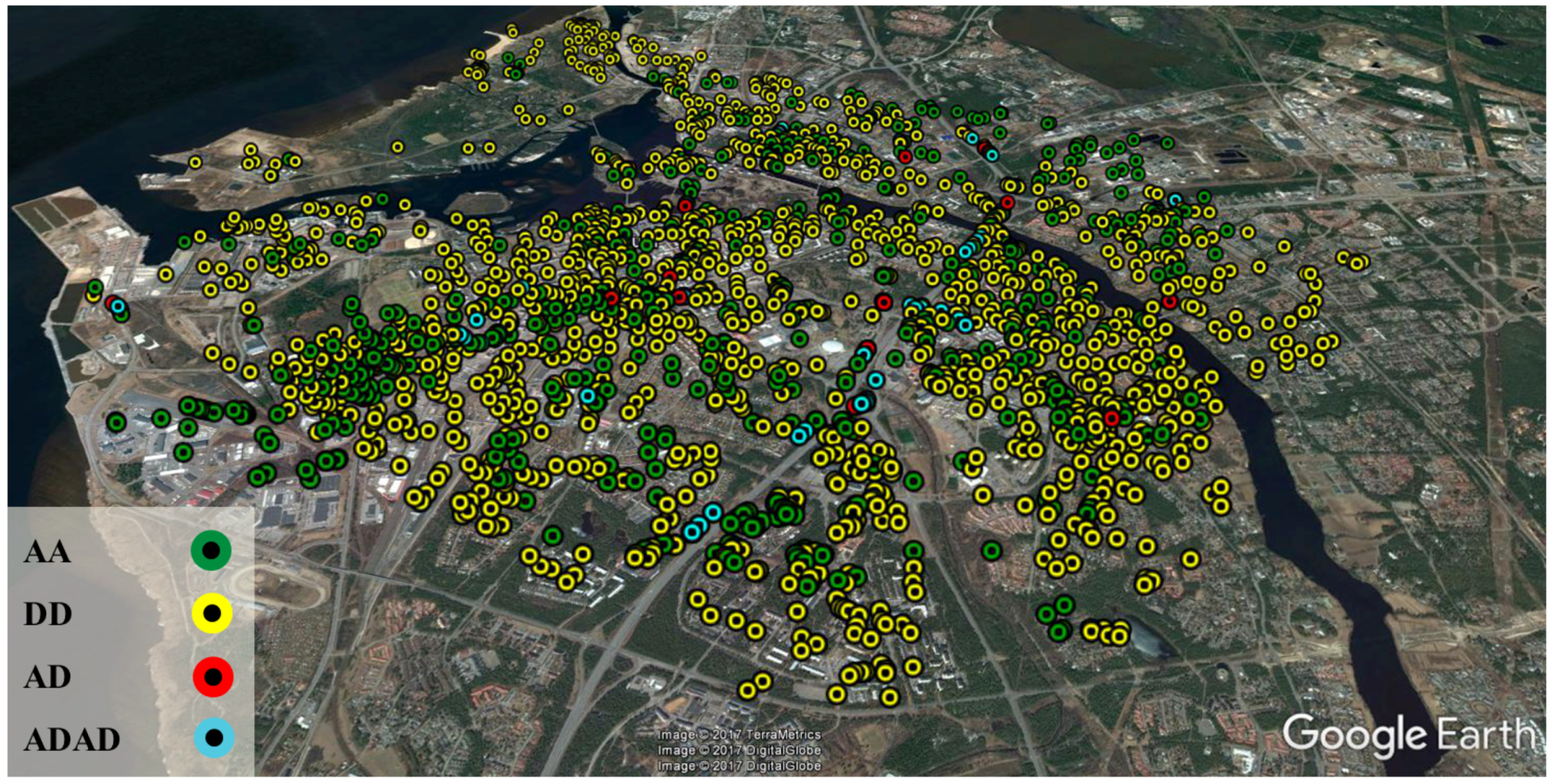
| Geometry | Number of Scatterers | ||||||
|---|---|---|---|---|---|---|---|
| AA | 565 | 17.73 | 5.04 | 15.87 | 11.98 | 2.63 | 11.09 |
| DD | 1417 | 15.08 | 3.80 | 16.71 | 10.38 | 2.10 | 11.30 |
| AD | 24 | 2.26 | 2.50 | 1.75 | 0.99 | 1.11 | 0.83 |
| ADAD | 43 | 1.17 | 1.40 | 1.12 | 0.42 | 0.55 | 0.37 |
© 2018 by the authors. Licensee MDPI, Basel, Switzerland. This article is an open access article distributed under the terms and conditions of the Creative Commons Attribution (CC BY) license (http://creativecommons.org/licenses/by/4.0/).
Share and Cite
Zhu, X.X.; Wang, Y.; Montazeri, S.; Ge, N. A Review of Ten-Year Advances of Multi-Baseline SAR Interferometry Using TerraSAR-X Data. Remote Sens. 2018, 10, 1374. https://doi.org/10.3390/rs10091374
Zhu XX, Wang Y, Montazeri S, Ge N. A Review of Ten-Year Advances of Multi-Baseline SAR Interferometry Using TerraSAR-X Data. Remote Sensing. 2018; 10(9):1374. https://doi.org/10.3390/rs10091374
Chicago/Turabian StyleZhu, Xiao Xiang, Yuanyuan Wang, Sina Montazeri, and Nan Ge. 2018. "A Review of Ten-Year Advances of Multi-Baseline SAR Interferometry Using TerraSAR-X Data" Remote Sensing 10, no. 9: 1374. https://doi.org/10.3390/rs10091374
APA StyleZhu, X. X., Wang, Y., Montazeri, S., & Ge, N. (2018). A Review of Ten-Year Advances of Multi-Baseline SAR Interferometry Using TerraSAR-X Data. Remote Sensing, 10(9), 1374. https://doi.org/10.3390/rs10091374