Article

Merging Unmanned Aerial Systems (UAS) Imagery and Echo Soundings with an Adaptive Sampling Technique for Bathymetric Surveys

by
Laura V. Alvarez
1,2,*,
Hernan A. Moreno
3,4,
Antonio R. Segales
1,5,
Tri G. Pham
4,
Elizabeth A. Pillar-Little
1,2 and
Phillip B. Chilson
1,2
1
Center for Autonomous Sensing and Sampling, University of Oklahoma, Norman, OK 73072, USA
2
School of Meteorology, University of Oklahoma, Norman, OK 73072, USA
3
Department of Geography and Environmental Sustainability, University of Oklahoma, Norman, OK 73019, USA
4
School of Civil Engineering and Environmental Science, University of Oklahoma, Norman, OK 73019, USA
5
School of Electrical and Computer Engineering, University of Oklahoma, Norman, OK 73019, USA
*
Author to whom correspondence should be addressed.
Remote Sens. 2018, 10(9), 1362; https://doi.org/10.3390/rs10091362
Submission received: 19 July 2018 / Revised: 15 August 2018 / Accepted: 21 August 2018 / Published: 28 August 2018
(This article belongs to the Special Issue Remote Sensing from Unmanned Aerial Vehicles (UAVs))

Abstract

:
Bathymetric surveying to gather information about depths and underwater terrain is increasingly important to the sciences of hydrology and geomorphology. Submerged terrain change detection, water level, and reservoir storage monitoring demand extensive bathymetric data. Despite often being scarce or unavailable, this information is fundamental to hydrodynamic modeling for imposing boundary conditions and building computational domains. In this manuscript, a novel, low-cost, rapid, and accurate method is developed to measure submerged topography, as an alternative to conventional approaches that require significant economic investments and human power. The method integrates two types of Unmanned Aerial Systems (UAS) sampling techniques. The first couples a small UAS (sUAS) to an echosounder attached to a miniaturized boat for surveying submerged topography in deeper water within the range of accuracy. The second uses Structure from Motion (SfM) photogrammetry to cover shallower water areas no detected by the echosounder where the bed is visible from the sUAS. The refraction of light passing through air–water interface is considered for improving the bathymetric results. A zonal adaptive sampling algorithm is developed and applied to the echosounder data to densify measurements where the standard deviation of clustered points is high. This method is tested at a small reservoir in the U.S. southern plains. Ground Control Points (GCPs) and checkpoints surveyed with a total station are used for properly georeferencing of the SfM photogrammetry and assessment of the UAS imagery accuracy. An independent validation procedure providing a number of skill and error metrics is conducted using ground-truth data collected with a leveling rod at co-located reservoir points. Assessment of the results shows a strong correlation between the echosounder, SfM measurements and the field observations. The final product is a hybrid bathymetric survey resulting from the merging of SfM photogrammetry and echosoundings within an adaptive sampling framework.

Graphical Abstract

1. Introduction

1.1. Introduction and Overview

For decades, topographic and bathymetric surveys have been widely used to study the evolution of landscapes and geomorphological processes. With the advent of new monitoring and modeling systems, interest in high-resolution topographic data has rapidly increased in a broad spectrum of sciences. In hydrologic and geomorphologic sciences, specific applications of high-resolution topographic data include but are not limited to the study of terrain change and detection of landslides [1,2,3,4,5], fluvial modeling [6,7], distributed hydrologic modeling [8,9,10,11], habitat assessment, and river restoration [12,13,14,15,16,17]. A broad range of techniques to measure bathymetry have evolved to meet measurement requirements, across different disciplines. Existing approaches range from traditional total stations and leveling equipment [4,18] to novel and developing techniques such as digital photogrammetry [19,20,21,22,23], terrestrial laser scanning, and aerial Light Detection And Ranging (LiDAR) [1,24,25,26,27,28]. Despite the range of available methods, the production of Digital Elevation Models (DEMs) demands significant investments of resources including expensive equipment, hardware, software, and manpower [29,30,31]. Remote sensing technology utilizing Unmanned Aircraft Systems (UAS) represents a cost-effective alternative to conventional methods that has been gaining adepts in the earth science community during the last decade [2,32,33,34,35,36,37].
Unmanned Aerial Vehicles (UAV), also known as aerial robots or drones, are aircrafts piloted by remote control rather than by a human pilot. When taken as a collective system of components (UAV, ground station, telemetry, etc.), the term UAS is used. Small unmanned aircraft systems (sUAS) are UAS that weigh less than 25 kg and have integrated autopilot technology that allows for semi- or fully-autonomous navigation, flight control, and image acquisition capabilities [38,39,40,41]. sUAS are currently used for the acquisition of photogrammetrically-derived DEMs [33,35,37,38,42,43,44,45]. Image acquisition with off-the-shelf cameras mounted in sUAS can be performed at a spatial resolution on the order of meters to centimeters [2,29,30,34,36,45]. The accuracy of DEMs based on aerial imagery is found to be comparable to aerial LiDAR data [29]. While high-resolution topographic surveying has traditionally been associated with high costs of data collection (e.g., traditional airbone LiDAR) [24,26,29,37], sUAS imagery provides a low-cost yet accurate alternative to DEM construction [35,36,43,46]. Recently, studies have been utilizing sUAS to collect terrain datasets examining topics such as landslides [2], Aeolian and glacial landforms [38,47], riparian forests [33] and fluvial geomorphology [30,48]. Nonetheless, few studies have applied sUAS imagery to quantify submerged topography in water bodies, such as rivers, swamps, marshes, lakes and reservoirs [29,37,49].
Submerged topography is essential to understanding the hydrologic and geomorphologic processes of lotic and lentic systems. In lentic systems, traditional techniques for examining bathymetry include cross-section surveys along river reaches [4,18]. Nevertheless, this conventional method is time-demanding, limited due to accessibility, and constrained to small to medium-size rivers. Indirect methods of estimating the bathymetry of water bodies have been expanding since the development and implementation of acoustic sensing technologies [17,50,51,52,53,54,55,56,57]. Acoustic instruments aim to replace conventional techniques to measure submerged topography and velocity profiles. Single-beam and multi-beam echosounders and Acoustic Doppler Current Profilers (ADCP) are currently utilized for acquiring point cloud bathymetry [54]. While acoustic sensing technologies have been applied to the detection of ocean and coastal bathymetric changes [17,25,51,57,58], the use of these technologies has been limited in fluvial geomorphology [50,54,55,56,59,60,61].

1.2. Conventional and Emerging Techniques for Bathymetric Surveying

1.2.1. Total-Station Surveying

Total station theodolite (TST) or total station surveys use electronic survey equipment in conjunction with a measuring tape, level, and rod to record the terrain by measuring distances, azimuth and elevation [62]. This technique is mainly applied in civil engineering, [63,64,65,66], and mining [67,68], although it has been widely applied in earth sciences with demonstrated high accuracy in rugged terrains [4,18,69]. The accuracy of TST surveys can reach a point spacing of +/− 0.05 m within an area of 0.075 to 0.275 m 2 [62]. Due to its accuracy, TST surveys are commonly used as ground control points (GCP) for remote sensing mapping [3,29,37]. However, producing a DEM using TST surveying requires significant monetary investment and human power. Additionally, this technique is limited to channel cross section surveys that lack the ability to measure 3D maps. This makes TST an insufficient method for providing large scale and continuous data to quantify the spatial and temporal variability of submerged topography.

1.2.2. Terrestrial and Aerial LiDAR

LiDAR uses differences in laser return times and wavelengths to make a 3D representation of terrain targets from a station or moving vehicle (terrestrial LiDAR) or attached to an aircraft (airborne LiDAR) [24]. Terrestrial LiDAR is very accurate and commonly used for high resolution topographic surveys of exposed terrain [35,70]. However, ground-based LiDAR systems are very expensive, require significant human power to operate and maintain, and provide limited spatial coverage [29,30,31].
The use of airborne LiDAR has rapidly grown over the last two decades, with numerous applications for examining hydrologic and geomorphologic processes such as the detection of landslides [40], estimation of vegetation cover [71,72,73], assessment of forest and canopy height [74,75,76,77,78,79], and urban scene classification [80,81,82]. The use of LiDAR in underwater mapping applications has been limited [24] mainly because the near-infrared energy utilized by LiDAR instruments is lost due to absorption at the water, making it ineffective at probing underwater elevations [37,47]. Emerging techniques employ a blue-green laser to determine the air–water interface in clear, shallow water [27,28,83,84,85]. This technology has been intensively developed since the mid-1990s, providing high-density, remote data, for bathymetry up to 10 m of water depth [29,31], otherwise unreachable using TST surveyings. It has been typically applied to near-shore coastal environments [86,87], but restrictively used in relatively flat topographic settings due to the poor resolution for detecting abrupt changes in bathymetry, which are typically observed in beds and banks of rivers and some mountain reservoirs.
The Experimental Advanced Airborne Research LiDAR (EAARL) system has improved the ability to discriminate water surface reflections from bed reflections with better spatial resolution of small topographic features [88]. The EAARL project has been designed for shallow water bathymetry and topography, benthic habitats, hurricane damage assessment, and shoreline mapping [85,86,89,90,91,92]. Enhancements include a powerful, single green wavelength laser with a greater pulse frequency and shorter pulse width. At present, the application of the airborne LiDAR bathymetric technology to terrestrial systems is limited to clear water conditions and constrained due to the coarse spatial resolution and a high cost of equipment and sensors [90].

1.2.3. Single- and Multi-Beam Bathymetric Systems

Single- and multi-beam bathymetry systems are commonly configured with a transceiver mounted on a ship. Single-beam systems measure bathymetry directly beneath the research vessel and are relatively easy to use, but only provide depth information along the trackline of the ship. Multibeam echosounder systems (MBES), also known as swath, are a type of sonar typically used to map large swaths of the ocean floor. These acoustic maps are mainly used by the oceanography community with applications in benthic habitat mapping [17,93], seabed morphology in the coastal zone and the continental shelf [51,57], and fish species tracking [53].
However, multi-beam echosounders have only been utilized in some fluvial and lake enviroments for bathymetric surveying [54,94], river deltas [50,51], bedform evolution [56], and bed-load transport [55]. Although multibeam bathymetric mapping has become highly sophisticated, the use of this technology to retrieve high resolution bathymetry requires significant investment in technologies and may not be appropriate for all water body spatial scales. Therefore, single-beam surveying remains a low-cost and effective mapping technique [52,95]. This technique has been employed to produce profiles to identify bedform movement in large fluvial systems, such as the Jamuna [96], Mississippi [97], the lower Sacramento, and San Joaquin Rivers [52].

1.2.4. Digital Photogrammetry

Digital photogrammetry is the science of determining geometric properties from objects based on digital images. It is a well-established technique for acquiring a dense 3D point cloud and generating DEMs from the overlap of stereoscopic images that has been applied in variety of fields. It is employed for rapidly creating basin topography maps within hydrologic systems. It is also commonly used in geomorphology for floodplain analysis [98,99,100], identification of erosion, and deposition patterns [101], river channel dynamics [22,23,102], quantification of sediment transport rates [21,102,103], bank erosion and gravel-bar surfaces [104]. Digital photogrammetry faces the same hurdles as LiDAR mapping when applied to bathymetry in reservoir and river systems because the reflection and refraction of light at the water surface requires consideration and correction to obtain accurate images. In optimal conditions, refraction corrections are possible if the water is clear and visible from the photographs [22,23,37,49].

1.2.5. Structure from Motion (SfM) Photogrammetry

SfM is a photogrammetry technique used to reconstruct DEMs by overlapping multiple 2D image sequences acquired from different viewpoints. During the last several years, UAS-based image acquisition has been shown to be suitable for environmental remote sensing [32,38,105,106,107,108,109]. This is particularly useful for topographic surveys in areas where access is limited, making the combination of UAS and SfM-photogrammetry algorithm an efficient, low cost technique that can provide high-quality DEMs in challenging areas [32]. The UAS imagery is usually geolocated, but lacks on scale and orientation. A traditional approach to correct for this is based on the transformation to an absolute coordinate system, or georeferencing, that can be achieved based on small number of Ground Control Points (GCPs) with known coordinates [109]. After the image acquisition, 3D scene reconstruction and DEM generation is conducted. Point cloud reconstruction is comprised of linking specific key points from at least three overlapped images. Thus, the 3D point cloud generated using SfM depends heavily on the quality of the image set. 3D scene reconstruction and terrain modeling represents a considerable computational task [34], which is also a common challenge in other remote sensing methods, such as LiDAR, or digital photogrammetry. The use of Post Processing Kinematic (PPK) Global Positioning Systems (GPS) significantly improved the internal photogrammetric model orientations and it is also recognized for improving the accuracy of the full-scale surveys. Commercially available software packages, such as AgiSoft Photoscan®, DroneDeploy® and Pix4DMapper Pro® have integrated UAS mapping and photogrammetry algorithms to achieve an accurate triangulation and geolocation of every point of the 3D point cloud.
The SfM-photogrammetry technique has been extensively applied in the fields of computer vision and visual perception over the last decade, but its application for landform topography mapping has only emerged over the last few years. For this reason, it remains limited for determining submerged topography. Woodget et al. [37] and Fonstad et al. [29] developed the only known published examples of bathymetric surveys based on UAS imagery coupled with SfM-photogrammetry. Woodget et al. [37] provided a quantitative assessment of the use of UAS-SfM to generate hyper-spatial resolution (<0.1 m) fluvial topography of two shallow-water, small-scale river transects. The maximum water depth of both rivers ranged between 0.5 m and 0.7 m. Within the exposed areas, results showed a similar degree of accuracy and hyper-spatial resolution compared with terrestrial LiDAR. A simple refraction correction was employed in submerged areas, ameliorating the DEM accuracy. Thus, the technique showed capabilities to estimate topographic data from shallow and clear water with adequate illumination [37]. Fonstad et al. [29] reconstructed a high-resolution DEM of a bedrock-controlled river setting using a UAS-SfM technique. Image acquisition and processing were analyzed in a free and open source environment. Results were found to be of comparable accuracy and precision to LiDAR measurements with a mean difference between SfM and LiDAR of 0.60 m (+/− 1.08 m), but with significant reductions in time and labor costs [29].
To our knowledge, no published work has assessed the use of an integrated system combining sUAS imagery and echo soundings for bathymetric surveying. In this article, we will present the development of a novel, economic, flexible and accurate technique to measure submerged topography. This method combines echosounder data with SfM-photogrammetry. An adaptive sampling routine is developed to optimize acoustic soundings aiming to reduce redundant data, and minimize the bathymetric variability created by under-sampling. Field campaigns were completed to validate and assess the final merged results. The limitations, takeaway, novelty, and future directions of this work will also be described.

2. Study Area

The study was conducted at a small reservoir, 27,790 m 2 , located at the Kessler Atmospheric and Ecological Field Station (KAEFS) near Purcell, Oklahoma, USA (Figure 1). KAEFS is an educational facility, owned by the University of Oklahoma (OU), located approximately 28 km southwest of OU main campus that hosts short- and long-term meteorological, biological, and environmental studies. The facility’s land cover is characterized by mixed and tall grass prairie, woodlands, a creek, and a reservoir within a 1.5 km 2 area. The Finn Creek site 21 reservoir serves as flood retention structure and water storage for ecosystem conservation. A small area on the northeast side of the reservoir that is beyond KAEFS boundaries was not sampled with the echosounder as permissions were not obtained to fly UAS over private property. As the accuracy of SfM in submerged topography is affected by the water surface and wave action, the surveying of a reservoir like this represents ideal conditions to examine UAS-SfM as it will be devoid of waves or surface rippling. The reservoir also provides a diverse bathymetry profile in a small area with water depths up to 5 m and shallow areas with clear water and visible bed. These factors, combined with its easy access, made it an adequate location to examine the capabilities of the proposed bathymetric measurement system.

3. Data and Methods

The combination of two methods allowed the surveying of both deep and shallow waters. The first method consisted of coupling an sUAS, positioned at low-altitude of 2 m above water level, to an echosounder for surveying the bathymetry of deep waters. The second method consisted of an sUAS that flew at a high-altitude of 120 m Above Ground Level (AGL) to record the bathymetry of shallow waters by collecting UAS-imagery and applying the SfM-photogrammetry technique. Both methods were tested during a field campaign during August 2017. The U.S. Federal Aviation Administration (FAA) requires a Pilot In Command (PIC) licensed under Part 107 to supervise all operations. These regulations also stipulate that the sUAS should weigh less than 25 kg, fly below 120 m altitude AGL, and operate between the hours of civil sunrise and sunset, while maintaining visual line of sight with the PIC, to mitigate risk of collision with manned aircrafts. All field operations described in this manuscript are conducted under these guidelines as well as recommendations set forth by OU’s Risk Management division. All aircrafts are assigned tail numbers (also known as N-numbers), registered with the FAA, and insured through OU as required by FAA Part 107.

3.1. sUAS-Echosounder System

3.1.1. Equipment

For the low-altitude (2 m above water level) system, a low-cost, single-beam echosounder was attached to a lightweight miniaturized boat towed by a DJI Phantom 3 Pro (DJI, Shenzhen, China), as illustrated in Figure 2A. The Phantom 3 Pro is a small, commercially available platform selected for its light weight (1280 g), and vertical and horizontal hover accuracy of 0.1 m and 0.3 m, respectively. Its GPS planimetric accuracy is 1.5 m and its vertical accuracy is 3 m. The tethered echosounder was a Deeper Smart Sonar PRO+ (Deeper company headquartered in Lithuania) capable of 15 scans per second over a range of depths from 0.7 to 80 m with integrated GPS and WiFi connection to enable data transmission. The echosounder measured 6.5 cm in diameter and weighted 100 g with a rechargeable battery that guaranteed up to 5.5 h of work. Echosounds were transmitted to a small Samsung Android tablet (company headquartered in Seoul, South Korea) with the Deeper Smart Sonar application installed. The boat was built by The Center for Autonomous Sensing and Sampling (CASS) at OU with the purpose of properly setting the echosounder to assure vertical contact with the water surface at all times (Figure 2A,B). This integrated boat and echosounder equipment was designed to be economic, flexible and easy to transport to other testing sites.

3.1.2. Preliminary and Zonal Adaptive Sampling

Multiple flights were conducted at the study reservoir following a spiral pattern from the outside in, to minimize sharp turns and follow the natural water body geometry. Each flight duration ranged between 8 to 15 min depending on the battery life, covered area and wind conditions. The preliminary sampling allowed to store a ( x , y , d ) dataset in the surveying tablet where x and y denoted the Universal Transverse Mercator (UTM) coordinates, and d is the depth of the reservoir. This first irregularly-sampled database served to assess the spatial variability of depth and recognize sub-areas that needed a second survey, aiming to efficiently capture the abrupt changes in the reservoir bathymetry. A cluster analysis algorithm, developed in R®, was applied to determine the sub-regions where densified sampling had to be conducted. Overall, a cluster analysis is a method for identifying homogeneous groups of objects called clusters [110,111]. Observations in a specific cluster share many characteristics, but are dissimilar to objects not belonging to that cluster. In this case, spatially-distributed (i.e., x , y , d ) sampled points were clustered by horizontal Euclidean distance to a center pivot, with each element serving as pivot. A total of n-closest sampling points were used to calculate the sampling variability around each cluster mean. n = 30 was selected so that the mean and standard deviation could be estimated with confidence. A dispersion metric was employed to understand how dissimilar were the clusters from each other, under the premise that elements close to each other share similar characteristics (i.e., d). The standard deviation of an estimate was used as evaluation parameter to decide on fair or poor sampling of each cluster with respect to the entire sampled population (Equation (1)):
σ u = 1 n 1 i = 1 n ( d i , u d u ¯ ) 2 ,
where σ u is the n-point standard deviation of measured depths ( d i ) within the cluster (u) whose mean depth value is d u ¯ . Thus, the use of Equation (1) allowed for determining the clusters with the highest sampling heterogeneities. These clusters became candidates for subsequent, adaptive (i.e., zonal), single-beam sampling within maximum Euclidean distances to each pivot for the n-closest points. Thus, zonal adaptive sampling was conducted after this cluster analysis, to improve the representation of the bathymetric variability of the reservoir, aiming to minimize the standard deviation.

3.1.3. Independent Validation

A point-to-point comparison was conducted to assess the sUAS-echosounder measurements. Ground truth data (henceforth field measurements) were gathered with a surveying leveling rod at 100 co-located points, using a regular fishing boat during an independent and subsequent field campaign. Thus, simultaneous measurements of depth taken at the same coordinate pair (i.e., x , y ) were assessed through the use of scatterplots, probability density functions, statistical skill and error metrics. Such skill metrics included the Pearson correlation coefficient (R), the Root Mean Square Error (RMSE), the Mean Absolute Error (MAE), the Mean Forecasting Error (MFE), and the Mean Average Percent Error (MAPE) (skill metric equations are shown in Appendix A). These six skill and error metrics are commonly applied in geophysical science, (e.g., Gupta and Kling [112]) and can evaluate different characteristics of the accuracy and data distribution of the single-beam echosounder measurements. An evaluation using one or a couple of those metrics simply does not provide a complete overview for a rigorous validation process. For example, the MAE equally weights the differences between field and single-beam measurements, amplifying the error in the higher values. Thus, MAE needs to be compared with a relative error metric (e.g., MAPE), which normalizes the differences by the actual value. In turn, MAPE alone presents some drawbacks since small actual values (in the denominator) lead to amplified MAPE values. Moreover, the MFE is very good at assessing underestimation or overestimation of values, but it does not evaluate the spatial distribution of measurements. The R and RMSE evaluate the degree of point correspondence and their general bias. By combining these methods, a complete assessment of the accuracy of the single-beam measurements can be obtained.

3.2. sUAS-SfM System

3.2.1. Equipment and Sampling

For the high-altitude (120 m AGL) airborne surveys, the same DJI Phantom 3 Pro was used, this time carrying a compact Red, Green, Blue (RGB) digital camera with 12.4-megapixel resolution and 1/1.3” Complementary Metal-Oxide Semiconductor (CMOS) sensor. The sUAS-SfM survey, taken in August 2017, was conducted at 120 m AGL to collect aerial photographs and obtain the reservoir surrounding DEM and water elevation level. The sampling pattern followed an auto waypoint feature to design the grid pattern over the area of interest. By inserting parameters, such as the desired altitude and air speed, photo overlap, camera model, and lens specifications, the optimal flight pattern was automatically created. The camera shutter was triggered at a fixed separation distance by the autopilot and the recorded images were stored in the Secure Digital (SD) card of the camera. A Trimble M3 total station (Trimble company headquartered in Sunnyvale, CA, USA) was employed for collecting five GCPs needed for georeferencing of the SfM processing. This device has a distance measurement ranging from 1.5 m to 300 m with an accuracy of ±(2 + 2 ppm × D) mm, a measuring frequency of 1.6 s, and an angular accuracy of 2”/0.5 mgon. Two Benchmark Monument (BM) points from the National Geodetic Survey (NGS) were used to conduct the surveys at precision. The BMs are refereed in the NGS as AC9183 and AC9182 with coordinates N34 59.138 W097 31.376 and N34 58.932 W097 31.294, respectively. The GCPs are sparsely distributed and correspond to visually prominent and permanent features, not subject to erosion and easily identifiable in the UAS imagery and terrain, such as rocks, small bushes and road intersections. These GCPs are then input to the SfM to correctly locate, scale and orient the DEM.

3.2.2. SfM Post-Processing

The SfM-photogrammetry data were processed in Pix4DMapper Pro® (developed by EPFL, Lausanne, Switzerland), which is a professional drone mapping and photogrammetry software. Pix4DMapper Pro® uses photogrammetry and computer vision algorithms to process RGB and multispectral images to generate 3D outputs such as ortho-photos, point clouds and DEMs. The software required careful consideration of the distance between the sensor and the zone of interest, in order to maintain the required resolution. The 3D outputs can be exported in LAS or ASCII format files, allowing further analysis or use in other software. For specific details of mathematical algorithms applied in SfM-photogrammetry software, the readers can refer to Lowe [113], Snavely et al. [114,115], Szeliski [116], Triggs et al. [117].
The presence of air and water constitutes a two-media problem because the light beams are refracted when passing through the air–water interface [23]. In this study, the apparent increase in bed elevation, relative to the Mean Sea Level (MSL), caused by the refraction of light was considered for improving the accuracy of submerged topography retrievals. To address this issue, a refraction correction method was applied to the DEM derived from the orthophoto, as stated in the Snell–Descartes Law, Equation (2):
s i n ( r ) s i n ( i ) = n 2 n 1 ,
where i and r are the angles of incidence and refraction for light passing from air into water. n 1 is the index of the refraction of air, equal to 1. In addition, n 2 is the index of refraction of water, varying between 1.34415 and 1.34062 for a wavelength of 404.41 nm and temperatures in the range of 0 to 40 C [118]. The adopted value of refraction of water, n 2 is 1.34 as proposed by Westaway et al. [23], Woodget et al. [37]. Under some assumptions, the Snell–Descartes law can be aproximated as h = n 2 h a (see Appendix B). h is the actual water depth, and h a is the apparent water depth extracted from the SfM-photogrammetry data. Therefore, this simple refraction correction can ameliorate the bathymetric retrievals from the SfM-derived DEM [23,37]. The final product of the SfM post-processing is the quantification of the water depth, based on the MSL elevation difference between the refraction-corrected DEM and the water elevation. The water elevation was obtained directly from the ortho-photo as a horizontal plane.

3.2.3. DEM Accuracy Assessment

The DEM derived from the SfM was assessed using 60 ground checkpoints distributed across the study area spanning across a variety of elevations and taken with the Trimble M3 total station. These ground checkpoints are compared to the georeferenced UAS imagery of August 2017. The accuracy of the DEM was quantified using a point-to-point scatterplot and R, MAE and RMSE skill and error metrics.

3.3. Merging Echosounder and SfM

Merging of the products from the echosounder and SfM systems is conducted after independent validation and proper georeferencing through fusing the databases within a GIS platform using ArcGIS® software (version 10.6.1, developed by Esri headquatered in Redlands, CA, USA). The final product is an interpolated raster whose spatial resolution depends on the point spacing from the sampling process. For achieving a smooth transition between SfM and echo sounding measurements, each bathymetric raster was classified by their corresponding range of high precision scanning depths.

4. Results

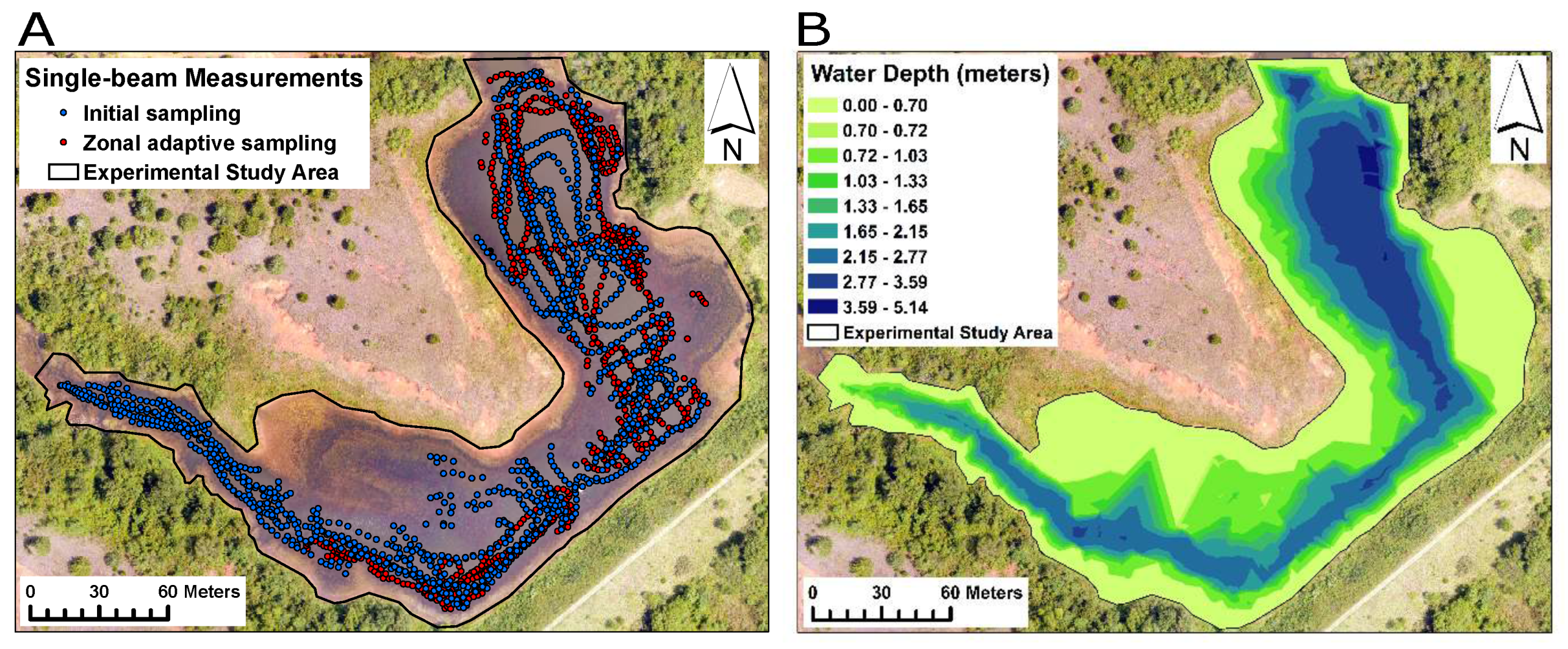
4.1. sUAS-Echosounder Measurements

The sUAS-echosounder dataset consisted of 2115 measurements, with 1212 of these collected from the initial set and 903 taken during the zonal-adaptive phase. Both initial (blue) and zonally-densified (red) points are displayed in Figure 3A. The single-beam echosounder estimated the depth to bed within the range of accuracy of the instrument (0.7 m ≤d < 80 m) with respect to the water elevation at the time of the measurements. Figure 3B shows a bathymetric map interpolated by employing a nearest neighbor technique, covering an area of 27,790 m 2 with a cell size of 1.26 m. The cell size was selected based on the mean distance between the echosounder measurements. The total estimated water volume is found to be 108,820 m 3 . The areas of the reservoir not detected by the echosounder (d < 0.7 m) are interpolated between 0 (shore) and 0.7 m, displayed in a uniform light-green color. The measured depths ( d 0.7 m) are shown in a green to blue gradient. Smooth transitions of water depths ranging from 2 m to 5.1 m are observed in the interpolated bathymetric map as a result of the dense preliminary and adaptive point sampling (Figure 3B), while depths between 0.7 m to 2 m are found to have larger depth variability. The lack of data on the shallower regions of the southwest caused abrupt transitions that the interpolation technique was unable to resolve (see Figure 3B).

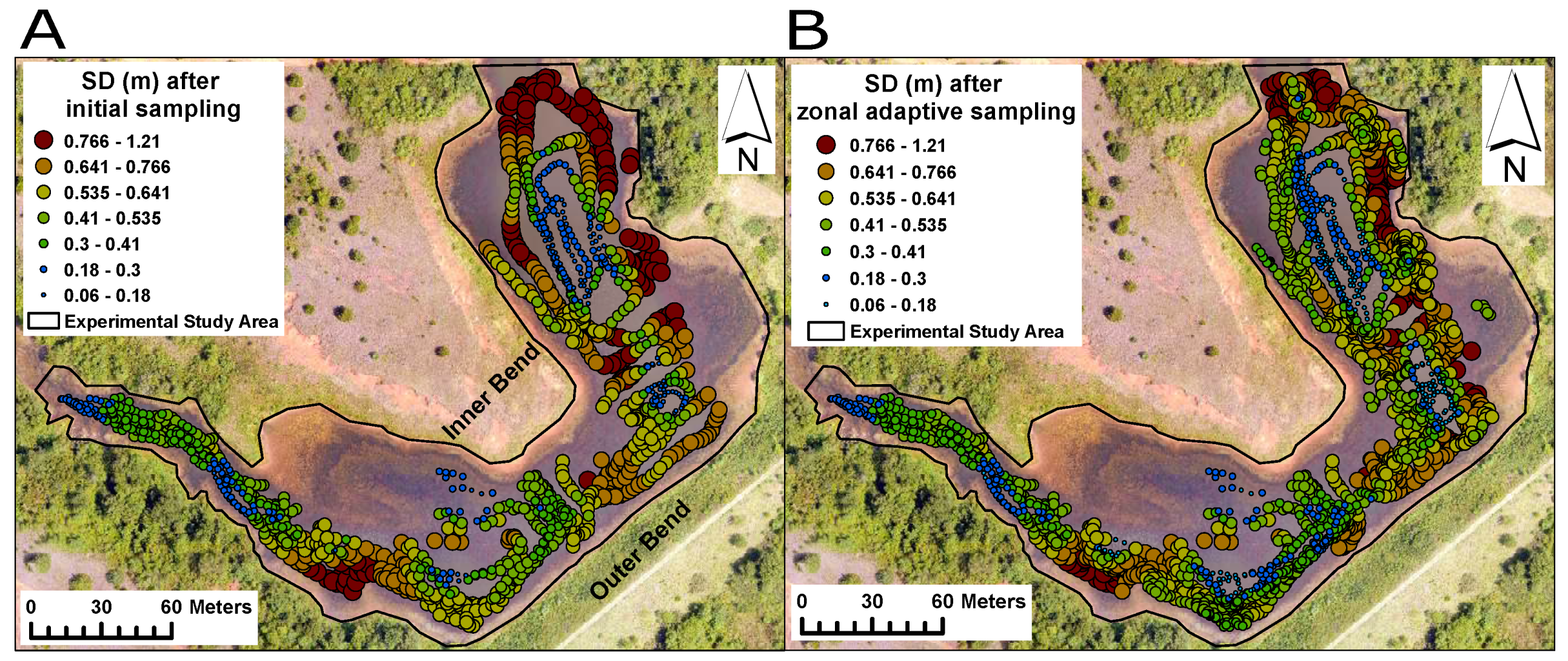
4.2. Zonal Adaptive Sampling

The spatial distribution of the clustered standard deviations from the preliminary and zonal adaptive samplings are shown in Figure 4A,B, respectively. In Figure 4A, the largest values of the standard deviation (i.e., 0.766 m to 1.21 m) are observed in the outside and inner bends of the northwest reservoir areas, as well as in a small region located in the southeast of the outer bend. The lowest values ranged between 0.06 and 0.18 m and were found within the deepest zones areas of the reservoir along the north and the southwest shores, which suggests a more homogeneous topography. The moderate standard deviation values (0.535 m to 0.641 m) are mostly found along the inner bend of the northern section of the reservoir (see Figure 4A). Before the adaptive sampling (Figure 4A), the number of high-standard deviation clusters (e.g., between 0.766 m and 1.21 m) appears to be larger than after the adaptive sampling (Figure 4B). This suggests that the homogeneity of the standard deviations values increased as a result of the adaptive strategy. A quantitative analysis reveals that, for the same pivots of the preliminary sampling, a re-calculation of the standard deviation results in reductions across all values, with up to 11.4 % reduction in its mean value with the largest improvements (18.1%) on the first quartile of the distribution. Table 1 summarizes the quartiles of the standard deviation for each stage of the sampling and its percent reduction for each quartile of the distribution. A small zone in the north of the reservoir was observed to remain constant in both sampling regimes. This is likely attributable to the inaccessibility to sample in private, neighboring lands where permissions to fly were not granted. The cluster analysis showed utility for the design of the zonal adaptive sampling and the newly added points improved the overall quality of the sampling procedure to capture bathymetric variability.

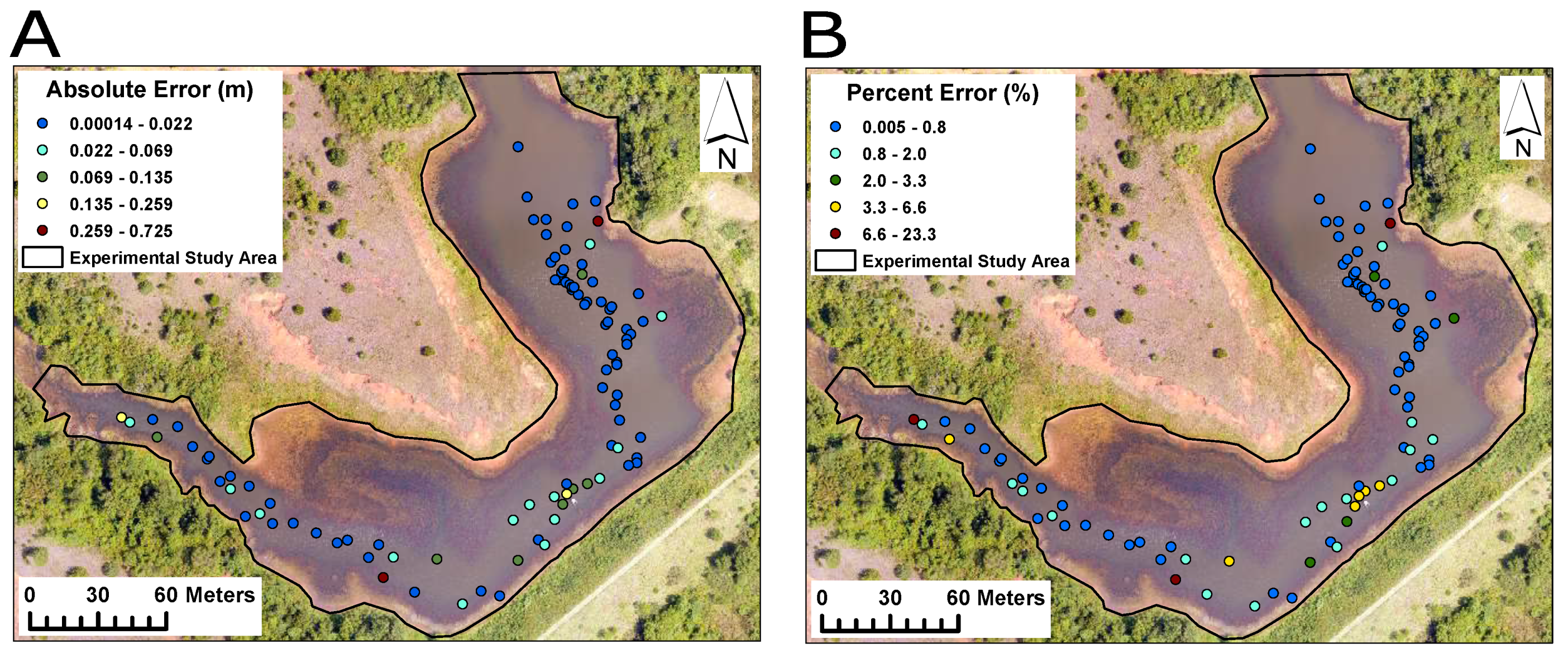
4.3. Echosounder Independent Validation

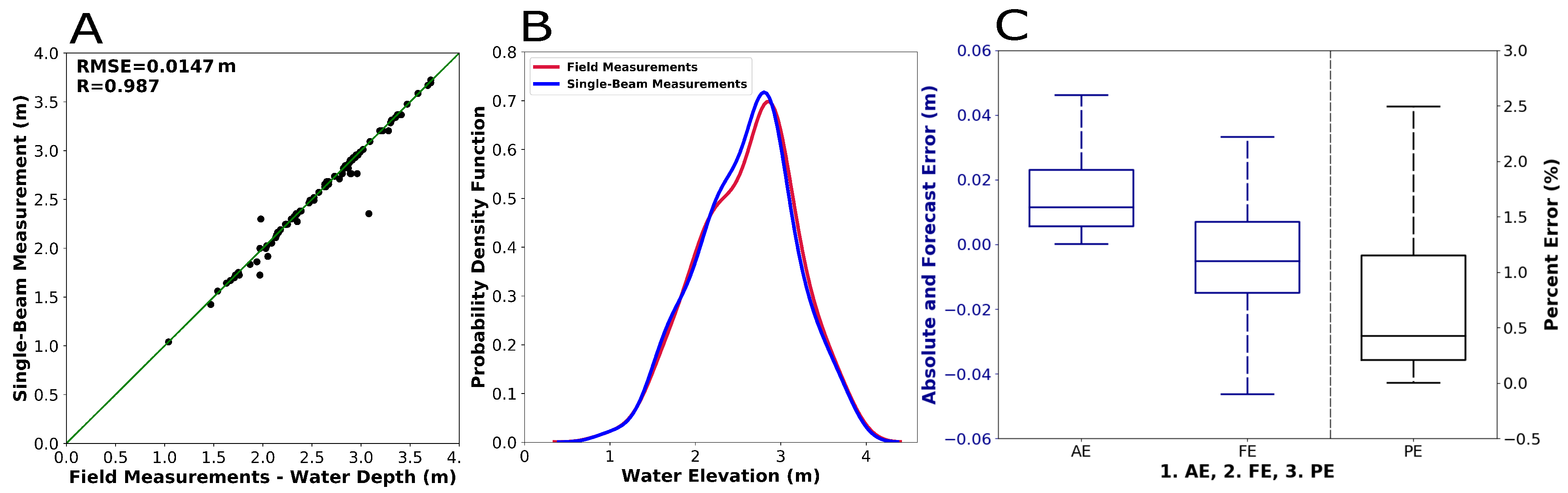
4.3.1. Scatterplot and Probability Density Functions

A scatterplot comparison between independent field observations (x-axis) and echosounder measurements (y-axis) is shown in Figure 5A with a green line depicting a perfect correlation between the field observations and the sonar-recorded measurements. A strong linear correlation between the field and echosounder measurements is made evident by the RMSE and R equal to 0.0147 m and 0.987. The majority of the single-beam measurements followed the green line, which shows a high accuracy. Some of the discrepancies between field and single-beam measurements may have been introduced by the manual rod observations due to the presence of unconsolidated, fine sediment at the bed or boat drift. A relatively good fit between the two probability density functions (field vs. echosounder) is observed (Figure 5B) and supported by the statistical similarities in distributional moments shown in Table 2. The mean of the field and single-beam measurements are equal to 2.7 m and 2.68 m, respectively; the variance is reported as 0.32 m (field measurements) and 0.47 m (single-beam measurements). Additionally, the probability density functions are both negatively skewed. Although the skewness indicates the largest difference between field observations with −0.26 and single-beam measurements −0.67, this skewness is hardly observed in Figure 5B.

4.3.2. Skill and Error Metrics

Echosounder measurements exhibited a good fit with field measurements as indicated by the statistical skill metrics shown in Figure 5 and Table 2. The correlation coefficient (R) was found to be equal to 0.987, indicating a high degree of data correspondence. Moreover, error metrics such as the RMSE (0.0147 m), MAE (0.03 m), MFE (0.02 m) and MAPE (1.39%) resulted in relatively small values (see Table 2). A positively skewed pattern was made evident in the box and whiskers distribution of the Absolute Error (AE), with values ranging from minimum 0 to maximum 0.73 m, and 75% of the data (3rd quartile) below 0.02% (see Figure 5C and Table 1). The median of the Forecasting Error (FE) distribution is found to be centered around the zero value (0.005 m) meaning that the single-beam measurements did not significantly under-estimate or over-estimate the values obtained by the field measurements (see Figure 5C and Table 2). Furthermore, the distribution of the percent error (PE) values ranged from 0.0005 to 23.5%, with 75% of the data (3rd quartile) less than 1.16% (see Figure 5C). This distribution was positively skewed with a heavy tail containing two outliers of 23.5% (see Table 2). These two outliers are located in shallow waters, below the range of accuracy of the single-beam (d < 0.7 m) (red points in Figure 6). Overall, the echosounder instrument showed good validation scores based on statistical skills and error metrics.
The spatial distribution of both AE and PE is shown in Figure 6A,B. AE has the lowest values, (blue points, Figure 6A) lying within the deepest zones of the reservoir on the northeast and southwest regions (see Figure 3B and Figure 6A), while larger values are observed in the south and southeast regions. There are two maximum values where AE equal to 0.73 m (red points in Figure 6A) that are located at places with depths of 1.5 and 3.5 m, as shown by Figure 5A. A similar pattern is shown from the spatial distribution of the PE (Figure 6B), where 75% of the values are below 1.16% and the two outliers of 23% match the location of the maximum AE (see Figure 6A,B and Table 2).
In general, the single-beam echosounder measurements showed centimeter-level accuracy when compared with the field measurements. Significant improvements are expected when UAS-SfM is merged with these echosounder measurements for a better representation of shallower areas (see Section 4.5). Merging of the two products should then be able to account for both deep and shallow water topography.

4.4. sUAS-SfM Accuracy

The location of the 60 ground checkpoints collected with a total station to assess the SfM accuracy is shown in Figure 7A. The distribution of the assessed elevations spans a broad range of topographic relief within the study area. This DEM has minimum and maximum elevations of 326 m and 358 m MSL, respectively (Figure 7B). A one-to-one scatterplot comparison between field and SfM data is shown in Figure 8, along with error and skill metrics. The correlation coefficient (R) value is equal to 0.993 and the RMSE and MAE values are equal to 0.37 m and 0.31 m correspondingly. Overall, the scatterplot and the skill and error metric results show a strong correlation between the ground checkpoints and the georeferenced DEM, which provide confidence in the accuracy of the applied sUAS-SfM technique.

4.5. sUAS-SfM Measurements

A high-resolution bathymetric map was constructed by subtracting a water elevation raster from the georeferenced DEM with a pixel resolution of 0.23 m to cover a total area of 27,790 m 2 . The apparent water depths were then multiplied by the refraction index. The results show that the depth and morphology of submerged areas are detected only when the reservoir bed is visible from the sUAS (see Figure 9). Noise created by beam reflection is introduced in some areas with a non-visible bed, as shown in Figure 7B and Figure 9. These results will complement the interpolated bathymetric map obtained with the sUAS-echosounder measurements (Section 4.6). The Pix4DMapper Pro® outputs of the SfM photogrammetry are found in the Supplementary Materials.

4.6. Merged sUAS-Echosounder and SfM Measurements

A hybrid bathymetric surveying resulted from merging the sUAS-echosounder and SfM techniques (Figure 10). The echosounder bathymetry (see Figure 3B) was implemented into this final interpolated raster as the main data source. The reservoir areas not surveyed by echosounder instrument were extracted from the sUAS-SfM measurements. The final product consists of a smooth raster covering an area 27,790 m 2 and total water volume of 106,892 m 3 . The water depths ranged from 0 to 5.11 m with the minimum depths detected from 0 to 0.05 m (see Figure 10). The final product kept the resolution of the coarser input raster, which corresponds to the sUAS-echosonder measurements. In general, the sUAS-SfM data successfully complemented the sUAS-echosounder survey as shown in Figure 10 when compared with Figure 3B.

5. Discussion and Future Work

In this study, the development of a novel technique consisting of utilizing sUAS imagery, echo soundings and adaptive sampling from autonomous systems, was presented along with its application for bathymetric surveying and estimation of reservoir storage. Mapping of submerged topography, by means of an sUAS, provides a low-cost, yet accurate alternative to submerged DEM construction when compared with conventional and emerging methods. Traditional techniques, such as, total-station surveying can only be employed in exposed terrain and shallow water systems, usually requires high investment of human power hours, and lacks the providing of robust data with high spatial resolution. On the other hand, multibeam echo sounding systems are considered an emerging technique broadly applied in oceanography. However, its use has been limited in the fields of terrestrial hydrology and geomorphology. Likewise, UAS imagery has been extensively applied to topography reconstruction, with little application to submerged areas.
Our research presents a cost-effective alternative to retrieve submerged topography in a reservoir, with a covered area of 27,790 m 2 , through a combination of echo sounding and SfM techniques within an adaptive sampling framework. The use of sUAS significantly reduced the time of data collection and human power hours, compared to traditional methods. For instance, the survey of this reservoir required approximately 15 h of fieldwork to collect the measurements with a team of two, a certified remote pilot in command and a skilled UAS operator. The zonal adaptive sampling also allowed an efficient and fast acquisition of data. The method is based on the outputs of a preliminary sampling to determine candidate areas for denser sampling according to the submerged terrain variability.
While the independent validation results are favorable, the quantitative assessment suggests that uncertainties in the manual level rod measurements by the presence of layers of unconsolidated, fine sediment can introduce disparities. These unconsolidated bed layers also impeded the wading for collection of field measurements in shallow zones unreachable by boat. For assuring the accuracy assessment on the sUAS imagery not validated with direct level rod measurements, a total station was used to georeference 294 images for precise representation of the terrain topography. As our capabilities advance, this georeferencing process may not be necessary in future research studies as Real Time Kinematic (RTK) GPS systems can be directly integrated into UAS conducting surveys. Another source of potential uncertainty was introduced by the horizontal and vertical GPS precision of the UAS as the coordinate location of the field measurements may not perfectly match with the echosounder data. Despite these issues, the bathymetric measurements compare favorably with the independent field observations.
Future steps can be focused in coupling zonal adaptive sampling with autonomous systems in a real-time self-correcting mode to learn and decide about density and speed of sampling at each step of the process. This real-time adaptive sampling could provide efficient data collection for applications involving very large data sets. Furthermore, our study suggests that bathymetry of water bodies can rapidly collect large data sets. Future endeavors could lead to the comparison of the efficiency, accuracy, spatial and temporal resolution of our method with respect to other remotely-based collection and more expensive technology (e.g., LiDAR and multi-beam echo soundings). As the capabilities of the centers for development of autonomous systems around the globe advance (e.g., CASS), more technology will be applied to earth surface science applications. For instance, future projects will aim to use adaptive sampling collected with miniaturized Real Time Kinematic (RTK) GPS units integrated with autonomous boats coupled to multibeam systems. Finally, this research can also be applied to fluvial systems and their modeling to construct the computational domains and validate hydrodynamic and turbulence resolving models.

6. Conclusions

In this study, we employed sUAS for determining submerged topography in a regional reservoir. A zonal adaptive sampling technique, adopted from the statistic and optimization fields, was implemented to improve the information quality. Thus, bathymetric changes were correctly captured. Results also showed that the standard deviation values within clusters of nearby points significantly decreased after the zonal adaptive sampling. A point-to-point validation was conducted to assess the ability of the echosounder to reproduce field measurements. The resulting scatterplot and probability density functions showed a good fit between the observed and echosounder measurements. Similarly, error and skill scores (i.e., MAE, MFE, RMSE, R and MAPE) showed a strong correlation between the tested instrument and field observations. sUAS imagery processed with SfM-photogrammetry was employed to quantify bathymetry in areas visible from the sUAS. A refraction correction was employed to account for the two-media problem. This sUAS-SfM technique was employed to complement the sUAS-echosounder measurements resulting in bathymetric surveying of the entire reservoir.
Overall, this research provides a novel approach that incorporates sUAS-echosounder and sUAS-SfM techniques to quantify bathymetry in water bodies. The submerged topography estimation capability of this low-cost and rapid method for large data set collection elucidates the possibility to apply it as a tool to further test a large variety of lakes and fluvial systems.

Supplementary Materials

The following are available online at https://www.mdpi.com/2072-4292/10/9/1362/s1. Pix4DMapper Pro® data outputs. This supplementary material has the purpose of reporting the Pix4DMapper Pro® outputs of the UAS SfM-photogrammetry. The UAS-imagery data were taken in August 2018 using the DJI Phantom 3 Pro. The outputs were processed in the professional drone mapping and photogrammetry software, Pix4DMapper Pro® in February 5th of 2018. The Pix4DMapper Pro® report is shown Table S1 and the statistics in Table S2. In summary, the Pix4DMapper Pro® outputs resulted in the following: (1) the area spanned was 0.276 km 2 ; (2) the dataset consisted of 294 images; (3) the mean projection error, in pixels, was equal to 0.255; and (4) the median of keypoints per images was 45,222. The mean absolute camera uncertainty values were found to be 0.15 m in the x and y directions and 0.374 m in the z direction.

Author Contributions

L.V.A., H.A.M. and P.B.C. conceived and designed the field campaigns and data acquisition; L.V.A. and H.A.M. led the field campaigns, and contributed to the data analysis and code developing; A.R.S. was in charge of deployments of the sUAS, and he also assisted with the SfM analysis; T.G.P. helped with building the geodatabase and figure editing; E.A.P.-L. assisted with a section writing and editing; L.V.A. led the paper writing and built the geodatabase.

Funding

This work was funded by the Center for Autonomous Sensing and Sampling (CASS), operated through the Office of the Vice President for Research at OU, Army Research Office project NO. W911NF-18-21-0007 and NSF EPSCoR RII Track II FEC Award Number: 1539070.

Acknowledgments

The authors thank Melissa Scott for providing undergraduate funds for the summer campaign of 2017 under the University of Oklahoma - NASA Space Grant Program. Summer field campaigns could not have been conducted without the help of the OU undergraduate student, Brandon Maples. We are also grateful to OU graduate student Brian R. Greene for serving as the remote pilot in command during the field campaigns.

Conflicts of Interest

The authors declare no conflict of interest. The funding sponsors had no role in the design of the study in the collection, analyses, or interpretation of data; in the writing of the manuscript, and in the decision to publish the results.

Appendix A. Statistical Metrics

The purpose of this appendix is to provide an interpretation and formulation of the skill and error metrics employed the echosounder independent validation (Section 4.3). Five metrics were used to validate the magnitude of the vector. These metrics are subdivided in two categories: absolute error metrics and one relative error metric. The absolute error metrics are: (1) Mean Absolute Error (MAE), (2) Mean Forecast Error (MFE), (3) Root Mean Square Error (RMSE) and (4) Pearson correlation coefficient (R). The relative error metric is: (5) Mean Absolute Percent Error (MAPE).
In the following paragraphs, the characteristics and formulation of these six metrics are presented:
(1)
Mean Absolute Error (MAE)
M A E = 100 n i = 1 n d ^ i d i ,
where: { d ^ i } is the water depth value of the echosounder measurements, { d i } is the field measurement, and {n} the number of data (same variables applied to all metrics).
The MAE measures the average of the error or differences between the echosounder and field measurements. The MAE is a linear metric where all the errors in the sample are weighted equally.
(2)
Mean Forecast Error (MFE)
M F E = 1 n i = 1 n d ^ i d i ,
The MFE is a measured the average differences between echosounder and field measurements. The ideal value for MFE is 0. Negative values of MFE means that the echosounder measurements tends to over-forecast and vice versa, positive MFE values the echosounder measurements tends to under-forecast.
(3)
Root Mean Square Error (RMSE)
R M S E = 1 n i = 1 n ( d ^ i d i ) 2 .
The RMSE represents the standard deviation of the differences between the echosounder and field measurements. This metric is nonlinear giving higher weight to large errors.
(4)
Pearson correlation coefficient (R)
R = i = 1 n ( d ^ i D ^ ¯ l ) ( d i D ¯ i ) i = 1 n ( d ^ i D ^ ¯ l ) 2 i = 1 n ( d ^ i D ¯ l ) 2 ,
where { D ^ ¯ l } is the mean of the echosounder measurements and { D ¯ l } is the mean of the field measurements.
The Pearson correlation coefficient (R) can range from −1 to 1. A value of 1 indicates a positive linear correlation between the echosounder and field measurements. A value of 0 indicates no linear correlation between echosounder and field measurements. A value of −1 indicates a negative correlation between the variables, meaning that echosounder measurements decrease while field measurements increase.
(5)
Mean Absolute Percent Error (MAPE)
M A P E = 100 n i = 1 n d ^ i d i d i .
The MAPE, also known as mean absolute percentage deviation (MAPD), is a simple metric where the difference between the echosounder and field measurements and divided by the field measurements and divided again by the number of points. The MAPE value is 0% for a perfect fit, but there is not upper limit restriction, and large values of MAPE are interpreted as large errors. Nonetheless, problems occur with small or close to zero denominators causing large MAPE values.

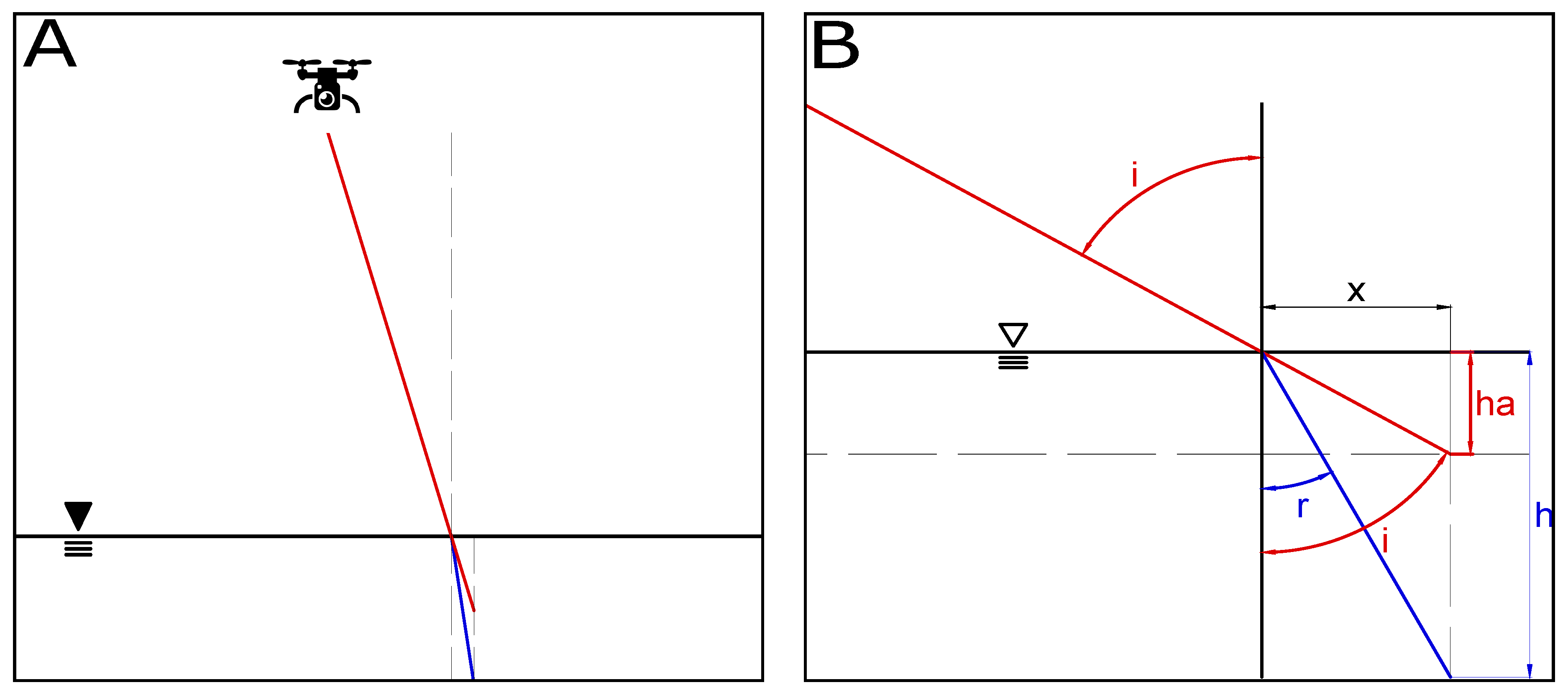
Appendix B. Snell–Descartes Law Simplification

A schematic representation and mathematical derivation are developed in this appendix to explain the Snell–Descartes law approximation for small angles, in terms of the actual and apparent depth of water. The results of this approximation have been applied to the SfM Post-Processing (Section 3.2.2) to improve the bathymetry retrievals from the sUAS-SfM technique.
  • Explanation of variables
  • i: Angle of incidence ( ),
  • r: Angle of refraction ( ),
  • x: Horizontal distance from where the light crosses the boundary between two media to where the light reaches the bottom of the lake (m),
  • n1: Index of refraction of air (∼1.0),
  • n2: Index of refraction of water (∼1.34),
  • h: Actual depth of water (m),
  • ha: Apparent depth of water (m).
The mathematical proof of the Snell–Descartes law aproximation based on Figure A1 is:
Figure A1. Schematic representation of the refraction of light at the interface between air and water, in terms of the depth (A) and apparent depth (B).
Remotesensing 10 01362 g0a1
t a n ( r ) = x h h = x t a n ( r )
and:
t a n ( i ) = x h a h a = x t a n ( i ) .
Hence:
h h a = t a n ( i ) t a n ( r ) .
The small-angle approximation is applied, when the angle approaches zero, which is predominantly true for this case, since the UAS image collection was obtained at Nadir. Thus, Equation (A8) is equal to:
t a n ( i ) t a n ( r ) s i n ( i ) s i n ( r ) = n 2 n 1 .
Therefore,
s i n ( r ) s i n ( i ) = n 2 n 1 = h h a .
Since n 1 is equal to 1 and n 2 is equal to 1.34, the final result becomes:
h = 1.34 h a .

References

  1. Legleiter, C.J. Remote measurement of river morphology via fusion of LiDAR topography and spectrally based bathymetry: Measuring river morphology with LiDAR and spectral bathymetry. Earth Surf. Process. Landf. 2012, 37, 499–518. [Google Scholar] [CrossRef]
  2. Niethammer, U.; James, M.; Rothmund, S.; Travelletti, J.; Joswig, M. UAV-based remote sensing of the Super-Sauze landslide: Evaluation and results. Eng. Geol. 2012, 128, 2–11. [Google Scholar] [CrossRef]
  3. Passalacqua, P.; Belmont, P.; Staley, D.M.; Simley, J.D.; Arrowsmith, J.R.; Bode, C.A.; Crosby, C.; DeLong, S.B.; Glenn, N.F.; Kelly, S.A.; et al. Analyzing high resolution topography for advancing the understanding of mass and energy transfer through landscapes: A review. Earth Sci. Rev. 2015, 148, 174–193. [Google Scholar] [CrossRef] [Green Version]
  4. Tsai, Z.X.; You, G.J.Y.; Lee, H.Y.; Chiu, Y.J. Use of a total station to monitor post-failure sediment yields in landslide sites of the Shihmen reservoir watershed, Taiwan. Geomorphology 2012, 139–140, 438–451. [Google Scholar] [CrossRef]
  5. Wheaton, J.M.; Brasington, J.; Darby, S.E.; Sear, D.A. Accounting for uncertainty in DEMs from repeat topographic surveys: Improved sediment budgets. Earth Surf. Process. Landf. 2010, 35, 136–156. [Google Scholar] [CrossRef]
  6. Alvarez, L.V. Turbulence, Sediment Transport, Erosion, and Sandbar Beach Failure Processes in Grand Canyon. Ph.D. Thesis, Arizona State University, Tempe, AZ, USA, 2015. [Google Scholar]
  7. Alvarez, L.V.; Schmeeckle, M.W.; Grams, P.E. A detached eddy simulation model for the study of lateral separation zones along a large canyon-bound river. J. Geophys. Res. 2017, 122, 25–49. [Google Scholar] [CrossRef]
  8. Moreno, H.A.; Gupta, H.V.; White, D.D.; Sampson, D.A. Modeling the distributed effects of forest thinning on the long-term water balance and streamflow extremes for a semi-arid basin in the southwestern US. Hydrol. Earth Syst. Sci. 2016, 20, 1241–1267. [Google Scholar] [CrossRef] [Green Version]
  9. Moreno, H.A.; Vivoni, E.R.; Gochis, D.J. Addressing uncertainty in reflectivity-rainfall relations in mountain watersheds during summer convection. Hydrol. Process. 2014, 28, 688–704. [Google Scholar] [CrossRef]
  10. Moreno, H.A.; Vivoni, E.R.; Gochis, D.J. Utility of Quantitative Precipitation Estimates for high resolution hydrologic forecasts in mountain watersheds of the Colorado Front Range. J. Hydrol. 2012, 438–439, 66–83. [Google Scholar] [CrossRef]
  11. Moreno, H.A.; Vivoni, E.R.; Gochis, D.J. Limits to Flood Forecasting in the Colorado Front Range for Two Summer Convection Periods Using Radar Nowcasting and a Distributed Hydrologic Model. J. Hydrol. 2013, 14, 1075–1097. [Google Scholar] [CrossRef]
  12. Alvarez, L.V.; Schmeeckle, M.W. Erosion of river sandbars by diurnal stage fluctuations in the Colorado River in the Marble and Grand Canyons: Full-scaled laboratory experiments. River Res. Appl. 2013, 29, 839–854. [Google Scholar] [CrossRef]
  13. Converse, Y.K.; Hawkins, C.P.; Valdez, R.A. Habitat relationships of subadult humpback chub in the Colorado River through Grand Canyon: Spatial variability and implications of flow regulation. Regul. River 1998, 14, 267–284. [Google Scholar] [CrossRef]
  14. Gerig, B.; Dodrill, M.J.; Pine, W.E. Habitat Selection and Movement of Adult Humpback Chub in the Colorado River in Grand Canyon, Arizona, during an Experimental Steady Flow Release. N. J. Fish. Manag. 2014, 34, 39–48. [Google Scholar] [CrossRef]
  15. Korman, J.; Wiele, S.M.; Torizzo, M. Modelling effects of discharge on habitat quality and dispersal of juvenile humpback chub (Gila cypha) in the Colorado River, Grand Canyon. River Res. Appl. 2004, 20, 379–400. [Google Scholar] [CrossRef]
  16. Orr, H.; Large, A.; Newson, M.; Walsh, C. A predictive typology for characterising hydromorphology. Geomorphology 2008, 100, 32–40. [Google Scholar] [CrossRef]
  17. Wilson, M.F.J.; O’Connell, B.; Brown, C.; Guinan, J.C.; Grehan, A.J. Multiscale Terrain Analysis of Multibeam Bathymetry Data for Habitat Mapping on the Continental Slope. Mar. Geodesy 2007, 30, 3–35. [Google Scholar] [CrossRef] [Green Version]
  18. Keim, R.F.; Skaugset, A.E.; Bateman, D.S. Digital terrain modeling of small stream channels with a total-station theodolite. Adv. Water Resour. 1999, 23, 41–48. [Google Scholar] [CrossRef]
  19. Carbonneau, P.E.; Lane, S.N.; Bergeron, N.E. Cost-effective non-metric close-range digital photogrammetry and its application to a study of coarse gravel river beds. Int. J. Remote Sens. 2003, 24, 2837–2854. [Google Scholar] [CrossRef]
  20. Fryer, J.G.; Kniest, H.T. Errors in depth determination caused by waves in through-water photogrammetry. Photogramm. Rec. 1985, 11, 745–753. [Google Scholar] [CrossRef]
  21. Lane, S.N. The measurement of river channel morphology using digital photogrammetry. Photogramm. Rec. 2000, 16, 937–961. [Google Scholar] [CrossRef]
  22. Westaway, R.M.; Lane, S.N.; Hicks, D.M. Remote survey of large-scale braided, gravel-bed rivers using digital photogrammetry and image analysis. Int. J. Remote Sens. 2003, 24, 795–815. [Google Scholar] [CrossRef]
  23. Westaway, R.M.; Lane, S.N.; Hicks, D.M. Remote sensing of clear-water, shallow, gravel-bed rivers using digital photogrammetry. Photogramm. Eng. Remote Sens. 2001, 67, 1271–1282. [Google Scholar]
  24. Bailly, J.S.; Kinzel, P.J.; Allouis, T.; Feurer, D.; Le Coarer, Y. Airborne LiDAR Methods Applied to Riverine Environments. In Fluvial Remote Sensing for Science and Management; John Wiley & Sons, Ltd.: Hoboken, NJ, USA, 2012; pp. 141–161. [Google Scholar]
  25. Brock, J.C.; Purkis, S.J. The Emerging Role of Lidar Remote Sensing in Coastal Research and Resource Management. J. Coast. Res. 2009, 10053, 1–5. [Google Scholar] [CrossRef]
  26. Kinzel, P.J.; Legleiter, C.J.; Nelson, J.M. Mapping river bathymetry with a small footprint green LiDAR: Applications and challenges. J. Am. Water Resour. Assoc. 2013, 49, 183–204. [Google Scholar] [CrossRef]
  27. Hilldale, R.C.; Raff, D. Assessing the ability of airborne LiDAR to map river bathymetry. Earth Surf. Process. Landf. 2008, 33, 773–783. [Google Scholar] [CrossRef]
  28. McKean, J.; Nagel, D.; Tonina, D.; Bailey, P.; Wright, C.W.; Bohn, C.; Nayegandhi, A. Remote Sensing of Channels and Riparian Zones with a Narrow-Beam Aquatic-Terrestrial LIDAR. Remote Sens. 2009, 1, 1065–1096. [Google Scholar] [CrossRef] [Green Version]
  29. Fonstad, M.A.; Dietrich, J.T.; Courville, B.C.; Jensen, J.L.; Carbonneau, P.E. Topographic structure from motion: A new development in photogrammetric measurement. Earth Surf. Process. Landf. 2013, 38, 421–430. [Google Scholar] [CrossRef]
  30. Lejot, J.; Delacourt, C.; Piégay, H.; Fournier, T.; Trémélo, M.L.; Allemand, P. Very high spatial resolution imagery for channel bathymetry and topography from an unmanned mapping controlled platform. Earth Surf. Process. Landf. 2007, 32, 1705–1725. [Google Scholar] [CrossRef]
  31. Marcus, W.A.; Fonstad, M.A. Optical remote mapping of rivers at sub-meter resolutions and watershed extents. Earth Surf. Process. Landf. 2008, 33, 4–24. [Google Scholar] [CrossRef]
  32. Clapuyt, F.; Vanacker, V.; Van Oost, K. Reproducibility of UAV-based earth topography reconstructions based on Structure-from-Motion algorithms. Geomorphology 2016, 260, 4–15. [Google Scholar] [CrossRef]
  33. Dunford, R.; Michel, K.; Gagnage, M.; Piégay, H.; Trémelo, M.L. Potential and constraints of Unmanned Aerial Vehicle technology for the characterization of Mediterranean riparian forest. Int. J. Remote Sens. 2009, 30, 4915–4935. [Google Scholar] [CrossRef]
  34. Harwin, S.; Lucieer, A. Assessing the Accuracy of Georeferenced Point Clouds Produced via Multi-View Stereopsis from Unmanned Aerial Vehicle (UAV) Imagery. Remote Sens. 2012, 4, 1573–1599. [Google Scholar] [CrossRef] [Green Version]
  35. Smith, M.; Carrivick, J.; Quincey, D. Structure from motion photogrammetry in physical geography. Prog. Phys. Geogr. 2016, 40, 247–275. [Google Scholar] [CrossRef]
  36. Turner, D.; Lucieer, A.; Watson, C. An Automated Technique for Generating Georectified Mosaics from Ultra-High Resolution Unmanned Aerial Vehicle (UAV) Imagery, Based on Structure from Motion (SfM) Point Clouds. Remote Sens. 2012, 4, 1392–1410. [Google Scholar] [CrossRef] [Green Version]
  37. Woodget, A.S.; Carbonneau, P.E.; Visser, F.; Maddock, I.P. Quantifying submerged fluvial topography using hyperspatial resolution UAS imagery and structure from motion photogrammetry: Submerged fluvial topography from UAS imagery and SfM. Earth Surf. Process. Landf. 2015, 40, 47–64. [Google Scholar] [CrossRef]
  38. Hugenholtz, C.H.; Whitehead, K.; Brown, O.W.; Barchyn, T.E.; Moorman, B.J.; LeClair, A.; Riddell, K.; Hamilton, T. Geomorphological mapping with a small unmanned aircraft system (sUAS): Feature detection and accuracy assessment of a photogrammetrically-derived digital terrain model. Geomorphology 2013, 194, 16–24. [Google Scholar] [CrossRef] [Green Version]
  39. Jaakkola, A.; Hyyppä, J.; Kukko, A.; Yu, X.; Kaartinen, H.; Lehtomäki, M.; Lin, Y. A low-cost multi-sensoral mobile mapping system and its feasibility for tree measurements. ISPRS J. Photogramm. Remote Sens. 2010, 65, 514–522. [Google Scholar] [CrossRef]
  40. Tarolli, P. High-resolution topography for understanding Earth surface processes: Opportunities and challenges. Geomorphology 2014, 216, 295–312. [Google Scholar] [CrossRef]
  41. Watts, A.C.; Ambrosia, V.G.; Hinkley, E.A. Unmanned Aircraft Systems in Remote Sensing and Scientific Research: Classification and Considerations of Use. Remote Sens. 2012, 4, 1671–1692. [Google Scholar] [CrossRef] [Green Version]
  42. Javernick, L.; Brasington, J.; Caruso, B. Modeling the topography of shallow braided rivers using Structure-from-Motion photogrammetry. Geomorphology 2014, 213, 166–182. [Google Scholar] [CrossRef]
  43. Rosnell, T.; Honkavaara, E. Point Cloud Generation from Aerial Image Data Acquired by a Quadrocopter Type Micro Unmanned Aerial Vehicle and a Digital Still Camera. Sensors 2012, 12, 453–480. [Google Scholar] [CrossRef] [PubMed] [Green Version]
  44. Verhoeven, G.; Doneus, M.; Briese, C.; Vermeulen, F. Mapping by matching: A computer vision-based approach to fast and accurate georeferencing of archaeological aerial photographs. J. Archaeol. Sci. 2012, 39, 2060–2070. [Google Scholar] [CrossRef]
  45. Vericat, D.; Brasington, J.; Wheaton, J.; Cowie, M. Accuracy assessment of aerial photographs acquired using lighter-than-air blimps: Low-cost tools for mapping river corridors. River Res. Appl. 2009, 25, 985–1000. [Google Scholar] [CrossRef]
  46. MacVicar, B.; Piegay, H.; Henderson, A.; Comiti, F.; Oberlin, C.; Pecorari, E. Quantifying the temporal dynamics of wood in large rivers: Field trials of wood surveying, dating, tracking, and monitoring techniques. Earth Surf. Process. Landf. 2009, 34, 2031–2046. [Google Scholar] [CrossRef]
  47. Smith, M.J.; Chandler, J.; Rose, J. High spatial resolution data acquisition for the geosciences: Kite aerial photography. Earth Surf. Process. Landf. 2009, 34, 155–161. [Google Scholar] [CrossRef]
  48. Hervouet, A.; Dunford, R.; Piégay, H.; Belletti, B.; Trémélo, M.L. Analysis of Post-flood Recruitment Patterns in Braided-Channel Rivers at Multiple Scales Based on an Image Series Collected by Unmanned Aerial Vehicles, Ultra-light Aerial Vehicles, and Satellites. GISci. Remote Sens. 2011, 48, 50–73. [Google Scholar] [CrossRef]
  49. Dietrich, J.T. Bathymetric Structure-from-Motion: Extracting shallow stream bathymetry from multi-view stereo photogrammetry. Earth Surf. Process. Landf. 2017, 42, 355–364. [Google Scholar] [CrossRef]
  50. Cartwright, D.S.; Clarke, J.H. Multibeam surveys of the frazer river delta, coping with an extreme refraction environment. In Proceedings of the 2002 Canadian Hydrographic Conference, Toronto, ON, Canada, 28–31 May 2002. [Google Scholar]
  51. Clarke, J.E.H.; Mayer, L.A.; Wells, D.E. Shallow-water imaging multibeam sonars: a new tool for investigating seafloor processes in the coastal zone and on the continental shelf. Mar. Geophys. Res. 1996, 18, 607–629. [Google Scholar] [CrossRef]
  52. Dinehart, R.L. Bedform movement recorded by sequential single-beam surveys in tidal rivers. J. Hydrol. 2002, 258, 25–39. [Google Scholar] [CrossRef]
  53. Gerlotto, F.; Soria, M.; Fréon, P. From two dimensions to three: The use of multibeam sonar for a new approach in fisheries acoustics. Can. J. Fish. Aquat. 1999, 56, 6–12. [Google Scholar] [CrossRef]
  54. Guerrero, M.; Lamberti, A. Flow Field and Morphology Mapping Using ADCP and Multibeam Techniques: Survey in the Po River. J. Hydraul. Res. 2011, 137, 1576–1587. [Google Scholar] [CrossRef]
  55. Muste, M.; Baranya, S.; Tsubaki, R.; Kim, D.; Ho, H.; Tsai, H.; Law, D. Acoustic mapping velocimetry. Water Resour. Res. 2016, 52, 4132–4150. [Google Scholar] [CrossRef] [Green Version]
  56. Parsons, D.R.; Best, J.L.; Orfeo, O.; Hardy, R.J.; Kostaschuk, R.; Lane, S.N. Morphology and flow fields of three-dimensional dunes, Rio Paraná, Argentina: Results from simultaneous multibeam echo sounding and acoustic Doppler current profiling: Three dimensional alluvial dunes, Rio Parana. J. Geophys. Res 2005, 110. [Google Scholar] [CrossRef]
  57. Somoza, L. Seabed morphology and hydrocarbon seepage in the Gulf of Cádiz mud volcano area: Acoustic imagery, multibeam and ultra-high resolution seismic data. Mar. Geol. 2003, 195, 153–176. [Google Scholar] [CrossRef]
  58. Fonseca, L.; Mayer, L. Remote estimation of surficial seafloor properties through the application Angular Range Analysis to multibeam sonar data. Mar. Geophys. Res. 2007, 28, 119–126. [Google Scholar] [CrossRef]
  59. Dinehart, R.L.; Burau, J.R. Averaged indicators of secondary flow in repeated acoustic Doppler current profiler crossings of bends: Averaged indicators of secondary flow. Water Resour. Res. 2005, 41. [Google Scholar] [CrossRef]
  60. Muste, M.; Baranya, S.; Tsubaki, R.; Kim, D.; Ho, H.C.; Tsai, H.W.; Law, D. Acoustic Mapping Velocimetry proof-of-concept experiment. In Proceedings of the 36th IAHR World Congress, The Hague, The Netherlands, 28 June–3 July 2015. [Google Scholar]
  61. Venditti, J.G.; Rennie, C.D.; Bomhof, J.; Bradley, R.W.; Little, M.; Church, M. Flow in bedrock canyons. Nature 2014, 513, 534–537. [Google Scholar] [CrossRef] [PubMed]
  62. Viney, I.T.; Kirk, G.R. Remote Control and Viewing for A Total Station. Google Patents 6,034.722, 7 March 2000. [Google Scholar]
  63. Cross, E.; Koo, K.; Brownjohn, J.; Worden, K. Long-term monitoring and data analysis of the Tamar Bridge. Mech. Syst. Signal. Process. 2013, 35, 16–34. [Google Scholar] [CrossRef] [Green Version]
  64. Ehrhart, M.; Lienhart, W. Monitoring of civil engineering structures using a state-of-the-art image assisted total station. J. Appl. Geodesy 2015, 9, 174–182. [Google Scholar] [CrossRef]
  65. Mill, T.; Alt, A.; Liias, R. Combined 3D building surveying techniques—Terrestrial laser scanning (TLS) and total station surveying for BIM data management purposes. J. Civ. Eng. Manag. 2013, 19, S23–S32. [Google Scholar] [CrossRef]
  66. Psimoulis, P.A.; Stiros, S.C. Measuring Deflections of a Short-Span Railway Bridge Using a Robotic Total Station. J. Bridge Eng. 2013, 18, 182–185. [Google Scholar] [CrossRef]
  67. Henry, E.; Mayer, C.; Rott, H. Mapping mining-induced subsidence from space in a hard rock mine: Example of SAR interferometry application at Kiruna mine. CIM Bull. 2004, 97, 1–5. [Google Scholar]
  68. Hürkamp, K.; Raab, T.; Völkel, J. Two and three-dimensional quantification of lead contamination in alluvial soils of a historic mining area using field portable X-ray fluorescence (FPXRF) analysis. Geomorphology 2009, 110, 28–36. [Google Scholar] [CrossRef]
  69. Nainwal, H.; Negi, B.; Chaudhary, M.; Sajwan, K.; Gaurav, A. Temporal changes in rate of recession: Evidences from Satopanth and Bhagirath Kharak glaciers, Uttarakhand, using Total Station Survey. Curr. Sci. 2008, 94, 653–660. [Google Scholar]
  70. Smith, M.; Vericat, D. Evaluating shallow-water bathymetry from through-water terrestrial laser scanning under a range of hydraulic and physical water quality conditions. River Res. Appl. 2014, 30, 905–924. [Google Scholar] [CrossRef]
  71. Chen, X.; Vierling, L.; Rowell, E.; DeFelice, T. Using lidar and effective LAI data to evaluate IKONOS and Landsat 7 ETM+ vegetation cover estimates in a ponderosa pine forest. Remote Sens. Environ. 2004, 91, 14–26. [Google Scholar] [CrossRef]
  72. Genç, L.; Dewitt, B.; Smith, S. Determination of wetland vegetation height with LIDAR. Turk. J. Agric. For. 2004, 28, 63–71. [Google Scholar]
  73. Saito, Y.; Kanoh, M.; Hatake, K.I.; Kawahara, T.D.; Nomura, A. Investigation of laser-induced fluorescence of several natural leaves for application to lidar vegetation monitoring. Appl. Opt. 1998, 37, 431–437. [Google Scholar] [CrossRef] [PubMed]
  74. Hudak, A.T.; Lefsky, M.A.; Cohen, W.B.; Berterretche, M. Integration of lidar and Landsat ETM+ data for estimating and mapping forest canopy height. Remote Sens. Environ. 2002, 82, 397–416. [Google Scholar] [CrossRef] [Green Version]
  75. Reutebuch, S.E.; McGaughey, R.J.; Andersen, H.E.; Carson, W.W. Accuracy of a high-resolution lidar terrain model under a conifer forest canopy. Can. J. Remote Sens. 2003, 29, 527–535. [Google Scholar] [CrossRef] [Green Version]
  76. Simard, M.; Pinto, N.; Fisher, J.B.; Baccini, A. Mapping forest canopy height globally with spaceborne lidar. J. Geophys. Res. 2011, 116. [Google Scholar] [CrossRef]
  77. Andersen, H.E.; McGaughey, R.J.; Reutebuch, S.E. Estimating forest canopy fuel parameters using LIDAR data. Remote Sens. Environ. 2005, 94, 441–449. [Google Scholar] [CrossRef]
  78. Clark, M.L.; Clark, D.B.; Roberts, D.A. Small-footprint lidar estimation of sub-canopy elevation and tree height in a tropical rain forest landscape. Remote Sens. Environ. 2004, 91, 68–89. [Google Scholar] [CrossRef]
  79. Kwak, D.A.; Lee, W.K.; Lee, J.H.; Biging, G.S.; Gong, P. Detection of individual trees and estimation of tree height using LiDAR data. J. For. Res. 2007, 12, 425–434. [Google Scholar] [CrossRef]
  80. Chehata, N.; Guo, L.; Mallet, C. Airborne LiDAR feature selection for urban classification using random forests. Int. Arch. Photogramm. Remote Sens. Spat. Inf. Sci. 2009, 38, W8. [Google Scholar]
  81. Guo, L.; Chehata, N.; Mallet, C.; Boukir, S. Relevance of airborne lidar and multispectral image data for urban scene classification using Random Forests. J. Photogramm. Remote Sens. 2011, 66, 56–66. [Google Scholar] [CrossRef]
  82. Mallet, C.; Bretar, F.; Roux, M.; Soergel, U.; Heipke, C. Relevance assessment of full-waveform lidar data for urban area classification. ISPRS J. Photogramm. Remote Sens. 2011, 66, S71–S84. [Google Scholar] [CrossRef]
  83. Bangen, S.G.; Wheaton, J.M.; Bouwes, N.; Bouwes, B.; Jordan, C. A methodological intercomparison of topographic survey techniques for characterizing wadeable streams and rivers. Geomorphology 2014, 206, 343–361. [Google Scholar] [CrossRef]
  84. Feurer, D.; Bailly, J.S.; Puech, C.; Le Coarer, Y.; Viau, A.A. Very-high-resolution mapping of river-immersed topography by remote sensing. Prog. Phys. Geogr. 2008, 32, 403–419. [Google Scholar] [CrossRef]
  85. Kinzel, P.J. Advanced tools for river science: EAARL and MD_SWMS. In PNMAP Special Publication: Remote Sensing Applications for Aquatic Resources Monitoring. Pacific Northwest Aquatic Monitoring Partnership; PNMAP: Bangkok, Thailand, 2009; pp. 17–26. [Google Scholar]
  86. Brock, J.C.; Wright, C.W.; Patterson, M.; Nayegandhi, A.; Patterson, J.; Harris, M.S.; Mosher, L. EAARL Submarine Topography: Biscayne National Park; Technical Report; US Geological Survey: Reston, VA, USA, 2006.
  87. Irish, J.L.; Lillycrop, W.J. Scanning laser mapping of the coastal zone: The SHOALS system. ISPRS J. Photogramm. Remote Sens. 1999, 54, 123–129. [Google Scholar] [CrossRef]
  88. Bonisteel, J.M.; Nayegandhi, A.; Wright, C.W.; Brock, J.C.; Nagle, D. Experimental Advanced Airborne Research LiDAR (EAARL) Data Processing Manual; Technical Report; US Geological Survey: Reston, VA, USA, 2009.
  89. Nayegandhi, A.; Brock, J.C.; Wright, C.W. Classifying vegetation using NASA’s Experimental Advanced Airborne Research Lidar (EAARL) at Assateague Island National Seashore. In Proceedings of the 2005 ASPRS Annual Conference, Baltimore, MA, USA, 7–11 March 2005. [Google Scholar]
  90. Skinner, K.D. Evaluation of LiDAR-Acquired Bathymetric and Topographic Data Accuracy in Various Hydrogeomorphic Settings in the Deadwood and South Fork Boise Rivers, West-Central Idaho, 2007; Technical Report; US Geological Survey: Reston, VA, USA, 2011.
  91. Wright, C.W.; Troche, R.J.; Kranenburg, C.J.; Klipp, E.S.; Fredericks, X.; Nagle, D.B. EAARL-B Submerged Topography: Barnegat Bay, New Jersey, Post-Hurricane Sandy, 2012–2013; Technical Report; US Geological Survey: Reston, VA, USA, 2014.
  92. Wright, C.W.; Fredericks, X.; Troche, R.J.; Klipp, E.S.; Kranenburg, C.J.; Nagle, D.B. EAARL-B Coastal Topography: Eastern New Jersey, Hurricane Sandy, 2012: First Surface; Technical Report Data Series 885; US Geological Survey: Reston, VA, USA, 2014.
  93. Kostylev, V.E.; Todd, B.J.; Fader, G.B.; Courtney, R.C.; Cameron, G.D.; Pickrill, R.A. Benthic habitat mapping on the Scotian Shelf based on multibeam bathymetry, surficial geology and sea floor photographs. Mar. Ecol. Prog. Ser. 2001, 219, 121–137. [Google Scholar] [CrossRef] [Green Version]
  94. Kaplinski, M.; Hazel, J.E., Jr.; Grams, P.E.; Kohl, K.; Buscombe, D.D.; Tusso, R.B. Channel Mapping River Miles 29–62 of the Colorado River in Grand Canyon National Park, Arizona, May 2009; Technical Report No. 2017-1030; US Geological Survey: Reston, VA, USA, 2017.
  95. Maxwell, S.L.; Smith, A.V. Generating River Bottom Profiles with a Dual-Frequency Identification Sonar (DIDSON). N. J. Fish. Manag. 2007, 27, 1294–1309. [Google Scholar] [CrossRef]
  96. Ashworth, P.J.; Best, J.L.; Roden, J.E.; Bristow, C.S.; Klaassen, G.J. Morphological evolution and dynamics of a large, sand braid-bar, Jamuna River, Bangladesh. Sedimentology 2000, 47, 533–555. [Google Scholar] [CrossRef]
  97. Harbor, D.J. Dynamics of bedforms in the lower Mississippi River. J. Sediment. Res. 1998, 68, 750–762. [Google Scholar] [CrossRef]
  98. Lewin, J.; Weir, M.J.C. Morphology and recent history of the lower Spey. Scott. Geogr. Mag. 1977, 93, 45–51. [Google Scholar] [CrossRef]
  99. Lewin, J.; Manton, M. Welsh floodplain studies: The nature of floodplain geometry. J. Hydrol. 1975, 25, 37–50. [Google Scholar] [CrossRef]
  100. Mertes, L.A. Remote sensing of riverine landscapes. Freshwater Biol. 2002, 47, 799–816. [Google Scholar] [CrossRef]
  101. Lapointe, M.F.; Secretan, Y.; Driscoll, S.N.; Bergeron, N.; Leclerc, M. Response of the Ha! Ha! River to the flood of July 1996 in the Saguenay region of Quebec: Large-scale avulsion in a glaciated valley. Water Resour. Res. 1998, 34, 2383–2392. [Google Scholar] [CrossRef] [Green Version]
  102. Lane, S.N. The reconstruction of bed material yield and supply histories in gravel-bed streams. Catena 1997, 30, 183–196. [Google Scholar] [CrossRef]
  103. Lane, S.N.; Richards, K.S.; Chandler, J.H. Morphological Estimation of the Time-Integrated Bed Load Transport Rate. Water Resour. Res. 1995, 31, 761–772. [Google Scholar] [CrossRef]
  104. Nikora, V.I.; Goring, D.G.; Biggs, B.J.F. On gravel-bed roughness characterization. Water Resour. Res. 1998, 34, 517–527. [Google Scholar] [CrossRef] [Green Version]
  105. Bendig, J.; Willkomm, M.; Tilly, N.; Gnyp, M.L.; Bennertz, S.; Qiang, C.; Miao, Y.; Lenz-Wiedemann, V.I.S.; Bareth, G. Very high resolution crop surface models (CSMs) from UAV-based stereo images for rice growth monitoring in Northeast China. Int. Arch. Photogramm. Remote Sens. Spat. Inf. Sci 2013, 40, 45–50. [Google Scholar] [CrossRef]
  106. Dandois, J.P.; Ellis, E.C. Remote Sensing of Vegetation Structure Using Computer Vision. Remote Sens. 2010, 2, 1157–1176. [Google Scholar] [CrossRef] [Green Version]
  107. James, M.R.; Robson, S. Straightforward reconstruction of 3D surfaces and topography with a camera: Accuracy and geoscience application. J. Geophys. Res 2012, 117, F03017. [Google Scholar] [CrossRef]
  108. Mancini, F.; Dubbini, M.; Gattelli, M.; Stecchi, F.; Fabbri, S.; Gabbianelli, G. Using Unmanned Aerial Vehicles (UAV) for High-Resolution Reconstruction of Topography: The Structure from Motion Approach on Coastal Environments. Remote Sens. 2013, 5, 6880–6898. [Google Scholar] [CrossRef] [Green Version]
  109. Westoby, M.; Brasington, J.; Glasser, N.; Hambrey, M.; Reynolds, J. Structure-from-Motion’ photogrammetry: A low-cost, effective tool for geoscience applications. Geomorphology 2012, 179, 300–314. [Google Scholar] [CrossRef] [Green Version]
  110. Kaufman, L.; Rousseeuw, P.J. Finding Groups in Data: An Introduction to Cluster Analysis; John Wiley & Sons: Hoboken, NJ, USA, 2009; Volume 344. [Google Scholar]
  111. Bishop, C. Pattern Recognition and Machine Learning (Information Science and Statistics); Springer: New York, NY, USA, 2006; Chapter 3; pp. 138–147. [Google Scholar]
  112. Gupta, H.V.; Kling, H. On typical range, sensitivity, and normalization of Mean Squared Error and Nash-Sutcliffe Efficiency type metrics: Technical Note. Water Resour. Res. 2011, 47. [Google Scholar] [CrossRef]
  113. Lowe, D.G. Distinctive Image Features from Scale-Invariant Keypoints. Int. J. Comput. Vis. 2004, 60, 91–110. [Google Scholar] [CrossRef] [Green Version]
  114. Snavely, N.; Seitz, S.M.; Szeliski, R. Skeletal graphs for efficient structure from motion. In Proceedings of the 2008 IEEE Conference on Computer Vision and Pattern Recognition, Anchorage, AK, USA, 23–28 June 2008; Volume 1, p. 2. [Google Scholar]
  115. Snavely, N.; Seitz, S.M.; Szeliski, R. Photo tourism: Exploring photo collections in 3D. In ACM Transactions on Graphics (TOG); ACM: New York, NY, USA, 2006; Volume 25, pp. 835–846. [Google Scholar]
  116. Szeliski, R. Computer Vision: Algorithms and Applications; Springer Science & Business Media: Berlin, Germany, 2010. [Google Scholar]
  117. Triggs, B.; McLauchlan, P.F.; Hartley, R.I.; Fitzgibbon, A.W. Bundle adjustment—A modern synthesis. In International Workshop on Vision Algorithms; Springer: Berlin, Germany, 1999; pp. 298–372. [Google Scholar]
  118. Hecht, E. Optics; Pearson Education: London, UK, 2016. [Google Scholar]
Figure 1. The location of the Finn Creek Site 21 Reservoir within KAEFS boundaries in McCain County, Central Oklahoma, USA.
Remotesensing 10 01362 g001
Figure 2. small UAS-echosounder system. (A) DJI Phanton 3 Pro quadcopter propelling a mini-boat carrying the single-beam echosounder across the Finn Creek Site 21 Reservoir; (B) DJI Phantom 3 Professional unmanned aerial system, Deeper Smart Sonar Pro+ wireless sonar, boat (top showing tablet attached in waterproof case and bottom showing attachment of sonar), and Samsung Android tablet.
Remotesensing 10 01362 g002
Figure 3. Echosounding sampling and bathymetry of Finn Creek 21 Reservoir in August of 2017. (A) initial (blue) and zonal adaptive (red) point sampling; (B) interpolated bathymetry using a nearest neighbor technique. Both figures overlay an orthophoto created from the Structure from Motion-photogrammetry.
Remotesensing 10 01362 g003
Figure 4. Spatial distribution of the clustered standard deviation (SD in m) (A) after the initial sampling and (B) after the zonal adaptive sampling.
Remotesensing 10 01362 g004
Figure 5. Skill and error metrics between the 100 co-located echosounder and field measurements. (A) water depth scatterplot with green line representing a perfect correspondence; (B) probability density functions of field measurements (red), and echosounder (blue); (C) box and whisker plots display the minimum, first quartile, median, third quartile and maximum value of the absolute error (AE in m), forecasting error (FE in m) and percent error (PE in %).
Remotesensing 10 01362 g005
Figure 6. Spatial variability of (A) AE (m) and (B) PE (%), between the field and echosounder measurements at 100 collocated points within the reservoir area.
Remotesensing 10 01362 g006
Figure 7. (A) location of checkpoint and Ground Control Points (GCPs) collected with a total station survey. The figure overlays the georeferenced orthophoto (B) derived Digital Elevation Model (DEM) with the Pix4DMapper Pro® software.
Remotesensing 10 01362 g007
Figure 8. Ground checkpoints vs. Structure from Motion DEM elevations at 60 co-located points within the study area. The locations are illustrated in blue in Figure 7A. The green line represents a perfect correlation between the checkpoints and DEM.
Remotesensing 10 01362 g008
Figure 9. Bathymetry of Finn Creek 21 Reservoir using hlsmall UAS-SfM technique with a refraction index correction. The maximum detectable depth by the SfM is delineated by the red polygon.
Remotesensing 10 01362 g009
Figure 10. Bathymetry of Finn Creek 21 Reservoir combining sUAS-echosounder and sUAS-SfM.
Remotesensing 10 01362 g010
Table 1. Statistical quartiles of the clustered standard deviation and its percent change calculated at the inital 1212 pivots for the preliminary and zonal adaptive samplings.
MetricsMin1st QuartileMedianMean3rd QuartileMax
Preliminary Sampling (m)0.0620.3260.4880.4890.6331.096
Zonal Adaptive Sampling (m)0.0600.2670.4260.4330.5731.035
Relative Change (%)−3.2−18.1−12.7−11.4−9.5−5.6
Table 2. Summary of the statistics used for the echosounder independent validation.
MetricsMin1st QuartileMedianMean3rd QuartileMax
Measurements1.042.212.72.612.953.71
Single-beam measurements1.042.252.682.592.933.72
Absolute Error (m)0.00010.0060.010.030.020.73
Percent Error (%)0.0050.210.431.391.1623.5
Forecasting error (m)−0.32−0.0070.0050.020.0150.73

