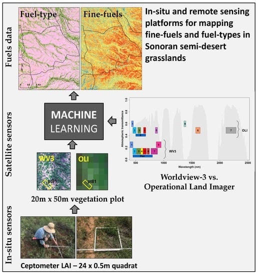
In-Situ and Remote Sensing Platforms for Mapping Fine-Fuels and Fuel-Types in Sonoran Semi-Desert Grasslands


1
US Fish and Wildlife Service, Division of Biological Sciences, Albuquerque, NM 87102, USA
2
Lab of Landscape Ecology and Conservation Biology, Northern Arizona University, Flagstaff, AZ 86011, USA
*
Author to whom correspondence should be addressed.
Remote Sens. 2018, 10(9), 1358; https://doi.org/10.3390/rs10091358
Submission received: 28 July 2018
/
Revised: 21 August 2018
/
Accepted: 21 August 2018
/
Published: 27 August 2018
/
Corrected: 19 June 2023
(This article belongs to the Section Remote Sensing in Agriculture and Vegetation)
Abstract
:Fire has historically played an important role in shaping the structure and composition of Sonoran semi-desert grassland vegetation. Yet, human use and land management activities have significantly altered arid grassland ecosystems over the last century, often producing novel fuel conditions. The variety of continuously updated satellite remote sensing systems provide opportunities for efficiently mapping combustible fine-fuels and fuel-types (e.g., grass, shrub, or tree cover) over large landscapes that are helpful for evaluating fire hazard and risk. For this study, we compared field ceptometer leaf area index (LAI) measurements to conventional means for estimating fine-fuel biomass on 20, 50 m × 20 m plots and 431, 0.5 m × 0.5 m quadrats on the Buenos Aires National Wildlife Refuge (BANWR) in southern Arizona. LAI explained 65% of the variance in fine-fuel biomass using simple linear regression. An additional 19% of variance was explained from Random Forest regression tree models that included herbaceous plant height and cover as predictors. Field biomass and vegetation measurements were used to map fine-fuel and vegetation cover (fuel-type) from plots on BANWR comparing outcomes from multi-date (peak green and dormant period) Worldview-3 (WV3) and Landsat Operational Land Imager (OLI) imagery. Fine-fuel biomass predicted from WV3 imagery combined with terrain information from a digital elevation model explained greater variance using regression tree models (65%) as compared to OLI models (58%). Vegetation indices developed using red-edge bands as well as modeled bare ground and herbaceous cover were important to improve WV3 biomass estimates. Land cover classification for 11 cover categories with high spatial resolution WV3 imagery showed 80% overall accuracy and highlighted areas dominated by non-native grasses with 87% user’s class accuracy. Mixed native and non-native grass and shrublands showed 59% accuracy and less common areas dominated by native grasses on plots showed low class accuracy (23%). Digital data layers from WV3 models showed a significantly positive relationship (r2 = 0.68, F = 119.2, p < 0.001) between non-native grass cover (e.g., Eragrostis lehmanniana) and average fine-fuel biomass within refuge fire management units. Overall, both WV3 and OLI produced similar fine-fuel biomass estimates although WV3 showed better model performance and helped characterized fine-scale changes in fuel-type and continuity across the study area.
1. Introduction
Fuel and fire hazard estimates from remotely sensed data are frequently sought because of the prevalence of wildland fires in the western US and the need to assess potential fire behavior [1]. While a great deal of attention has been paid to characterizing forest canopy fuels [2], fewer efforts have focused on estimating arid grassland fuel conditions [3,4]. For grassland ecosystems, fire rates of spread and intensity are driven by the amount and continuity of fine-fuels, in addition to fuel moisture, fire weather conditions, and topography [5]. Fine-fuel biomass (termed ‘fine-fuel’ from here onward) in semi-desert grasslands principally pertains to the above ground portion of flammable herbaceous plant material per unit of area (e.g., grasses and forbs), that is important to fire spread and intensity. Fine-fuels in arid grasslands are increasingly dominated by non-native plants that can increase fuel loads (herbaceous and woody fuels combined) and continuity, necessitating assessment of hazardous fuels that may threaten animal habitat, water quality, human infrastructure, and other natural resource values [6,7].
Fine-fuels and fuel-type (e.g., grass, grass-shrub, tree, woody debris) are principal vegetation parameters needed to assign fuel model types used as inputs to fire behavior models [8]. Fire behavior models such as FlamMap, FARSITE, and BEHAVE require fuel model types representative of fuel conditions to help determine potential fire behavior such as rates of spread, minimum travel time, and transition from a surface to crown fire [9,10,11,12]. Fuel characteristics are frequently obtained from remote sensing which offers an increasingly diverse set of tools for mapping surface and canopy fuels [4,13,14].
The recent increase in the number and variety of private and public sector satellite remote sensing systems provide an enhanced means of estimating grassland fuel parameters. Programs aimed at increasing commercial remote sensing space activities through the US president’s Commercial Remote Sensing Space Policy (CRSSP; https://crssp.usgs.gov/) dramatically improve access to high spatial and temporal resolution imagery [15]. Improved access and flexibility to acquire high spatial resolution (0.30 m to 5 m pixels) satellite data for a specific area and time interval is particularly important to US land management agencies that must prioritize fire and fuels monitoring and mitigation activities. Satellite systems such as WorldView-1:4, GeoEye, and IKONOS, RapidEye, SkySat-1:2, and PlanetScope provide detailed panchromatic and multispectral imagery at a spatial resolution previously only captured by airborne systems. Worldview-2 and Worldview-3 are also capable of a 1–4-day revisit time making appropriate timing of image capture more feasible. This is particularly beneficial in grassland ecosystems which can exhibit strong spatial and temporal differences in plant productivity in conjunction with precipitation patterns or disturbance [16,17]. WorldView-3 (WV3), a commercial system, captures spectral reflectance data in the coastal (400–452 nm), blue (448–510 nm), green (518–586 nm), yellow (590–630 nm), red (632–692 nm), red-edge (706–746 nm), near-infrared1 (772–890 nm) and near infrared2 (866–954 nm) ranges at a 1.24 m pixel size. Landsat Operational Land Imager (OLI), an open access public system, captures reflectance data in the coastal (430–450 nm), blue (450–510 nm), green (530–590 nm), red (640–670 nm), near infrared (850–880 nm), shortwave infrared (1570–1650 nm), shortwave infrared2 (2110–2290 nm), and cirrus (1360–1380 nm) spectral ranges at a 30 m pixel size (Figure 1). Each sensor provides a 12-bit dynamic range and improved signal-to-noise radiometric performance over previous 8-bit sensors, important for vegetation monitoring and above ground biomass estimation [18,19].
Concurrently, the availability of affordable ground-based sensors has also increased. Vegetation index (VI) values taken from ground-based sensors (e.g., radiometer) such as the normalized difference vegetation index (NDVI) are capable of generating reliable grassland biomass and fuel moisture estimates [20]. Relatively low-cost devices offer rapid and automated measurement of spectral reflectance data and plant parameters such as the photosynthetically active radiation (PAR), NDVI, photochemical reflectance index (PRI), and leaf area index (LAI). Ground-based sensors are useful in combination with satellite and other field observations for developing landscape to region-scale predictions of variables such as above-ground biomass, agricultural yields, CO2 uptake, and water stress [21]. In particular, LAI, defined here as the amount of leaf surface per unit area of ground, is highly correlated with plant biomass [22,23]. PAR is the downwelling solar radiation in the 400 nm to 700 nm spectral region that is the portion of the electromagnetic spectrum used by plants for photosynthesis. Therefore, PAR intercepted by plant canopy is measured using in-situ sensors to estimate canopy structural parameters and calculate LAI [24].
The principal objectives of this study were to examine in-situ and remote sensing techniques important for accurately mapping semi-desert grassland fuels from a new generation of remote sensing systems. To accomplish this, we sought to compare non-destructive LAI estimates with more conventional field measurements. Therefore, quadrat-scale measures of clipped above ground herbaceous biomass were compared with field-ceptometer (Decagon Devices Accupar LP-80; http://www.decagon.com/) PAR measurements used to calculate LAI and model fine-fuels. Plot- and quadrat-based vegetation measurements were also used to map fine-fuels from both WV3 and OLI satellite data. From previous studies, we anticipated that that VI developed from the WV3 red-edge spectral region (706–746 nm) would improve biomass estimates over other VI typically developed from OLI or earlier Landsat satellite imagery [18,19]. In addition, we mapped land cover (i.e., fuel-types) identified from field plots and WV3 imagery to assess VI, spectral bands and cover estimates (e.g., herbaceous plant cover vs. percent bare ground) helpful for improving classification accuracy and developing fuel inputs needed for defining grassland fuel-types and fire behavior modeling [25].
Vegetation indices combine spectral bands to enhance sensitivity to changes in vegetation leaf area index, greenness, and biomass [26]. Vegetation indices utilizing the red-edge spectral region that is sensitive to shifts in canopy biomass and chlorophyll content have proven important for biomass estimation in previous studies [18,19,27]. Likewise, shortwave infrared bands have helped to reduce soil background effects that can interfere with biomass estimates from remotely sensed data [28,29] and enhance estimates of senescent vegetation [30]. For this study, we examined VI and other spatial data that could potentially improve biomass estimation noted from previous studies [18,19,31].
We focused our study on semi-desert grasslands in the southwestern US. Semi-desert grasslands represent a significant portion of arid landscapes in southern Arizona, New Mexico, Texas, and northern Mexico. More than 5 million hectares likely exist between the US and Mexico that continue to play an important role in the region’s economy and ecological diversity [32]. Frequent low-intensity fires at 8–10 years intervals were once common and maintained semi-desert grassland vegetation composition and structure across the Southwest [33]. Fire can also temporarily enhance soil nutrient environments by volatilizing nitrogen and organic carbon while reducing competition between woody plants and herbaceous vegetation [34].
Nevertheless, arid grasslands have undergone widespread vegetation changes since Euro-American settlement beginning in the late 1800s [35]. While it is challenging to estimate historical conditions, repeat photography, land survey records, and written descriptions suggest that today’s arrangement and diversity of grasses, woody plants or mixed composition vegetation often differ strongly from historical grasslands [32,36]. For many areas, land use practices over the last century such as intensive livestock grazing during alternate periods of drought and wetter phases have subsequently lead to fire-regime disruption and increase cover by woody species such as Prosopis spp. (Mesquite) [34,37]. Others have found that a cessation of indigenous utilization of mesquite has also contributed to its expansion over the last century or more [36,38]. Increased woody plant cover can thus alter site thermal and moisture environments, herbaceous plant production, and disturbance regimes [17]. In some cases, these impacts have ultimately led to a long-term conversion of mixed grass and shrublands to woodland vegetation [39].
The introduction of non-native invasive grasses is also recognized as a primary change agent affecting semi-desert grassland fuel production. On suitable sites, an increased abundance of highly competitive non-native grasses has led to reduced plant diversity and increased fine-fuel loads that can alter fire behavior [40,41]. Non-native and drought tolerant African grasses such as Eragrostis lehmanniana (Lehmann lovegrass) and Cenchus ciliari (buffelgrass) were initially planted for erosion control and improved animal forage starting in the 1930s [40,42]. Each of these perennial bunch grasses has since spread to unplanted areas often following disturbances and drought periods transforming the amount, composition, and distribution of fine-fuels in semi-desert grasslands [6,43].
We ultimately sought to improve methods for developing digital data layers depicting fine-fuels and fuel-types that can be used to model potential fire behavior and inform land planning decisions with respect to vegetation and fire management. Therefore, primary objectives were to (1) develop effective and rapid non-destructive field sampling methods that can accurately determine fine-fuel biomass within semi-desert grassland conditions; (2) assess a set of satellite derived spectral predictors, VI and spatial variables (e.g., terrain and vegetation cover estimates) for mapping fine-fuels; (3) compare fine-fuel biomass models from WV3 imagery to more conventionally used OLI predictor variables; and (4) develop and assess image classification of existing vegetation needed for assigning fuel model types. Comparisons were also made to assess fuel conditions within the study area using digital fuels data.
2. Materials and Methods
2.1. Study Area
The study area encompasses the 48,000 ha Buenos Aires National Wildlife Refuge (BANWR) that was established in 1985. BANWR is located in the Altar Valley of southern Arizona boarding with Mexico that is situated between several small mountain ranges running north and south to the Mexican border (Figure 2). The refuge was principally established to facilitate recovery of the critically endangered masked bobwhite quail (Colinus virginianus ridgwayi) within the US and northern portion of its range [44]. BANWR itself is divided into 85 separate management units, primarily for prescribed burning purposes, as well as distinct management zones, developed for focusing masked bobwhite habitat restoration activities in suitable areas. The 9300 ha masked bobwhite management zone covers priority areas at lower elevation areas and drainage networks in the Altar Valley. An extended masked bobwhite zone encompasses an additional 8600 ha occupying slightly more upland sites which likely contained suitable habitat conditions historically.
Climate is semiarid with low precipitation and humidity and high summer temperatures. Temperatures range from −11 °C in winter to 41 °C in summer. Summer and winter temperatures average 33 °C (May–September.) and 18 °C (December–February) respectively. Precipitation averages 43 cm annually and is bimodal with approximately 40% occurring during July and August and the remaining during winter according to the Sasabe, AZ weather station (http://www.wrcc.dri.edu/) that is located at the extreme southern end of BANWR. Anvil Ranch weather station, 19 km to the north, shows a much lower annual precipitation (29 cm) indicating an increasing north to south precipitation gradient. The valley floor is intersected by numerous dry washes that create level to hilly terrain ranging in elevation from 925 m to 1400 m. Soils are well drained and coarse to moderately fine textured Aridisols and Mollisols [45].
Prior land use was principally intensive livestock grazing by cattle since the 1880s. Extensive removal of Prosopis velutina (Velvet mesquite) during the 1970s and early 1980s was used to improve forage production [46]. Some rangeland seeding treatments were also applied during this period, in the northern portion of the refuge with a mix of Panicum antidotale, Sorghum halepense, Leptochloa dubia, and E. lehmanniana primarily in drainage bottoms (unpublished data). Upland areas in the northern portion of BANWR were also apparently seeded with a mix of Eragrostis chloromelas, Eragrostis intermedia, E. lemanniana, and L. dubia that covered approximately 7500 ha. Historical patterns of land use and hydrologic changes have resulted in a mixture of native and non-native vegetation on the BANWR [47]. E. lehmanniana currently dominates most upland sites, in addition to other non-native grasses including Eragrostis chlormelas and Eragrostis superb. Common native grasses include Boutaloua spp., Sporobolus spp., Aristida spp., Bothriochloa barbinodis, and Digitaria californica. Deep soils in drainages and disturbed bottomlands include Sorghum halepense, Sporobulus spp., Amaranthus palmeri, and Salsola kali. P. velutina is the dominant tree on BANWR, but other species such as Celtis spp. and Acacia spp. are also common. Other common woody shrubs and subshrubs include Isocoma tenuisecta, Gutierrezia sarothrae, Caliandra eriphylla, Acacia spp., Mimosa spp., and Atriplex canecense. The largest plant family is Asteraceae, with a marked diversity of annual and perennial forbs and subshrubs. Upper elevations between 1200 m and 1800 m areas contain areas of dense shrublands such as Mimosa Dysocarpa and perennial graminoids giving way to Madrean evergreen woodlands dominated by Quercus oblongifolia, Juniperous deppeana, and Pinus engelmannii.
Since refuge establishment, prescribed fire has been used as a primary management tool, in addition to some mechanical treatments to remove P. velutina for improving habitat conditions for the masked bobwhite and, more recently pronghorn (Antilocarpa americana). A majority of management units at low elevations in the central portion of the refuge have been burned at least once with several of them being purposefully burned or burned by wildfires between three and five times in the last 30 years.
2.2. Vegetation Measurements
2.2.1. Plant Cover
Vegetation cover data were collected from 20 m × 50 m rectangular plots on BANWR using stratified random sampling design during two separate periods. Vegetation plots measured across the refuge between July and October of 2012 and 2013 (n = 207) were within vegetation strata defined by dominant life form classes (i.e., trees, shrubs, and herbaceous plants), and three elevation categories roughly classed as valley bottom, foothills, and Madrean physiographic environments (Figure 2). On each plot, we measured 6, 20-m point intercept transects spaced 10 m apart recording plant species and soil substrate at 0.5 m intervals. Species intercepted were recorded in three height classes there between 0.0.and 0.5 m, 0.5 and 2.0 m, and >2.0 m. Plot locations were also stratified by low, medium and high productivity categories based on NDVI from a 2011 Landsat Thematic Mapper (TM) image taken during the peak growing season.
Vegetation plots measured between July and October of 2014 and 2015 (n = 239) used the same measurement techniques above, but with the addition of fine-fuel quadrats, that were part of a separate study examining contemporary fire-effects on semi-desert grassland vegetation and masked bobwhite habitat. As such, we confined plots to the masked bobwhite management zone and extended management zone in the valley bottom. These plots were stratified based on fire history and local hill-slope position which can influence soil physical properties and site moisture regime as well as disturbance characteristics such as fire behavior. Specifically, we used the US Fish and Wildlife Service Fire Atlas and a record of fire perimeters (polygons) measured between 1985 and 2015 to estimate fire frequency on BANWR. Perimeter data were converted to a raster in a geographic information system (GIS) representing the location of fires for each year which was used to calculate the number of fires occurring within a 30 m grid cell over a 30-year period. Fire frequency was divided into low (0–2 fires), medium (3–4 fires) and high (≥5 fires) strata. We used the 10 m digital elevation model (DEM) from the USGS National Elevation Dataset to calculate topographic wetness index (TWI) values using Taudem v. 5.0 software (http://hydrology.usu.edu/taudem/taudem5/index.html) executable files in the R statistics package v. 3.1.1 [48]. Three terrain classes were visually defined as drainage, ridges and steep slopes, and footslope classes using a detailed DEM and hillshade map developed from 2007 airborne laser altimetry (LiDAR) tiles that were limited to borderland areas obtained from the USGS Earth Explorer website (https://earthexplorer.usgs.gov/). The R statistics ‘sampling’ package v. 2.8 [49] was used to create an equal number stratified random plots within fire frequency and terrain classes.
All plot corners were georeferenced in the field with a Trimble GeoXT or Geo7X and post-processed to differentially correct point locations to within 1m positional accuracy using Trimble Pathfinder Office v.5.60 [50].
2.2.2. Grassland Fine-Fuels
We used a double sampling approach to measure fine-fuels to develop non-destructive measurements for more efficient sampling during the 2014 and 2015 field study. Therefore, grassland fuels were first sampled on n = 20, 20 m × 50 m plots within 24, 0.5 m × 0.5 m quadrats spaced 5 m apart along 6, 20-m transects. Destructively sampled quadrats were measured during August of 2013, the month typically at or near the peak of the growing season. All herbaceous plants within quadrats were clipped to the ground and taken to a lab to be oven dried at between 60 °C and 70 °C for at least 48h and weighed to the nearest 10th of a gram. We also recorded the height and percent cover of grasses, forbs, cacti, and woody plants in each quadrat. Herbaceous plant cover was visually estimated on quadrats and average canopy height was measured with a metal tape to the nearest centimeter.
Prior to plant measurements and clipping, we used an AccuPAR LP-80 ceptometer to record leaf area index (LAI) at five locations spaced 10 cm apart inside the quadrat. An external sensor and the ceptometer were used together to simultaneously measure above and below canopy PAR (400–700 nm), at a resolution of 1 µmol m−2 s−1 within a range of 0 to 2500 µmol m−2 s−1. Above and below canopy PAR measurements in addition to sun zenith angle (z), fraction of beam radiation (Fb), and a leaf distribution parameter (X) set to 1 for desert grasses were used to instantaneously calculate LAI. The mean LAI value per quadrat was then calculated from the five samples and stored on the ceptometer control box. Occasionally, shaded quadrat locations or those showing >10% woody plant cover were relocated to the next 1 m interval along the transect to avoid shading impacts on herbaceous LAI measurements. Quadrat measures were generally taken on the east side of transects prior to noon and the west side of transects in the afternoon to avoid observer shadows over quadrats.
We then used 2013 destructive samples to parameterized herbaceous biomass models, detailed below, that were used to non-destructively estimate herbaceous biomass on plots measured during years 2014 and 2015 (n = 239). Pending sufficient biomass model performance, all future quadrat samples used only ceptometer LAI, herbaceous plant canopy height, and visual cover measurements to estimate fine-fuels with the same procedures detailed above.
2.2.3. Remotely Sensed Data
For developing digital data needed to estimate fine-fuel biomass and fuel-type on BANWR, we acquired cloud-free Digital Globe WV3 imagery from September (peak green period) and November (senescence period) of 2015 using the CRSSP Imagery-Derived Requirements (CIDR) Tool (https://crssp.usgs.gov/). Cloud-free and terrain corrected OLI imagery with a 30 m pixels size was also acquired from the USGS EarthExplorer website (https://earthexplorer.usgs.gov/) for June (senescence period) and August (peak green period) of 2015 (Path 36/Row 38). WV3 image data were orthorectified and resampled to a 10 m pixel size for analyses using ERDAS Imagine v. 15.0 [51]. We converted all image data to surface reflectance with the ENVI v. 5.3 Fast Line-of-Site Atmospheric Analysis of Hypercubes (FLAASH) module [52].
In addition to WV3 and OLI spectral bands, reflectance data were used to create multiple VI such as NDVI, soil adjusted vegetation index (SAVI), and enhanced vegetation index (EVI) designed to improve biomass estimates and land cover classification [26,53]. As bands from each senor-type cover different spectral ranges, we created a set of VI specific to each sensor. For WV3, we contrasted 27 VI using band combinations in red, red-edge (RE), and near infrared (NIR) spectral regions (Table 1). Alternatively, we developed a set of 12 VI using red, NIR, and shortwave infrared bands (SWIR) from OLI surface reflectance data. VI from each sensor differed in that WV3 had no SWIR band combinations and OLI had no RE band combinations (Table 1). Therefore, indices such as the Soil Adjusted Total Vegetation Index (SATVI), Total Vegetation Fractional Index (TVFC), and a standardized greenness-to-cover index (GCI) that use SWIR bands were only calculated from OLI images [30,54]. We also used the difference between peak green period and senescence period image dates and VI to better distinguish fine-fuels in mixed vegetation comprised of grass, shrubs, and trees. A principal components rotation of the spectral bands for each sensor type was also used as predictor variables and possible means to reduce data dimensionality.
2.2.4. Data Analysis
In-Situ Biomass
We used destructively sampled biomass from all effectively sampled quadrats (n = 431) on 20 plots measured in August of 2013 to develop and test predictive biomass models. We evaluated which variables measured on quadrates were most important to accurately predict herbaceous biomass and which non-destructive measures could accurately estimate fine-fuel loads. Therefore, Random Forest regression tree models [63] were used to predict dry weight (g/m2) herbaceous biomass (i.e., grasses and forbs) from explanatory variables that were LAI, percent cover, and average height for each plant life-form. Random Forest (RF) classification and regression trees, often used with high-dimensional data, provided a flexible approach to both estimate fuel parameters on plots and map fuel-types from remotely sensed data that is described below.
Random Forest is a ‘tree-based’ machine learning method that uses multiple bootstrap samples of the data with replacement to train classification and regression models [63]. Samples held out of training, typically one-third, are then used to evaluate model performance using the root mean squared error (RMSE) and the proportion of variance explained for regression. Overall and percent class error is used to evaluate classification model accuracy. Performance measures calculated for model iterations are aggregated at the end of training to assess error. Predictors are also randomly selected and tried at each node in a tree and iteratively withheld from trees to estimate their level of importance. Therefore, each variable’s importance is evaluated by assessing model performance with and without its presence in the model for as many model iterations as requested. Random variable selection along with bootstrapped error aggregation, known as ‘bagging’, have proven to be an effective means for identifying the most important variables in the model and assessing model error [64]. Therefore, an increase in percent mean squared error (MSE) or ‘node purity’ with a variable left out of a model training at each iteration is a measure of its overall importance.
For this study, we used the ‘caret’ package v. 6.0-76 [65] for classification and regression model training and recursive feature elimination (RFE) available for R statistical software to develop RF biomass models. RFE is a backwards variable selection process that progressively eliminates the least important predictors [66]. For developing final models, an optimized number of predictors were selected based on the lowest RMSE obtained from 10-fold cross validation. A model tuning algorithm was also applied to optimize the RF parameter ‘mtry’ which is the number of predictors randomly selected for each node. An iterative approach was taken by adding a successively greater number of predictors to each RF node split. The mtry parameter was set in the final RF model by selecting the number of available predictors at a node that showed the greatest decrease in model error rate. A final best performing set of predictors and model was ultimately selected for estimating biomass from non-destructively sampled quadrats on future plots with LAI measurements. Ordinary least squares (OLS) regression was also used to investigate single variable biomass predictions that could help to reduce field measurement time.
Remotely Sensed Fine-Fuel Biomass
We used herbaceous biomass measurements only available from 2014 and 2015 plots (n = 239) to model and map fine-fuel loads with WV3 and OLI imagery. To compare sensor types, we developed similar sets of spectral bands and VI as predictors as well as those using differing spectral regions captured by each sensor type (Table 1). To improve predictions we also developed a set of principal cover data layers likely to help estimate fine-fuel biomass such as the percent cover of bare ground, woody vegetation (shrubs and trees together), as well as trees and herbaceous plants from all plots measured between 2012 and 2015 (n = 446). No disturbances had taken place on plots up to the time that satellite image data was collected and all plots were measured during the principal growing season. As with quadrat-scale methods described above, we used RF regression tree and RFE model training techniques to predict fine-fuel biomass from each sensor type and evaluate model performance. Therefore, the mean value of predictor variables and pixels within plot boundaries were used to develop model training data using zonal statistics in the ‘raster’ r-package v. 2.5-8 [67]. Plot rectangles were buffered by 5 m to accommodate OLI 30 m pixels and generate mean plot values for each predictor. For making cross-sensor comparisons, we used mean spectral values from plots to reduce potential scale effects from the two sensor types at a 10 m and 30 m pixel size. We used variable importance metrics to compare each set of predictors anticipating that red-edge bands and difference VI from leaf-on and leaf-off imagery would improve model accuracy (Table 1). Scatter plots and modified t-tests [68], that account for spatial correlation among plots, were then used to make statistical comparisons between WV3 and OLI biomass estimates at plot locations.
Remotely Sensed Vegetation Cover
To map vegetation cover that is the basis for assigning fuel model types [8], we used plant species data and cover estimates from all 446 plots and WV3 imagery only. Plot data were used to assign classes following the US National Vegetation Classification System hierarchy (NVC, http://usnvc.org/). To aid classification, we used Bray–Curtis similarity and the Flexible-beta cluster analysis in the ‘cluster’ v. 2.0.6 r-package [69] to group plots by plant species composition and develop a training data set for vegetation classification models. We used K-means partitioning with canopy cover data for all species with >1 occurrence to determine an optimal number of vegetation classes. This resulted in six principal vegetation classes from plot data (Table 2). Five additional categories for rare or un-sampled land cover types such as urban development, water bodies, bare ground, and closed canopy tree cover were identified from 2013 National Agricultural Imagery Program (NAIP) digital aerial photographs and 2015 WV3 0.5 m panchromatic imagery. Sample locations were visually selected from NAIP and WV3 imagery to develop land cover classification inputs in addition to plot data.
We used plots classified by vegetation type and high-resolution imagery for each land cover class for developing RF classification models. A tuning algorithm was used to define the optimal number of predictor variables tried at each node and RFE was used to select an optimal subset of predictors. We used samples left out of training at each model iteration to estimate ‘out of bag’ (OOB) error that was averaged over the number of trees requested during model training (n = 2000). Model performance was assessed using overall classification error and user’s and producer’ accuracy for individual land cover categories [70]. We assessed variable importance from RF models for principal vegetation categories to compare and contrast WV3 spectral bands and indices useful for discriminating specific classes.
3. Results
3.1. In-Situ Biomass Results
Herbaceous biomass clipped from n = 431 quadrats on 20 plots ranged from 0.0 g/m2 to 741.6 g/m2 and averaged 103.1 g/m2 ± 102.0. Using 10-fold cross validation as our RFE training control methods for feature selection, six of the 10 variables used for predicting fine-fuel biomass were selected as optimal using minimum RMSE values (Figure 3). We used the selected optimal predictors to further tune the number of variables tried at each node for RF models. Two predictors tried were found to more substantially decrease OOB error and were used in the final RF model with six selected predictors. The final model resulted in 84% of the variation explained and a root mean squared error (RMSE) of 3.88 g/m2. From variable importance plots, we found that ceptometer LAI was the most important predictor variable when compared to all other quadrat-scale predictors. Both percent MSE and node purity increased similarly with LAI held out of RF models (Figure 4A.B). Other variables such as total plant cover were highly correlated with LAI (r = 0.87), and subsequently removed from the final model through backwards elimination. While not a focus for this investigation, multiple linear regression performed similar to RF using all six square root transformed predictors (r2 = 0.84, F = 462.3, p < 0.001).
We also assessed simple linear regression models with selected LAI, cover and height variables as predictors which explained 18% to 40% less variance than RF models, but showed a strong positive relationship with dry biomass (Figure 5A–D). The final RF model from destructive samples was then used to predict non-destructively sampled quadrats on all plots measured in 2014 and 2015 which showed similar average cover (%) and height (cm) estimates to those collected on quadrates in 2013 respectively ( = 27.6 ± 24.1 vs. = 31.9 ± 27.3, = 11.7 ± 6.8 vs. = 8.5 ± 5.4). Predicted biomass for non-destructively sampled plots ranged from 104.3 kg/ha to 3339.6 kg/ha and averaged 1363.0 ± 649.2 kg/ha, which was within the range of values previously reported by Marsett et al. [30] for Sonoran and Chihuahuan rangelands with a burning and grazing history.
3.2. Remotely Sensed Fine-Fuel Biomass Results
We first derived continuous cover data from vegetation plots and satellite imagery for general classes of vegetation (herbaceous, woody plants, and trees) and bare ground to add as predictor variables to spatial models of fine-fuel biomass. These models resulted in four separate data layers from each sensor type. Random Forest and RFE feature selection models results can be found in Table 3. Both models for WV3 and OLI performed similarly in terms of variance explained and RMSE. Feature selection substantially reduced the number of predictors while increasing variance was explained, particularly for WV3 herbaceous and bare ground models (Table 3). Important predictor variables from cover models are further discussed below in conjunction with biomass models for each sensor type. However, the amount of herbaceous and bare ground cover on a plot was considered important to estimate fine-fuel biomass. For example, a curvilinear model to predict fine-fuel biomass from the ratio of herbaceous to bare ground cover on plots explained a significant amount of variation (r2 = 0.64, p < 0.001, Figure 6). A curvilinear model fit likely resulted from the difference between dense tall grasses versus short-statured forb dominated areas that differ in the amount of herbaceous biomass accumulated on site.
Therefore, three separate fine-fuel biomass models were developed for each sensor type, first using spectral predictors, second with spectral and terrain predictors, and lastly a combined model that included vegetation cover variables. The combined model performed substantially better than either of the two previous sets of predictors for both sensor types (Table 4). The optimal number of predictor variables selected with RFE decreased substantially from 37 to 19 for the WV3 model while the amount of variance explained increased from 51.1% to 65.0% (RMSE = 403.8 kg/ha). Similarly, the number of OLI model predictors was decreased from 43 to 10 while increasing the variance explained from 47.1% to 57.6% (RMSE = 440 kg/ha, Table 4). Further discussion of results considers only comparisons and model outcomes from the two sensors using all variables combined.
In each case RFE reduced the number of predictor variables used, particularly for OLI which decreased from a total of 70 possible to 10 while >20 predictors noticeably increased cross-validation RMSE for both sensor types (Figure 7A,B). Overall, WV3 biomass models performed better than OLI models with 7.4% greater variance explained and 8.3% lower RMSE. Nevertheless, a modified t-test comparing WV3 and OLI biomass predictions, which reduces the effect of spatial autocorrelation, revealed significantly positive correlation (r = 0.85) between model predictions (F = 32.4, DF = 12.0, p < 0.001). A scatter plot comparing predicted versus observed values from plots was also similar between the two sensors with an r2 = 0.70 (p < 0.001) and r2 = 0.74 (p < 0.001) for WV3 and OLI respectively (Figure 8A). In only a small number of cases, WV3 biomass predictions were biased higher relative to plot values, while OLI predictions were biased lower. A direct comparison of fine-fuel biomass predictions by each sensor type indicated a strong positive relationship (r2 = 0.73, p < 0.001) between the two estimates with relatively few plots showing large differences (Figure 8B).
We anticipated that red-edge and SWIR band combinations would be highly important to biomass predictions. Variable importance plots from each sensor type showed that the amounts of bare ground and herbaceous cover taken from digital data layers were overwhelmingly the most important variables for biomass predictions (Figure 9A–D). Improved herbaceous and bare ground cover model performance was largely driven by Yellow, Red, Red-edge and NIR bands and vegetation indices depending on available bands from each respective sensor (Figure 10A–D and Figure 11A–D). EVI and SAVI that contain a soil adjustment factor were among the top 10 variables for herbaceous cover models for both WV3 and OLI, and OLI bare ground models. For WV3 biomass models the Red, Yellow, and Red-edge bands were also among the top 10 important predictors as well as vegetation indices developed from NIR and Red-edge bands from leaf-on and leaf-off imagery. For OLI models, Green, NIR and Coastal bands were among the top 10 important predictors as well as leaf-on indices such as total vegetation fractional cover (TVFC) and the soil adjusted total vegetation index (SATVI) that are sensitive to green and senesced vegetation in semi-desert environments (Figure 9C,D) [30]. Standardized GCI1 and GCI2 (greenness to cover indices) from leaf-off imagery were also important to OLI biomass models as they incorporate NDVI, TVFC, and SATVI that likely help increase sensitivity to lower levels of plant greenness [54]. Other important predictors such as elevation, solar radiation, and the differenced PCA1 band were helpful in reducing data dimensionality for both WV3 and OLI biomass models.
We also found that similar variable combinations improved cover model performance (Figure 11A–D) that, in turn, contributed to comparable and improved biomass predictions from WV3 and OLI models. Random Forest models for herbaceous and bare ground cover also produced highly comparable results and predictions consistent with field plot measurements (Figure 12A,B). Performance measures such as variance explained and RMSE were generally low for WV3 and OLI models (Table 3), but were consistent with plot measurements used as model inputs (Figure 12A,B). OLI had a somewhat stronger relationship to field data collected for herbaceous vegetation (r2 = 0.75, p < 0.001) and bare ground (r2 = 0.72, p < 0.001) than WV3 model predictions (herbaceous r2 = 0.65, p < 0.001; bare ground r2 = 0.66, p < 0.001).
3.3. Remotely Sensed Land Cover
For land cover classification, we focused on WV3 imagery only to develop classes and fuel-types compatible with fine-fuel biomass estimated at a 10 m pixel resolution. A model using all predictors resulted in an overall classification accuracy of 82.7% from validation samples left out of model training. Models using all sample data to assess OOB error achieved 78.0% accuracy. A total of 67 predictors were selected out of 101 using RFE to optimize the classifier. Optimized models resulted in 83.1% accuracy from separate validation samples and 79.6% from OOB error assessment estimated using n = 2000 classification trees (Table 5A,B). Most low elevation sites were dominated or co-dominated by the non-native perennial grass Lehmann lovegrass with sparse native grasses such that very few native plant dominated samples were available for separate model training and validation data sets. Therefore, 25% of samples randomly selected for independent validation, without replacement, were not sufficiently representative for determining accuracy of native grass dominated areas (n = 9) or upland shrub vegetation (n = 4). Because vegetation data were collected from randomly assigned plots spaced at a minimum distance of 250 m apart, we believed that OOB error estimates better reflected class accuracy than separate validation data.
Not surprisingly, predictors with the greatest overall importance for improving class accuracy were related to elevation, topographic roughness, and wetness indices for distinguishing land cover types (Figure 13A,B). Many of the cover types occupied dissimilar terrain conditions within the study area. For example forb and herb dominated sites were typically found within topographic depressions or flat valley-bottom terrain whereas mixed shrub and herbaceous vegetation were within drainage areas with greater mesquite cover. Upland shrubs and Madrean oak–juniper forest were primarily on steep mountain slopes surrounding the Altar Valley. Decreases in Gini were most strongly influenced by predictors combining green and NIR bands that are sensitive to vegetation differences in chlorophyll content and leaf pigment (Figure 13B) [71,72]. Indices such as leaf-on NDWI that are sensitive to areas of increased or decreased moisture were also important, likely helping to distinguish between upland and low-lying vegetation classes (e.g., within drainage bottoms).
Variable importance for individual classes and predictors was highly varied, however vegetation indices incorporating NIR, red-edge, and green bands were most important to distinguishing areas dominated by exotic grasses from other vegetation (Figure 14A). Red-edge and NIR band combinations from the leaf-off image were likely important as non-native Lehnman lovegrass that often retains some photosynthetic material during senescent periods for other native grasses [73]. We found that Lehman lovegrass can comprise as much as 100% cover on our intensively sampled plots (n = 240 intercepts per 0.10 ha−1 plot), while native grasses were often sparsely distributed. Native grasses were best distinguished using a combination of yellow and red bands, although class accuracy was low because of confusion with exotic grasses and mixed grass and shrubland categories (Figure 14B, ≤23.1% user’s accuracy). We sampled very few plots dominated by native grasses, which were often a minor portion of the plant composition relative to Lehman lovegrass cover. Therefore, far fewer samples were allocated to a native grass category for model training which required a greater proportion of native to non-native grass cover on plots.
Oak–juniper woodlands are primarily evergreen which were largely distinguished from upland and other shrub vegetation with leaf-off spectral bands (Figure 14D–F). All other land cover categories were classified with accuracies ≥84.2% primarily with leaf-on spectral bands and indices as most important to class accuracy (Figure 14G–K). An exception was tree cover that was lower elevation dense canopy trees within principal drainages, where a combination of leaf-on and leaf-off bands as well as topographic variables that were important to accuracy (Figure 14G).
4. Discussion
As greater monetary and human resources become essential to mitigating hazardous fuels and fire impacts on natural resource and other values; a means to assess fuel conditions and potential fire behavior is increasingly important [74]. Frequent-fire is historically characteristic of semi-desert and other arid grasslands in the western US; yet average fire season length and fire size have increased over the last three decades [75,76]. Historical and contemporary land use; climate-change and fire management practices can also, in places, increase fine-fuel loads particularly where non-native grass invasions have become extensive [77,78,79,80,81].
Our findings indicated that recent advances in satellite and in-situ sensors show promise for improving estimates of fine-fuel conditions at spatial and temporal scales important to land managers [18,21,27,82]. Overall, non-destructive field measurements and satellite data were effective for estimating fine-fuel biomass in semi-desert grasslands. We found that in this landscape, field ceptometer measurements combined with WV3 or OLI image data produced biomass estimates well within the range of anticipated values for semi-desert grasslands. Biomass values measured on our plots were closely aligned with the field estimates previously obtained by Marsett et al. [30] from other semi-desert grassland sites in southern Arizona.
Field ceptometer LAI combined with average herbaceous plant height and cover provided rapid and accurate field biomass predictions where minimal woody plants (μ < 2%) and cacti (μ < 1%) were encountered within 0.5 m2 quadrats. Measurements of plant height and canopy cover by life-form added time to quadrat sampling, but helped explain an additional 10% of the variation in fine-fuel biomass with RF models. Sharma et al. [20] also found that canopy height measurements improved grassland biomass predictions on 0.25 m2 quadrats when combined with field spectrometer bands and NDVI measurements. While other studies have suggested that LAI can, at times, be cumbersome to measure in grasslands when instrumentation is affected by sky conditions or obstructions near the ground [30], we found that the ceptometer was simple to calibrate and could be efficiently applied within quadrats. As most sample sites in our study areas were dominated by herbaceous cover, systematically selecting quadrat locations and occasionally relocating them to avoid ceptometer shading was feasible in this study area. Sites with greater woody plant cover or succulents such as woodlands or Sonoran Desert uplands would likely require other methods to estimate fine-fuel biomass from field measurements. Overall, LAI was the best predictor of fine-fuel biomass and total herbaceous plant cover was the second best predictor. In the absence of ceptometer equipment to measure LAI, quadrat measurements of herbaceous plant cover and height may also work well in place of destructive methods.
Remotely sensed biomass models from both WV3 and OLI imagery showed similar, but sufficiently different levels of performance, 65% and 57.6% of variance explained, respectively. OLI model performance also differed from results reported by Marsett et al. [30], who used single date Landsat Thematic Mapper (TM) image VI for Sonoran semi-desert grasslands producing biomass models that explained 77% of the variance. Differences are possibly a result of the larger 90 m × 150 m plots sizes that were more appropriate to 30 m Landsat pixels, but also could be attributed to a low number of validation samples obtained (n = 9) to assess model predictions [30]. Our 20 m × 50 m plot size was designed to fit within specific hillslope categories for assessing soil and other site differences important for measuring masked bobwhite habitat conditions [83]. Thus, plot dimensions differed somewhat from the OLI pixel size (30 m × 30 m) and may have impacted biomass model results, yet final model estimates were highly correlated with WV3 model results (Figure 8A,B). We also avoided occasional shrubs on quadrats and focused principally on measuring herbaceous plants that were the primary fraction of fuels important to fire hazard, behavior, and rates of spread [77]. This may have decreased model performance in areas that occasionally had a greater abundance of woody sub-shrubs such as Gutierrezia sarothrae that were not included in fine-fuel measurements.
Random forest models used with this study allowed for robust model validation by iteratively sampling all plot data (n = 239) over 2000 separate regression tree models to generate bootstrapped error predictions. We considered our assessment an accurate representation of model performance because plots were randomly assigned to sites with differing fire histories and hillslope conditions that were spaced ≥250 m apart (Figure 2). Roadside conditions that can affect vegetation productivity and interfere with sampling (e.g., plots overlapping roadways) were also avoided. WV3 model performance in our study area was similar to results obtained by Muntanga et al. [18] who used single image Worldview-2 (WV2) VI for biomass estimates in a grass dominated wetlands of South Africa. They attained nearly identical r2 (0.79 vs. 0.76) and RMSE (0.438 kg/m2 vs. 0.442 kg/m2) values from best performing RF models evaluated from calibration and independent validation data held out of model training. Greater vegetation cover heterogeneity in our study area between grasses, annual forbs, woody plants, and bare ground may also explain why we found somewhat lower biomass model performance with similar WV3 imagery. Ramoelo et al. [19] achieved greater model performance (r2 ≥ 0.84, RMSE ≤ 105.6 g/m2) from seasonal WV2 imagery and more homogeneous grassland plots in the Kruger National Park, South Africa.
Our biomass model outcomes differed more strongly with results obtained by Sankey et al. [84] who found little or no relationship between single date WV2 image VI and herbaceous biomass measurements on other Sonoran Desert sites. Hot desert locations sampled in their study area were only occasionally dominated by native and non-native annual grasses and forbs (e.g., Schismus spp. and Brassica tournefortii) that can form more continuous fuel-bed conditions only during wetter years [85]. Field measurements showed an average of <1 g/m2 and <10% cover on plots suggesting that trace amounts of herbaceous plant biomass are insufficiently estimated at the spatial and spectral resolution of WV2 or, by extension, WV3 imagery [84]. In contrast, our plots averaged 136.3 g/m2 biomass and 67% cover by herbaceous plants.
RFE methods used to optimize regression tree models substantially improved model outcomes while decreasing the number of predictor variables, consistent with Mutanga et al. [18]. In our study area, estimates of percent bare ground and herbaceous cover were the most important predictors for both WV3 and OLI models (Table 4). Bare ground predictions for WV3 models were considerably improved by yellow, red, and red-edge bands, band combinations and contrasting leaf-on and leaf-off imagery (Figure 11A,B), as SWIR bands for developing conventional soil indices were not available. Nevertheless, OLI bare ground models incorporating bands and indices such as the Normalized Difference Soil Index (NDSI) known to improve discrimination between soil, vegetation, and water [86] showed lower variance explained (Table 3).
More recent studies by Mutanga et al. [18] and Ramoelo et al. [19] found that narrow band WV2 VI using visible and red edge bands were most important for predicting biomass in more densely vegetated South African grasslands. Indeed, we found WV3 red-edge VI were among the most important variables for predicting herbaceous cover that was important to our biomass models. However, the difference in PCA bands 1 and 2 from leaf-on and leaf-off VW3 imagery, that contained 98% of the cumulative variance among spectral bands, was most important to herbaceous cover predictions. PCA bands contributed to the lower number of variables selected (n = 27) in contrast to OLI models that used a greater number of variables (n = 40) and showed lower performance (Table 3). PCA bands selected from RFE likely helped to reduce the overall number of predictors as well as the correlation among predictors. In addition, topographic variables were important in predicting both herbaceous cover and bare ground that have been shown to help explain differences in herbaceous biomass for grasslands elsewhere [87]. Differences in soil texture, solar radiation, and moisture that are related to topography are known to drive vegetation productivity, fine-fuel conditions, and fire occurrence in semi-desert environments [88].
Lastly, we found that land cover data developed from plots and multidate WV3 imagery showed promise for identifying important fuel-types within the study area that have a different potential for carrying a fire. In particular, Lehmann lovegrass can produce up to four times greater annual biomass than native grasses adding significant fine-fuel in areas where it is abundant [40]. We found that locations with high biomass mapped within the study area showed considerable overlap with exotic grasses (Figure 15A,B). A direct comparison between principal fire management units in the Altar Valley (n = 59) showed a significant and strong positive relationship between average unit biomass and non-native grass cover (Figure 16, r2 = 0.68, F = 119.2, p < 0.001). Factors such as fire frequency, precipitation, and soil differences across BANWR likely explain increased non-native grass cover within some management units [83].
Our efforts to distinguish between native from non-native grasses showed the highest misclassification error in our models using leaf-on and leaf-off WV3 imagery (Table 5A,B). This was partially a result of the low number of native grass dominated sites available for sampling and that Lehman lovegrass has similar reflectance and phenology characteristics in comparison with native grasses [89]. When present, native grasses frequently occurred as a mixed native and non-native grass composition or in areas with sparse grass cover such as rocky slopes and ridgetops that were less suitable for Lehmann lovegrass. Huang and Geiger [89] found that distinguishing Lehmann lovegrass from native grasses required Moderate Resolution Imaging Spectroradiometer (MODIS) satellite image VI differences obtained during anomalously wet versus normal precipitation that occurs infrequently. As such, increased cool season moisture favoring Lehmann lovegrass greenness when native grasses are senesced or dormant, may only occur a few times per decade [89]. Nevertheless, land cover models sufficiently separated grasslands, shrubs, mixed grass-shrub and tree dominated vegetation important for assigning standard fire behavior fuel models [8,25].
5. Conclusions
The increased variety of satellite and in-situ sensors available to analysts is an important means to improve development of fine-fuel and fuel-type data. We found that, once calibrated, the field ceptometer and LAI coupled with other simple field measurements was an efficient and accurate method to non-destructively estimate semi-desert grassland fine-fuel biomass. Herbaceous biomass and species composition data from plots were well suited to developing high-resolution (10 m to 30 m pixels) estimates of the amount of fine-fuel and fuel-type across the study area when combined with multi-date WV3 or OLI satellite imagery. The presence of a red-edge band with WV3 imagery showed some advantage over OLI imagery for generating primary cover data that improved fine-fuel regression tree models. This suggests that other recent satellite sensors such as the European Space Agency’s Sentinel-2 platform which contains three separate red-edge bands centered on 705 nm, 740 nm, and 783 nm wavelengths may further improve plant biomass and fine-fuel estimates for grasslands (https://sentinel.esa.int/web/sentinel/missions/sentinel-2). Sentinel-2 is also collected at a 5-day return interval for every location on Earth which greatly increases the temporal frequency of imagery that is important for capturing peak green versus dormant periods that were shown as important in our fine-fuel models. Our principal objectives were to develop the most accurate estimates of fine-fuels and fuel-type for the study area as are feasibly possible. Thus, digital elevation data distinguishing differences in terrain conditions and predicted herbaceous and bare ground cover were also essential for improving fine-fuel estimates. Fine-fuels and fuel-type data illustrated important relationships between non-native grasses and fine-fuel accumulation needed for targeting fire hazard mitigation and activities to restore native grass species when feasible.
Author Contributions
S.E.S. developed field sampling, S.E.S. and H.E. developed analysis methods and wrote the article, L.J. and E.Y. facilitated field data collection to help overcome many logistical challenges.
Funding
This research was funded by the Joint Fire Science Program grant number 13-1-06-16 and the article processing charge was paid for by the US Fish and Wildlife Service, Southwest Region, Division of Biological Sciences.
Acknowledgments
This research was primarily supported by the Joint Fire Science Program grant number 13-1-06-16. The US Fish and Wildlife Service (USFWS) contributed equipment, vehicles, staff time, and housing in the field that were critical to accomplishing the work. USFWS biometrician Sarah Lehnen helped with developing our stratified random sampling design for field data collection in 2014 and 2015. We thank field crew members from the National Park Service, USFWS, Northern Arizona University, and staff at the Buenos Aires National Wildlife Refuge for assistance and logistical support during field work. We also wish to thank three anonymous reviewers whose recommendations helped improve the quality of this article. The findings and conclusions in this manuscript are those of the authors and do not necessarily represent the views of the USFWS.
Conflicts of Interest
The authors declare no conflicts of interest.
References
- Andrews, P.; Finney, M.; Fischetti, M. Predicting wildfires. Sci. Am. 2007, 297, 46–55. [Google Scholar] [CrossRef] [PubMed]
- Kean, R.E.; Burgan, R.; van Wagtendonk, J. Mapping wildland fuels for fire management across multiple scales: Integrating remote sensing, GIS, and biophysical modeling. Int. J. Wildland Fire 2001, 10, 301–319. [Google Scholar] [CrossRef]
- Allen, G.; Johnson, A.; Cridland, S.; Fitzgerald, N. Application of NDVI for predicting fuel curing at landscape scales in northern Australia: Can remotely sensed data help schedule fire management operations? Int. J. Wildland Fire 2003, 12, 299–308. [Google Scholar] [CrossRef]
- Arroyo, L.A.; Pascual, C.; Manzanera, J.A. Fire models and methods to map fuel-types: The role of remote sensing. For. Ecol. Manag. 2008, 256, 1239–1252. [Google Scholar] [CrossRef]
- Higgins, S.I.; Bond, W.J.; Trollope, W.S.W. Physically motivated empirical models for the spread and intensity of grass fires. Int. J. Wildland Fire 2008, 17, 595–601. [Google Scholar] [CrossRef]
- D’Antonio, C.M.; Vitousek, P.M. Biological invasions by exotic grasses, the grass/fire cycle and global change. Annu. Rev. Ecol. Syst. 1992, 23, 67–80. [Google Scholar] [CrossRef]
- Brooks, M.L.; McPherson, G.R. Ecological role of fire and causes and ecological effects of altered fire regimes in the southwest. In Proceedings of the Southwest Region Threatened, Endangered, and At-Risk Species Workshop, Tucson, AZ, USA, 22–25 October 2007. [Google Scholar]
- Scott, J.H.; Burgan, R. Standard Fire Behavior Fuel Models: A Comparative Set for Use with Rothermel’s Surface Fire Spread Model; Gen. Tech. Rep. RMRS-GTR-15; U.S. Department of Agriculture, Forest Service, Rocky Mountain Research Station: Fort Collins, CO, USA, 2005; p. 72.
- Rothermel, R.C. A Mathematical Model for Predicting Fire Spread in Wildland Fuels; Research Paper INT-115; U.S. Department of Agriculture, Forest Service, Intermountain Forest and Range Experiment Station: Ogden, UT, USA, 1972; p. 40.
- Andrews, H.E. BEHAVE: Fore Behavior Prediction and Fuel Modeling System—BURN Subsystem, Part 1; Gen. Tech. Rep. INT-194; U.S. Department of Agriculture, Forest Service, Intermountain Forest and Range Experiment Station: Ogden, UT, USA, 1986; p. 132.
- Finney, M.A. FARSITE: Fire Area Simulator—Model Development and Evaluation; Res. Pap. RMRS-RP-4; Department of Agriculture, Forest Service, Rocky Mountain Research Station: Fort Collins, CO, USA, 1998; p. 47.
- Finney, M.A. An overview of FlamMap fire modeling capabilities. In Proceedings of the Fuels Management—How to Measure Success: Conference Proceedings, Portland, OR, USA, 28–30 March 2006; Department of Agriculture, Forest Service, Rocky Mountain Research Station: Fort Collins, CO, USA, 2006; pp. 213–220. [Google Scholar]
- Rollins, M.G. LANDFIRE: A nationally consistent vegetation, wildland fire, and fuel assessment. Int. J. Wildland Fire 2009, 18, 235–249. [Google Scholar] [CrossRef]
- Jakubowksi, M.K.; Guo, Q.; Collins, B.; Stephens, S.; Kelly, M. Predicting surface fuel models and fuel metrics using Lidar and CIR imagery in a dense, mountainous forest. Photogramm. Eng. Rem. S. 2013, 79, 37–49. [Google Scholar] [CrossRef]
- Birk, R.J.; Stanley, T.; Snyder, G.I.; Hennig, T.A.; Fladeland, M.M.; Policelli, F. Government programs for research and operational uses of commercial remote sensing data. Remote Sens. Environ. 2003, 88, 3–16. [Google Scholar] [CrossRef]
- Oesterheld, M.; Loreti, J.; Semmartin, M.; Sala, O.E. Inter-annual variation in primary production of a semi-arid grassland to previous-year production. J. Veg. Sci. 2001, 12, 137–142. [Google Scholar] [CrossRef]
- Huxman, T.E.; Cable, J.M.; Ignace, D.D.; Eilts, J.A.; English, N.B.; Weltzin, J.; Williams, D.G. Response of net ecosystem gas exchange to a simulated precipitation pulse in a semi-arid grassland: The role of native versus non-native grasses and soil texture. Oecologia 2004, 141, 295–305. [Google Scholar] [CrossRef] [PubMed]
- Mutanga, O.; Adam, E.; Cho, M. High density biomass estimation for wetland vegetation using WorldView-2 imagery and random forest regression algorithm. Int. J. Appl. Earth Obs. 2012, 18, 399–406. [Google Scholar] [CrossRef]
- Ramoelo, A.; Cho, M.A.; Mathieu, R.; Madonsela, S.; van de Kerchove, R.; Kaszta, Z.; Wolff, E. Monitoring grass nutrients and biomass as indicators of rangeland quality and quantity using random forest modelling and WorldView-2 data. Int. J. Appl. Earth Obs. 2015, 43, 43–54. [Google Scholar] [CrossRef]
- Sharma, S.; Ochsner, T.E.; Tidwell, D.; Carlson, J.D.; Krueger, E.S.; Engle, D.M.; Fuhlendorf, S.D. Nondestructive estimation of standing crop and fuel moisture content in tallgrass prairie. Rangel. Ecol. Manag. 2018, 71, 356–362. [Google Scholar] [CrossRef]
- Peñuelas, J.; Garbulsky, M.F.; Filella, I. Photochemical reflectance index (PRI) and remote sensing of plant CO2 uptake. New Phytol. 2011, 191, 596–599. [Google Scholar] [CrossRef] [PubMed]
- Moran, M.S.; Maas, S.; Pinter, P.J. Combining remote sensing and modeling for estimating surface evaporation and biomass production. Remote Sens. Rev. 1995, 12, 335–352. [Google Scholar] [CrossRef]
- Todd, S.W.; Hoffer, R.M.; Milchunas, D.G. Biomass estimation on grazed and ungrazed rangelands using spectral indices. Int. J. Remote Sens. 1998, 19, 427–438. [Google Scholar] [CrossRef]
- Bréda, J.J.N. Ground-based measurements of leaf area index: A review of methods, instruments and current controversies. J. Exp. Bot. 2003, 54, 2403–2417. [Google Scholar] [CrossRef] [PubMed]
- Eagleston, H.; Sesnie, S.E. Alternative fuel models to estimate fire behavior patterns in a semi-desert grassland, Arizona USA. Int. J. Wildland Fire 2018, in press. [Google Scholar]
- Huete, A.; Didan, K.; Miura, T.; Rodriguez, E.; Gao, X.; Ferreira, L.G. Overview of the Radiometric and Biophysical Performance of the MODIS Vegetation Indices. Remote Sens. Environ. 2002, 83, 195–213. [Google Scholar] [CrossRef]
- Mutanga, O.; Skidmore, A.K. Narrow band vegetation indices overcome the saturation problem in biomass estimation. Int. J. Remote Sens. 2004, 25, 3999–4014. [Google Scholar] [CrossRef]
- Huete, A.R. A soil adjusted vegetation index (SAVI). Remote Sens. Environ. 1988, 25, 295–309. [Google Scholar] [CrossRef]
- Lu, L.; Kuenzer, C.; Wang, C.; Guo, H.; Li, Q.T. Evaluation of three MODIS-derived vegetation index time series for dryland vegetation dynamics monitoring. Remote Sens. 2015, 7, 7597–7614. [Google Scholar] [CrossRef]
- Marsett, R.C.; Qi, J.; Heilman, P.; Biendenbender, S.H.; Watson, M.C.; Amer, S.; Weltz, M.; Goodrich, D.; Marsett, R. Remote sensing for grassland management in the Arid Southwest. Rangel. Ecol. Manag. 2006, 59, 530–540. [Google Scholar] [CrossRef]
- Eckert, S. Improved forest biomass and carbon estimations using texture measures from WorldView-2 satellite data. Remote Sens. 2012, 4, 810–829. [Google Scholar] [CrossRef]
- Gori, D.F.; Enquist, C.A.F. An Assessment of the Spatial Extent and Condition of Grasslands in Central and Southern Arizona, Southwest New Mexico and Northern Mexico; The Nature Conservancy, Arizona Chapter: Tucson, AZ, USA, 2003; p. 28. [Google Scholar]
- Bahre, C.J. Wildfire in southeastern Arizona between 1859 and 1890. Des. Plants 1995, 7, 190–194. [Google Scholar]
- Bahre, C.J.; Shelton, M.L. Historic vegetation change, mesquite increases, and climate in southeastern Arizona. J. Biogeogr. 1993, 20, 489–504. [Google Scholar] [CrossRef]
- Martin, S.C. Ecology and Management of Southwestern Semidesert Grass-Shrub Ranges: The Status of Our Knowledge; USDA Forest Service Research Paper RM-156; Rocky Mountain Forest and Range Experiment Station, Forest Service, U.S. Department of Agriculture: Fort Collins, CO, USA, 1975; p. 52.
- Briggs, J.M.; Schaafsma, H.; Trenkov, D. Woody vegetation expansion in a desert grassland: Prehistoric human impact? J. Arid Environ. 2007, 69, 458–472. [Google Scholar] [CrossRef]
- Archer, S.; Schimel, D.S.; Holland, E.A. Mechanisms of Shrubland Expansion: Land Use, Climate or CO2? Clim. Chang. 1995, 29, 91–99. [Google Scholar] [CrossRef]
- Fredrickson, E.L.; Estell, R.E.; Laliberte, A.; Anderson, D.M. Mesquite recruitment in the Chihuahuan Desert: Historic and Prehistoric Patterns with Long-Term Impacts. J. Arid Environ. 2006, 65, 285–295. [Google Scholar] [CrossRef]
- Burquez, A.; Martinez-Yrzar, A.; Miller, M.; Rojas, K.; Quintana, M.A.; Yetman, D. Mexican grasslands and the changing aridlands of Mexico: And overview and a case study in northwestern Mexico. In The Future of Arid Grasslands: Identifying Issues Seeking Solutions; Telmann, B., Finch, D., Edminster, C., Hamre, R., Eds.; US Department of Agriculture, Forest Service, Rock Mountain Research Station: Fort Collins, CO, USA, 1998; pp. 21–32. [Google Scholar]
- Vandevender, T.R.; Felger, R.S.; Búrquez, A. Exotic plants in the Sonoran Desert region, Arizona and Sonora. In Proceedings of the California Exotic Pest Plant Council Symposium, Concord, CA, USA, 2–4 October 1997; pp. 10–15. [Google Scholar]
- Brooks, M.; Chambers, J.C. Resistance to invasion and resilience to fire in desert shrublands of North America. Rangel. Ecol. Manag. 2011, 64, 431–438. [Google Scholar] [CrossRef]
- Anable, M.E.; Mclaran, M.P.; Ruyle, G.B. Spead of instroduced Lehmann lovegrass Eragrostis lehmanniana Nees. in southern Arizona, USA. Biol. Conserv. 1992, 61, 181–188. [Google Scholar] [CrossRef]
- Bodner, G.S.; Robles, M.D. Enduring a decade of drought: Patterns and drivers of vegetation change in a semi-arid grassland. J. Arid Environ. 2017, 136, 1–14. [Google Scholar] [CrossRef]
- Kuvlesky, W.P.; Dobrott, S.J. Masked Bobwhite Recover Plan; Buenos Aires National Wildlife Refuge: Sasabe, AZ, USA, 1995; p. 95.
- Hendrix, D.M. Arizona Soils; College of Agriculture, University of Arizona: Tucson, AZ, USA, 1985; pp. 93–112. [Google Scholar]
- Sayre, N.F. A history of working landscapes: The Altar Valley, Arizona, USA. Rangelands 2007, 29, 41–45. [Google Scholar] [CrossRef]
- Geiger, E.L.; McPherson, G.R. Response of semi-desert grasslands invaded by non-native grasses to altered disturbance regimes. J. Biogeogr. 2005, 32, 895–902. [Google Scholar] [CrossRef]
- R Core Team. R: A Language and Environment for Statistical Computing v. 2.8; R Foundation for Statistical Computing: Vienna, Austria, 2013. [Google Scholar]
- Sampling Package v. 2.8 for R Statistical Software. Available online: https://CRAN.R-project.org/package=raster (accessed on 11 June 2014).
- Trimble Navigation Ltd. Trimble Office Pathfinder v. 5.60; Trimble Navigation Ltd.: Sunnyvale, CA, USA, 2013. [Google Scholar]
- Hexagon Geospatial. ERDAS Imagine v. 15.0 Madison; WI Hexagon Geospatial: Norcross, GA, USA, 2015. [Google Scholar]
- Harris Geospatial Solutions Inc. ENVI v. 5.3 Fast Line-of-Sight Atmospheric Analysis of Hypercubes; Harris Geospatial Solutions Inc.: Broomfield, CO, USA, 2015. [Google Scholar]
- Belgiu, M.; Drăgut, L.; Strobl, J. Quantitative evaluations of variations in rule-based classifications of land cover in urban neighborhoods using WorldView-2 imagery. ISPRS J. Photogramm. Remote Sens. 2014, 87, 205–215. [Google Scholar] [CrossRef] [PubMed]
- Villarreal, M.; Norman, L.; Buckley, S.; Wallace, C.; Coe, M. Multi-index time series monitoring of drought and fire effects on desert grasslands. Rem. Sens. Environ. 2016, 183, 186–197. [Google Scholar] [CrossRef]
- Rouse, J.; Haas, R.H.; Schell, J.A.; Deering, D.W. Monitoring vegetation in the Great Plains with ERTS. In Proceedings of the Third Earth Resources Technology Satellite-1 Symposium, Greenbelt, MD, USA, 10–14 December 1974; pp. 3010–3017. [Google Scholar]
- Huete, A.R.; Liu, H.Q. An error and sensitivity analysis of the atmospheric and soil-correcting variants of the NDVI for MODIS-EOS. IEEE Trans. Geosci. Remote Sens. 1994, 32, 897–905. [Google Scholar] [CrossRef]
- Birth, G.S.; McVey, G. Measuring the color of growing turf with a reflectance spectrophotometer. Agron. J. 1986, 60, 640–643. [Google Scholar] [CrossRef]
- Gao, B.C. NDWI—A normalized difference water index for remote sensing of vegetation liquid water from space. Remote Sens. Environ. 1996, 58, 257–266. [Google Scholar] [CrossRef]
- Richards, J.A. Remote Sensing Digital Image Analysis: An Introduction; Springer: Berlin, Germany, 1999. [Google Scholar]
- Moore, I.D.; Gessler, P.E.; Nielsen, G.A.; Peterson, G.A. Soil attribute prediction using terrain analysis. Soil Sci. Soc. Am. J. 1993, 57, 443–452. [Google Scholar] [CrossRef]
- Riley, S.J.; DeGloria, S.D.; Elliot, R. A terrain ruggedness index that quantifies topographic heterogeneity. Intermt. J. Sci. 1999, 5, 1–4. [Google Scholar]
- Rich, P.M.; Dubayah, W.A.; Hetrick, W.A.; Saving, S.C. Using viewshed models to calculate intercepted solar radiation: Applications in ecology. Am. Soc. Photogramm. Remote Sens. Tech. Pap. 1994, 524–529. [Google Scholar]
- Breiman, L. Random Forests. Mach. Learn. 2001, 45, 5–32. [Google Scholar] [CrossRef]
- Cutler, D.R.; Edwards, T.C.; Beard, K.H.; Cutler, A.; Hess, K.T.; Gibson, J.; Lawler, J.J. Random forests for classification in ecology. Ecology 2007, 88, 2783–2792. [Google Scholar] [CrossRef] [PubMed]
- Caret: Classification and Regression Training. R package Version 6.0-76. Available online: https://CRAN.R-project.org/package=caret (accessed on 14 November 2017).
- Bazi, Y.; Melgani, F. Toward an optimal SVM classification system for hyperspectral remote sensing images. IEEE Trans. Geosci. Remote Sens. 2006, 44, 3374–3385. [Google Scholar] [CrossRef]
- Raster: Geographic Data Analysis and Modeling. R Package Version 2.6-7. Available online: https://CRAN.R-project.org/package=raster (accessed on 23 August 2017).
- Dutilleul, P. Modifying the t test for assessing the correlation between two spatial processes. Biometrics 1993, 49, 305–314. [Google Scholar] [CrossRef]
- Cluster: Cluster Analysis Basics and Extensions. R Package Version 2.0.6. Available online: https://cran.r-project.org/web/packages/cluster/index.html (accessed on 2 June 2017).
- Congalton, R.G.; Green, K. Assessing the Accuracy of Remotely Sensed Data: Principles and Practices; Lewis Publishers: Boca Raton, FL, USA, 1999; p. 137. [Google Scholar]
- Gitelson, A.A.; Kaufman, Y.J.; Merzlyak, M.N. Use of a green channel in remote sensing of global vegetation from EOS-MODIS. Remote Sens. Environ. 1996, 58, 289–298. [Google Scholar] [CrossRef]
- Sims, D.A.; Gamon, J.A. Relationships between leaf pigment content and spectral reflectance across a wide range of species, leaf structures and developmental stages. Remote Sens. Environ. 2002, 81, 337–354. [Google Scholar] [CrossRef]
- Ignace, D.D.; Huxman, T.E.; Weltzin, J.F.; Williams, D.G. Leaf gas exchange and water status responses of a native and non-native grass to precipitation across contrasting soil surfaces in the Sonoran Desert. Oecologia 2007, 152, 401–413. [Google Scholar] [CrossRef] [PubMed]
- Ager, A.A.; Vaillant, N.M.; Finney, M.A. Integrating fire behavior models and geospatial analysis for wildland fire assessment and fuel management planning. J. Combust. 2011, 1–19. [Google Scholar] [CrossRef]
- Westerling, A.L.; Hidalgo, H.G.; Cayan, D.R.; Swetnam, T.W. Warming and earlier spring increase western U.S. forest wildlfire activity. Science 2006, 313, 940–943. [Google Scholar] [CrossRef] [PubMed]
- Jolly, W.M.; Cochrane, M.A.; Freeborn, P.H.; Holden, Z.A.; Brown, T.J.; Williamson, G.J.; Bowman, D.M.J.S. Climate-induced variations in global wildfire danger from 1979 to 2013. Nat. Commun. 2015, 6, 7537. [Google Scholar] [CrossRef] [PubMed]
- Brooks, M.L.; D’Antonio, C.A.; Richardson, D.M.; Grace, J.B.; Keeley, J.E.; Ditomaso, J.M.; Hobbs, R.J.; Pellant, M.; Pyke, D. Effects of invasive alien plants on fire regimes. BioScience 2005, 54, 677–688. [Google Scholar] [CrossRef]
- Keeley, J.E. Fire management impacts on invasive plants in the western Unites States. Conserv. Biol. 2006, 20, 375–384. [Google Scholar] [CrossRef] [PubMed]
- Archer, S.R.; Predick, K.I. Climate change and ecosystems of the southwestern United States. Rangelands 2008, 30, 23–28. [Google Scholar] [CrossRef]
- Setterfield, S.A.; Rossiter-Rachor, N.A.; Douglas, M.M.; Wainger, L.; Petty, A.M.; Barrow, P.; Shepherd, I.J.; Ferdinands, K.B. Adding fuel to the fire: The impacts of non-native grass invasion on fire management at a regional scale. PLoS ONE 2013, 8, e59144. [Google Scholar] [CrossRef] [PubMed]
- Balch, J.K.; Bradley, B.A.; D’Antonio, C.M.; Gómez-Dans, J. Introduced annual grass increases regional fire activity across the arid western USA (1980–2009). Glob. Chang. Biol. 2013, 19, 173–183. [Google Scholar] [CrossRef] [PubMed]
- Whitbeck, M.; Grace, J.B. Evaluation of non-destructive methods for estimating biomass in mashes of the upper Texas, USA coast. Wetlands 2006, 26, 278–282. [Google Scholar] [CrossRef]
- Yurcich, E. Prescribed Fire Effects on Habitat Components Important to the Critically Endangered Masked Bobwhite Quail (Colinus virginianus ridgwayi). Master’s Thesis, Northern Arizona University Flagstaff, Flagstaff, AZ, USA, 2018. [Google Scholar]
- Sankey, T.; Dickson, B.; Sesnie, S.; Wang, O.; Olsson, A.; Zachmann, L. WorldView-2 high spatial resolution improves desert invasive plant detection. Photogramm. Eng. Remote Sens. 2014, 80, 885–893. [Google Scholar] [CrossRef]
- Gray, M.E.; Dickson, B.G.; Zachman, L.J. Modelling and mapping dynamic variability in large fire probability in the lower Sonoran Desert of south-western Arizona. Int. J. Wildland Fire 2013, 23, 1108–1118. [Google Scholar] [CrossRef]
- Rogers, A.S.; Kearney, M.S. Reducing signature variability in unmixing coastal marsh Thematic Mapper scenes using spectral indices. Int. J. Remote Sens. 2004, 25, 2317–2335. [Google Scholar] [CrossRef]
- Friedl, M.A.; Michaelsen, J.; Davis, F.W.; Walker, H.; Schimel, D.S. Estimating grassland biomass and leaf area index using ground and satellite data. Int. J. Remote Sens. 1994, 15, 1401–1420. [Google Scholar] [CrossRef]
- Levi, M.R.; Bestelmeyer, B.T. Biophysical influences on the spatial distribution of fire in the desert grasslands region of the southwestern USA. Landsc. Ecol. 2016, 31, 2079–2095. [Google Scholar] [CrossRef]
- Huang, C.; Geiger, E.L. Climate anomalies provide opportunities for large-scale mapping of non-native plant abundance in desert grasslands. Divers. Distrib. 2008, 14, 875–884. [Google Scholar] [CrossRef]
Figure 1.
Operational Land Imager (OLI) and WorldView-3 (WV3) spectral band widths represented within the electromagnetic spectrum and locations with higher atmospheric transmittance (grey). Each sensor is designed to reduce impacts from atmospheric absorption by O3, H2O, CO2 in the longer wavelengths, and scattering in the shorter wavelengths, typically between 400 nm and 700 nm. OLI band 9 (1360 nm to 1390 nm) is intended to detect high altitude cloud contamination less visible in other spectral bands.

Figure 2.
Study area on the US Fish and Wildlife Service, Buenos Aires National Wildlife Refuge in southern Arizona. Plots measured in 2012 and 2013 recorded plant species along point intercept transects. Destructive biomass measurements took place on a subset of plots (n = 20) and quadrats (n = 431) in 2013 to develop non-destructive fine-fuel biomass models. Plots measured in 2014 and 2015 added non-destructive quadrat measurements to vegetation transects for estimating fine-fuel biomass. The stippled area shown is the endangered masked bobwhite quail (MBQ) management zone.

Figure 3.
Field biomass model recursive feature elimination (RFE) results, indicating the optimal number of variables selected (red dot) from a 10-fold cross validation analysis. Feature selection was used to develop the Random Forest biomass models with a reduced set of optimized predictor variables.

Figure 4.
Variable importance plots from vegetation plots and final ceptometer-based biomass Random Forest models. The increase in (A) mean squared error (MSE) (%) and (B) node purity with a predictor variable iterated out of the model were used as an indicator of each variables importance.
Figure 4.
Variable importance plots from vegetation plots and final ceptometer-based biomass Random Forest models. The increase in (A) mean squared error (MSE) (%) and (B) node purity with a predictor variable iterated out of the model were used as an indicator of each variables importance.

Figure 5.
Individual square root transformed variables (A) leaf area index (LAI), (B) total vegetation cover, (C) grass and forb cover, and (D) average vegetation height selected for predicting oven dried herbaceous biomass (fine-fuel) that was clipped from quadrats in 2013.
Figure 5.
Individual square root transformed variables (A) leaf area index (LAI), (B) total vegetation cover, (C) grass and forb cover, and (D) average vegetation height selected for predicting oven dried herbaceous biomass (fine-fuel) that was clipped from quadrats in 2013.

Figure 6.
Scatter plot of the square root transformed fine-fuel biomass from plots and ratio of herbaceous to bare ground cover from plot data with a curvilinear fit (solid line) and 95th percentile confidence intervals (dashed lines).
Figure 6.
Scatter plot of the square root transformed fine-fuel biomass from plots and ratio of herbaceous to bare ground cover from plot data with a curvilinear fit (solid line) and 95th percentile confidence intervals (dashed lines).

Figure 7.
Biomass model recursive feature elimination (RFE) for (A) WV3 and (B) OLI sensor types and all predictor variables indicating the optimum number of predictors (red dot) used in each final Random Forest regression tree model. Selected features were used to develop final Random Forest biomass models using a reduced set of optimized predictors for each sensor type.

Figure 8.
Scatter plots comparing (A) predicted and observed plot biomass (kg/ha) from field plots and WV3 (r2 = 0.70, solid line) and OLI (r2 = 0.74, dashed line) models and (B) predicted biomass (fine-fuel) for plot locations by each sensor type and plot (r2 = 0.73, solid line). The dashed line in (B) is forced though the origin.

Figure 9.
Variable importance plots for biomass model developed from (A,B) Worldview-3 and (C,D) Operational Land Imager top 10 satellite image bands, vegetation indices, terrain and vegetation cover variables. The increase in MSE (%) and node purity with a predictor variable held out of model training for n = 2000 regression trees was used as an indicator of each variables importance. Greater importance values suggested which variables had the greatest explanatory power in the model.

Figure 10.
Variable importance plots for herbaceous plant cover developed from (A,B) Worldview-3 and (C,D) Operational Land Imager top 10 satellite image bands, vegetation indices, terrain and vegetation cover variables.
Figure 10.
Variable importance plots for herbaceous plant cover developed from (A,B) Worldview-3 and (C,D) Operational Land Imager top 10 satellite image bands, vegetation indices, terrain and vegetation cover variables.

Figure 11.
Variable importance plots for bare ground cover developed from (A,B) Worldview-3 and (C,D) Operational Land Imager top 10 satellite image bands, vegetation indices, terrain and vegetation cover variables.
Figure 11.
Variable importance plots for bare ground cover developed from (A,B) Worldview-3 and (C,D) Operational Land Imager top 10 satellite image bands, vegetation indices, terrain and vegetation cover variables.


Figure 12.
Scatter plot of predicted and observed herbaceous and bare ground percent cover from (A) Worldview-3 and (B) Operational Land Imagery satellite imagery and field plots.
Figure 12.
Scatter plot of predicted and observed herbaceous and bare ground percent cover from (A) Worldview-3 and (B) Operational Land Imagery satellite imagery and field plots.

Figure 13.
Overall Random Forest variable importance for Worldview-3 satellite imagery and land cover classification showing the first 20 predictors. For land cover classification, variable importance was measured as the mean decrease in class accuracy and the Gini index of node impurity with each predictor variable held out of the model over n = 2000 classification trees.

Figure 14.
Random Forest land cover classification model variable importance (mean decrease in accuracy with each predictor variable held out at each model training iteration) for the first 10 most important variables.
Figure 14.
Random Forest land cover classification model variable importance (mean decrease in accuracy with each predictor variable held out at each model training iteration) for the first 10 most important variables.

Figure 15.
Modeled (A) land cover types from WV3 imagery and (B) corresponding fine-fuel biomass within the study areas in 2015. Grasslands highly invaded by the non-native grass species E. lehmaninana overlapped with areas of high fine-fuel biomass accumulation. Grasslands with a greater number of native grass species were associated with lower fine-fuel accumulations.

Figure 16.
Fine-fuels and fuel-type data compared within principal fire management units (n = 59) on the Buenos Aires National Wildlife Refuge (BANWR) showed a strong positive relationship between non-native grass cover and average fine-fuel biomass.
Figure 16.
Fine-fuels and fuel-type data compared within principal fire management units (n = 59) on the Buenos Aires National Wildlife Refuge (BANWR) showed a strong positive relationship between non-native grass cover and average fine-fuel biomass.


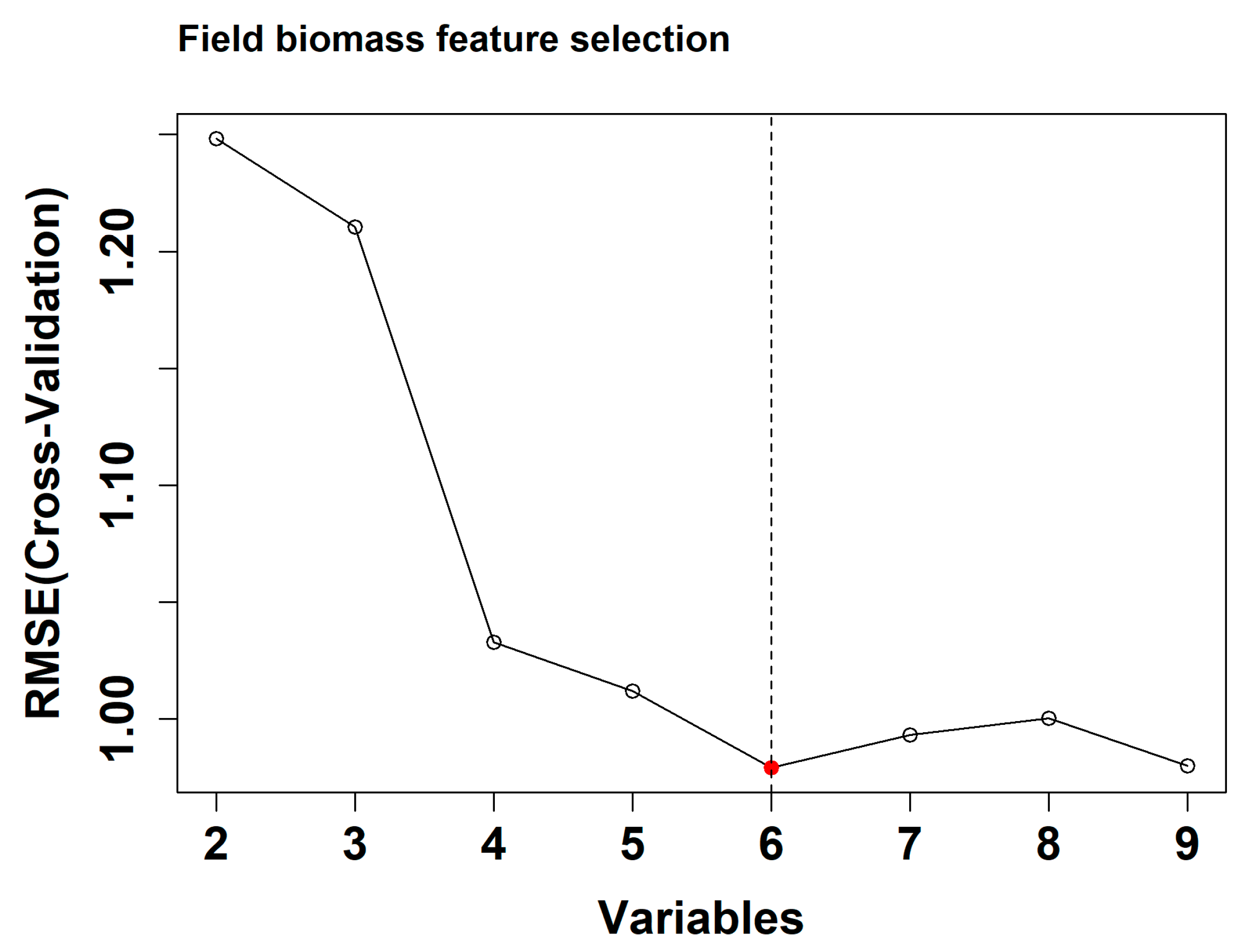
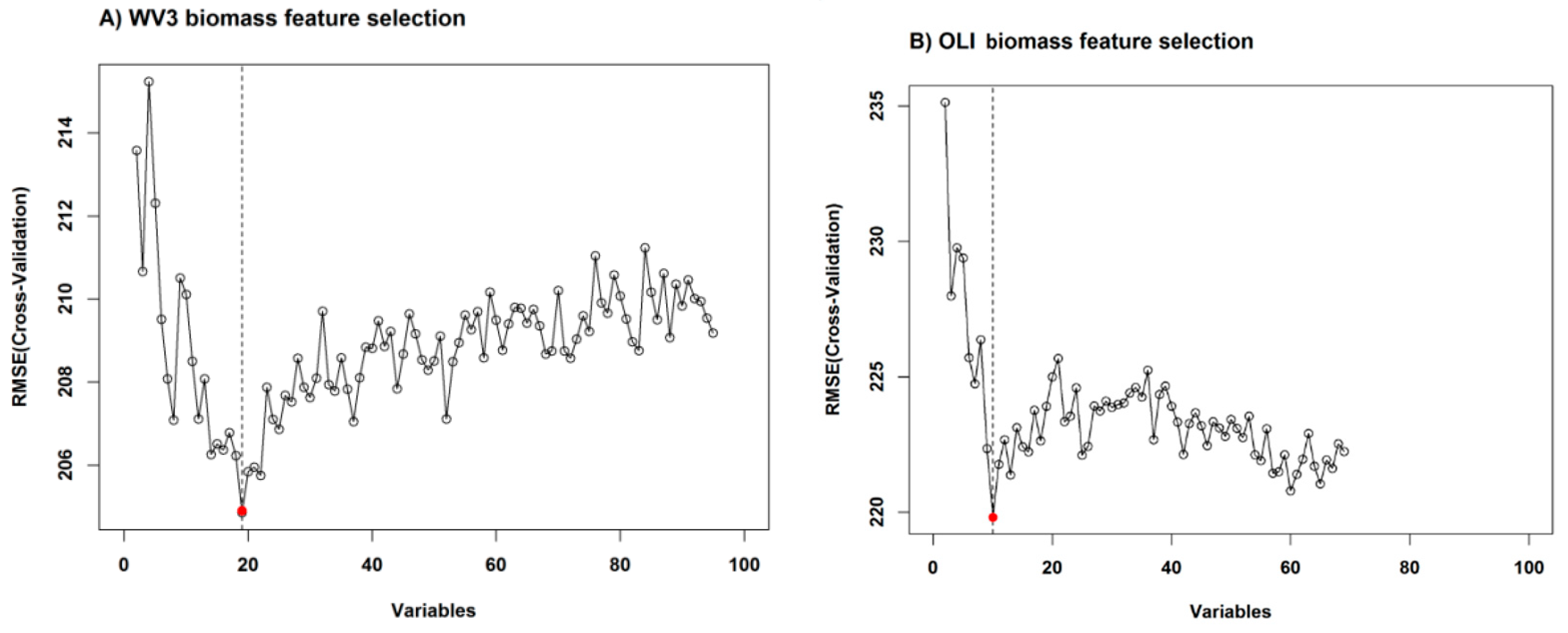
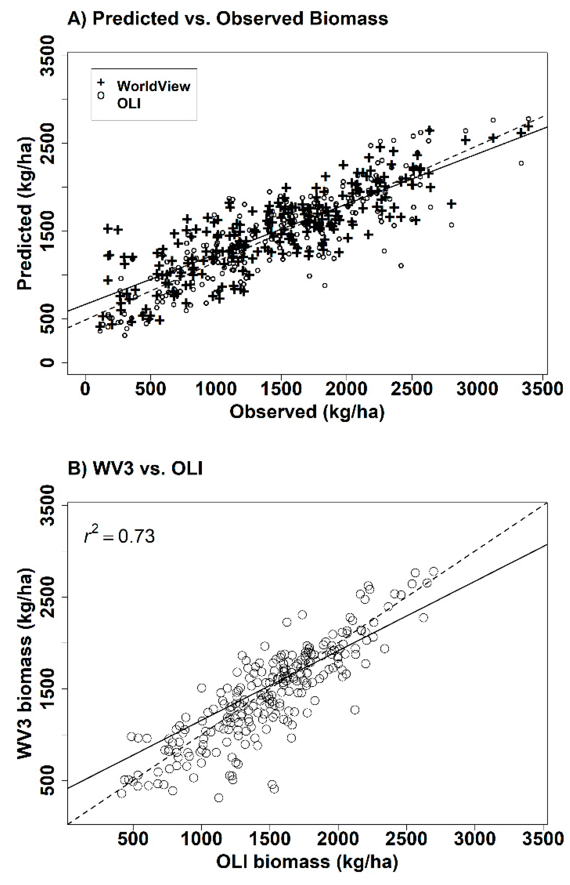
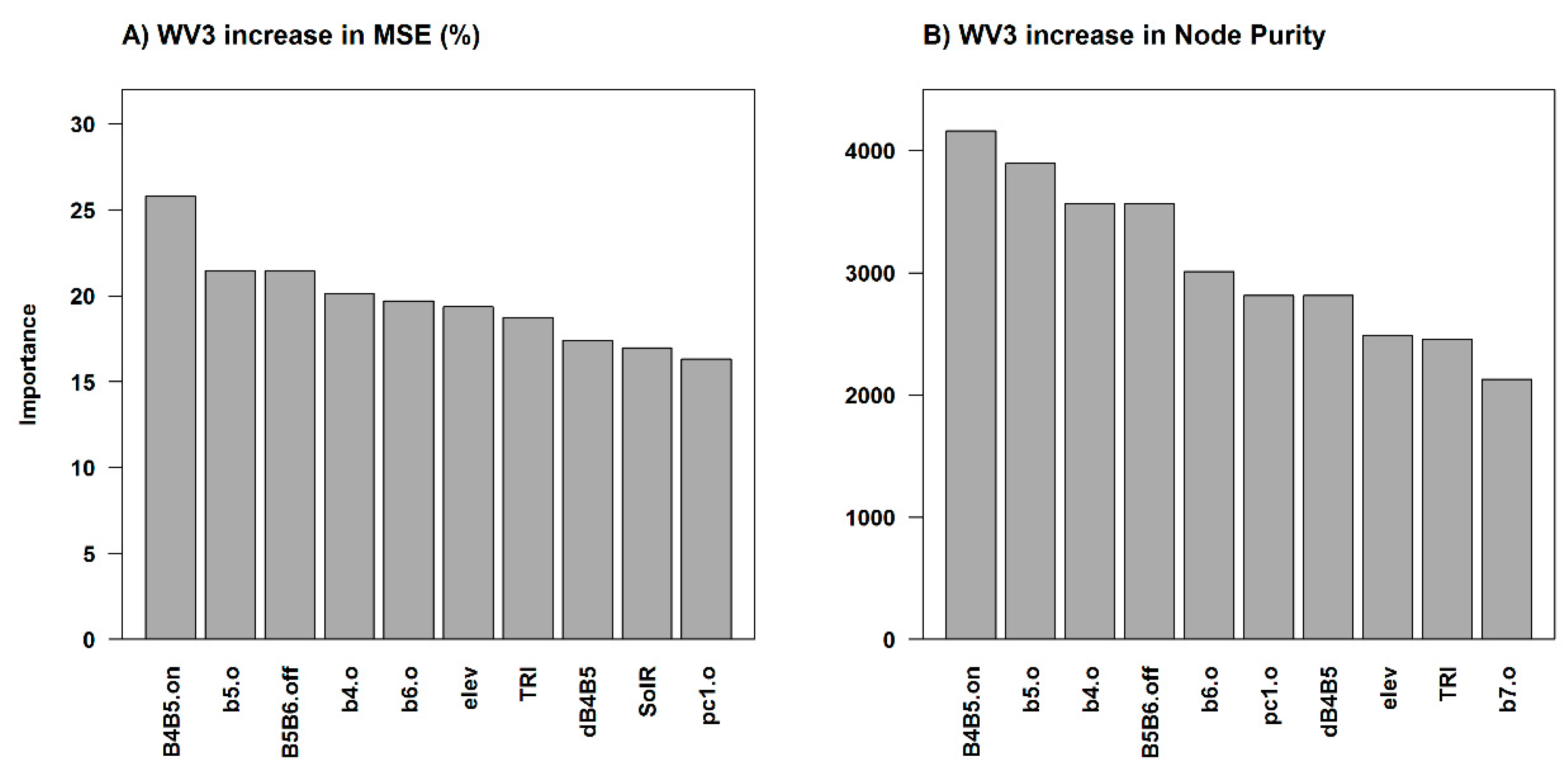
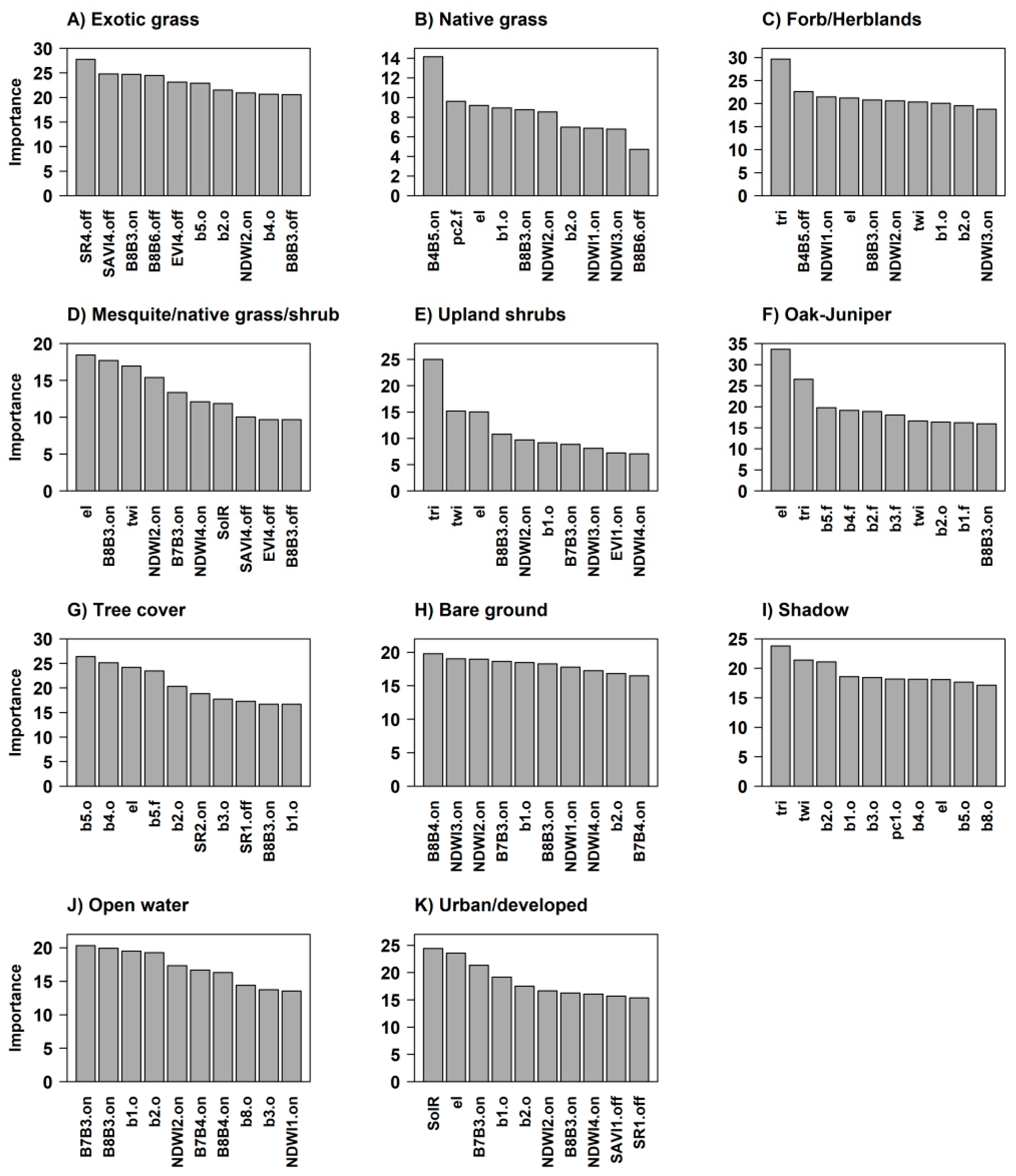
Table 1.
Spectral indices and layers used in creating the biomass and vegetation cover models using peak-green (leaf-on) and censed (leaf-off) vegetation Worldview-3 and Operational Land Imager satellite image dates. References supplied provide the general computational form and background information for each index and topographic variable.
| WV3 Indices | Spectral Channels/Equations | Reference |
|---|---|---|
| B4 & B5 | (ρband4 − ρband5)/(ρband4 + ρband5) | [55] |
| B7 & B3 | (ρband7 − ρband3)/(ρband7 + ρband3) | “ |
| B7 & B4 | (ρband7 − ρband4)/(ρband7 + ρband4) | “ |
| B7 & B5 | (ρband7 − ρband5)/(ρband7 + ρband5) | “ |
| B7 & B6 | (ρband7 − ρband6)/(ρband7 + ρband6) | “ |
| B8 & B3 | (ρband8 − ρband3)/(ρband7 + ρband3) | “ |
| B8 & B4 | (ρband8 − ρband4)/(ρband8 + ρband4) | “ |
| B8 & B5 | (ρband8 − ρband5)/(ρband8 + ρband5) | “ |
| B8 & B6 | (ρband8 − ρband6)/(ρband8 + ρband6) | “ |
| EVI1 | 1 G ∗ (ρband7 − ρband5)/(ρband7 + C1 ∗ ρband5 + C2 ∗ ρband2 + L) | [26] |
| EVI2 | G ∗ (ρband8 − ρband5)/(ρband8 + C1 ∗ ρband5 + C2 ∗ ρband2 + L) | “ |
| EVI3 | G ∗ (ρband7 − ρband6)/(ρband7 + C1 ∗ ρband6 + C2 ∗ ρband2 + L) | “ |
| EVI4 | G ∗ (ρband8 − ρband6)/(ρband8 + C1 ∗ ρband6 + C2 ∗ ρband2 + L) | “ |
| SAVI1 | 2 [(ρband7 − ρband5)/(ρband7 + ρband5 + L)] ∗ (1 + L) | [56] |
| SAVI2 | [(ρband8 − ρband5)/(ρband8 + ρband5 + L)] ∗ (1 + L) | “ |
| SAVI3 | [(ρband7 − ρband6)/(ρband7 + ρband6 + L)] ∗ (1 + L) | “ |
| SAVI4 | [(ρband8 − ρband6)/(ρband8 + ρband6 + L)] ∗ (1 + L) | “ |
| SR1 | ρband5/ρband7 | [57] |
| SR2 | ρband5/ρband8 | “ |
| SR3 | ρband6/ρband7 | “ |
| SR4 | ρband6/ρband8 | “ |
| NDWI1 | (ρband1 − ρband8)/(ρband1 + ρband8) | [58] |
| NDWI2 | (ρband2 − ρband8)/(ρband2 + ρband8) | “ |
| NDWI3 | (ρband1 − ρband7)/(ρband1 + ρband7) | “ |
| NDWI4 | (ρband2 − ρband7)/(ρband2 + ρband7) | ” |
| PC1 | Principal component 1 | [59] |
| PC2 | Principal component 2 | “ |
| OLI indices | ||
| B5 & B4 | (ρband5 − ρband4)/(ρband5 + ρband4) | [55] |
| B5 & B3 | (ρband5 − ρband3)/(ρband5 + ρband3) | “ |
| SAVI | 3 (ρband5 − ρband4)/(ρband5 + ρband4) + L ∗ (1 + L) | [56] |
| SATVI | (ρband5 − ρband3)/(ρband5 + ρband3 + L) ∗ (1 + L) − ρband7/2 | [30] |
| TVFC | SATVI − SATVImin/SATVImax − SATVImin ∗ 100 | “ |
| GCI1 | 4 (B5&B4 − μ/σ) − (TVFC − μ/σ) | [54] |
| GCI2 | (B5&B3 − μ/σ) − (TVFC − μ/σ) | “ |
| EVI | 5 G ∗ (ρband5 − ρband4)/(ρband5 + C1 ∗ ρband4 + C2 ∗ ρband2 + L) | [26] |
| SR | ρband4/ρband5 | [57] |
| NDWI1 | (ρband3 − ρband5)/(ρband3 + ρband5) | [58] |
| NDWI2 | (ρband3 − ρband6)/(ρband3 + ρband6) | “ |
| NDWI3 | (ρband3 − ρband7)/(ρband3 + ρband7) | “ |
| Terrain variables | ||
| Topographic Wetness Index | [60] | |
| Topographic Roughness Index | [61] | |
| Solar radiation | Globaltot = Dirtot + Diftot | [62] |
Note: 1 C1 = 6.0, C2 = 7.5, L = 1.0, 2 L = 0.5, 3 L = 0.5, 4 µ = VImean, σ = VIstd, 5 C1 = 6.0, C2 = 7.5, L = 1.0.
Table 2.
Land cover class descriptions and abbreviations used for mapping fuel-types on Buenos Aires National Wildlife Refuge (BANWR).
Table 2.
Land cover class descriptions and abbreviations used for mapping fuel-types on Buenos Aires National Wildlife Refuge (BANWR).
| Class name | Abbreviation | Description |
|---|---|---|
| Shadow | Sh | Image shadows from buildings, topography, trees and clouds |
| Tree cover | Tr | Lower elevation dense tree cover |
| Upland shrubs | Upsh | Upper elevation dense shrubs |
| Urban/developed | Ur | Roads, buildings and other human infrastructure |
| Open water | Wa | Tanks, ponds and perennial waters |
| Mesquite/native grass/shrub mix | Mgrw | Mixed mesquite trees, grass and shrubs |
| Bare ground | Ba | Rock, soil and other un-vegetated areas |
| Exotic grass | Xgr | Primarily Eroagrostis lemanniana |
| Forb and herblands | Fh | Dense herbaceous plants and forbs |
| Native grass | Ngr | Mainly sparse native grasses |
| Madrean oak–juniper | Oj | Upper elevation oak and juniper woodlands |
Table 3.
Random Forest percent cover model results from WV3 and OLI sensors with and without RFE predictor variable selection.
Table 3.
Random Forest percent cover model results from WV3 and OLI sensors with and without RFE predictor variable selection.
| Sensor | Cover Type | No. Variables | Var. Explained 1 | Features Selected | Var. Explained 2 | RMSE |
|---|---|---|---|---|---|---|
| WV3 | Herb | 90 | 42.6 | 27 | 49.1 | 14.8 |
| Woody | 90 | 25.7 | 30 | 31.1 | 10.7 | |
| Tree | 90 | 26.2 | 23 | 34.7 | 9.5 | |
| Bare ground | 90 | 47.3 | 21 | 54.9 | 9.9 | |
| OLI | Herb | 67 | 43.6 | 40 | 46.1 | 15.1 |
| Woody | 67 | 37.3 | 59 | 37.3 | 10.0 | |
| Tree | 67 | 43.5 | 61 | 45.3 | 8.4 | |
| Bare ground | 67 | 42.4 | 15 | 45.1 | 11.0 |
1 Amount of variance explained from Random Forest models without feature selection; 2 Amount of variance explained from optimized Random Forest models with feature selection.
Table 4.
Remote sensing based fine-fuel biomass (kg/ha) model results from Random Forest regression tree models with and without RFE predictor variable selection.
Table 4.
Remote sensing based fine-fuel biomass (kg/ha) model results from Random Forest regression tree models with and without RFE predictor variable selection.
| Sensor | Predictors 1 | No. Variables | Var. Explained 2 | RMSE | Features Selected | Var. Explained 3 | RMSE |
|---|---|---|---|---|---|---|---|
| WV3 | Spectral | 85 | 47.1 | 495.4 | 37 | 51.1 | 473.2 |
| Spectral and terrain | 90 | 51.1 | 462.8 | 37 | 56.6 | 438.8 | |
| Spectral, terrain and cover | 94 | 61.9 | 421.2 | 14 | 65.0 | 403.8 | |
| OLI | Spectral | 59 | 43.0 | 515.0 | 43 | 47.1 | 504.0 |
| Spectral and terrain | 67 | 45.5 | 503.6 | 64 | 48.9 | 493.2 | |
| Spectral, terrain and cover | 70 | 54.0 | 462.4 | 10 | 57.6 | 440.0 |
1 Three separate WV3 and OLI biomass models were developed using different sets of predictors; 2 Percentage of variance explained from Random Forest models without feature selection; 3 Amount of variance explained from optimized Random Forest models with feature selection.
Table 5.
Classification error matrices from (A) separate testing and training sample data and (B) all data bootstrapped error assessment using data left ‘out of bag’ (OOB) at each Random Forest classification model iteration.
Table 5.
Classification error matrices from (A) separate testing and training sample data and (B) all data bootstrapped error assessment using data left ‘out of bag’ (OOB) at each Random Forest classification model iteration.
| (A) | True | |||||||||||||
| Class | Ba | Xgr | Fh | Ngr | Oj | Mgrw | Sh | Tr | Upsh | Ur | Wa | Users acc. (%) | Producers acc. (%) | |
| Predicted | Ba | 42 | 0 | 0 | 0 | 0 | 0 | 0 | 1 | 0 | 4 | 0 | 89.4 | 95.5 |
| Xgr | 0 | 53 | 0 | 1 | 0 | 3 | 0 | 0 | 1 | 0 | 0 | 91.4 | 85.5 | |
| Fh | 0 | 1 | 18 | 0 | 0 | 0 | 0 | 1 | 0 | 0 | 0 | 90.0 | 72.0 | |
| Ngr | 1 | 4 | 1 | 2 | 0 | 1 | 0 | 0 | 0 | 0 | 0 | 22.2 | 22.2 | |
| Oj | 0 | 0 | 0 | 0 | 11 | 0 | 0 | 0 | 0 | 0 | 0 | 100.0 | 78.6 | |
| Mgrw | 0 | 4 | 5 | 6 | 0 | 20 | 0 | 4 | 1 | 0 | 0 | 50.0 | 83.3 | |
| Sh | 0 | 0 | 0 | 0 | 2 | 0 | 4 | 0 | 0 | 0 | 0 | 66.7 | 100.0 | |
| Tr | 0 | 0 | 1 | 0 | 1 | 0 | 0 | 25 | 0 | 0 | 0 | 92.6 | 80.6 | |
| Upsh | 0 | 0 | 0 | 0 | 0 | 0 | 0 | 0 | 2 | 0 | 0 | 100.0 | 50.0 | |
| Ur | 1 | 0 | 0 | 0 | 0 | 0 | 0 | 0 | 0 | 27 | 0 | 96.4 | 87.1 | |
| Wa | 0 | 0 | 0 | 0 | 0 | 0 | 0 | 0 | 0 | 0 | 12 | 100.0 | 100.0 | |
| Overall acc. % | 83.1 | |||||||||||||
| (B) | True | |||||||||||||
| Class | Ba | Xgr | Fh | Ngr | Oj | Mgrw | Sh | Tr | Upsh | Ur | Wa | Users acc. (%) | Producers acc. (%) | |
| Predicted | Ba | 170 | 0 | 1 | 0 | 0 | 1 | 0 | 0 | 0 | 11 | 0 | 92.9 | 89.5 |
| Xgr | 0 | 182 | 0 | 8 | 0 | 17 | 0 | 0 | 2 | 0 | 0 | 87.1 | 76.8 | |
| Fh | 0 | 0 | 60 | 1 | 0 | 13 | 0 | 3 | 0 | 0 | 0 | 77.9 | 80.0 | |
| Ngr | 0 | 23 | 3 | 15 | 0 | 24 | 0 | 0 | 0 | 0 | 0 | 23.1 | 48.4 | |
| Oj | 0 | 1 | 0 | 0 | 41 | 0 | 1 | 0 | 2 | 0 | 0 | 91.1 | 91.1 | |
| Mgrw | 2 | 24 | 8 | 7 | 0 | 69 | 0 | 7 | 0 | 0 | 0 | 59.0 | 50.0 | |
| Sh | 0 | 0 | 0 | 0 | 3 | 0 | 16 | 0 | 0 | 0 | 0 | 84.2 | 88.9 | |
| Tr | 1 | 0 | 3 | 0 | 0 | 9 | 1 | 95 | 0 | 2 | 0 | 85.6 | 87.2 | |
| Upsh | 0 | 7 | 0 | 0 | 1 | 5 | 0 | 3 | 9 | 0 | 0 | 36.0 | 69.2 | |
| Ur | 16 | 0 | 0 | 0 | 0 | 0 | 0 | 1 | 0 | 117 | 0 | 87.3 | 90.0 | |
| Wa | 1 | 0 | 0 | 0 | 0 | 0 | 0 | 0 | 0 | 0 | 54 | 98.2 | 100.0 | |
| Overall acc. % | 79.6 |
© 2018 by the authors. Licensee MDPI, Basel, Switzerland. This article is an open access article distributed under the terms and conditions of the Creative Commons Attribution (CC BY) license (http://creativecommons.org/licenses/by/4.0/).
Share and Cite
MDPI and ACS Style
Sesnie, S.E.; Eagleston, H.; Johnson, L.; Yurcich, E. In-Situ and Remote Sensing Platforms for Mapping Fine-Fuels and Fuel-Types in Sonoran Semi-Desert Grasslands. Remote Sens. 2018, 10, 1358. https://doi.org/10.3390/rs10091358
AMA Style
Sesnie SE, Eagleston H, Johnson L, Yurcich E. In-Situ and Remote Sensing Platforms for Mapping Fine-Fuels and Fuel-Types in Sonoran Semi-Desert Grasslands. Remote Sensing. 2018; 10(9):1358. https://doi.org/10.3390/rs10091358
Chicago/Turabian StyleSesnie, Steven E., Holly Eagleston, Lacrecia Johnson, and Emily Yurcich. 2018. "In-Situ and Remote Sensing Platforms for Mapping Fine-Fuels and Fuel-Types in Sonoran Semi-Desert Grasslands" Remote Sensing 10, no. 9: 1358. https://doi.org/10.3390/rs10091358
Note that from the first issue of 2016, this journal uses article numbers instead of page numbers. See further details here.