The Offset-Compensated Nonlocal Filtering of Interferometric Phase


1
DLR, German Aerospace Center, Münchner Straße 20, 82234 Weßling, Germany
2
DIETI, Università Federico II di Napoli, Via Claudio 21, 80125 Napoli, Italy
*
Author to whom correspondence should be addressed.
Remote Sens. 2018, 10(9), 1359; https://doi.org/10.3390/rs10091359
Submission received: 26 July 2018
/
Revised: 23 August 2018
/
Accepted: 25 August 2018
/
Published: 27 August 2018
(This article belongs to the Special Issue SAR in Big Data Era)
Abstract
:The nonlocal approach, proposed originally for additive white Gaussian noise image filtering, has rapidly gained popularity in many applicative fields and for a large variety of tasks. It has proven especially successful for the restoration of Synthetic Aperture Radar (SAR) images: single-look and multi-look amplitude images, multi-temporal stacks, polarimetric data. Recently, powerful nonlocal filters have been proposed also for Interferometric SAR (InSAR) data, with excellent results. Nonetheless, a severe decay of performance has been observed in regions characterized by a uniform phase gradient, which are relatively common in InSAR images, as they correspond to constant slope terrains. This inconvenience is ultimately due to the rare patch effect, the lack of suitable predictors for the target patch. In this paper, to address this problem, we propose the use of offset-compensated similarity measures in nonlocal filtering. With this approach, the set of candidate predictors is augmented by including patches that differ from the target only for a constant phase offset, which is automatically estimated and compensated. We develop offset-compensated versions of both basic nonlocal means and InSAR-Block-Matching 3D (BM3D), a state-of-the-art InSAR phase filter. Experiments on simulated images and real-world TanDEM-X SAR interferometric pairs prove the effectiveness of the proposed method.
1. Introduction
Synthetic Aperture Radar Interferometry (InSAR) is one of the most powerful tools to gather information on Earth’s topography and its deformation in time. It exploits two or more SAR images of the same region, acquired with some spatial and/or temporal diversity. Indeed, the phase difference between two SAR images, or interferometric phase, wrapped in the interval, bears information on the scene topography, which is eventually recovered by means of sophisticated phase unwrapping methods.
Unfortunately, SAR images are corrupted by intense noise, which makes it difficult to extract reliable information from them. This applies in particular to interferometric data which are affected by spatial and temporal decorrelation effects, associated with scattering changes in the signal backscattered at the different antennas and at the different acquisition times. It is therefore customary to adopt some forms of data restoration before phase unwrapping.
The simplest, and still widespread, solution consists in averaging the data in a rectangular window centered on the target (boxcar filtering). Despite its simplicity, boxcar filtering works very well in stationary areas of the image, as the sample average is the Maximum Likelihood (ML) estimator for the interferometric phase and coherence [1,2]. However, non-stationary areas abound in SAR interferograms, due to the scene topography or line-of-sight displacements in the imaged region, and they can be arguably considered the most valuable source of information for InSAR systems [3,4]. In such areas, boxcar filtering blends together heterogeneous data, resulting in a significant loss of resolution, and large phase and coherence estimation errors near signal discontinuities. This impairs strongly the subsequent phase unwrapping procedure that relies on both phase and coherence values [5].
A number of methods have been proposed in the literature to perform accurate phase filtering in the presence of non-stationary signals. The filters proposed by Lee et al. [6] and by Goldstein et al. [7] are among the most popular. They both adapt to the local fringe morphology, by working in the spatial and frequency domains, respectively. Subsequently, a number of improvements have been proposed both to the Lee filter [8,9,10,11] and to the Goldstein filter [12,13,14], aiming at a better adaptivity to the local signal geometry.
Another popular approach is to use wavelet transforms, to exploit their ability to analyze the signal in space and frequency. An early wavelet-based filter had been proposed in [15] where the interferometric phase noise was modeled in the complex domain. Other filters rely on the undecimated wavelet transform [16] and wavelet packets [17]. A common trait of all such filters is a good preservation of the spatial resolution. Other promising approaches, though not as widespread as the previous ones, use polynomial approximations [18], sparse coding and dictionary learning [19], and Bayesian estimation with a Markov Random Field (MRF) prior [20]. MRFs have also been used in [21] for joint filtering of SAR phase and amplitude.
A major trend of the last decade has been the use of nonlocal filtering for SAR data restoration. The potential of this approach was immediately clear since the seminal work of Buades et al. [22], where the Nonlocal Means (NLM) algorithm was proposed for the restoration of images corrupted by Additive White Gaussian Noise (AWGN). As the name suggests, the main novelty of nonlocal filtering consists of looking for the best predictors of the current target beyond its immediate proximity. Armed with a suitable patch-based similarity measure, the best predictors can be singled out in a large search window, or even the whole image. The self-similarity of natural images provides a theoretical basis for this approach to succeed in most situations of interest.
A huge number of contributes followed the NLM paper [22], not only for AWGN denoising but also for other tasks and applicative fields. In particular, nonlocal methods were soon adapted to SAR imagery, showing excellent results with all types of data, from amplitude images [23,24,25] to interferometric phase fields [26,27,28,29,30], polarimetric images [29,31,32], and multitemporal stacks [33,34,35,36,37]. Interested readers are referred to [38] for a recent review of the methods and ideas.
The first nonlocal filter for InSAR data [26] was an iterative version of Nonlocal Means. Predictors were selected based on a probabilistic criterion relying on both image intensities and interferometric phase values. Improvements were then proposed in [27], using pyramidal representations, and [28], relying on higher-order singular value decomposition. In [29] a unified framework was proposed, using an adaptive procedure for predictor selection to ensure a good preservation of image structures.
In [30,39] we have proposed InSAR-BM3D, a nonlocal method for InSAR phase filtering inspired to the nonlocal Block-Matching 3D (BM3D) algorithm [40], which blends the nonlocal approach with transform-domain shrinkage and Wiener filtering. Indeed, BM3D is still a state-of-the-art filter for AWGN denoising, and its multiplicative-noise version, SAR-BM3D [24], is one of the best filters for SAR despeckling. To deal with complex data, InSAR-BM3D filters separately the real and imaginary parts of the signal, obtained after a local decorrelating transform, by means of wavelet thresholding and empirical Wiener filtering. Experiments on both simulated and real-world phase images proved InSAR-BM3D to be very effective in terms of both objective distortion measures and perceived image quality.
Nonetheless, in the very same experiments, a clear performance decay was observed, for both InSAR-BM3D and other nonlocal filters, in regions characterized by a uniform phase gradient. Considering that such regions, corresponding to terrains with a locally uniform slope, abound in SAR interferograms, this is a relevant issue for nonlocal InSAR filtering methods. Based on preliminary analyses, we attribute this problem to the well-known “rare patch” effect [41]. For uncommon target patches, there are very few patches similar enough to work as good predictors, which leads to inaccurate (high variance) estimates. A possible solution is to enlarge the search area, possibly to the whole image, but complexity would become quickly unbearable.
Here, to address this problem, we propose the use of an offset-compensated patch similarity measure [39]. The core idea is to augment the set of predictors for a given target patch by including also all patches that differ from it only for a constant phase offset. Since, in uniform gradient areas, such a phase offset can be accurately estimated, this approach guarantees a wealth of new reliable estimators, thus obviating to the rare-patch problem. The proposed approach can be also regarded as a means to remove the effects of scene topography from the estimation. Under this point of view, some related work has recently appeared in the literature. In [42,43], assuming a DEM is available, the topography-related phase fringe pattern was removed before filtering. Other methods [14,44], instead, assumed a locally linear phase, estimated its fringe frequency, and removed the corresponding phase pattern. Contrary to these methods, we make no prior assumption, and rely exclusively on a suitable similarity measure. We implement this idea both in plain NLM, and in InSAR-BM3D, observing in both cases a significant performance improvement.
In the rest of the paper, we provide some background on nonlocal filtering for SAR interferograms (Section 2), describe the proposed approach and its implementation in nonlocal filters (Section 3), carry out experiments with both simulated and real-world data (Section 4), discuss the results (Section 5), and finally draw conclusions (Section 6).
2. Background
In this section we recall the basic concepts of nonlocal filtering, with special attention to the InSAR phase filtering problem, and formulate the signal model and notation that will be used in the rest of the paper.
2.1. Nonlocal Filtering
As the name suggests, nonlocal filtering aims at overcoming the limitations of conventional or “local” filters, which estimate the value of the target pixel based on the values of its neighbors. Let be the observed image, with the clean image and an additive noise component We consider an additive noise model, but the concepts are readily extended to other models. Focusing on linear filters, the estimate of the clean image at location p is obtained as a weighted average of noisy pixels
where p and q are spatial variables (we use single index for compactness), and a suitable window centered on p. For example, a space-invariant Gaussian filter has weights of the form
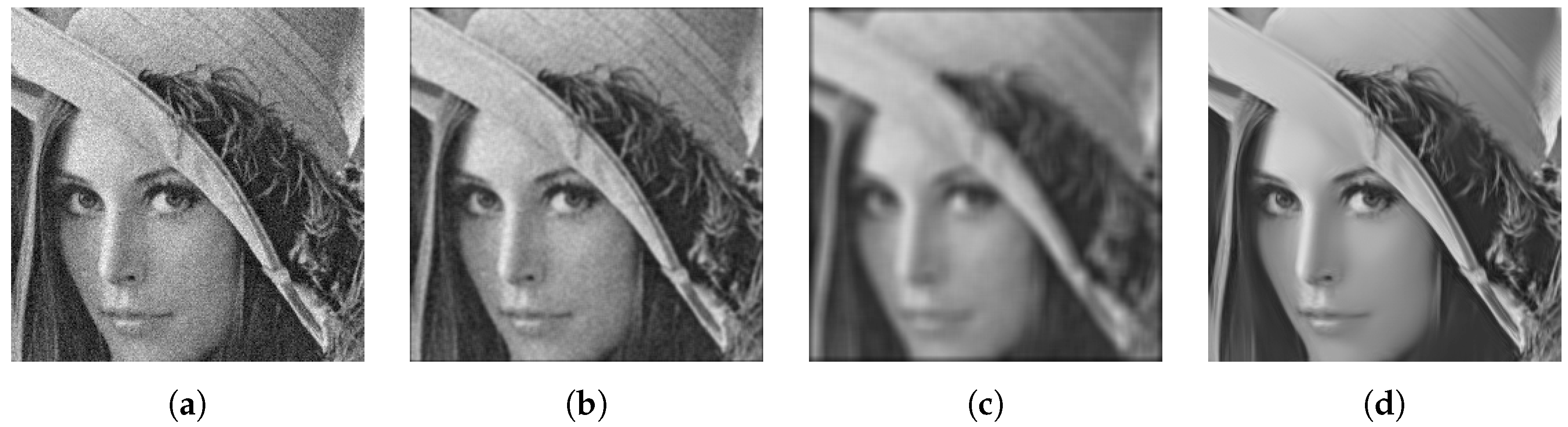
where is the spatial distance between locations p and q, C is a normalizing constant and a decay parameter. Therefore, a Gaussian filter relies mainly on pixels close to the target to estimate the clean value. Other local filters differ in the choice of weights, but still keep relying mostly on close neighbors of the target, often limited to a small window centered on the target itself. The underlying assumption is that close pixels are generally similar to one another. This certainly holds in stationary areas of the image, where, in fact, local filters work very well, reducing the noise variance without introducing any bias in the estimate. However, in non-stationary areas, like at the boundary between different regions, or in the presence of compact objects, close pixels are not necessarily similar, and local averages introduce significant biases in the estimate, which translates into a resolution loss. Figure 1 shows, for a sample noisy image (a), the output of boxcar filtering with a 3 × 3 (b), and a 9 × 9 (c) window, where the bias-variance trade-off appears clearly.
A large part of the recent denoising literature deals ultimately with this problem. The major breakthrough of nonlocal filtering is to abandon the underlying association between “close” and “similar”, and look for the best predictors without constraints. Accordingly, filtering is reformulated as a two-step procedure: (i) find the best predictors for the target pixel; (ii) estimate the clean value through a suitable average of the selected predictors. Of course, in this new paradigm the main issue becomes how to locate the best predictors in the whole image.
In their original paper [22], Buades et al. introduced the concept of the patch-based similarity measure, and proposed the nonlocal-means (NLM) algorithm. The weights of NLM have the same structure as in the Gaussian filter
with the difference that the spatial distance, , is replaced by an explicit estimate of signal dissimilarity . Since the true signal is not available, the dissimilarity is estimated on small blocks and of the observed signal centered on the target and predictor pixels, for example by the sum of squared errors, , which is optimal in the AWGN case. By using blocks, rather than individual pixels, one can reduce the impact of noise on dissimilarity estimation. Figure 1d shows the output of nonlocal means applied to the image of Figure 1a, where a large quality improvement appears w.r.t. local filters.
The nonlocal means paper has opened the way to intense work on nonlocal filtering, with a huge literature, including applications to SAR data filtering. Here, we only summarize, briefly, the BM3D algorithm, which is the basis of InSAR-BM3D [30] used in the rest of the paper.
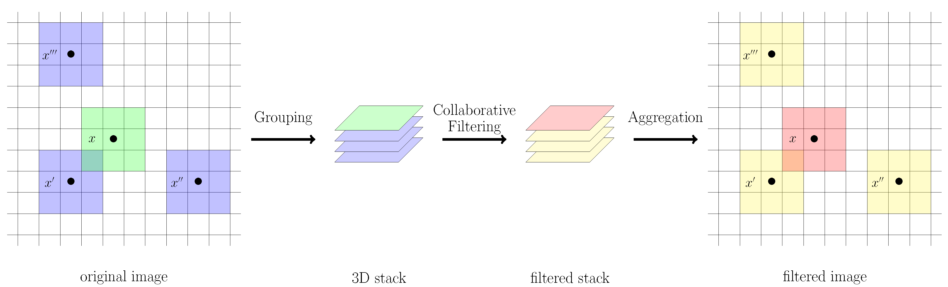
BM3D comprises three steps: grouping, collaborative filtering and aggregation, as shown graphically in Figure 2. In grouping, for each target block, a few similar blocks are singled out over a suitable search area, based on a block-similarity measure, and collected in a 3D stack. In the second step, these blocks are filtered jointly (that is, in a collaborative way) to exploit both local (intra-block) and nonlocal (inter-block) dependencies. Filtering is performed by transform-domain shrinkage, by applying a separable 3D wavelet transform to the stack, shrinking the transform coefficients to attenuate noise, and back-transforming the denoised stack. Finally, in the third step, the filtered blocks are returned to their original positions in the image, and overlapping blocks are aggregated to improve the estimation reliability.
A further significant difference with respect to basic NLM is the adoption of a two-pass filtering procedure. In the first pass, the noisy image, , is filtered as described above to produce a basic estimate, . This new image, however, is used only as a pilot to guide the second-pass filtering, which produces the final output, . The partially denoised pilot allows one to compute some key statistics for the wavelet shrinkage, and to compute more reliable similarity measures for the grouping phase, improving significantly the overall performance.
2.2. Signal Model
In our model [2,45], the interferometric pair is expressed for notational simplicity, here and in the following we drop spatial dependencies unless necessary. as the product of two standard circular Gaussian random variables with a suitable matrix T
where
depends only on the true amplitudes, and , interferometric phase, , and coherence, .
Accordingly, the observed complex interferogram, , can be regarded as a noisy version of the true interferogram, that is
where
depends on the true signal parameters, and n is a zero-mean signal-dependent noise term [46,47,48]
with covariance matrix
The terms on the main diagonal are the variances of the real and imaginary parts of the noise. In case of multi-looked data, the covariance matrix becomes simply , with L the number of looks.
2.3. InSAR Nonlocal Filtering
The application of the nonlocal means algorithm to InSAR data filtering is straightforward, we simply rewrite Equation (1) to estimate the true complex interferogram as
where p indicates the target pixel, and q its neighbors in the window , and the weights are computed according to the selected similarity measure. Note that NLM could be easily extended to estimate also the coherence and the signal amplitude. In this paper, however, we will focus only on the phase, and also, the similarity measure will rely only on phase information.
Although basic NLM is helpful to gain full insight into the main phenomena of interest, we will eventually focus on the state-of-the-art filter, InSAR-BM3D. At a very high level, InSAR-BM3D has the same algorithmic structure as BM3D. For each pixel, however, the grouping phase provides a couple of paired stacks, call them and , formed by blocks drawn from images and , respectively. These are used to compute a preliminary maximum-likelihood estimate of the local phase, , assumed to be constant over the block. The estimated phase is then used to decorrelate the real and imaginary parts of the interferogram. Such decorrelated components undergo collaborative filtering and aggregation, and are eventually processed to provide the filtered interferogram. A thorough description of the algorithm goes beyond the scope of this work, and we refer the reader to the original paper for more details.
3. Nonlocal Filtering with an Offset-Compensated Similarity Measure
As already said in the Introduction, we found experimentally that nonlocal filters work poorly on uniform gradient regions. Let us explain the nature of the problem by means of some synthetic examples, considering 1D signals and no noise, for the sake of simplicity. In Figure 3(left) we show, on the top row, a simple periodical signal, with a target patch highlighted in red. This signal may be representative of a mostly flat orography, with smooth variations. Nonlocal filters look for similar patches in the neighborhood of the target, so we plot, in the middle row, the distance between the target patch and all other patches. The plot clearly shows that a large number of similar patches exist, some very close to the target, some farther away. In the bottom plot, we highlight only the most similar patches (identical to the target in this zero noise example) but many more good predictors are available, leading eventually to a very reliable estimate. In Figure 3(right), instead, we consider a linear signal, representative of a constant slope orography. The distance plot in the middle row shows that only a few similar patches can be found, in the proximity of the target, some of which are highlighted in the bottom plot. With just a few predictors available, the variance of the estimate will grow significantly. These considerations are better substantiated in Appendix A where, considering a simplified setting, we compute the closed form of the Equivalent Number of Looks (ENL) for the nonlocal means filter in the presence of a constant slope signal.
However, going back to the example of Figure 3(left), it is clear that all patches in the neighborhood share with the target the very same shape, and they differ from it only for a constant term. Therefore, if we succeed in estimating this constant term, that is, its phase offset w.r.t. the target, then all patches can contribute to the estimate, with a predictable performance improvement. In other words, with a correct estimation and compensation of the phase offset, all regions with a constant phase slope would be re-conducted to the ideal case of flat terrain.
These synthetic examples are instrumental to explain our basic idea in simple terms. Of course, real-world images differ from such ideal cases under several respects, especially for (i) a more varied underlying signal, and (ii) the presence of noise. The random nature of the signal implies that, even after phase offset compensation, not all patches will be similar enough to the target to be good predictors. Moreover, with significant noise, estimating the phase offset may become itself a problem, leading to additional errors, in which case, costs and benefits should be carefully balanced.
In summary, our proposal can be summarized with the following points:
- for each phase patch in the neighborhood of the target, estimate the phase offset that minimizes the distance between the target patch and the offset-compensated predictor;
- perform nonlocal filtering with offset-compensated patches in place of the original patches.
Note that we do not specify the distance measure explicitly: any measure depending on phase differences can be replaced by its offset-compensated version. Likewise, any nonlocal filter can be implemented with this new measure in place of the original one. Here, we consider only the cosine distance, already used in [30] with good results, and implement the Offset-Compensated (OC) versions of NLM and InSAR-BM3D.
3.1. Cosine Dissimilarity
Let and be two size-N blocks of the interferometric phase image centered on pixels p and q, respectively.
We define the cosine dissimilarity between and as
Obviously, attains its minimum value, zero, when . Coherently with the above formula, we define the offset-compensated dissimilarity between and as
Now, we seek the minimizer of the quantity in square brackets, say , and the corresponding expression of . If we rewrite the dissimilarity as
with , the problem reduces to maximizing the latter summation. Now,
where
and indicates the phase of W. Of course, the maximum is obtained when , therefore
and, consequently
Note that the problem of Equations (12) and (13) is formulated in directional statistics [49] as the minimization of the dispersion of a circular variable, with sample , with respect to a value . The optimal solution of Equation (16) is called the mean direction of the data, in that context, while Equation (17) is the circular variance of the sample. Interestingly, the very same metric has been adopted is some recent papers concerning InSAR data filtering [50,51], although in a different context and with different aims.
Equation (17) can be now used to select the best predictors for the target patch, as in InSAR-BM3D, or to assign suitable weights to all patches in the analysis window, as in NLM and related methods. Actual filtering will then rely on the offset compensated patches, .
3.2. Preliminary Experiments with Offset-Compensated NLM
The impact of the proposed approach on state-of-the-art nonlocal filters, will be assessed in Section 4 with reference to the offset-compensated version of InSAR-BM3D.
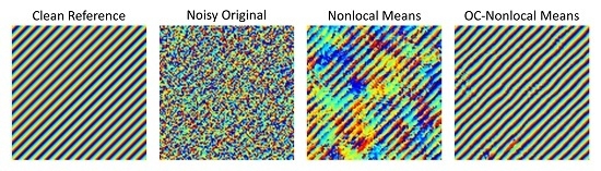
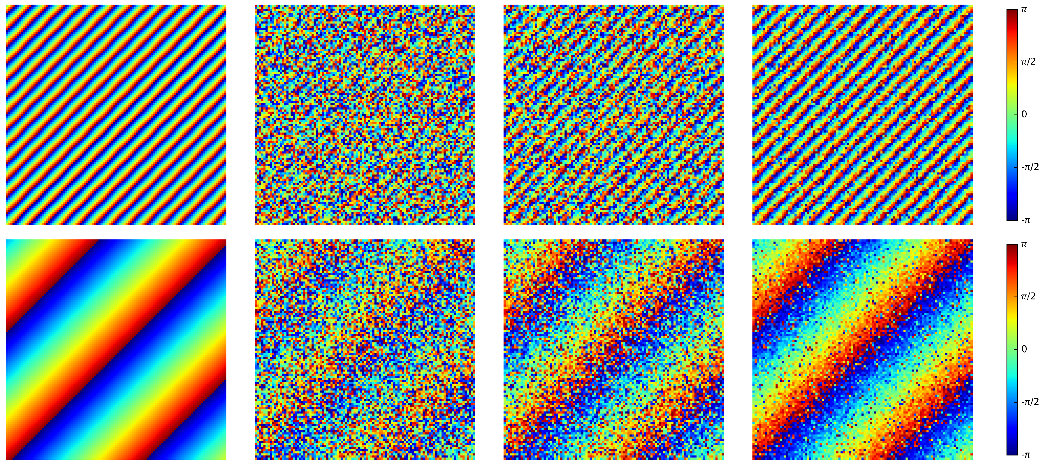
However, to better highlight some basic phenomena, we carried out some preliminary experiments with the much simpler OC-NLM. We wanted to understand how performance depends on noise intensity (hence coherence) and the local signal gradient. Therefore, we simulated simple test phase images, of a small size, 105 × 105 pixels, with constant coherence and phase gradient. In particular, we considered three levels of coherence, , 0.6, and 0.9, corresponding to high, medium, and low-intensity noise, and eight phase gradients with covering from a very fast-varying phase (to the limit of aliasing) to almost a constant phase. Figure 4 shows in false colors some of these test (wrapped) phase images, together with their ideal clean reference.
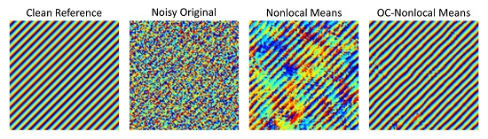
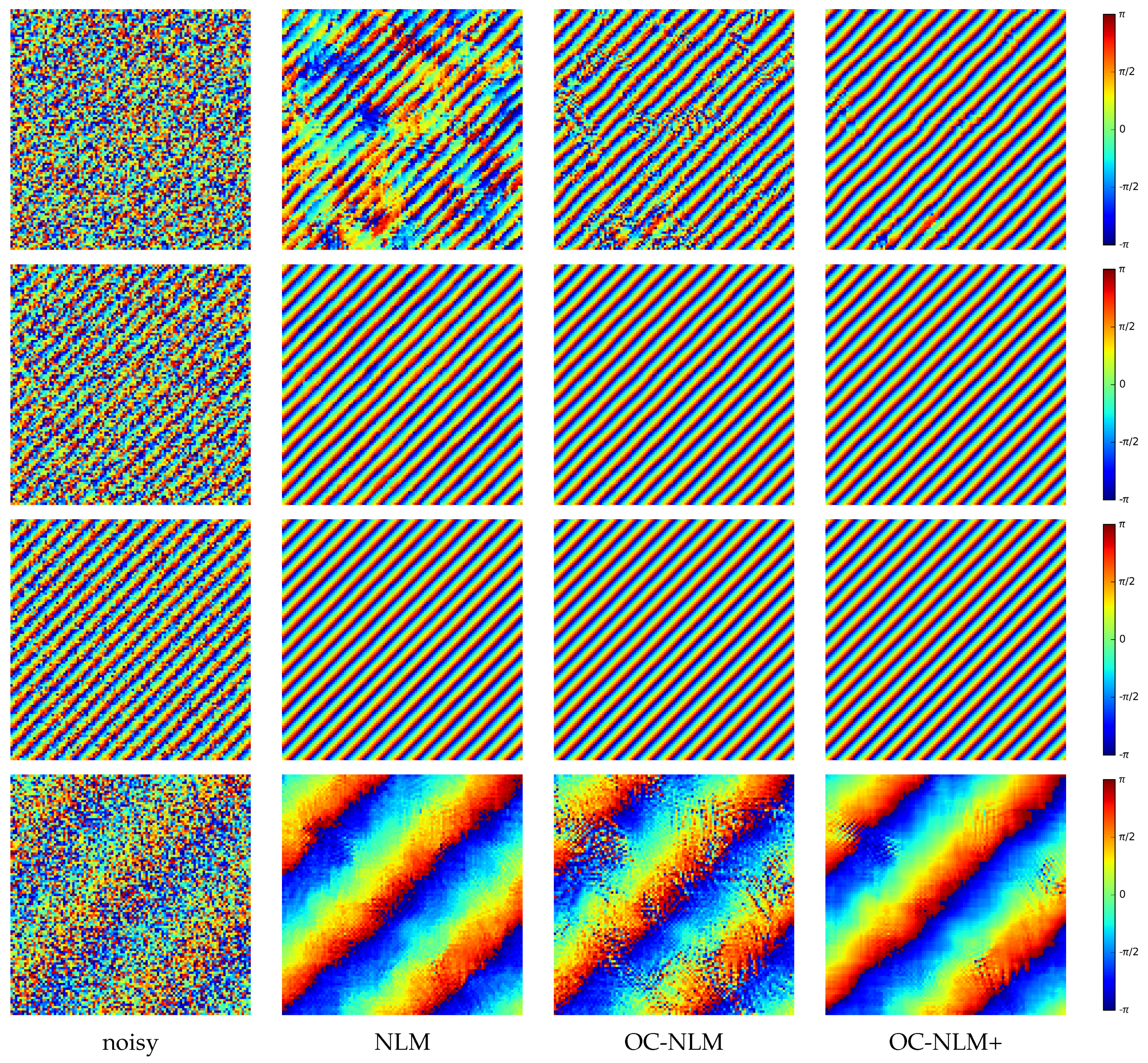
Figure 5, instead, compares the output of various NLM filters: basic NLM with cosine distance, the proposed offset-compensated version, OC-NLM, and a third adaptive version discussed later on. All versions use patches of 11 × 11 pixels, a search window of 21 × 21 pixels, and decay parameter . These values were selected by grid search through preliminary experiments on the synthetic test images described in Section 4. However, the minimum of the average error for the selected value of appears to be rather flat, hence non-critical. At low coherence and a large phase gradient (top row), basic NLM exhibits large errors, many phase fringes disappear throughout the image, and the overall structure of the phase is barely recognizable. The use of offset-compensated similarity grants a large performance improvement, allowing a good recovery of the general phase structure, although some significant errors keep appearing here and there. These are due to the intense noise affecting the original image. Although offset compensation provides a larger number of good predictors, the offset itself is not known in advance, and its wrong estimation introduces new errors. To reduce such errors, we consider a simple two-pass strategy similar to BM3D. The filtered phase obtained in the first pass is used in place of the original noisy phase to estimate the local offset in Equation (16) and the similarity measure in Equation (17). These quantities are then used to filter the noisy phase (not its first-pass estimate, to avoid drifts). This prefiltering strategy leads to a very good result, as visible in the rightmost figure. At medium coherence (second row) NLM works much better than before, and all phase fringes are correctly recovered although with significant local errors. Again, offset compensation grants some improvements, with near-perfect phase restoration, and prefiltering cannot improve further. Finally, at high coherence (third row) all versions of NLM work satisfactorily. In the bottom row, we show the interesting case of low coherence and low phase gradient. With such slow phase variations, there are plenty of good predictors in the neighborhood of the target, and NLM works already satisfactorily. On the contrary, due to errors in offset estimation, the OC version causes a clear performance impairment, which is only partially recovered thorough prefiltering. This observation confirms that on flat terrains, or in the presence of a small phase gradient, offset compensation is useless or even harmful and should not be used. To obtain the desired adaptivity to the local phase gradient, we compute the power spectrum of the signal in a small window centered on the target, and activate phase compensation only if a dominant peak exists at the medium-high frequencies.
A pseudo-code of the decision procedure is reported in Algorithm 1. Offset compensation is activated if the power spectrum peaks at medium-high frequencies (), and this peak is truly dominant, namely there is no comparable (within 10 dB) peak in the power spectrum far from the maximum (). While the first condition ensures that offset compensation is activated only in the presence of a significant slope, the second one reduces the risk to setting it on due to random noise fluctuations.
| Algorithm 1 OC-Switch. | |
| Require: | ▹ input patch, decision thresholds |
| Ensure: OC-switch | ▹ output on-off switch for offset compensation |
| 1: set OC-switch to OFF | |
| 2: | ▹ compute the power spectrum of |
| 3: | ▹ find the peak of G |
| 4: | ▹ distance of peak from origin, proxy for frequency |
| 5: | ▹ large-G region, within 10 dB of maximum |
| 6: | ▹ radius of large-G region |
| 7: if AND then | |
| 8: set OC-switch to ON | ▹ activate offset compensation |
| 9: end if | |
4. Experimental Results
We now focus on the offset-compensated version of InSAR-BM3D and analyze its performance on several simulated and real-world test images. Note that, except for the similarity measure, the OC version of InSAR-BM3D coincides with the basic algorithm, also because BM3D is already based on a two-pass strategy, and no prefiltering is necessary. In addition, offset compensation is applied only in areas where a significant phase gradient is estimated. With these premises, the reader is referred to [30] for any further detail.
In the experimental analysis we will compare results with some relevant methods, listed below.
The boxcar filter, has been included as a widespread and easily understood baseline, while the other reference methods can be arguably considered to be among the state of the art in this field. Together with the method acronym and the reference paper we recall the main parameters that can be set by the user. For all methods, these are set as suggested by the authors, or chosen to optimize the performance. Therefore, for example, in NL-InSAR we set the patch size to 7 × 7 pixels (dimPatch = 7) and the search area to 21 × 21 pixels (dimWindow = 21). Instead, for SpInPHASE we use dictionaries of both 256 and 512 atoms, choosing the best in each case. For InSAR-BM3D we used the default values. To ensure the reproducibility of results, the executable code of the proposed method and the simulated images used in the experiments will be available online at http://www.grip.unina.it/web-download.html.
4.1. Experiments on Simulated Data
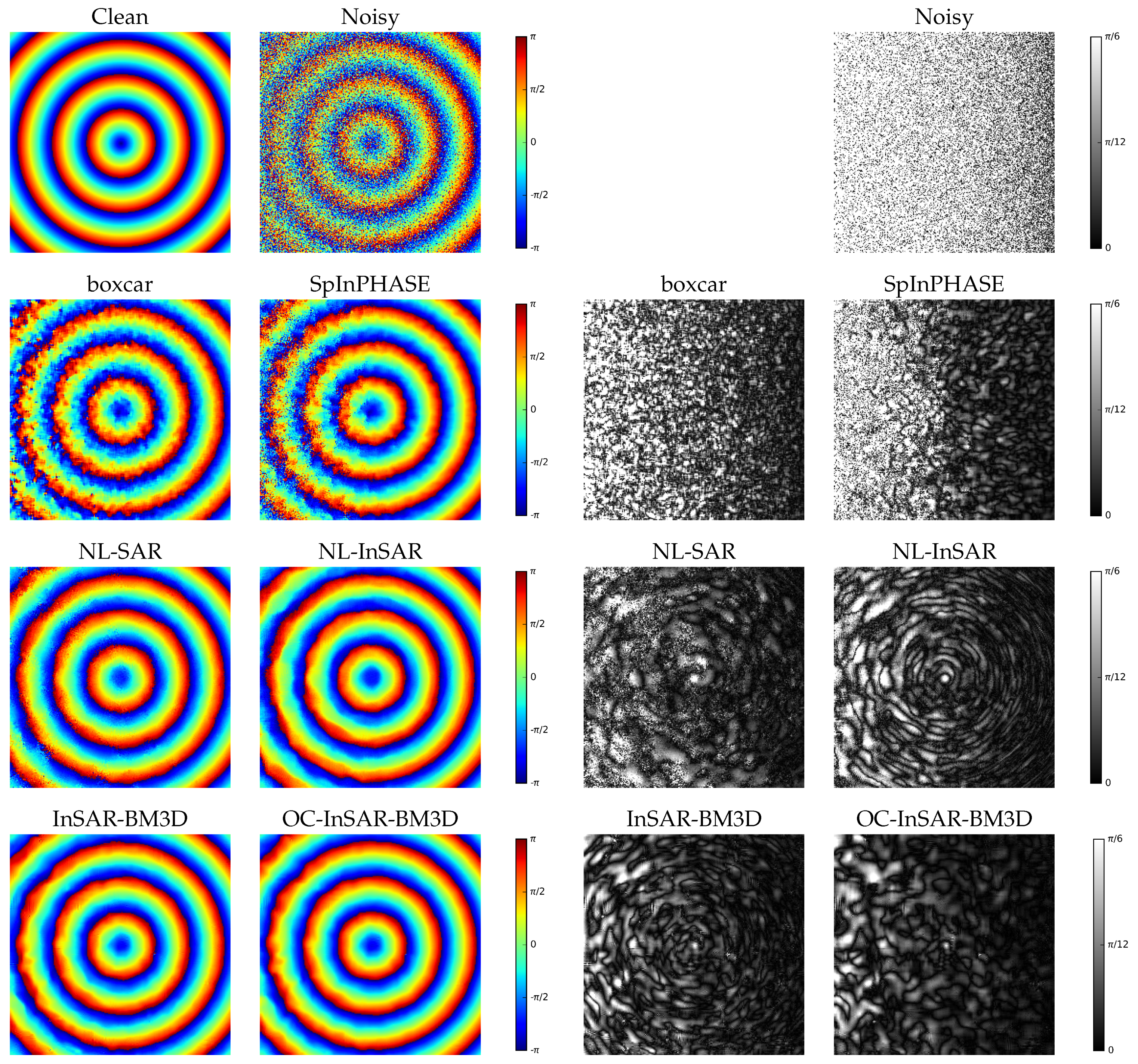
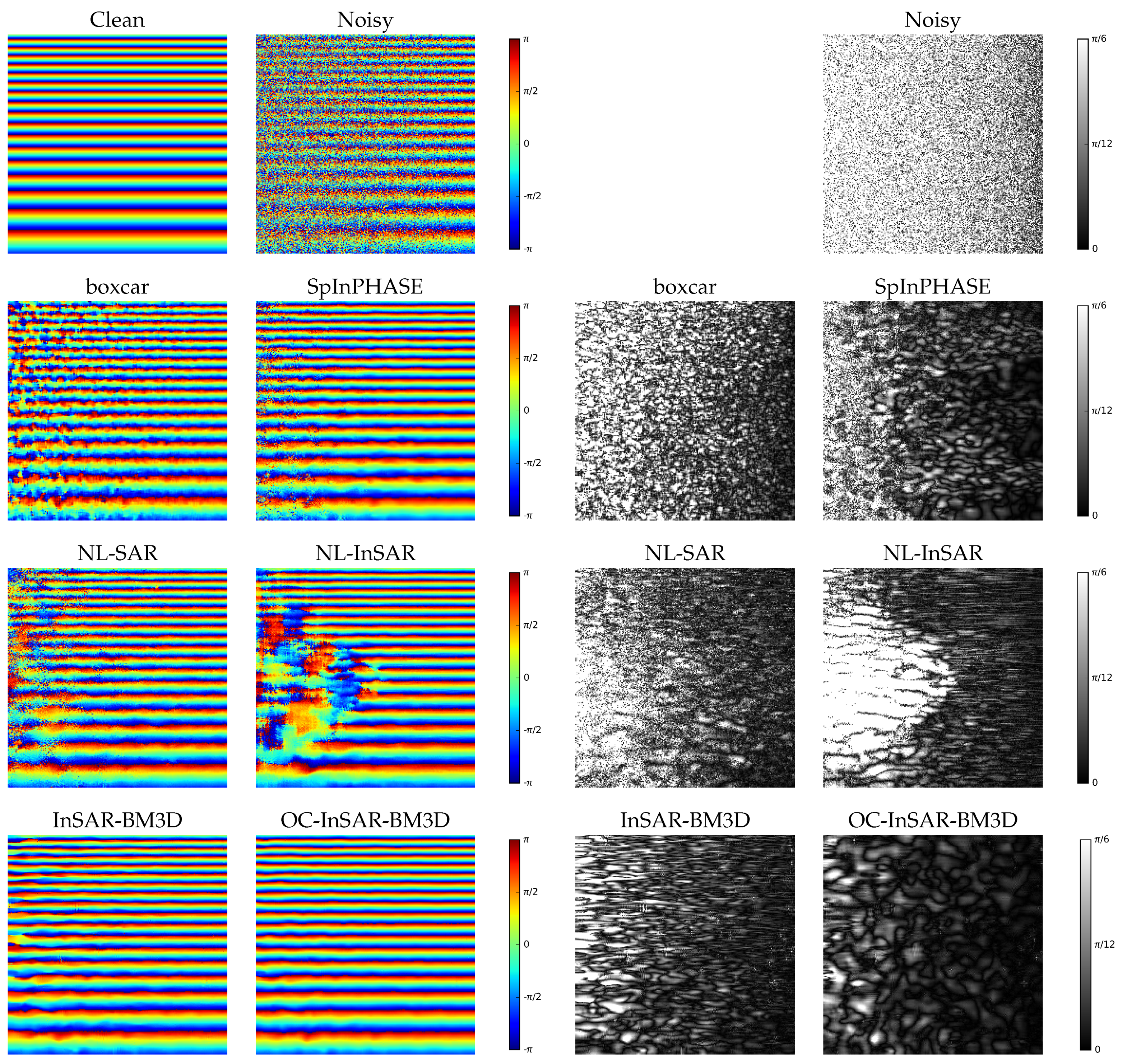
To carry out an objective assessment of performance in controlled conditions we use some simulated images, obtained by adding suitable synthetic noise on ideal phase fields. Images have size of 256 × 256 pixels and represent various realistic scenes: a Cone with circular symmetry and constant phase gradient along the radius, a Ramp with variable phase gradient, and fringe separation going from 28 to 8 pixels, and a richer image, Peaks, obtained by summing some Gaussian profiles, which simulates a more complex scenery with a varied geometry. Data are simulated by generating two circular complex standard Gaussian processes and correlating them through the matrix T in Equation (5).
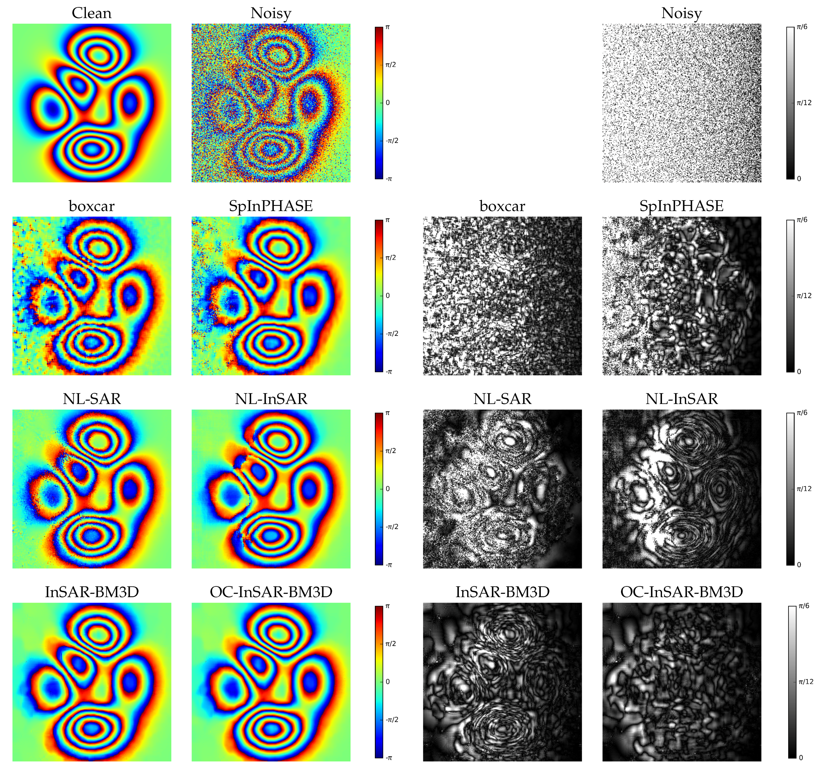
In order to gain insight into the dependence of filtering quality on phase noise intensity, the coherence grows linearly from left to right, from a minimum of 0.1 (very noisy) to a maximum of 0.9 (almost clean). Likewise, the amplitude grows from 21 to 255 digital numbers along the y axis, except for the ramp image (fixed amplitude) where the y axis is used to study the dependence on fringe frequency. In Figure 6, Figure 7 and Figure 8 we show, on the first row, the clean reference and the noisy version of the three test images, with the usual false-color representation in . It is clearly shown that the leftmost part of each image is extremely noisy, due to the very low coherence, and represents a very challenging testbed for all methods.
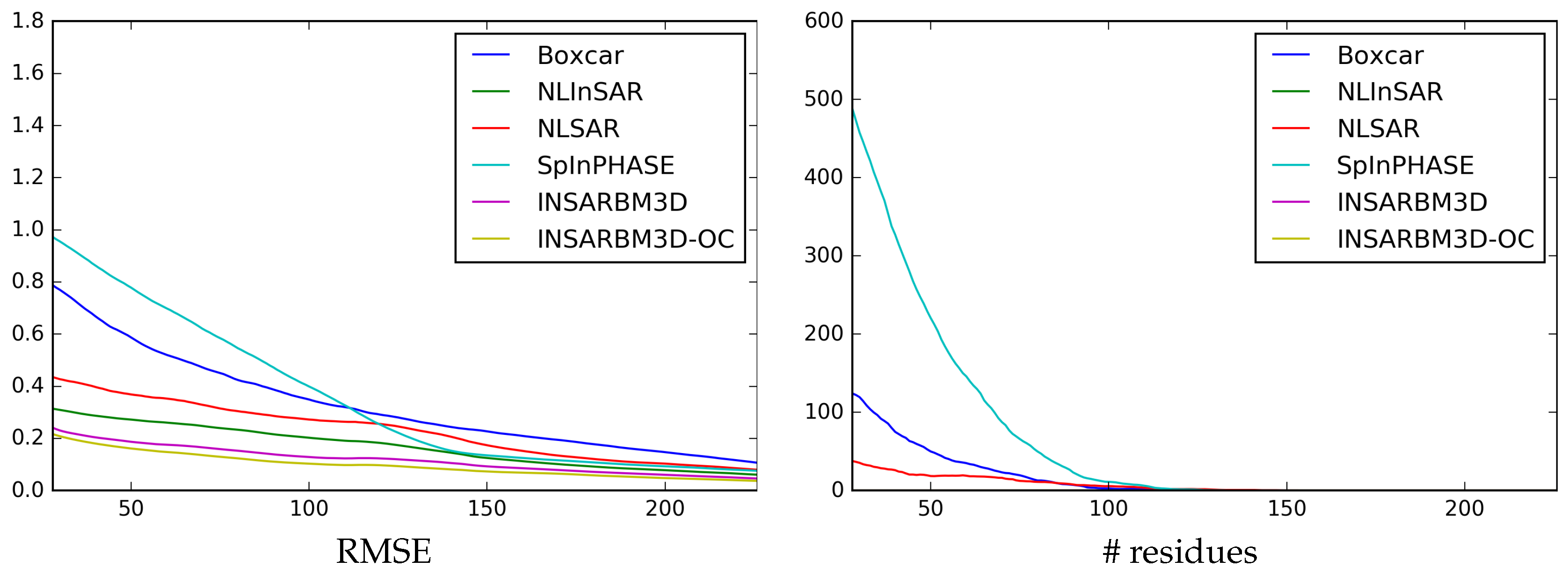
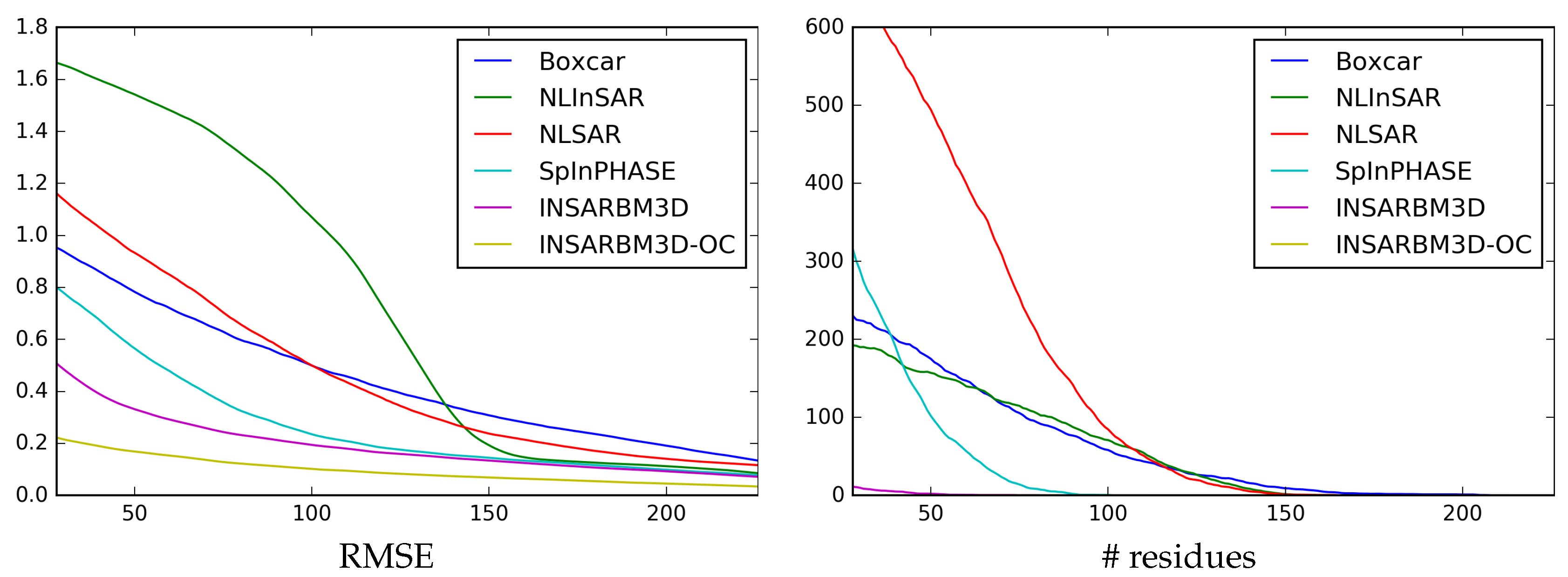
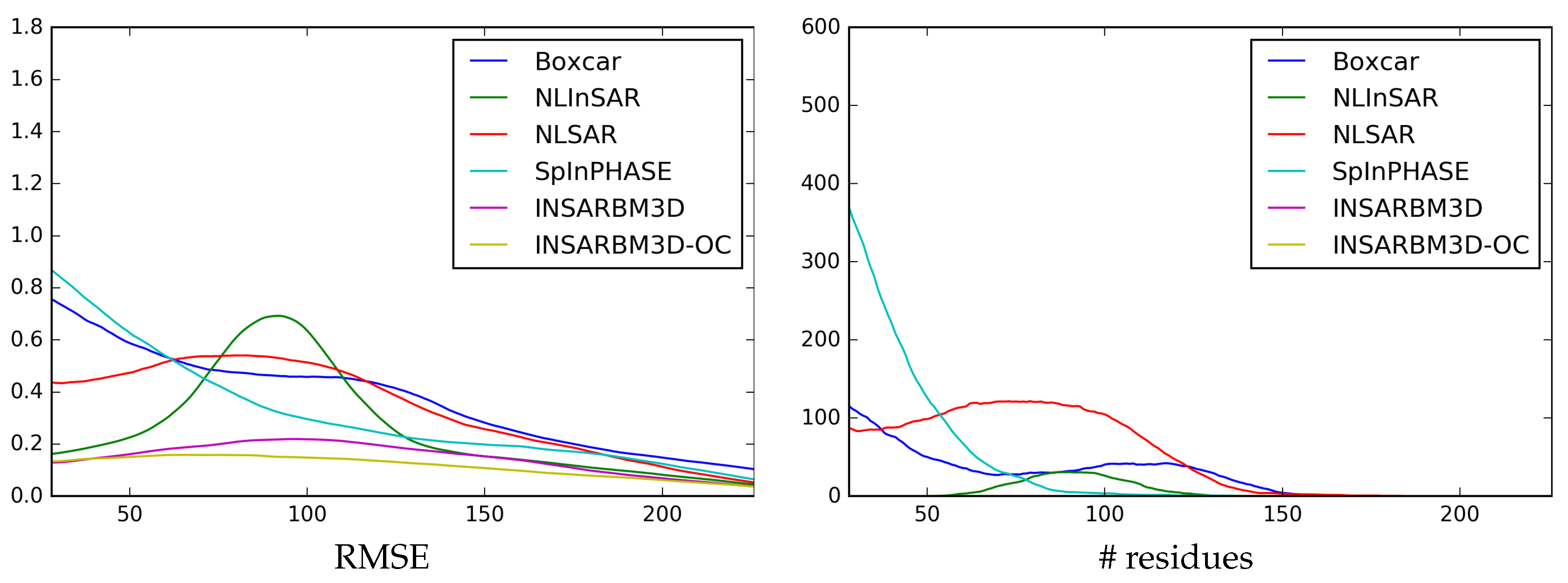
In Figure 6, Figure 7 and Figure 8 we also show, for all methods under test, the filtered images (left) and the difference between these and the clean references, called error images (right). Objective results, in terms of Root Mean-Square Error (RMSE) and number of residuesare instead reported in the graphs of Figure 9, Figure 10 and Figure 11. A residue is a singularity in the interferometric phase due to the presence of noise. The sum of increments of noiseless wrapped phases along a closed path is normally zero, and residues account for paths where this does not happen. Residues may heavily impair phase unwrapping. Hence, a good filter should reduce their number to allow reconstructing the interferometric phase structure. In order to study the dependence on noise intensity, these quantities are computed in sliding-window modality over vertical strips of width 32 pixels. Accordingly, the abscissa refers to the center pixel of the vertical strip, which goes from 28 to 226 to include only complete strips and avoid border effects. Therefore, for example, the RMSE decreases going from the left (low coherence) to the right (high coherence) part of each image. Finally, in Table 1 we report the RMSE and the number of residues computed over the whole image and averaged over ten repetitions of the experiment. The standard deviations, always quite small except for NL-SAR, are shown in parentheses and in smaller font.
Let us begin our analysis with Cone in Figure 6 and Figure 9. This is a rather smooth image, with a constant and limited phase gradient, the only challenge being the intense noise in the left part. Indeed, all methods work quite well on the right part, except for the well-known loss of resolution incurred by boxcar filtering. All phase fringes are accurately preserved and no residues are observed. Moving to the left noisy part, however, significant differences arise among the methods. NL-InSAR, InSAR-BM3D and OC-InSAR-BM3D keep providing a remarkably good result, with minor differences among them. NL-SAR performs slightly worse, with larger errors and the occurrence of some residues. As expected, the boxcar filter is not able to recover the correct phase fringes, in this area, and both performance indicators are impaired significantly. Instead, the sharp performance drop observed for SpInPHASE comes as a surprise, which removes only a small part of the noise and does not restore the true profile of the signal, introducing a large number of residues. The analysis of the error images reinforces such observations. Their global brightness level provides immediate insight into the RMSE. A more detailed analysis (it is recommended to observe the images suitably enlarged on a computer screen) provides further information about the structure of the error, easily revealing, for example, areas with residues. It is interesting to compare the error images of NL-InSAR, InSAR-BM3D and its OC version. The former two keep a clear circular structure, suggesting strong filtering interaction along the phase fringes. Such symmetries all but disappear in the latter, which we see as a proof that predictor patches are gathered more uniformly in the neighborhood of each target patch. The average performance indicators of Table 1 confirm that OC-InSAR-BM3D improves slightly over the plain version, and more significantly w.r.t. NL-InSAR and all other reference methods.
All above phenomena occur again, but much amplified, with ramp in, Figure 7 and Figure 10. In this image, in fact, there is a wide range of combinations of phase gradients and noise intensities, which highlights the critical cases due to the rare patch effect. A problematic region, corresponding to medium fringe frequencies and low coherence, emerges clearly in the NL-SAR and NL-InSAR filtered images. These methods, in fact, based on NLM, rely on the weighted average of all patches in the analysis window. However, in the critical region, there is a limited number of patches similar to the target, and they are extremely noisy, leading to the observed large errors. A larger number of good predictors is available both at lower fringe frequency (bottom part of the image) because of the smoother signal, while at higher fringe frequencies (upper part) multiple fringes fit in the analysis window. The impact on filtering quality is very strong: the signal profile is mostly lost, giving rise to large errors and a large number of residues. None of the other methods shows a similar behavior. Performance is impaired in the low coherence region, but rather uniformly over all fringe frequencies. Since the filtering task is more difficult than with Cone, a larger RMSE and a larger number of residues are observed on the average (see also Table 1) but the performance degradation is graceful. With this challenging image, OC-InSAR-BM3D ensures a significant performance improvement over the plain version, reaching ultimately about the same RMSE performance as with the Cone image. In addition, it shows no residues, a result not granted by InSAR-BM3D. Again, all the above considerations are largely confirmed by the analysis of the error images. The structural difference between the error images of InSAR-BM3D and OC-InSAR-BM3D are even more obvious, now, and the latter is uniformly darker, to indicate a lower RMSE.
Results for the Peaks image in Figure 8 and Figure 11, add little insight to the above analysis. NL-InSAR exhibits again some problems in large-gradient regions (see also the green curve in Figure 11) but such regions have a medium level of coherence, and hence the degradation is not catastrophic. In this case, offset compensation provides very limited gains. Actually, in the large flat regions in the outer parts of the image, the results of OC-InSAR-BM3D and InSAR-BM3D are exactly the same (see also the error image), because offset compensation is switched off altogether.
Table 1 summarizes the numerical results for all images and methods. InSAR-BM3D was already the top performer (at least on these synthetic images) and the adoption of offset compensation solves some residual problems in problematic regions. Interestingly, OC-InSAR-BM3D provides a remarkably uniform performance across the three images, in terms of both RMSE and # residues (always zero).
4.2. Experiments on Real-World Data
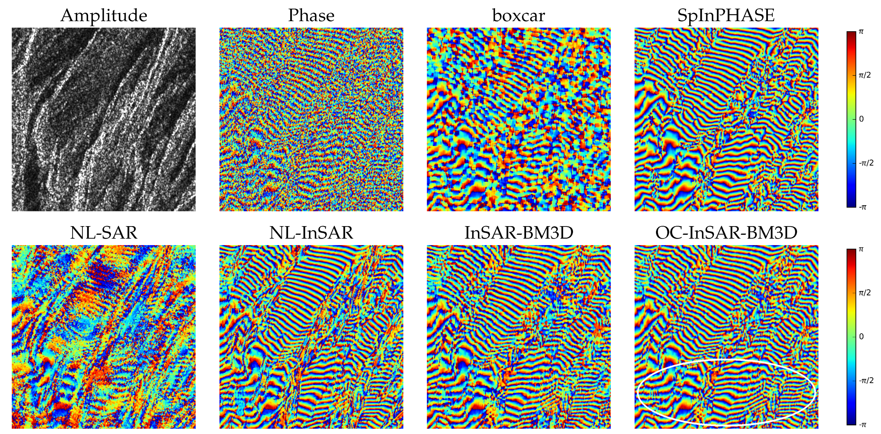
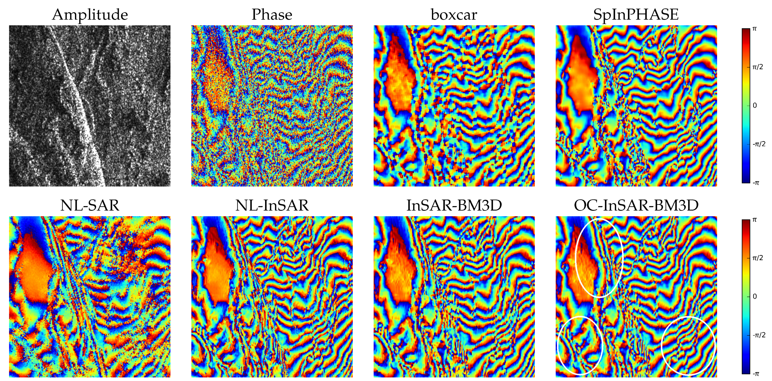
We conclude our analysis by considering a real-world scenario, a TanDEM-X interferometric pair acquired over the volcanic area of the Kamchatka region. This pair has been acquired in a bistatic configuration with a very large spatial baseline in order to achieve high sensitivity to height changes, i.e., high vertical resolution. In fact, it has a rather small height of ambiguity, 7 m, corresponding to the height difference for a single phase fringe. The large baseline causes significant decorrelation between the two interferometric acquisitions with the occurrence of generally denser fringe patterns in the interferometric phase. This is a typical example of the generation of high-resolution DEMs and hence an excellent testbed for assessing the capability of state-of-the-art filters. In Figure 12 and Figure 13 we show the amplitude and interferometric phase for two clips drawn from the Kamchatcka image, together with the filtering results from the six methods under comparison.
We chose an image that shares many characteristics with the simulated scenes considered before, therefore, not surprisingly, the results confirm most of the previous observations. The boxcar filter cannot work well on such high frequencies, and most phase fringes are lost or distorted through filtering, which may severely impair subsequent phase unwrapping. Furthermore, NL-SAR exhibits the problems highlighted with the Ramp image, uniformly on all clips. On the contrary, the performance gap among the remaining methods is now much reduced. This is especially surprising for SpInPHASE, which was one of worst performers on the simulated data. However, the RMSE graphs of Figure 9, Figure 10 and Figure 11 show for SpInPHASE a bimodal behavior: catastrophic at very low coherence and very competitive at high coherence. Since the Kamchatka image has a relatively high coherence, performance is mostly leveled. Nonetheless, a careful visual inspection reveals some significant differences, consistently in favor of OC-InSAR-BM3D, which is able to provide more regular phase patterns even in regions with very close fringes. To help the reader, we have highlighted with white ovals some regions where such differences can be more easily spotted.
4.3. Computational Performance
We computed the average running time of all algorithms on a 256 × 256 pixel image. Results must be taken with care, since the software is not homogeneous, with some codes written in C (NL-SAR and NL-InSAR) and others in MATLAB with some functions in C. Of course, the boxcar filter is by far the fastest, with a negligible running time. NL-SAR is also reasonably fast (20.3 s) significantly better than InSAR-BM3D (95.2 s) and NL-InSAR (105.0 s). SpInPHASE is much slower (457.8 s) due to the need to learn a dictionary. Finally, OC-InSAR-BM3D almost doubles the processing time w.r.t. the flat version (178.5), due to the additional processing steps.
5. Discussion
The experimental results confirm the potential of the proposed approach and make also clear its limits. Offset-compensated similarity improves results significantly in regions with a large phase gradient, especially at low coherence. This is especially clear with nonlocal means, in which case large improvements arise, but also with the state-of-the-art InSAR-BM3D. In the critical Ramp image, only the offset compensated version of InSAR-BM3D succeeds in preserving all phase fringes, whatever the slope, even in the very low-coherence region.
On the down side, in regions with a moderate phase gradient the performance may even be impaired, because the number of good predictors cannot be increased through offset compensation, while the estimate of the phase offset itself adds a new source of errors. For this reason, we propose an adaptive use of offset compensation, which is activated only in the presence of a significant phase slope. We also observe that, in the presence of a relatively high coherence, offset compensation does not provide significant improvements for state-of-the-art filters. On the other hand, at high coherence, improving phase filtering is not essential, because subsequent processes, like phase unwrapping, work already well. Effective and accurate filtering becomes important when the noise intensity is such that it impairs the performance of analysis methods, hence, at low coherence.
The goal of this study was to prove the potential of offset-compensated similarity in the context of InSAR phase filtering. Therefore, many topics that deserve further investigation were not considered in this first work. First, we focused on the cosine similarity measure, but the offset compensation concept may be easily applied to other measures as well. Moreover, these measures may take into account also amplitude and coherence to possibly improve performance and, of course, the aim of filtering can be also extended to the restoration of amplitude and coherence data themselves. Finally, offset-compensated versions of other nonlocal filters could be also developed and tested.
6. Conclusions
Nonlocal filtering methods suffer from the well-known rare patch effect. For uncommon signal patches, there is a scarcity of suitable predictor patches in the surrounding, which leads to low-quality restoration. This problem is especially relevant for InSAR phase filtering, because large regions of the image, characterized by a large phase gradient, and corresponding to areas with a constant slope, fit in the rare patch category. In such regions, even state-of-the-art nonlocal methods may provide poor results, with the filtered phase characterized by large errors and the presence of many residues.
In this paper, to deal with this problem, we proposed the use of offset-compensated similarity measures. For each candidate predictor patch, the mean phase offset w.r.t. the target patch was estimated and compensated for before computing similarity. By doing so, the pool of valid predictors can be significantly enlarged, allowing for a reliable estimate. Experiments on simulated and real-world data proved the validity of the approach.
Future work may explore the use of offset compensation with other similarity measures and the extension to other types of data and nonlocal filters.
Supplementary Materials
Software and implementation details will be made available online at http://www.grip.unina.it/ to ensure full reproducibility.
Author Contributions
All authors contributed to develop the method. F.S. and D.C. wrote the software code, and designed and performed the experiments; L.V. analyzed the related work, and contributed with F.S. and G.P. to write the paper; G.P. coordinated the activities.
Funding
This research received no external funding.
Conflicts of Interest
The authors declare no conflict of interest.
Appendix A. ENL of Nonlocal Means with Constant Slope Signals
In this Appendix we compute the equivalent number of looks (ENL) guaranteed by nonlocal means filtering in the presence of a constant-slope signal. The ENL provides information on the noise rejection ability of a filter in the presence of a stationary signal. However, for the sake of simplicity, we compute the weights in a continuous-space setting and in the absence of noise. Therefore, the resulting ENL cannot be assumed to accurately predict the performance of nonlocal means, let alone of more complex nonlocal filters. Nonetheless, it provides insight on the impact of signal slope on the filtering power of NLM.
Given the nature of the problem, we consider a one-dimensional continuous-space setting, with signal patches of length , and a search window of length . The target patch is placed at the origin, and the predictor patch at distance s from it. The signal is a linearly varying phase, , wrapped in . Patch dissimilarities are given by the mean square error (MSE). Specializing the NLM equations to these hypotheses, the weights write as
with the MSE between target and predictor patches. Initially, let us consider the geometry on the left part of Figure A1, with a moderate slope and hence no wrapping in the search window. In this case
and hence
The ENL depends on the distribution of the weights in the search window as follows
The integral at the numerator is
with and the Gaussian error function. Likewise, for the denominator,
with . Hence
For convenience, we normalize the ENL to its maximum, , attained for , and define the normalized slope , which counts the 2 cycles in the search window, obtaining eventually
This latter expression, however, holds only for the wrapping-free geometry of Figure A1(left), that is for . In the presence of wrapping, we can exploit the periodicity of the signal, see Figure A1(right), obtaining a more general expression, valid for all values of
with n an integer equal to . For all integer values of the same normalized ENL is obtained
which is also its asymptotic value.
To discuss these formulas, let us consider Figure A2 which shows the weights associated to candidate predictor patches as a function of their distance from the target patch. On the abscissa, we show the normalized distance from the target, , going from 0 (the target itself) to 1 (the search window limit). On the ordinate, the corresponding weights normalized to their maximum. Each subfigure corresponds to a different normalized slope, , while the curves in different colors correspond to different values of the decay parameter, . The first plot shows the flat signal case (), where all patches have the same weight, since all of them are good predictors, and the ENL is maximum. As the normalized slope increases, the number of effective predictors decreases more and more, and the ENL with it. When (second plot) there is already a scarcity of good predictors. A smaller (green) allows for the use of more predictors, although some of them are not really reliable, while larger values (blue, red) ensure a sharper selection. For (third plot) there are very few good predictors near the target while the farthest patches in the search window are bad predictors, with weights very close to 0. The trend continues with increasing slopes, like (last plot), however some good predictors appear farther away from the target, due to the periodicity of the wrapped phase, and the ENL tends to stabilize.
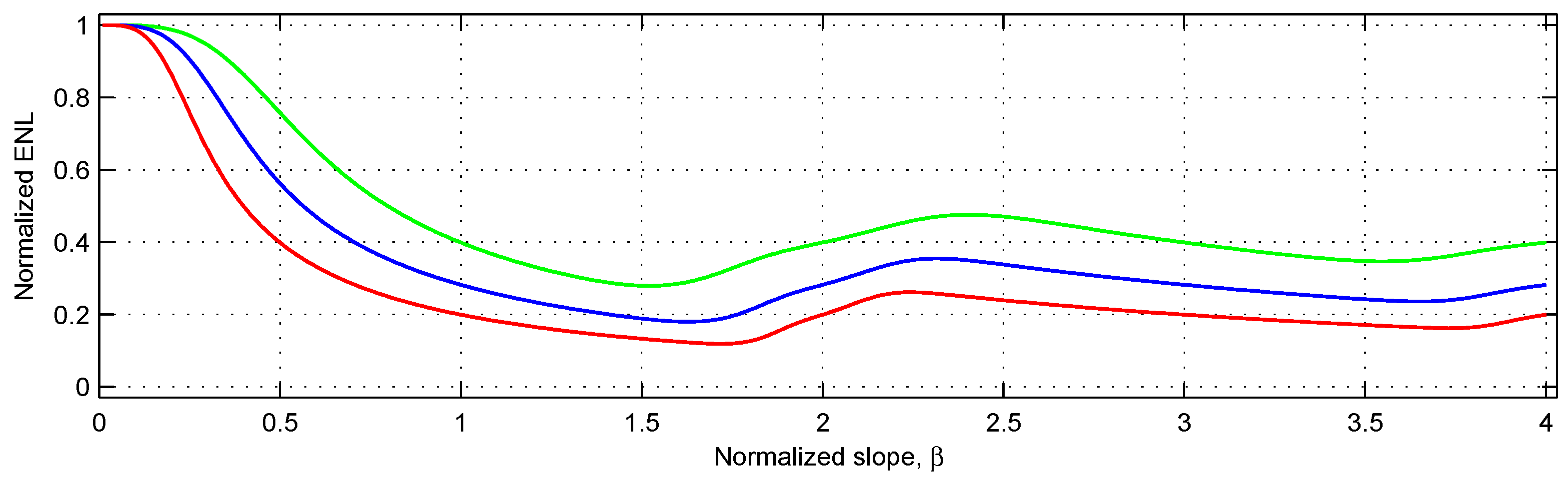
Figure A3 reports the ENL curves for the three values of used in Figure A2 and . At integer values of the computed ENL’s are approximately 0.4, 0.28, and 0.2.
Figure A1.
The 1d geometry used for ENL computation. Left: small slope, no phase wrapping in the search window. Right: large slope, and phase wrapping. Distances are normalized to the window search size. The target patch, at the center, is highlighted in red, a predictor patch in highlighted in black.

Figure A2.
Distribution of the normalized nonlocal means weights on the search window (only right half) as a function of phase slope and decay parameter. The four subfigures, from left to right, refer to the normalized slopes , , , . The three plots are for (green), (blue), (red).
Figure A2.
Distribution of the normalized nonlocal means weights on the search window (only right half) as a function of phase slope and decay parameter. The four subfigures, from left to right, refer to the normalized slopes , , , . The three plots are for (green), (blue), (red).

Figure A3.
Normalized ENL as a function of the normalized slope for three values of the decay parameter. The maximum is obtained for . For the ENL oscillates around the value obtained at integers, with decreasing amplitude of oscillations.
Figure A3.
Normalized ENL as a function of the normalized slope for three values of the decay parameter. The maximum is obtained for . For the ENL oscillates around the value obtained at integers, with decreasing amplitude of oscillations.

References
- Seymour, M.; Cumming, I. Maximum likelihood estimation for SAR interferometry. In Proceedings of the IEEE International Geoscience and Remote Sensing Symposium, Ottawa, ON, Canada, 8–12 August 1994; pp. 2272–2275. [Google Scholar]
- Bamler, R.; Hartl, P. Synthetic aperture radar interferometry. Inverse Probl. 1998, 14, R1–R54. [Google Scholar] [CrossRef]
- Zebker, H.; Villasenor, J. Decorrelation in interferometric radar echoes. IEEE Trans. Geosci. Remote Sens. 1992, 30, 950–959. [Google Scholar] [CrossRef] [Green Version]
- Massonnet, D.; Feigl, K. Radar interferometry and its application to changes in the Earth’s surface. Rev. Geophys. 1998, 36, 441–500. [Google Scholar] [CrossRef]
- Costantini, M. A novel phase unwrapping method based on network programming. IEEE Trans. Geosci. Remote Sens. 1998, 36, 813–821. [Google Scholar] [CrossRef]
- Lee, J.S.; Papathanassiou, K.; Ainsworth, T.; Grunes, M.; Reigber, A. A new technique for noise filtering of SAR interferometric phase images. IEEE Trans. Geosci. Remote Sens. 1998, 36, 1456–1465. [Google Scholar]
- Goldstein, R.; Werner, C. Radar interferogram filtering for geophysical applications. Geophys. Res. Lett. 1998, 25, 4035–4038. [Google Scholar] [CrossRef] [Green Version]
- Wu, N.; Feng, D.Z.; Li, J. A locally adaptive filter of interferometric phase images. IEEE Geosci. Remote Sens. Lett. 2006, 3, 73–77. [Google Scholar] [CrossRef]
- Fu, S.; Long, X.; Yang, X.; Yu, Q. Directionally adaptive filter for synthetic aperture radar interferometric phase images. IEEE Trans. Geosci. Remote Sens. 2013, 51, 552–559. [Google Scholar] [CrossRef]
- Chao, C.F.; Chen, K.S.; Lee, J.S. Refined filtering of interferometric phase from InSAR data. IEEE Trans. Geosci. Remote Sens. 2013, 51, 5315–5323. [Google Scholar] [CrossRef]
- Vasile, G.; Trouvé, E.; Lee, J.S.; Buzuloiu, V. Intensity-driven adaptive-neighborhood technique for polarimetric and interferometric SAR parameters estimation. IEEE Trans. Geosci. Remote Sens. 2006, 44, 1609–1621. [Google Scholar] [CrossRef] [Green Version]
- Baran, I.; Stewart, M.P.; Kampes, B.M.; Perski, Z.; Lilly, P. A modification to the Goldstein radar interferogram filter. IEEE Trans. Geosci. Remote Sens. 2003, 41, 2114–2118. [Google Scholar] [CrossRef]
- Song, R.; Guo, H.; Liu, G.; Perski, Z.; Fan, J. Improved Goldstein SAR interferogram filter based on empirical mode decomposition. IEEE Geosci. Remote Sens. Lett. 2014, 11, 399–403. [Google Scholar] [CrossRef]
- Jiang, M.; Dingi, X.; Li, Z.; Tian, X.; Zhu, W.; Wang, C.; Xu, B. The improvement for Baran phase filter derived from unbiased InSAR coherence. IEEE J. Sel. Top. Appl. Earth Observ. Remote Sens. 2014, 7, 3002–3010. [Google Scholar] [CrossRef]
- Lopez-Martinez, C.; Fabregas, X. Modeling and reduction of SAR interferometric phase noise in the wavelet domain. IEEE Trans. Geosci. Remote Sens. 2002, 40, 2553–2566. [Google Scholar] [CrossRef] [Green Version]
- Bian, Y.; Mercer, B. Interferometric SAR phase filtering in the wavelet domain using simultaneous detection and estimation. IEEE Trans. Geosci. Remote Sens. 2011, 49, 1396–1416. [Google Scholar] [CrossRef]
- Zha, X.; Fu, R.; Dai, Z.; Liu, B. Noise Reduction in Interferograms Using the Wavelet Packet Transform and Wiener Filtering. IEEE Geosci. Remote Sens. Lett. 2008, 5, 404–408. [Google Scholar]
- Bioucas-Dias, J.; Katkovnik, V.; Astola, J.; Egiazarian, K. Absolute phase estimation: adaptive local denoising and global unwrapping. Appl. Opt. 2008, 47, 5358–5369. [Google Scholar] [CrossRef] [PubMed]
- Hongxing, H.; Bioucas-Dias, J.M.; Katkovnik, V. Interferometric phase image estimation via sparse coding in the complex domain. IEEE Trans. Geosci. Remote Sens. 2015, 53, 2589–2602. [Google Scholar] [CrossRef]
- Ferraiuolo, G.; Poggi, G. A Bayesian filtering technique for SAR interferometric phase fields. IEEE Trans. Image Process. 2004, 13, 1368–1378. [Google Scholar] [CrossRef] [PubMed]
- Denis, L.; Tupin, F.; Darbon, J.; Sigelle, M. Joint regularization of phase and amplitude of InSAR data: Application to 3-D reconstruction. IEEE Trans. Geosci. Remote Sens. 2009, 47, 3774–3785. [Google Scholar] [CrossRef]
- Buades, A.; Coll, B.; Morel, J.M. A review of image denoising algorithms, with a new one. Multiscale Model. Simul. 2005, 4, 490–530. [Google Scholar] [CrossRef]
- Deledalle, C.A.; Denis, L.; Tupin, F. Iterative weighted maximum likelihood denoising with probabilistic patch-based weights. IEEE Trans. Image Process. 2009, 18, 2661–2672. [Google Scholar] [CrossRef] [PubMed]
- Parrilli, S.; Poderico, M.; Angelino, C.; Verdoliva, L. A nonlocal SAR image denoising algorithm based on LLMMSE wavelet shrinkage. IEEE Trans. Geosci. Remote Sens. 2012, 50, 606–616. [Google Scholar] [CrossRef]
- Cozzolino, D.; Parrilli, S.; Scarpa, G.; Poggi, G.; Verdoliva, L. Fast adaptive nonlocal SAR despeckling. IEEE Geosci. Remote Sens. Lett. 2014, 11, 524–528. [Google Scholar] [CrossRef]
- Deledalle, C.A.; Denis, L.; Tupin, F. NL-InSAR: Nonlocal interferogram estimation. IEEE Trans. Geosci. Remote Sens. 2011, 49, 1441–1452. [Google Scholar] [CrossRef]
- Chen, R.; Yu, W.; Wang, R.; Liu, G.; Shao, Y. Interferometric Phase Denoising by Pyramid Nonlocal Means Filter. IEEE Geosci. Remote Sens. Lett. 2013, 10, 826–830. [Google Scholar] [CrossRef]
- Lin, X.; Li, F.; Meng, D.; Hu, D.; Ding, C. Nonlocal SAR interferometric phase filtering through higher order singular value decomposition. IEEE Geosci. Remote Sens. Lett. 2015, 12, 806–810. [Google Scholar] [CrossRef]
- Deledalle, C.A.; Denis, L.; Tupin, F.; Reigber, A.; Jäger, M. NL-SAR: A unified nonlocal framework for resolution-preserving (Pol)(In) SAR denoising. IEEE Trans. Geosci. Remote Sens. 2015, 53, 2021–2038. [Google Scholar] [CrossRef]
- Sica, F.; Cozzolino, D.; Zhu, X.X.; Verdoliva, L.; Poggi, G. InSAR-BM3D: A Nonlocal Filter for SAR Interferometric Phase Restoration. IEEE Trans. Geosci. Remote Sens. 2018, 56, 3456–3467. [Google Scholar] [CrossRef]
- Chen, J.; Chen, Y.; An, W.; Cui, Y.; Yang, J. Nonlocal filtering for polarimetric SAR data: a pretest approach. IEEE Trans. Geosci. Remote Sens. 2011, 49, 1744–1754. [Google Scholar] [CrossRef]
- Hu, J.; Guo, R.; Zhu, X.; Baier, G.; Wang, Y. Non-local means filter for polarimetric SAR speckle reduction-experiments using TerraSAR-X data. In Proceedings of the ISPRS Annals of the Photogrammetry, Remote Sensing and Spatial Information Sciences, Taipei, Taiwan, 31 August–4 September 2015. [Google Scholar]
- Su, X.; Deledalle, C.; Tupin, F.; Sun, H. Two-step multitemporal nonlocal means for synthetic aperture radar images. IEEE Trans. Geosci. Remote Sens. 2014, 52, 6181–6196. [Google Scholar]
- Sica, F.; Reale, D.; Poggi, G.; Verdoliva, L.; Fornaro, G. Nonlocal adaptive multilooking in SAR multipass differential interferometry. IEEE J. Sel. Top. Appl. Earth Observ. Remote Sens. 2015, 8, 1727–1742. [Google Scholar] [CrossRef]
- Ferretti, A.; Fumagalli, A.; Novali, F.; Prati, C.; Rocca, F.; Rucci, A. A new algorithm for processing interferometric datastacks: SqueeSAR. IEEE Trans. Geosci. Remote Sens. 2011, 49, 3460–3470. [Google Scholar] [CrossRef]
- Fornaro, G.; Verde, S.; Reale, D.; Pauciullo, A. CAESAR: An approach based on covariance matrix decomposition to improve multibaseline-multitemporal interferometric SAR processing. IEEE Trans. Geosci. Remote Sens. 2015, 53, 2050–2065. [Google Scholar] [CrossRef]
- Chierchia, G.; El Gheche, M.; Scarpa, G.; Verdoliva, L. Multitemporal SAR image despeckling based on block-matching and collaborative filtering. IEEE Trans. Geosci. Remote Sens. 2017, 55, 5467–5480. [Google Scholar] [CrossRef]
- Deledalle, C.A.; Denis, L.; Poggi, G.; Tupin, F.; Verdoliva, L. Exploiting patch similarity for SAR image processing: the nonlocal paradigm. IEEE Signal Process. Mag. 2014, 31, 69–78. [Google Scholar] [CrossRef]
- Sica, F. Non-Local Methods for InSAR Parameters Estimation. Ph.D. Thesis, University of Naples Federico II, Napoli, Italy, 2016. [Google Scholar]
- Dabov, K.; Foi, A.; Katkovnik, V.; Egiazarian, K. Image denoising by sparse 3-D transform-domain collaborative filtering. IEEE Trans. Image Process. 2007, 16, 2080–2095. [Google Scholar] [CrossRef] [PubMed]
- Salmon, J.; Strozecki, Y. Patch reprojections for non-local methods. Signal Process. 2012, 92, 477–489. [Google Scholar] [CrossRef]
- Hagberg, J.O.; Ulander, L.M.; Askne, J. Repeat-pass SAR interferometry over forested terrain. IEEE Trans. Geosci. Remote Sens. 1995, 33, 331–340. [Google Scholar] [CrossRef]
- Touzi, R.; Lopes, A.; Bruniquel, J.; Vachon, P.W. Coherence estimation for SAR imagery. IEEE Trans. Geosci. Remote Sens. 1999, 37, 135–149. [Google Scholar] [CrossRef]
- Zebker, H.A.; Chen, K. Accurate estimation of correlation in InSAR observations. IEEE Trans. Geosci. Remote Sens. 2005, 2, 124–127. [Google Scholar] [CrossRef]
- Goodman, N. Statistical analysis based on a certain multivariate complex Gaussian distribution (an introduction). Ann. Math. Stat. 1963, 3, 152–177. [Google Scholar] [CrossRef]
- Just, D.; Bamler, R. Phase statistics of interferograms with applications to synthetic aperture radar. Appl. Opt. 1994, 33, 4361–4368. [Google Scholar] [CrossRef] [PubMed]
- Lee, J.S.; Hoppel, K.; Mango, S.; Miller, A. Intensity and phase statistics of multilook polarimetric and interferometric SAR imagery. IEEE Trans. Geosci. Remote Sens. 1994, 32, 1017–1028. [Google Scholar]
- Lopez-Martinez, C.; Pottier, E. On the extension of multidimensional speckle noise model from single-look to multilook SAR imagery. IEEE Trans. Geosci. Remote Sens. 2007, 45, 305–320. [Google Scholar] [CrossRef]
- Mardia, K.V.; Jupp, P.E. Directional Statistics; John Wiley & Sons: Hoboken, NJ, USA, 2000. [Google Scholar]
- Pepe, A.; Yang, Y.; Manzo, M.; Lanari, R. Improved EMCF-SBAS processing chain based on advanced techniques for the noise-filtering and selection of small baseline multi-look DInSAR interferograms. IEEE Trans. Geosci. Remote Sens. 2015, 53, 4394–4417. [Google Scholar] [CrossRef]
- Pepe, A.; Mastro, P. On the use of directional statistics for the adaptive spatial multi-looking of sequences of differential SAR interferograms. In Proceedings of the IEEE International Geoscience and Remote Sensing Symposium 2017, Fort Worth, TX, USA, 23–28 July 2017; Volume 2, pp. 3791–3794. [Google Scholar]
Figure 1.
Bias-variance trade-off and nonlocal filtering. From left to right: original noisy image, output of 3 × 3 boxcar filter, output of 9 × 9 boxcar filter and output of nonlocal means.
Figure 1.
Bias-variance trade-off and nonlocal filtering. From left to right: original noisy image, output of 3 × 3 boxcar filter, output of 9 × 9 boxcar filter and output of nonlocal means.

Figure 2.
Main conceptual steps of BM3D filtering.

Figure 3.
Two synthetic examples to motivate the need for offset-compensated similarity measures. Top: simple noiseless signals, characterized by small fluctuations (left), or a constant gradient (right). Middle: squared error between the local patch and the target (red) patch. Bottom: patches (black) similar to the target are rare in the presence of a significant gradient. Many more would be available with offset compensation.

Figure 4.
Examples of test phase images (size 105 × 105 pixels), used in the preliminary experiments. From top to bottom: large (), and medium phase gradient (). From left to right: clean image, noisy images at low (), medium (), and high () coherence.
Figure 4.
Examples of test phase images (size 105 × 105 pixels), used in the preliminary experiments. From top to bottom: large (), and medium phase gradient (). From left to right: clean image, noisy images at low (), medium (), and high () coherence.

Figure 5.
Sample filtering results with various versions of NLM. From top to bottom: large gradient-low coherence, large gradient-medium coherence, large gradient-high coherence, medium gradient-low coherence. From left to right: noisy original, filtered with NLM, OC-NLM, prefiltered adaptive OC-NLM.

Figure 6.
Cone image (top). Filtered images (left) and error images (right) for all methods under comparison.
Figure 6.
Cone image (top). Filtered images (left) and error images (right) for all methods under comparison.

Figure 7.
Ramp image (top). Filtered images (left) and error images (right) for all methods under comparison.
Figure 7.
Ramp image (top). Filtered images (left) and error images (right) for all methods under comparison.

Figure 8.
Peaks image (top). Filtered images (left) and error images (right) for all methods under comparison.
Figure 8.
Peaks image (top). Filtered images (left) and error images (right) for all methods under comparison.

Figure 9.
Cone image. Sliding-window RMSE (left) and residues (right) for all methods under comparison.
Figure 9.
Cone image. Sliding-window RMSE (left) and residues (right) for all methods under comparison.

Figure 10.
Ramp image. Sliding-window RMSE (left) and residues (right) for all methods under comparison.
Figure 10.
Ramp image. Sliding-window RMSE (left) and residues (right) for all methods under comparison.

Figure 11.
Peaks image. Sliding-window RMSE (left) and residues (right) for all methods under comparison.
Figure 11.
Peaks image. Sliding-window RMSE (left) and residues (right) for all methods under comparison.

Figure 12.
Kamchatka Clip #1. Filtered (right) and method noise images (left) for all methods under comparison.
Figure 12.
Kamchatka Clip #1. Filtered (right) and method noise images (left) for all methods under comparison.

Figure 13.
Kamchatka Clip #2. Filtered (right) and method noise images (left) for all methods under comparison.
Figure 13.
Kamchatka Clip #2. Filtered (right) and method noise images (left) for all methods under comparison.


Table 1.
RMSE and number of residues for all methods under comparison.
| RMSE | Residues | |||||||||||
|---|---|---|---|---|---|---|---|---|---|---|---|---|
| Cone | Ramp | Peaks | Cone | Ramp | Peaks | |||||||
| boxcar | 0.414 | (0.009) | 0.536 | (0.011) | 0.440 | (0.008) | 166.3 | (18.8) | 486.9 | (23.2) | 223.4 | (22.2) |
| SpInPHASE | 0.495 | (0.009) | 0.381 | (0.012) | 0.426 | (0.008) | 654.1 | (51.9) | 372.9 | (46.2) | 442.5 | (27.1) |
| NL-SAR | 0.268 | (0.045) | 0.608 | (0.065) | 0.377 | (0.063) | 65.8 | (52.9) | 1206.7 | (417.3) | 355.1 | (231.6) |
| NL-InSAR | 0.195 | (0.007) | 0.981 | (0.013) | 0.325 | (0.018) | 0.0 | (–) | 445.2 | (53.6) | 37.0 | (10.8) |
| InSAR-BM3D | 0.141 | (0.004) | 0.254 | (0.012) | 0.152 | (0.004) | 0.0 | (–) | 11.9 | (5.2) | 0.2 | (0.6) |
| OC-InSAR-BM3D | 0.119 | (0.006) | 0.126 | (0.005) | 0.120 | (0.004) | 0.0 | (–) | 0.0 | (–) | 0.0 | (–) |
© 2018 by the authors. Licensee MDPI, Basel, Switzerland. This article is an open access article distributed under the terms and conditions of the Creative Commons Attribution (CC BY) license (http://creativecommons.org/licenses/by/4.0/).
Share and Cite
MDPI and ACS Style
Sica, F.; Cozzolino, D.; Verdoliva, L.; Poggi, G. The Offset-Compensated Nonlocal Filtering of Interferometric Phase. Remote Sens. 2018, 10, 1359. https://doi.org/10.3390/rs10091359
AMA Style
Sica F, Cozzolino D, Verdoliva L, Poggi G. The Offset-Compensated Nonlocal Filtering of Interferometric Phase. Remote Sensing. 2018; 10(9):1359. https://doi.org/10.3390/rs10091359
Chicago/Turabian StyleSica, Francescopaolo, Davide Cozzolino, Luisa Verdoliva, and Giovanni Poggi. 2018. "The Offset-Compensated Nonlocal Filtering of Interferometric Phase" Remote Sensing 10, no. 9: 1359. https://doi.org/10.3390/rs10091359
Note that from the first issue of 2016, this journal uses article numbers instead of page numbers. See further details here.