Article

A New Method for Mapping Aquatic Vegetation Especially Underwater Vegetation in Lake Ulansuhai Using GF-1 Satellite Data

Inner Mongolia Key Laboratory of River and Lake Ecology & Ministry of Education Key Laboratory of Ecology and Resource Use of the Mongolian Plateau, School of Ecology and Environment, Inner Mongolia University, Hohhot 010021, China
*
Authors to whom correspondence should be addressed.
Remote Sens. 2018, 10(8), 1279; https://doi.org/10.3390/rs10081279
Submission received: 18 July 2018 / Revised: 9 August 2018 / Accepted: 12 August 2018 / Published: 14 August 2018

Abstract

:
It is difficult to accurately identify and extract bodies of water and underwater vegetation from satellite images using conventional vegetation indices, as the strong absorption of water weakens the spectral feature of high near-infrared (NIR) reflected by underwater vegetation in shallow lakes. This study used the shallow Lake Ulansuhai in the semi-arid region of China as a research site, and proposes a new concave–convex decision function to detect submerged aquatic vegetation (SAV) and identify bodies of water using Gao Fen 1 (GF-1) multi-spectral satellite images with a resolution of 16 meters acquired in July and August 2015. At the same time, emergent vegetation, “Huangtai algae bloom”, and SAV were classified simultaneously by a decision tree method. Through investigation and verification by field samples, classification accuracy in July and August was 92.17% and 91.79%, respectively, demonstrating that GF-1 data with four-day short revisit period and high spatial resolution can meet the standards of accuracy required by aquatic vegetation extraction. The results indicated that the concave–convex decision function is superior to traditional classification methods in distinguishing water and SAV, thus significantly improving SAV classification accuracy. The concave–convex decision function can be applied to waters with SAV coverage greater than 40% above 0.3 m and SAV coverage 40% above 0.1 m under 1.5 m transparency, which can provide new methods for the accurate extraction of SAV in other regions.

Graphical Abstract

1. Introduction

Aquatic vegetation plays an important role in the regulation of lake ecosystems, but in recent years, lake water quality has continuously deteriorated in semi-arid areas. The declining water quality is marked with severe eutrophication, frequent algal blooms, shrinking areas with aquatic vegetation, and even extinction of some vegetation [1]. To better provide early warnings of potential algal bloom outbreaks and accomplish dynamic monitoring of aquatic vegetation, rapid, large-scale, and regular monitoring of aquatic vegetation via remote sensing is an indispensable tool [2,3]. In the early years of remote sensing technology, aerial images were utilized to monitor aquatic vegetation [4,5]. As remote sensing technologies evolved, moderate-resolution imaging spectroradiometer (MODIS) satellite images with low resolution and high frequency [6,7]; Landsat thematic mapper (TM), enhanced thematic mapper plus (ETM+); and Huangjing-1A/B (HJ-1A/B) images with medium resolution [8,9,10]; as well as QuickBird, IKONOS, and other high-resolution images became available [11,12,13]. Meanwhile, many extraction methods for aquatic vegetation classification have been developed, such as decision tree classification [14], supervised classification [15], and unsupervised classification [16].
The decision tree classification method is especially helpful, and is widely used in aquatic vegetation classification [17,18,19,20]. In decision tree classification research that simultaneously extracts multiple types of aquatic vegetation, normalized difference vegetation index (NDVI) and normalized difference water index (NDWI) values have commonly been used as the classification variables for submerged aquatic vegetation (SAV) or other aquatic vegetation [17,18], and the simple ratio (SR) and ratio vegetation index (RVI) have also been used [19]. However, because the threshold range of these indices for identifying SAV overlaps with the threshold range of these indices for water, SAV and water are commonly confused during extraction and identification [21]. Therefore, in multispectral classification studies, conventional vegetation indices are only able to extract SAV with a high reflectance in the near-infrared (NIR) band. While the spectral signal of plants that grow underwater is easily inhibited by the strong absorption of the surrounding water, the high reflectance in the NIR band is weakened and even disappears, leading to decreased accuracy. To accurately identify and extract SAV from remote sensing data, classification based on the use of auxiliary information such as transparency was proposed, and provided a relatively good classification result [22,23]. However, this method is labor-intensive, as it requires simultaneous investigation of various kinds of auxiliary information. In addition, high-resolution images or hyperspectral data are widely used to achieve a more accurate classification result for SAV [24,25,26], and the calibration method of the spectral curve also contributes to the effective extraction of SAV [27,28]. The efficient and accurate extraction of SAV in research has so far mainly concentrated on the hyperspectral field, while there are few simple and effective methods for the simultaneous extraction of multiple kinds of aquatic vegetation (as well as vegetation covered by water) based on multispectral data on a large scale.
The multispectral remote sensing Gao Fen 1 (GF-1) satellite carries a 2 m panchromatic camera and an 8 m multispectral camera, as well as four multispectral cameras with a resolution of 16 m. It thus produces data with higher resolution than MODIS, TM, and HJ-1A/B. With a combined large detection width of 800 km and a relatively short revisit period of four days, these parameters are important in obtaining detailed monitoring of vegetation growth. While GF-1 is used mostly in terrestrial vegetation monitoring (e.g., forest land, grassland, crops, etc.) [29,30,31], it has fewer applications in monitoring aquatic vegetation.
The study aimed to test the suitability of GF-1 data for the detection and mapping of SAV in small lakes by meeting the following two objectives: (1) developing a novel decision function to efficiently distinguish SAV from water; and (2) simultaneously classifying emergent vegetation and Huangtai algae concomitant with SAV using a decision tree model. The study was performed at Lake Ulansuhai, China, a shallow weed-type lake in an arid area. This research goes beyond single object extraction, using a simple and effective method to simultaneously extract emergent vegetation, SAV, and Huangtai algae information. This work provides a potential complete and effective method for the long-term monitoring of aquatic vegetation via the effective classification of submerged vegetation and water bodies.

2. Materials and Methods
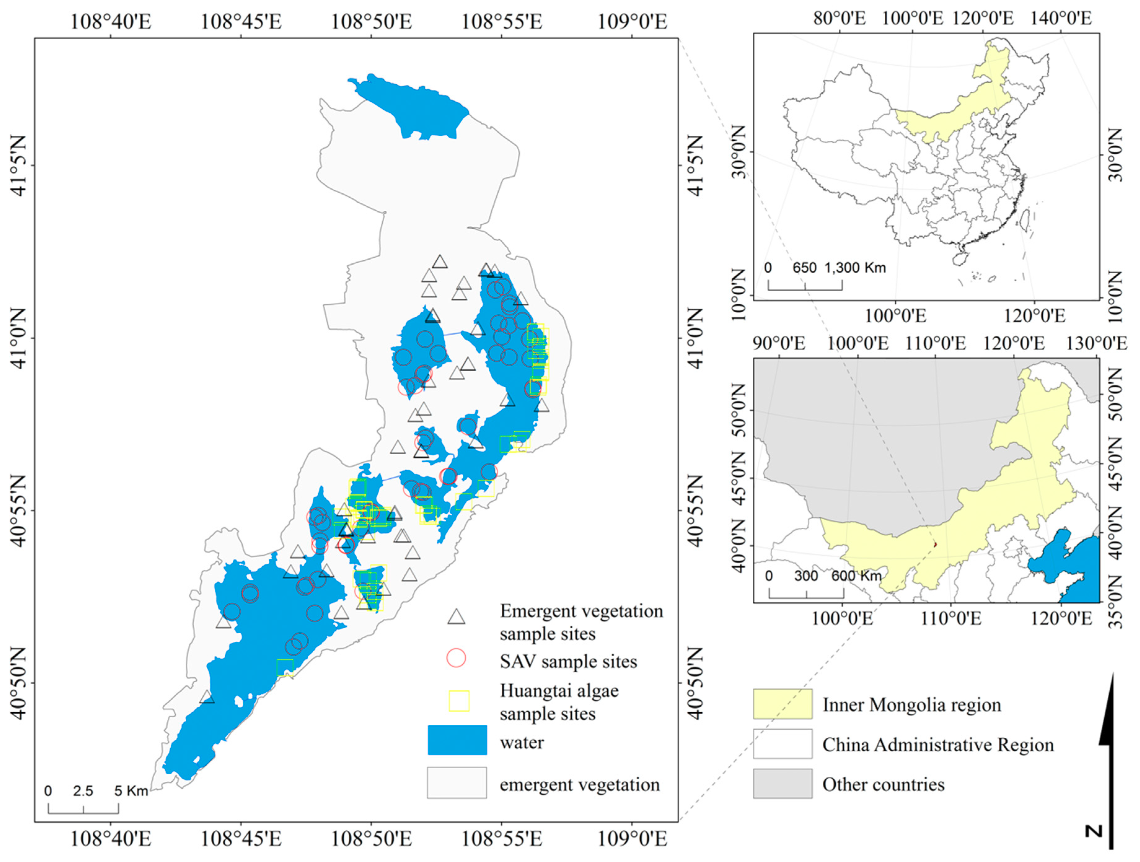
2.1. Study Area

Lake Ulansuhai is the largest freshwater lake in the Yellow River Basin, and the only drainage area in the Hetao irrigation region. Located in Bayannur, Inner Mongolia, Lake Ulansuhai has a longitude from 108°43′–108°57′E and a latitude from 40°36′–41°03′N. The region lies in a temperate continental climate and has alternating seasons with a multiyear average precipitation of 221.1 mm and a multiyear average evaporation of 2382.1 mm. The lake depth ranges from 0.5–2.5 m, and the storage capacity of the lake is 0.32 billion m3. Lake Ulansuhai is classified as a severely eutrophic weed-type lake [32]. The aquatic vegetation in Lake Ulansuhai could be generally classified as emergent vegetation, SAV, and Huangtai algae. Huangtai algae are composed of multiple filamentous algae of chlorophytes Zygophyceae, Zygnematales, and Zygnemataceae, and mainly contain Spirogyra, Zygnema, and Mongeotia algae [33]. Dominant species of aquatic vegetation in Lake Ulansuhai are shown in Figure 1.

2.2. Remote Sensing Data and Processing

The GF-1 satellite carries a 2-m panchromatic camera, an 8-m multispectral camera, and four 16-m wide field view (WFV) cameras, and was launched by China on 26 April 2013. To classify aquatic vegetation, GF-1 WFV images with a resolution of 16 m were chosen, including three visible light bands (blue (band 1), green (band 2), and red (band 3)), and one NIR band (band 4), which are similar to the first four bands of Landsat TM images. With the four multispectral cameras combined, a swath width of 800 km was achieved. The specifications of GF-1 WFV cameras are shown in Table 1. Two images that showed abundant vegetation information from Lake Ulansuhai on 2 July and 8 August in 2015 were selected as the classification data source (because the image on 8 August 2015 contained some cloud, the cloudy part was removed). The Environment for Visualizing Images (ENVI) was used for image pre-processing of ortho-rectification, radiometric calibration, and atmospheric correction. The Fast Line-of-sight Atmospheric Analysis of Spectral Hypercubes (FLAASH) algorithm was adopted for atmospheric correction. The FLAASH model has been used as an effective method for the atmospheric correction of GF-1 images, and can provide accurate surface reflectance [34,35]. Landsat8 Operational Land Imager (OLI) data was used as the reference image for geometric correction, with correction error controlled within 0.5 pixels. The GF-1 data were provided by the China Centre for Resources Satellite Data and Application.

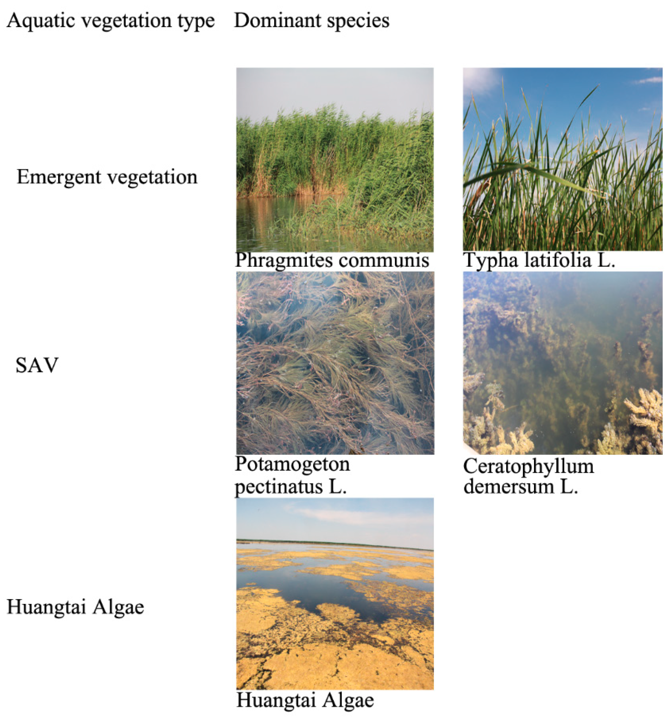
2.3. Acquisition of Field Data

Approximately at the acquisition time of the GF-1 images, a simultaneous field investigation was carried out from 2–5 July and 8–10 August 2015, totaling 146 investigation points, as shown in Figure 2. In July and August 2015, the numbers of emergent vegetation sample points were 23 and 21, the numbers of SAV sample points were 32 and 25, and the numbers of Huangtai algae sample points were 25 and 20, respectively. The sampling locations were set according to the aquatic vegetation distribution, and were chosen such that the investigation covered the whole lake. The location coordinates and type of vegetation at each point were recorded. The sample area for all investigation points was over 64 m × 64 m (or equivalent to four pixels of GF-1 data). To further explore the spectral curve characteristics of SAV and water, the reflectance of SAV and water were measured with an Analytica Spectra Devices, Inc. (ASD) FieldSpec® Handheld2™ Spectroradiometer in July 2016. The spectral curve changes of SAV with depth under different conditions were also measured in June 2018 unsing ASD FieldSpec® 4 spectroradiometer. The wavelength response range of FieldSpec® Handheld2™ and FieldSpec® 4 spectroradiometer is 325–1075 nm and 350–2500 nm, respectively. Because of the presence of noise in the signal, we used only the range 350–900 nm.

2.4. Methods

The aquatic vegetation in Lake Ulansuhai was divided into three types, based on field monitoring: emergent vegetation, SAV, and Huangtai algae. Because of the flowering of vegetation in August, WFV1 image from GF-1 on 8 August 2015 was selected to analyze the spectral characteristics of different classes. ENVI 5.1 was used to plot the average spectral signature for different classes by combining endmember sample points at different locations for each class.

2.4.1. Identification and Detection of Land and Emergent Vegetation

According to Figure 3, the land had a very high reflectance in the third band, meaning that band 3 could be used to identify land. Because of the chlorophyll content of emergent vegetation, it had strong absorption in blue and red light. Therefore, absorption valleys appeared in bands 1 and 3. As the emergent vegetation absorbed less green light, a small reflectance peak appeared in the green band. In the NIR band, the different refractive indices of the cell wall and lacuna inside the leaf caused multiple reflections, forming a high-reflection region [36]. The reflectance of emergent vegetation in band 4 was higher than the reflectance of other vegetation, and because the reflectance difference in bands 2 and 3 was also relatively high, band 4 or the combination of bands 2 and 3 could be used to extract the presence of emergent vegetation.

2.4.2. Identification and Detection of Huangtai Algae

Figure 3 shows that the spectral curve of Huangtai algae showed a high reflectance typical of vegetation in NIR. Therefore, NDVI could be used to distinguish Huangtai algae from the water body. The spectral curve of Huangtai algae with low density was observed to be similar to that of SAV. Huangtai algae has a yellowish color, which leads to increased reflectance in the red-light band (band 3) [33]. Huangtai algae had a relatively high reflectance in both bands 2 and 3, but SAV did not show a high reflectance in band 3 due to absorption at this wavelength, meaning that Huangtai algae and SAV could be distinguished from each other using B3–B2, calculated from their difference in bands 2 and 3.

2.4.3. Identification and Detection of Water and SAV

The reflectance of water and SAV fluctuates within a certain range around the average spectral curve. Because of the effects of water, the reflectance in the NIR and the red-light bands of aquatic vegetation growing underwater is weakened [37]. A rapid decrease in reflectance in the NIR band was observed as the aquatic vegetation was covered by water, but the absorption of red light was less. When SAV growth reached 43–51 cm below clear water, Cho et al. measured that the NDVI value was close to zero using multiple sensors because the NIR reflectance was completely weakened to the value of red-light reflectance [38].
Figure 4a,b show the field-measured submerged vegetation and water spectral curves. The macrophytes above the water surface showed typical spectral characteristics of green vegetation, with reflection valleys at approximately 675 nm, a sharp reflectance increase at approximately 700 nm, and strong reflection in the NIR band (770–890 nm). The water also showed a reflection peak near 700 nm, after which the reflectance decreased because of the strong absorption of the water body, resulting in a low reflectance in the NIR band. Therefore, it was easy to divide the macrophytes above the water surface from the water body by judging whether there was a high reflectance in the NIR band. However, because of the impact of the water body, the reflectance of macrophytes below the water surface in the NIR band was greatly reduced and did not show a high reflectance, making them difficult to distinguish from the water body.
Based on the spectral response function of WFV1, the convolution method was applied to the ASD spectral field data to calculate the equivalent surface reflectance of submerged vegetation and water in four bands. We simulated GF-1 satellite data to further analyze the spectral characteristics of submerged vegetation and water. The equation is as follows:
< R i > = λ 1 λ 2 S i ( λ ) R ( λ ) d λ λ 1 λ 2 S i ( λ ) d λ  
where R i denotes the equivalent surface reflectance of the ith band of WFV1, λ 1 to λ 2 is the spectral wavelength range of the ith band of WFV1, R ( λ ) is the corresponding reflectance at wavelength λ , and S i ( λ ) is the corresponding response value of the spectral response function of the ith band of WFV1 at wavelength λ .
The equivalent reflectance of submerged vegetation and the water body are shown in Figure 5a–c. The macrophytes above the water surface showed high reflectance in the NIR band and could be easily distinguished from the water body (Figure 5a). Figure 5b shows that some macrophytes growing below the water surface did not show high reflectance in the NIR band, and the reflectance of band 4 was lower than the reflectance of band 3, making its spectral characteristic curves similar to the spectral characteristic curves of water, increasing the difficulty of identifying the macrophytes using NDVI. The water spectral curve inflection point of band 3 remained convex, while the SAV curve still had an absorption valley in band 3 with the curve around this inflection point either concave or convex with small convexity, which is consistent with the experimental results obtained by Cho et al. [39]. To distinguish between SAV and water, a concave–convex decision function was constructed, expressed as follows:
F = ( B 4 B 3 ) / 0.114 ( B 3 B 2 ) / 0.12
in which F denotes the concave–convex decision function. The value 0.114 denotes the difference between the central wavelength of band 4 and band 3; 0.12 denotes the difference between the central wavelength of band 3 and band 2. (B4 − B3)/0.114 denotes the slope of the spectral curve between bands 3 and 4, k1; and (B3 − B2)/0.12 denotes the slope of the spectral curve between bands 2 and 3, k2.
Equation (2) denotes k1 − k2. When the curve around the inflection point is concave, (k1 − k2) > 0. When the curve around the inflection point is convex, (k1 − k2) < 0. Thus, a concave shape yields positive values, while a convex shape yields negative values.
Spectral characteristic curves of water and aquatic vegetation covered by water on GF-1 WFV images are shown in Figure 6. In this figure, the spectral curve of water had a convex shape at the inflection point of band 3, and the spectral curve of SAV had a concave shape at the inflection point of band 3. If we assume the spectral characteristic curve functions of water and SAV are A(X) and B(X), respectively, k1, k2, k1 − k2, |k1 − k2|, and obtuse angle (α) at the inflection point can be calculated as shown in Table 2. Table 2 shows that k1 − k2 of the spectral curve of water was negative, while k1 − k2 of the SAV spectral curve was positive. As the relative concavity or convexity of the spectral curve at the inflection point in band 3 increased, the obtuse angle decreased, and |k1 − k2| increased. In this case, |k1 − k2| is an appropriate metric to quantify the concavity and convexity of the different spectra.
Changes in transparency, depth, and coverage of SAV affect the reflectance of SAV. In order to further explore the transferability of the concave–convex decision function, we studied the effect of transparency, SAV depth, and coverage on the spectral curves of SAV. We conducted experiments with two different transparencies (0.6 m and 1.5 m), and we also set experiments on SAV with different coverage. SAV coverage ranged from 40% to 100%, and the SAV depth below the water surface ranged from 0 m to 1.3 m. The reflectance spectra of SAV was integrated to the four spectral bands of GF-1 using Equation (1).

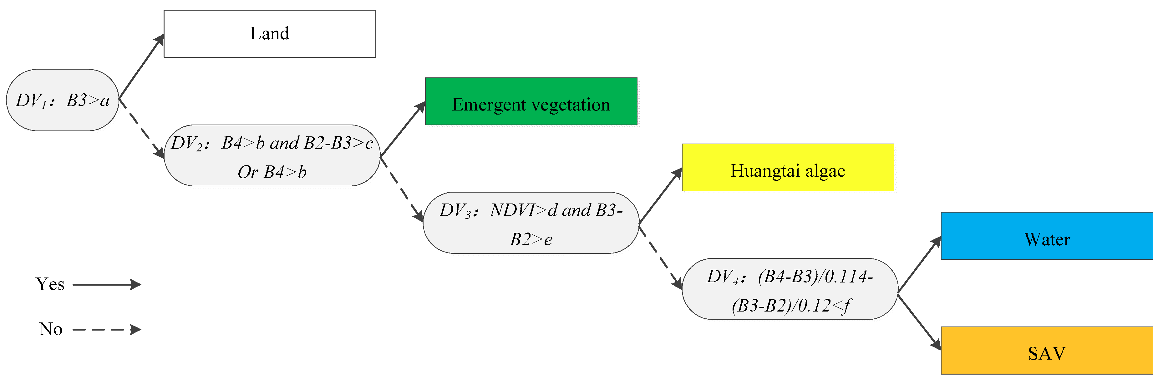
2.4.4. Establishment of the Classification Tree Model

We propose decision variables based on the above analysis, namely, the concave–convex decision function, the single band, and combinations of multiple-bands. These were incorporated in the construction of a decision tree model for aquatic vegetation classification, as shown in Figure 7, where DV denotes decision variable, and a, b, c, d, e, and f denote the optimum threshold values of the decision variables.
Threshold values in the decision tree were repeatedly adjusted and modified according to 50% of the field survey sample points to obtain the optimum threshold values (the other 50% of field sample points were used for validation).

3. Results

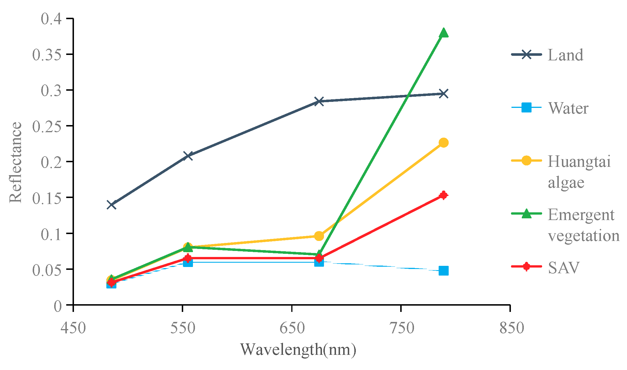
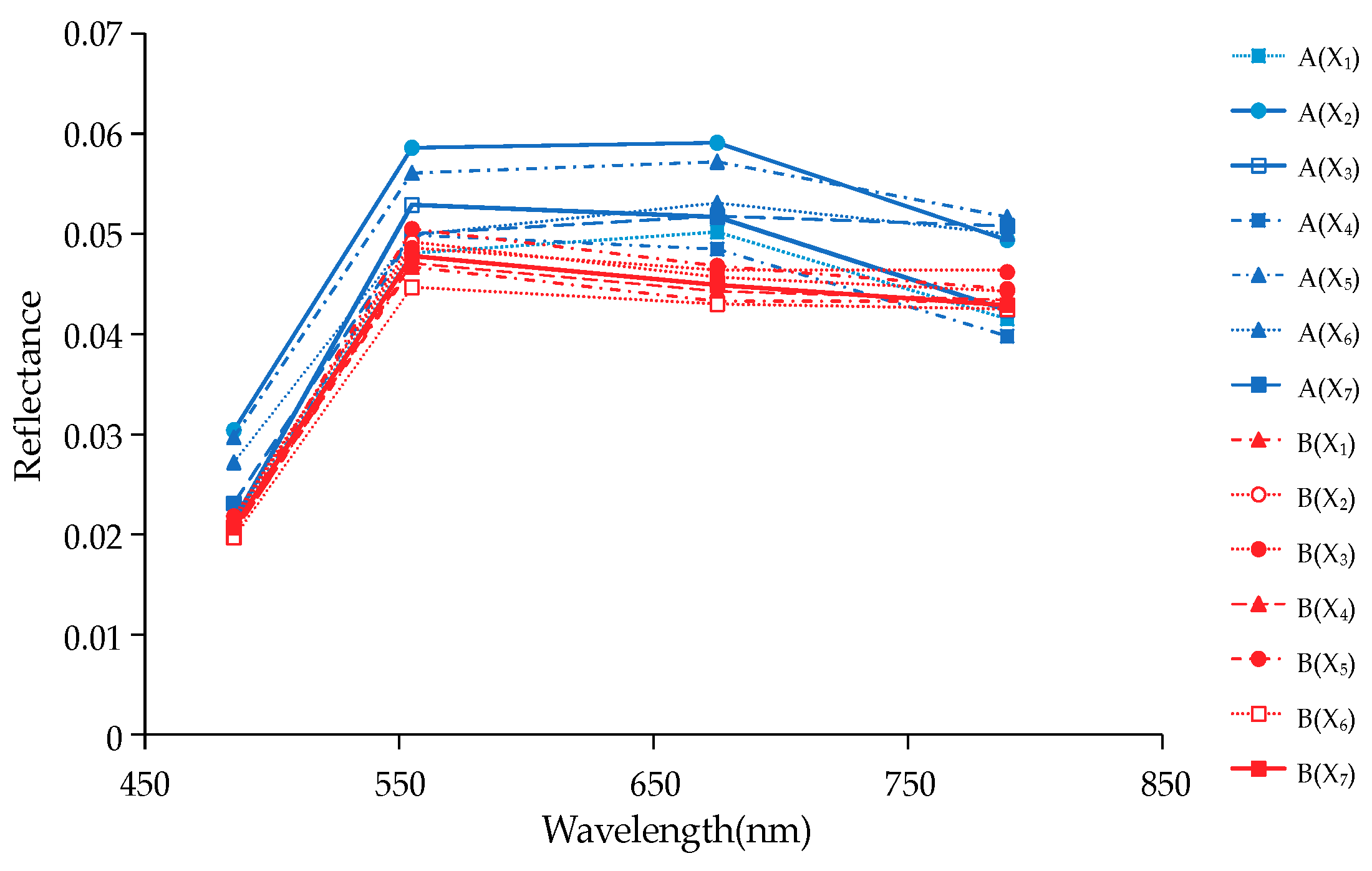
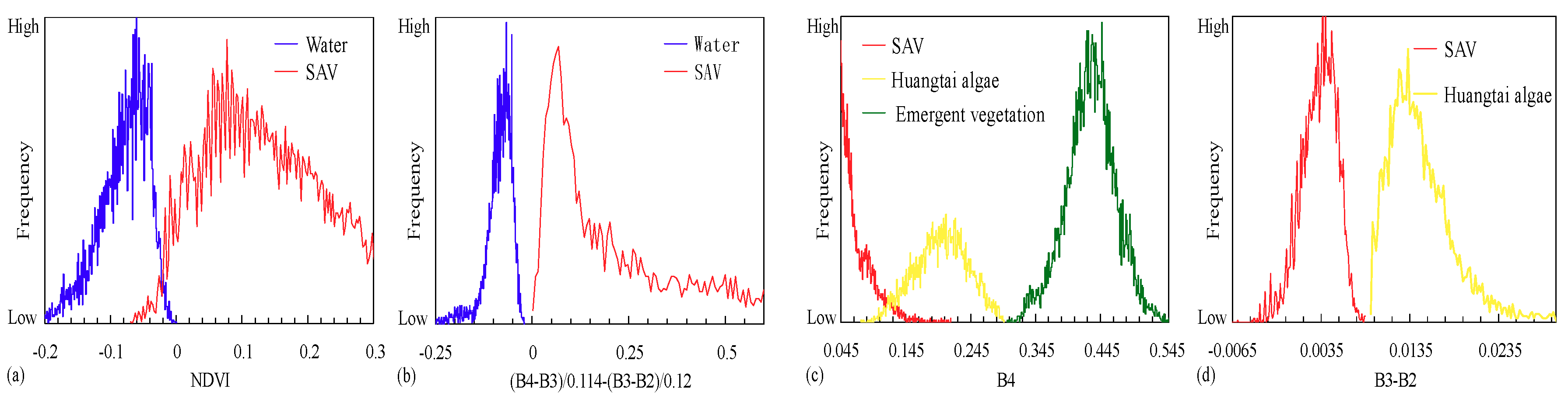
3.1. Separability of Spectral Characteristic Variables

NDVI can generally differentiate between water and vegetation, but it is unable to efficiently extract aquatic vegetation underwater because of the interference from the body of water. The image of Lake Ulansuhai in August of 2015 was used to calculate the frequency distribution of different objects in the areas of interest. Figure 8a shows that water and SAV had a large overlapping area when classified using NDVI, which led to a decrease in classification accuracy as water and SAV were confused. However, when classified using the concave–convex decision function, water and SAV could be distinguished well (Figure 8b), indicating that the concave–convex decision function was better than NDVI in the accurate classification of water and SAV. Figure 8c shows that emergent vegetation was distinguishable from other vegetation using band B4. Huangtai algae and SAV could be differentiated using a combination of bands B3 and B2 (Figure 8d).

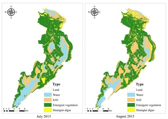
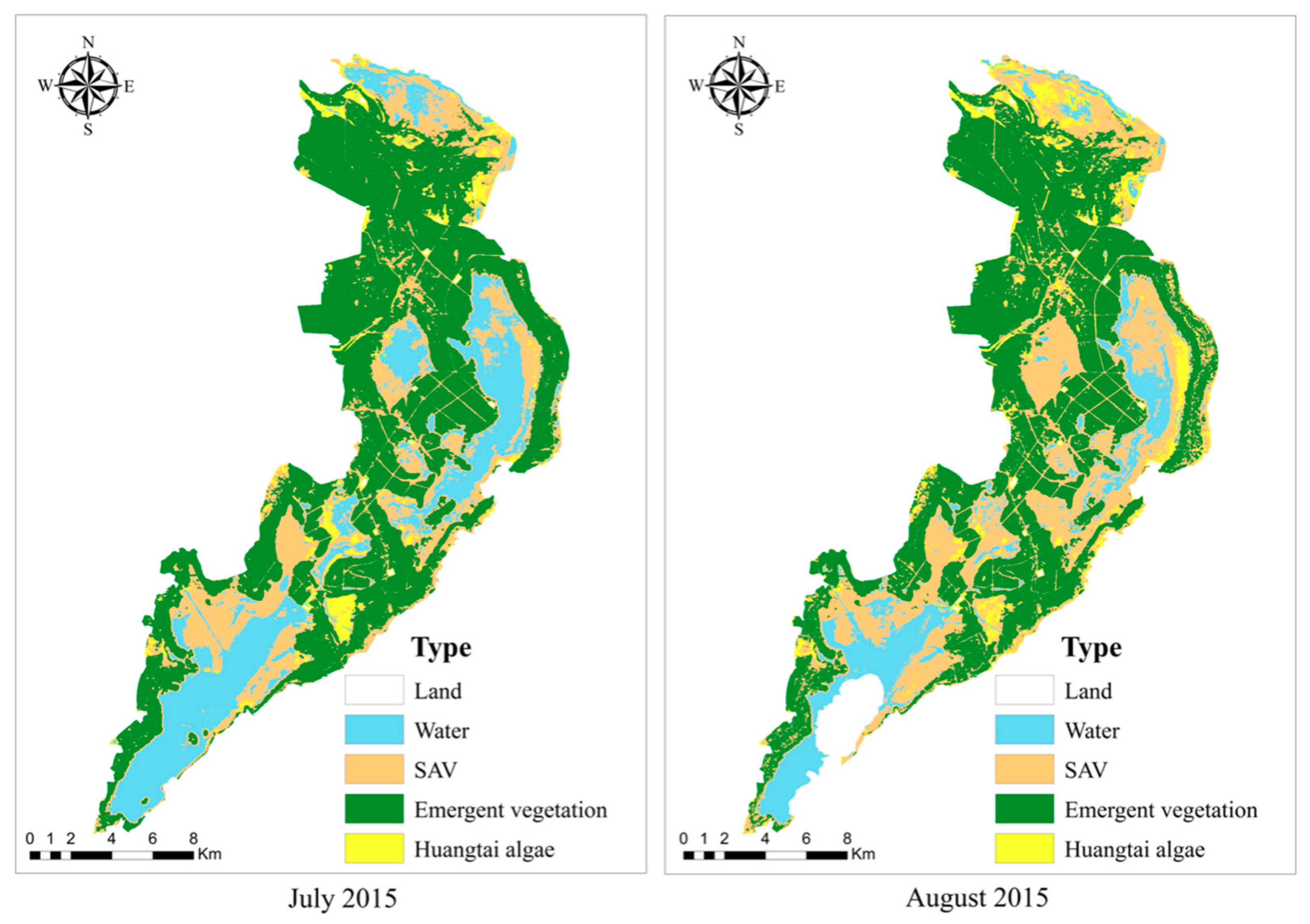
3.2. Classification Results and Validation

Information about aquatic vegetation was extracted from satellite images in July and August of 2015 using the aquatic vegetation classification tree model. The spatial distribution of all vegetation types was obtained as shown in Figure 9.
The confusion matrix and kappa coefficient [40,41] are commonly used methods for the evaluation of the accuracy of vegetation classification. Each column in the confusion matrix represents the ground-truthed classification of one class, and each value in the column is equal to the number of real pixels of the ground surface that were classified in different categories in the classification graph [42].
The confusion matrix based on 50% of the sample data from both the July and August 2015 image classification is shown in Table 3, showing that the overall accuracy of the two classifications was 92.17% and 91.79%, respectively, and the kappa coefficients were 0.8995 and 0.8935, respectively. These results indicate a relatively good classification performance, which provides a theoretical basis for dynamic monitoring of aquatic vegetation in Lake Ulansuhai.
The producer and user accuracies of SAV in August 2015 were 93.85% and 91.04%, respectively. The producer and user accuracies of Huangtai algae were 93.33% and 84.00%, respectively. NDVI was also used to distinguish between water and SAV, resulting in SAV producer and user accuracies of 69.23% and 84.91%, respectively, and in SAV test samples, 26.15% of SAV was classified as water. Clearly, the method proposed in this study greatly improved the classification accuracy.

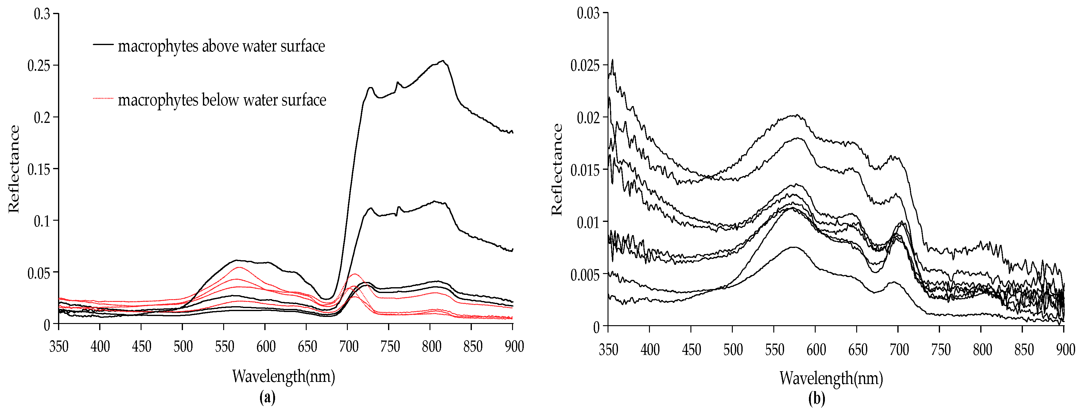
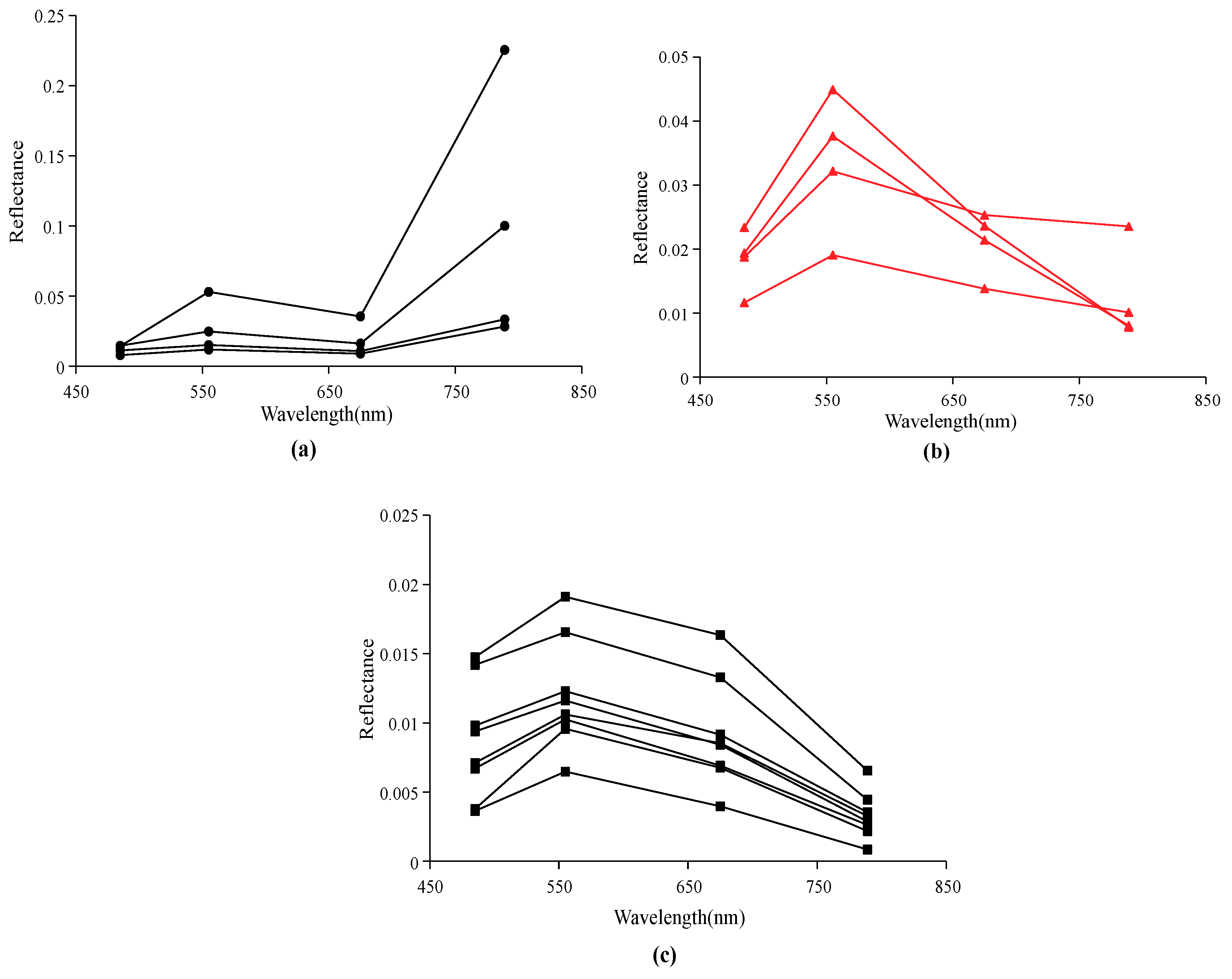
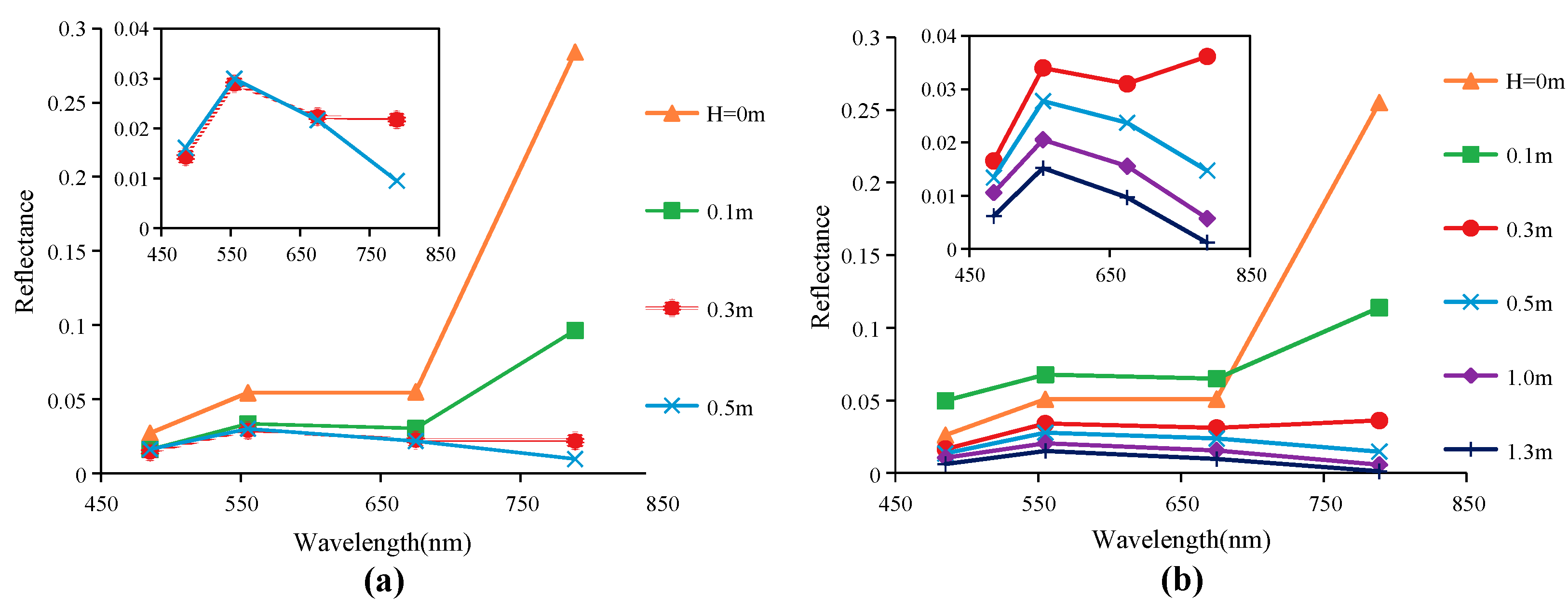
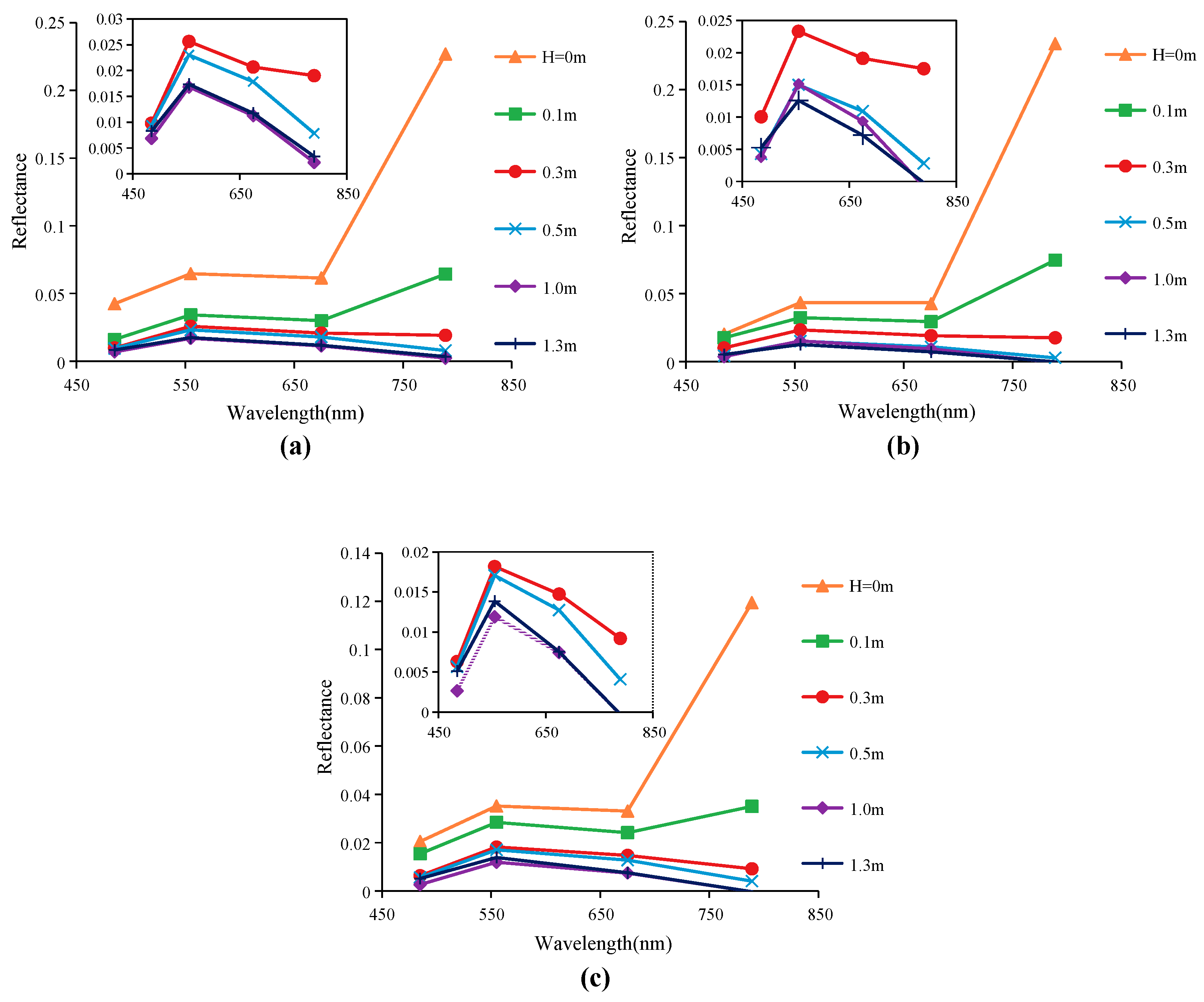
3.3. SAV Spectral Curve Changes with Depth under Different Transparency and Coverage

Figure 10 shows the variation of the SAV reflectance with depth below the water surface under different transparencies in the four bands of GF-1. The vegetation coverage was 100% and the water depth varied from 0 m to 0.5 m and 1.3 m. The NIR reflectance continuously decreased with increasing water depth. With 0.6 m transparency, the typical NIR high reflectance in the vegetation spectra was preserved up to 0.1 m, but was not visible for depths greater than 0.3 m. In a water body with a transparency of 1.5 m, the NIR reflectance decreased by 85.82% from 0 m to 0.3 m, but the NIR reflectance was still higher than that in the red band.
Figure 11 shows the effects of vegetation coverage and depth on the SAV reflectance. When the SAV coverage was 80% and 60%, the NIR high peak could be detected above 0.1 m, and was not visible at 0.3 m. The NIR reflectance of SAV with 80% and 60% coverage decreased by 91.61% and 92.51% from 0 m to 0.3 m, respectively. When SAV coverage was 40%, the NIR reflectance of SAV from 0 m to 0.3 m decreased by 92.29%, and the NIR did not show high reflection characteristics.

4. Discussion

In this study, a decision tree classification was developed for classifying GF-1 imagery to extract the aquatic vegetation in Lake Ulansuhai. The use of this decision tree achieved high classification accuracy in two GF-1 images. However, there are still certain limitations to the application of this method. Huangtai algae started growing in May, and it was difficult to detect it at this time. In addition, SAV turned yellow after September, and its reflectance no longer showed any significant difference from the Huangtai algae in band 3. Therefore, this decision tree method is only applicable to the flowering season of aquatic vegetation in summer. Changes in the weather condition also affected the classification results, and thus the method is applicable to clear and cloudless weather (as applies to most satellite surveys). Most confusion of this method occurred in the extraction of land. This was due to the existence of mixed pixels, and some land edges of islands in the lake were classified as Huangtai algae. In the verification of the classification results, the producer accuracy of land in July and August was 82.61% and 75%, respectively. The water bodies achieved high classification accuracy in July and August, and their producer accuracy was 93.94% and 94.29%, respectively. However, a small part of the water was still classified as SAV because, in some channels, water had similar spectral characteristics to that of nearby vegetation due to limits in image resolution, indicating that it might be difficult to accurately extract channel water for remote sensing products at this resolution. In July, only 2.17% of SAV was classified as water, which was mainly due to the mixed pixels of SAV and water. Only 1.54% of the SAV was classified as water in August, which was mainly caused by low vegetation coverage and water transparency. The error of the emergent vegetation was mainly present in its incorrect division into SAV, which was largely due to the sparseness of the reeds in some areas and mixed pixels with the water and SAV. Huangtai algae achieved high producer accuracy of 92.86% and 93.33% in July and August, respectively. In July, 3.57% of Huangtai algae was mistakenly classified as SAV. A total of 2.22% of Huangtai algae was misclassified as SAV in August. This may have been caused by the sparseness of Huangtai algae and mixture in the same pixel with SAV.
This study demonstrates that there is a sufficient difference in the spectral concavity and convexity between macrophytes below the water surface and water, and the concave–convex decision function could efficiently identify and detect the aquatic vegetation below the water surface. The spectral reflectance curves of submerged vegetation areas and non-submerged vegetation areas also exhibited similar concave–convex characteristics in Lake Pontchartrain [39]. However, the spectral signal of SAV is affected by various factors, such as water turbidity/transparency, the distance between vegetation canopies and the water surface, and SAV coverage. Liew et al. proved that the spectral curve of SAV can change with the change in water turbidity and water depth [43]. They found that the typical NIR peak of vegetation spectra could not be detected at a water depth of 1 m with turbidity 0.5 NTU, and vegetation could not be detected at 0.5 m with high turbidity (50 NTU). Beget et al. found that the reflectance in NIR of the flooded vegetation decreased as its flooding level increased [21]. Variation in these factors might lead to the change of suitable ranges of the decision function. In order to explore the applicable conditions of the concave–convex decision function under different transparency, vegetation depth, and coverage, we integrated field hyperspectral data to four bands of GF-1 based on Equation (1). This convolution method was based on the band range of GF-1, and the NIR ranged from 0.77–0.89 µm. Various remote sensing sensors may have slightly different calculation results because of their different band ranges. Therefore, the applicability of this method to other sensors still needs further exploration.
As shown in Figure 10, at 0.3 m with 0.6 m transparency, although the NIR peak disappeared, the spectral curve of SAV was still concave in the third band. Thus, SAV could be judged by using the concave–convex decision function in this situation. However, this concave characteristic disappeared at 0.5 m. Overall, in a water body with a transparency of 0.6 m, the concave–convex decision function could be applied to 100% SAV coverage above 0.3 m. Below 0.3 m, both the water body and the SAV showed a convex shape in the third band, and they could be determined based on the included angle of the concave–convex decision function. In a 1.5-m transparency water body, the vegetation NIR peak still existed at 0.3 m due to SAV coverage of 100% and the high transparency of the water body, but it disappeared at 0.5 m. The range in which the SAV spectral curve was concave in the third band should be between 0.3 m and 0.5 m, but we did not capture the specific value because of the large interval setting of depth. As described in the results, SAV with 80% and 60% coverage in Figure 11 did not exhibit NIR high peak characteristics at 0.3 m. However, the SAV spectral curve was still concave in the third band at this depth. SAV could also be judged by using the concave–convex decision function. The concave shape of the SAV spectral curves in the third band both disappeared at 0.5 m. With 40% SAV coverage, NIR showed high reflectance above 0.1 m, but at 0.3 m, the concave shape of the SAV spectral curve in the third band disappeared. Therefore, when SAV coverage was less than 40%, even at 0.3 m, it is difficult to identify the SAV based only on the concave shape of the spectral curve. Overall, the concave–convex decision function could be applied to 80% and 60% SAV coverage above 0.3 m and 40% SAV coverage above 0.1 m under 1.5 m transparency.

5. Conclusions

It is almost impossible to accurately identify plants that grow underwater using conventional extraction methods for aquatic vegetation. The concave–convex decision function method proposed in this study could further accurately classify SAV from water bodies. When comparing the results of the concave–convex decision function method with the NDVI classification using the same data, the concave–convex decision function method clearly outperformed the NDVI classification. The decision function can be applied to waters with SAV coverage greater than 40% above 0.3 m and SAV coverage 40% above 0.1 m under 1.5 m transparency. With 100% SAV coverage under 0.6 m transparency, the concave–convex decision function can be applied up to 0.3 m. Combining the concave–convex decision function flexibly in the classification method (e.g., using a decision tree) can achieve the accurate extraction of SAV, and provides new ideas for the accurate extraction of SAV in other regions.
Another outcome of interest from this research is the potential utility of the GF-1 in aquatic vegetation classification. When aquatic vegetation information from two-period GF-1 remote sensing images in July and August 2015 was classified using the decision tree method from Lake Ulansuhai, China, the overall accuracy was 92.17% and 91.79%, respectively. Four bands from GF-1 (a satellite with higher resolution than TM and HJ-1A/B, a shorter revisit period, and good continuity) had relatively good applicability for information extraction of aquatic vegetation. High-resolution GF-1 images combined with a new decision function were able to provide a simple and effective method to dynamically and accurately monitor aquatic vegetation, especially SAV, on a large regional scale, and could provide support for long-term ecosystem health monitoring.

Author Contributions

Q.C. conceived the idea of this study and wrote the paper. R.Y. and Y.H. directed the study. R.Y. and Q.C. designed the experiments. R.Y., Y.H., Q.C., W.Z., Q.Z., and X.B. carried out the field experiments. R.Y., Y.H., and L.W. revised the paper. R.Y. and Y.H. directed the major revision.

Funding

This research was funded by the National Natural Science Foundation of China (Grant Nos. 51469018, 61461034, 91547110 and 41701281); the National Key Research and Development Program of China (Grant No. 2016YFC0500508); and Ministry of Water Resources Special Funds for Scientific Research Projects of Public Welfare Industry (Grant No. 20150104).

Acknowledgments

We are indebted to two anonymous reviewers for their efforts and constructive comments. These comments and suggestions have greatly improved our work.

Conflicts of Interest

The authors declare no conflict of interest.

References

  1. Jin, X. Lake Environment in China; China Ocean Press: Beijing, China, 1995. [Google Scholar]
  2. Ma, R. Remote Sensing of Lake Water Environment; Science Press: Beijing, China, 2010. [Google Scholar]
  3. Silva, T.S.F.; Costa, M.P.F.; Melack, J.M.; Novo, E.M.L.M. Remote sensing of aquatic vegetation: Theory and applications. Environ. Monit. Assess. 2008, 140, 131–145. [Google Scholar] [CrossRef] [PubMed]
  4. Marshall, T.R.; Lee, P.F. Mapping aquatic macrophytes through digital image analysis of aerial photographs: An assessment. J. Aquat. Plant Manag. 1994, 32, 61–66. [Google Scholar]
  5. Welch, R.; Remillard, M.M.; Slack, R.B. Remote sensing and geographic information system techniques for aquatic resource evaluation. Photogramm. Eng. Remote Sens. 1988, 54, 177–185. [Google Scholar]
  6. Zhang, Y.; Liu, X.; Qin, B.; Shi, K.; Deng, J.; Zhou, Y. Aquatic vegetation in response to increased eutrophication and degraded light climate in eastern lake Taihu: Implications for lake ecological restoration. Sci. Rep. 2016, 6. [Google Scholar] [CrossRef] [PubMed]
  7. Fusilli, L.; Collins, M.O.; Laneve, G.; Palombo, A.; Pignatti, S.; Santini, F. Assessment of the abnormal growth of floating macrophytes in Winam Gulf (Kenya) by using MODIS imagery time series. Int. J. Appl. Earth Obs. Geoinf. 2013, 20, 33–41. [Google Scholar] [CrossRef]
  8. Ackleson, S.G.; Klemas, V. Remote sensing of submerged aquatic vegetation in lower Chesapeake Bay: A comparison of Landsat MSS to TM imagery. Remote Sens. Environ. 1987, 22, 235–248. [Google Scholar] [CrossRef]
  9. Armstrong, R.A. Remote sensing of submerged vegetation canopies for biomass estimation. Int. J. Remote Sens. 1993, 14, 621–627. [Google Scholar] [CrossRef]
  10. Luo, J.; Li, X.; Ma, R.; Li, F.; Duan, H.; Hu, W.; Qin, B.; Huang, W. Applying remote sensing techniques to monitoring seasonal and interannual changes of aquatic vegetation in Taihu Lake, China. Ecol. Indic. 2016, 60, 503–513. [Google Scholar] [CrossRef]
  11. Xie, Y.; Sha, Z.; Yu, M. Remote sensing imagery in vegetation mapping: A review. J. Plant Ecol. 2008, 1, 9–23. [Google Scholar] [CrossRef]
  12. Dogan, O.K.; Akyurek, Z.; Beklioglu, M. Identification and mapping of submerged plants in a shallow lake using quickbird satellite data. J. Environ. Manag. 2009, 90, 2138–2143. [Google Scholar] [CrossRef] [PubMed]
  13. Pu, R.; Bell, S. Mapping seagrass coverage and spatial patterns with high spatial resolution IKONOS imagery. Int. J. Appl. Earth Obs. Geoinf. 2017, 54, 145–158. [Google Scholar] [CrossRef]
  14. Whiteside, T.; Bartolo, R. Mapping aquatic vegetation in a tropical wetland using high spatial resolution multispectral satellite imagery. Remote Sens. 2015, 7, 11664–11694. [Google Scholar] [CrossRef]
  15. Bolpagni, R.; Bresciani, M.; Laini, A.; Pinardi, M.; Matta, E.; Ampe, E.M.; Giardino, C.; Viaroli, P.; Bartoli, M. Remote sensing of phytoplankton-macrophyte coexistence in shallow hypereutrophic fluvial lakes. Hydrobiologia 2014, 737, 67–76. [Google Scholar] [CrossRef]
  16. Wang, Y.; Traber, M.; Milstead, B.; Stevens, S. Terrestrial and submerged aquatic vegetation mapping in fire island national seashore using high spatial resolution remote sensing data. Mar. Geod. 2007, 30, 77–95. [Google Scholar] [CrossRef]
  17. Lin, C.; Gong, Z.; Zhao, W. The extraction of wetland hydrophytes types based on medium resolution TM data. Acta Ecol. Sin. 2010, 30, 6460–6469. [Google Scholar]
  18. Zhao, D.; Lv, M.; Jiang, H.; Cai, Y.; Xu, D.; An, S. Spatio-temporal variability of aquatic vegetation in Taihu Lake over the past 30 years. PLoS ONE 2013, 8, 10454–10461. [Google Scholar] [CrossRef] [PubMed]
  19. Davranche, A.; Lefebvre, G.; Poulin, B. Wetland monitoring using classification trees and spot-5 seasonal time series. Remote Sens. Environ. 2010, 114, 552–562. [Google Scholar] [CrossRef] [Green Version]
  20. Ma, R.; Duan, H.; Gu, X.; Zhang, S. Detecting aquatic vegetation changes in Taihu Lake, China using multi-temporal satellite imagery. Sensors 2008, 8, 3988–4005. [Google Scholar] [CrossRef] [PubMed]
  21. Beget, M.E.; Bella, C.M.D. Flooding: The effect of water depth on the spectral response of grass canopies. J. Hydrol. 2007, 335, 285–294. [Google Scholar] [CrossRef]
  22. Zhang, S.; Duan, H.; Gu, X. Remote sensing information extraction of hydrophytes based on the retrieval of water transparency in lake Taihu, China. J. Lake Sci. 2008, 20, 184–190. [Google Scholar] [CrossRef]
  23. Li, F.; Xiao, B. Aquatic vegetation mapping based on remote sensing imagery: An application to Honghu Lake. In Proceedings of the International Conference on Remote Sensing, Environment and Transportation Engineering, Nanjing, China, 24–26 June 2011; pp. 4832–4836. [Google Scholar]
  24. Visser, F.; Wallis, C.; Sinnott, A.M. Optical remote sensing of submerged aquatic vegetation: Opportunities for shallow clearwater streams. Limnol. Ecol. Manag. Inland Waters 2013, 43, 388–398. [Google Scholar] [CrossRef] [Green Version]
  25. Alberotanza, L. Hyperspectral aerial images. A valuable tool for submerged vegetation recognition in the Orbetello Lagoons, Italy. Int. J. Remote Sens. 1999, 20, 523–533. [Google Scholar] [CrossRef]
  26. Li, J.; Wu, D.; Wu, Y.; Liu, H.; Shen, Q.; Zhang, H. Identification of algae-bloom and aquatic macrophytes in Lake Taihu from in-situ measured spectra data. J. Lake Sci. 2009, 21, 215–222. [Google Scholar] [Green Version]
  27. Cho, H.J.; Lu, D. A water-depth correction algorithm for submerged vegetation spectra. Remote Sens. Lett. 2010, 1, 29–35. [Google Scholar] [CrossRef] [Green Version]
  28. Cho, H.J.; Mishra, D.; Wood, J. Remote sensing of submerged aquatic vegetation. In Remote Sensing—Applications; Escalante, B., Ed.; InTech: Rijeka, Croatia, 2012. [Google Scholar]
  29. Wang, L.; Yang, R.; Tian, Q.; Yang, Y.; Zhou, Y.; Sun, Y.; Mi, X. Comparative analysis of GF-1 WFV, ZY-3 MUX, and HJ-1 CCD sensor data for grassland monitoring applications. Remote Sens. 2015, 7, 2089–2108. [Google Scholar] [CrossRef]
  30. Xia, C.; Zhang, Y.; Wang, W. A relief-based forest cover change extraction using GF-1 images. In Proceedings of the IGARSS 2014—2014 IEEE International Geoscience and Remote Sensing Symposium, Quebec, QC, Canada, 13–18 July 2014. [Google Scholar]
  31. Yang, Y.; Zhan, Y.; Tian, Q.; Gu, X.; Yu, T.; Wang, L. Crop classification based on GF-1/WFV NDVI time series. Trans. Chin. Soc. Agric. Eng. 2015, 31, 155–161. [Google Scholar]
  32. He, L.; Xi, B.; Lei, H. Research on Integrated Treatment and Management Planning of Lake Ulansuhai; China Environmental Science Press: Beijing, China, 2013. [Google Scholar]
  33. Zheng, W.; Han, X.; Liu, C. Satellite remote sensing data monitoring “Huang Tai” algae bloom in lake Ulansuhai, inner Mongolia. J. Lake Sci. 2010, 22, 321–326. [Google Scholar]
  34. Jia, K.; Liang, S.; Gu, X.; Baret, F.; Wei, X.; Wang, X.; Yao, Y.; Yang, L.; Li, Y. Fractional vegetation cover estimation algorithm for chinese GF-1 wide field view data. Remote Sens. Environ. 2016, 177, 184–191. [Google Scholar] [CrossRef]
  35. Wu, Z.; Yang, F.; Zhang, Y.; Wu, Y.; Yu, W. Quality evaluation of GF-1 and SPOT-7 multi-spectral image based on land surface parameter validation. J. Image Graph. 2016, 21, 1551–1561. [Google Scholar]
  36. Zhao, Y. Principles and Methods of Analysis of Remote Sensing Applications; Science Press: Beijing, China, 2003. [Google Scholar]
  37. Han, L.; Rundquist, D.C. The spectral responses of Ceratophyllum demersum at varying depths in an experimental tank. Int. J. Remote Sens. 2003, 24, 859–864. [Google Scholar] [CrossRef]
  38. Cho, H.J.; Kirui, P.; Natarajan, H. Test of multi-spectral vegetation index for floating and canopy-forming submerged vegetation. Int. J. Environ. Res. Public Health 2008, 5, 477. [Google Scholar] [CrossRef] [PubMed]
  39. Cho, H.J. Depth-variant spectral characteristics of submersed aquatic vegetation detected by Landsat 7 ETM+. Int. J. Remote Sens. 2007, 28, 1455–1467. [Google Scholar] [CrossRef]
  40. Cohen, J. A coefficient of agreement for nominal scales. Educ. Psychol. Meas. 1960, 20, 37–46. [Google Scholar] [CrossRef]
  41. Cohen, J. Weighted kappa: Nominal scale agreement with provision for scaled disagreement or partial credit. Psychol. Bull. 1968, 70, 213–220. [Google Scholar] [CrossRef] [PubMed]
  42. Jensen, J.R. Introductory Digital Image Processing a Remote Sensing Perspective; Science Press: Beijing, China, 2007. [Google Scholar]
  43. Liew, S.C.; Chang, C.W. Detecting submerged aquatic vegetation with 8-band worldview-2 satellite images. In Proceedings of the Geoscience and Remote Sensing Symposium, Munich, Germany, 22–27 July 2012; pp. 2560–2562. [Google Scholar]
Figure 1. Dominant species of aquatic vegetation in Lake Ulansuhai. SAV: submerged aquatic vegetation.
Remotesensing 10 01279 g001
Figure 2. Aquatic vegetation samples in Lake Ulansuhai.
Remotesensing 10 01279 g002
Figure 3. Spectral curves of different classes.
Remotesensing 10 01279 g003
Figure 4. The field-measured spectral curves of (a) submerged vegetation and (b) water.
Remotesensing 10 01279 g004
Figure 5. Equivalent surface reflectance of submerged vegetation and water. Equivalent reflectance of macrophytes (a) above and (b) below the water surface, respectively. (c) The equivalent reflectance of water.
Remotesensing 10 01279 g005
Figure 6. Spectral curves of water and macrophytes underwater. Blue curves denote spectral curves of water, and red curves denote spectral curves of SAV. A(X) and B(X) denote the spectral characteristic curve functions of water and SAV, respectively.
Remotesensing 10 01279 g006
Figure 7. Classification tree model of aquatic vegetation. DV denotes a decision variable, and a, b, c, d, e, and f denote the optimum threshold values of the decision variables. NDVI: normalized difference vegetation index.
Remotesensing 10 01279 g007
Figure 8. Statistical frequency distribution of different classes. The statistical frequency distribution of water and SAV using (a) NDVI and the (b) concave–convex decision function extraction method. The statistical frequency distribution of three species of vegetation is shown in (c,d).
Remotesensing 10 01279 g008
Figure 9. Aquatic vegetation classification results of remote sensing images in July and August 2015.
Remotesensing 10 01279 g009
Figure 10. Remote sensing reflectance of SAV with 100% vegetation coverage at varying depth below water surface under different transparencies: (a) transparency = 0.6 m; and (b) transparency = 1.5 m. H represents different SAV depth.
Remotesensing 10 01279 g010
Figure 11. SAV remote sensing reflectance at different depths below the water surface under 1.5 m transparency: (a) SAV coverage = 80%; (b) SAV coverage = 60%; and (c) SAV coverage = 40%.
Remotesensing 10 01279 g011
Table 1. Characterization of Gao Fen 1 (GF-1) wide field view (WFV) cameras.
SensorBandSpectral Range (µm)Band TypeSpatial Resolution (m)Swath Width (km)Revisit Period (days)Orbit Altitude (km)
WFV (1–4)10.45–0.52Blue168004645
20.52–0.59Green
30.63–0.69Red
40.77–0.89NIR
Table 2. Calculated values of the spectral curve function for water and macrophytes underwater.
k1k2k1 − k2|k1 − k2|Obtuse Angle α
A(X1)−0.07630.0175–0.09380.0938174.6333
A(X2)−0.08510.0042−0.08930.0893174.8978
A(X3)−0.0816−0.0100−0.07160.0716175.9091
A(X4)−0.0763−0.0117−0.06460.0646176.3043
A(X5)−0.04820.0092−0.05740.0574176.7127
A(X6)−0.02720.0267−0.05390.0539176.9148
A(X7)−0.00880.0150−0.02380.0238178.6380
B(X1)−0.0018−0.02830.02660.0266178.4776
B(X2)−0.0123−0.02920.01690.0169179.0329
B(X3)−0.0018−0.01830.01660.0166179.0502
B(X4)−0.0079−0.02330.01540.0154179.1157
B(X5)−0.0202−0.03080.01070.0107179.3898
B(X6)−0.0044−0.01420.00980.0098179.4397
B(X7)−0.0175−0.02420.00660.0066179.6207
Table 3. Classification accuracy test. SAV: submerged aquatic vegetation.
Real Value
Classification Value LandWaterSAVEmergent VegetationHuangtai AlgaeTotal
Month070807080708070807080708
Land1915000000102015
Water2031331100003434
SAV0022436143215167
Emergent Vegetation0000005539125641
Huangtai2500230052425650
Total23203335466559425645217207
Producer Accuracy (%)82.61 75.00 93.94 94.29 93.48 93.85 93.22 92.86 92.86 93.33
User Accuracy (%)95.00 100.00 91.18 97.06 84.31 91.04 98.21 95.12 92.86 84.00
Kappa Coefficient0.8995 0.8935
Overall accuracy92.17% 91.79%

