SLALOM: An All-Surface Snow Water Path Retrieval Algorithm for the GPM Microwave Imager

Abstract

This paper describes a new algorithm that is able to detect snowfall and retrieve the associated snow water path (SWP), for any surface type, using the Global Precipitation Measurement (GPM) Microwave Imager (GMI). The algorithm is tuned and evaluated against coincident observations of the Cloud Profiling Radar (CPR) onboard CloudSat. It is composed of three modules for (i) snowfall detection, (ii) supercooled droplet detection and (iii) SWP retrieval. This algorithm takes into account environmental conditions to retrieve SWP and does not rely on any surface classification scheme. The snowfall detection module is able to detect 83% of snowfall events including light SWP (down to 1 × 10⁻³ kg·m⁻²) with a false alarm ratio of 0.12. The supercooled detection module detects 97% of events, with a false alarm ratio of 0.05. The SWP estimates show a relative bias of −11%, a correlation of 0.84 and a root mean square error of 0.04 kg·m⁻². Several applications of the algorithm are highlighted: Three case studies of snowfall events are investigated, and a 2-year high resolution 70°S–70°N snowfall occurrence distribution is presented. These results illustrate the high potential of this algorithm for snowfall detection and SWP retrieval using GMI.

1. Introduction

Snowfall plays a central role in the Earth’s climate system. Indeed, it is directly connected to the occurrence of snow on the ground, which itself impacts the climate. First, the surface snow layer strongly affects the water cycle at high latitudes and in mountainous regions by storing water during the cold season and then releasing it progressively in the environment when the weather gets warmer. Secondly, snow covered areas impact the Earth’s radiative budget. Indeed, snow covered surfaces have a much higher albedo than bare land and thus reflect a significant portion of incoming sun radiation, which limits the surface warming. Climate change could alter the spatial and temporal distribution of global snowfall patterns and snow cover. Even a slight increase in temperature can, in some cases, change the precipitation phase from snow to rain. In fact, several studies in the USA already reported a decrease of the proportion of snow events versus rain events in winter time [1,2]. This problem illustrates the strong need to better characterize snow distribution and variability at the global scale.

Global snowfall can only be monitored observationally using spaceborne instruments [3,4]. Spaceborne microwave sensors are particularly suitable for detecting and quantifying snowfall thanks to their unique ability to probe within clouds [5,6]. Active microwave sensors, such as the Cloud Profiling Radar (CPR) onboard CloudSat [7] and the Dual-Frequency Precipitation Radar (DPR) onboard the Global Precipitation Measurement Mission-Core Observatory (GPM-CO, [8]), are particularly valuable for providing detailed vertical profiles of snow [9,10,11,12,13]. However, due to several limitations, such as their reduced swath (especially for CPR) or their limited sensitivity (for DPR), they are not well-suited to comprehensively characterizing snowfall. Specifically, the CPR swath width of 1.7 km implies a revisit time of about two weeks for a 100 km × 100 km pixel. In addition, CPR does not provide snowfall observations close to the surface (i.e., below ~1 km) due to ground clutter, which remains a substantial limitation for quantifying surface snowfall. Regarding DPR, Casella et al. [14] showed that this radar detects only 5–7% of global snowfall events with respect to CPR, while 29–34% of the CPR global snowfall mass is detected by DPR (for version 4 products). They also showed that, while DPR is mostly suitable for retrieving intense/deeper snowfall, and by optimally combining the dual-frequency signal (Ku and Ka band), DPR snowfall detection efficacy can increase significantly (up to 54–59% of the CPR snowfall mass), it misses a significant part of light snowfall events.

On the other hand, passive microwave sensors, such as the most recent GPM Microwave Imager (GMI) or the Advanced Technology Microwave Sounder (ATMS) (on board Suomi-NPP and NOAA-20 satellites), appear promising for snowfall characterization. These sensors have high frequency channels that are highly sensitive to snowfall due to the scattering by snowflakes of upwelling terrestrial and radiation, originating in the lower levels of the atmosphere [15,16,17,18]. In addition, passive microwave radiometers have a large swath and have been installed on many platforms over the last decades, ensuring a good global coverage with a fair spatial resolution and lengthy data records.

Therefore, several approaches have been proposed in recent years for detecting and retrieving snowfall using passive microwave radiometers, such as the Special Sensor Microwave-Humidity (SSM/T2) [19], Advanced Microwave Sounding Unit-B (AMSU-B) and Microwave Humidity Sounding (MHS) [5,16,20,21,22], Advanced Technology Microwave Sounder (ATMS) [23,24], Special Sensor Microwave-Imager/Sounder (SSMIS) [25] and GMI [26] (Figure 1). In addition, to these passive microwave products, specifically dedicated to snowfall, some operational products provide estimations of precipitation, including snowfall at the global scale, combining observations of several radiometers. In particular, the official NASA Goddard PROFiling (GPROF) Bayesian algorithm [27] retrieves precipitation for all the radiometers of the GPM constellation. GPROF is tuned using an a priori database of matching TBs and observed precipitation rates. These observed precipitation rates originate in DPR over vegetated lands and oceans, as well as in the Multi-Radar/Multi-Sensor (MRMS) U.S. ground radar network over snow covered surfaces. The phase classification of the precipitation (solid or liquid) is based on the parameterization scheme of Sims and Liu [28]. GPROF, as well as any algorithm based on the use of empirical datasets, suffers from the limitations of the products used as references. For example, GPROF snowfall retrievals are affected by the low sensitivity of DPR to snowfall (as shown in Casella et al. [14]), and by the difficulties of MRMS in retrieving surface snowfall and representing snowfall events at the global scale.

Despite these attempts, detecting and quantifying surface snowfall rates using spaceborne microwave radiometers remains a challenging task [3,26,29]. The high-frequency radiometer channel observations are very sensitive to environmental conditions (e.g., humidity, temperature, frozen or snow-covered soils), which affect the measured signal. This problem is particularly acute at high latitudes, where the low and variable emissivity of snow or ice-covered surfaces [22,30,31,32] can mask snowflakes’ scattering signatures [33]. Moreover, low humidity in high latitude regions makes the atmosphere more transparent for channels that probe around the water vapor absorption line and thus increase surface contamination. The snow microphysics is also very complex, and a snow cloud is often composed of a gamut of snow particles with a variety of densities, shapes, particle size distributions and radiative properties [34,35,36,37,38,39]. In addition, supercooled droplets and melting snow frequently occur and can strongly affect the observed signal [16,40,41,42]. Finally, while the active sensors, such as CPR, provide vertical information on snow clouds, passive instruments only offer integrated information that combines the radiative signal of every cloud layer.

Recently, Panegrossi et al. [43] highlighted the impact of falling snow on the high frequency GMI channels using CloudSat CPR as a reference. This study focuses on higher latitude snowfall systems (around 60°N/S) and includes very weak snowfall events that are not considered in studies where DPR is used as a reference [26,33]. In particular, Panegrossi et al. [43] identified the environmental conditions under which snow detection could be optimally achieved (e.g., high atmospheric moisture and sea ice coverage) and characterized the sensitivity of GMI high-frequency channels and the polarization signal at 166 GHz to falling snow. They also highlighted the impact of supercooled droplets on the GMI signal, showing that a supercooled droplet layer on top of a snow cloud can filter out the scattering signal of the snow particles below. This study, as well as that of You et al. [26] and Ebtehaj et al. [33], have evidenced the need to characterize the extremely variable background surface for each GMI pixel at the time of the overpass, especially at high latitudes (in cold and dry conditions), where high-frequency channels may be affected by the emission and polarization signal from the surface. Interestingly, Panegrossi et al. [44] have shown that GMI low frequency channels can be useful for providing information about the background surface, such as the presence of sea ice and snow cover.

These results suggest that characterizing environmental conditions is essential to appropriately retrieving snowfall using passive microwave observations. In this context, we built a new algorithm, named SLALOM (for Snow retrievaL ALgorithm fOr gMi), to detect surface snowfall and retrieve the associated Snow Water Path (SWP) using GMI radiometer observations. The SLALOM algorithm is composed of three modules: The first, for surface snowfall detection, the second, for supercooled droplet detection and the third, for SWP retrieval. It is trained and validated against CloudSat CPR observations for surface snowfall detection and SWP retrieval, and against CloudSat CPR radar and CALIPSO CALIOP lidar for supercooled droplet detection. Section 2 is devoted to the description of the databases used and the methodology. The performance and characteristics of the algorithm are assessed in Section 3. Applications of the algorithm are shown in Section 4. The last section presents the conclusion and discussion.

2. Materials and Methods

The SLALOM algorithm is trained and evaluated using a coincident database between the GMI-GPM radiometer and the CPR-CloudSat radar. Several products, detailed in the following sections, are included in this database.

2.1. GMI-CPR Database

GMI is a conical scanning passive microwave radiometer that probes the atmosphere using 13 channels from 10.65 to 183.31 ± 7 GHz [45]. The 10.65, 18.7, 36.5, 89, and 166 GHz channels are equipped with vertical and horizontal polarizations. The field of view of the channels ranges from 19 km × 32 km (10.65 GHz) to 4.4 km × 7.2 km (channels from 89 to 183.31 ± 7 GHz) for a swath of about 900 km. This instrument flies onboard the GPM-Core Observatory (GPM-CO) satellite, launched on 28 February 2014 [46]. This satellite orbits at an altitude of about 400 km, with a drifting orbit, for an inclination of 65°.

CPR is a 94.05 GHz cloud radar with a horizontal resolution of 1.4 (cross-track) km × 1.7 km (along track) and a vertical resolution of 480 m (oversampled to 240 m). This instrument was launched in April 2006 and has functioned only during daytime since April 2011. CPR is installed on-board the CloudSat satellite [7]. This satellite was part of the A-train constellation until February 2018 and flies with a near polar sun-synchronous orbit at an altitude of 700 km.

While GMI provides integrated information on the surface and atmosphere characteristics on a large swath, CPR furnishes observations on the whole atmospheric column, but with a very narrow swath (revisiting time of 16 days for a square of 100 km × 100 km). A coincident GMI-CPR dataset has recently been developed (2B-CSATGPM product, [47]) to leverage both instruments’ respective strengths. For each ±15 min coincidence, CPR and DPR reflectivity profiles and GMI brightness temperatures (TBs) are archived.

The majority of the coincidences are found at around 60°N/S (Figure 2 (see also Figure 1 from Panegrossi et al. [43]). Numerous ancillary products are also available, including surface information (ground elevation, land-sea flag), CPR precipitation products [e.g., 2C-SNOW-PROFILE (2CSP)] and environmental variables [total precipitable water (TPW), 2-meter temperature (T2m)]. It is important to note that the 2CSP product, used in this study, retrieves snow water content (SWC), where snowfall at the surface is probable or certain, and, if estimated, the liquid fraction is <15% (dry snow). These conditions are based on interpolated European Centre for Medium-Range Weather Forecasts (ECMWF) model temperature profiles at the near-surface clutter-free bin and, as evidenced by Casella et al. [14], are therefore subject to the model uncertainty to the ground clutter conditions. Moreover, the 2CSP SWC is available only at or above the first clutter-free bin and only if the equivalent radar reflectivity factor at the first clutter-free bin is above −15 dBZ. In the following analyses, a snowfall event corresponds to a 2CSP near-surface snowfall rate of >0 mm/h. The coincident CPR/GMI dataset provides the TBs of every channel at their own resolution on the GMI S1 swath grid [with a distance between adjacent pixels of about 6 km (across track) × 13 km (along track)] [47]. In order to associate one single CPR profile with each GMI pixel, we identified the CPR profiles closest to each S1 pixels and averaged them. Finally, we enriched the GPM-CPR dataset with complementary measurements, which are detailed in the following section.

2.2. Complementary Dataset

Several studies (e.g., [40,41,42,43,48]) indicated that the presence of supercooled droplets on the top of the snow clouds could strongly affect TBs from high frequency channels. Specifically, supercooled droplets tend to partially mask scattering by snow crystals, which complicates the detection of snow using passive microwave radiometers. In order to take this into account, we used the water phase mask provided by the DARDAR (liDAR + raDAR) product. This product combines the observations of the CPR radar and of the CALIOP lidar (on-board CALIPSO) to provide insights, not only into the water phase, but also into the ice water content and ice particle effective radius, with a vertical (horizontal) resolution of 60 m [1.4 km (cross-track) × 1.7 km (along track)]. Thus, for each snow measurement in the GMI-CPR coincident database, we associated a flag for cases without supercooled droplets, cases with supercooled droplets embedded in the snow cloud and cases with supercooled droplets on top of the snow cloud. It should be noted that Battaglia et Delanoë [49] suggested that some supercooled layer occurrences might be missed by DARDAR due to lidar attenuation problems. Supercooled droplets that are embedded in or on top of the snow cloud are widespread at all latitudes, representing on average about 2/3 of snowfall events, as shown in Figure 2. Therefore, the presence of supercooled water and its vertical distribution within the cloud should be considered in snowfall retrieval algorithms.

Since the occurrence and content of snow are also strongly influenced by the vertical variability of environmental conditions, we also extracted the closest profiles of temperature, specific humidity and relative humidity from the European Reanalysis–Interim (ERAI) [50] at each point of the GMI-CPR dataset using a nearest-neighbour approach. The ERA-Interim dataset provides meteorological variable profile and surface estimations from 1979 to present, with a spatial resolution of 0.75° × 0.75° and a temporal resolution of 6 hours. In order to reduce the number of variables for the vertical profiles, we computed the principal component of each of the 3 variables and retained the 4 first components, which represent more than 99% of the total variability.

Finally, Panegrossi et al. [43] showed that the sensitivity of TBs to snow depends on the characteristics of the background surface (e.g., open sea, sea ice and snow-cover). In order to evaluate the skill of the SLALOM algorithm for these different surface types, we added daily sea ice concentration observations derived from Advanced Microwave Scanning Radiometer (AMSR-E/AMSR2) measurements [51] to the GPM-CPR database.

3. SLALOM Algorithm

The SLALOM algorithm is composed of three modules for (i) snowfall detection, (ii) supercooled droplet detection, and (iii) SWP estimation. Snowfall and supercooled detection modules rely mainly on the random forest approach [52], while the SWP retrieval module uses a segmented multi-linear regression approach [53].

The random forest is a classification method that combines the outputs of numerous decision (regression) trees [54] to provide an optimal prediction of a given factor as a function of several input variables. A decision tree is itself a classification method that hierarchically splits the dataset into groups in order to minimize the variance within each group. Specifically, the decision tree chooses recursively one of the input variables that splits the dataset into 2 groups for which the variance is minimal (see also Section 5.1 for details). In general, a decision tree alone shows poor predictive skills. However, when several decision trees are combined, their combined predictive skill increases drastically. These qualities describe the general framework of the random forest algorithm. More specifically, the random forest algorithm builds several decision trees using random samples of the training dataset and of the input variables. Then, it combines the outputs of each tree to make an overall prediction. If all trees agree for the same prediction, the random forest algorithm provides a global prediction, with a probability of 100%. If trees disagree, the probability of the prediction decreases.

The segmented multi-linear regression method aims to find linear relationships between a response variable and several predictors. Regression is performed to minimize the difference between the observations and the fitted linear relationship. This type of regression is called segmented (or piecewise) because different multi-linear relationships are chosen for different segments (range of values) of the predictors.

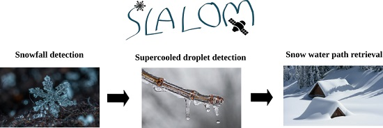
3.1. Snowfall Detection

For the snow detection module, we used the random forest algorithm to predict snowfall occurrence. The training dataset was comprised of 408,254 observations, with 38,331 2CSP-defined snowfall events. In order to build an optimal random forest model, we sought the best combinations of input variables, associated with the 13 GMI radiometer channels, in order to obtain the most reliable predictions. The input variables tested were sea ice concentration, T2m, TPW, the 4 first principal components of the vertical profiles of temperature, specific humidity and relative humidity, snow cover, and land-sea flag. Specifically, we selected 2000 random combinations of input variables and discarded those which were systematically associated with the lowest predictive scores. The optimal random forest chosen was built with the following input variables: T2m, TPW, the 4 first principal components of the vertical profiles of temperature, specific humidity and relative humidity, together with the 13 GMI radiometer channels. It should be noted that surface type variables were systematically associated with the lowest predictive scores in the selection process. This reveals that, by exploiting all GMI channels at the time of the overpass, the random forest itself can combine the information related to the surface conditions (deriving it from the low frequency channels) and the atmospheric variables (e.g., T2m and TPW) with the cloud vertical structure (i.e., presence or absence of snowfall). It should also be noted that, while 2CSP uses ERA-Interim temperature profiles to determine the phase of the detected precipitation, the SLALOM snowfall detection module uses the ERA-Interim temperature profile (together with the variables already listed) to detect snowfall occurrence. We evaluated the impact of the decision tree number of which the random forest (up to 1000 decision trees) is composed on the prediction skill. A 300 decision trees limit was adopted, since the predictive skill does not improve significantly over this number. The output of the snowfall detection module gives a probability of snowfall occurrence at the GMI high-frequency channel resolution, which is then used as an input for the second module (applied only to snowfall pixels) to detect supercooled droplets.

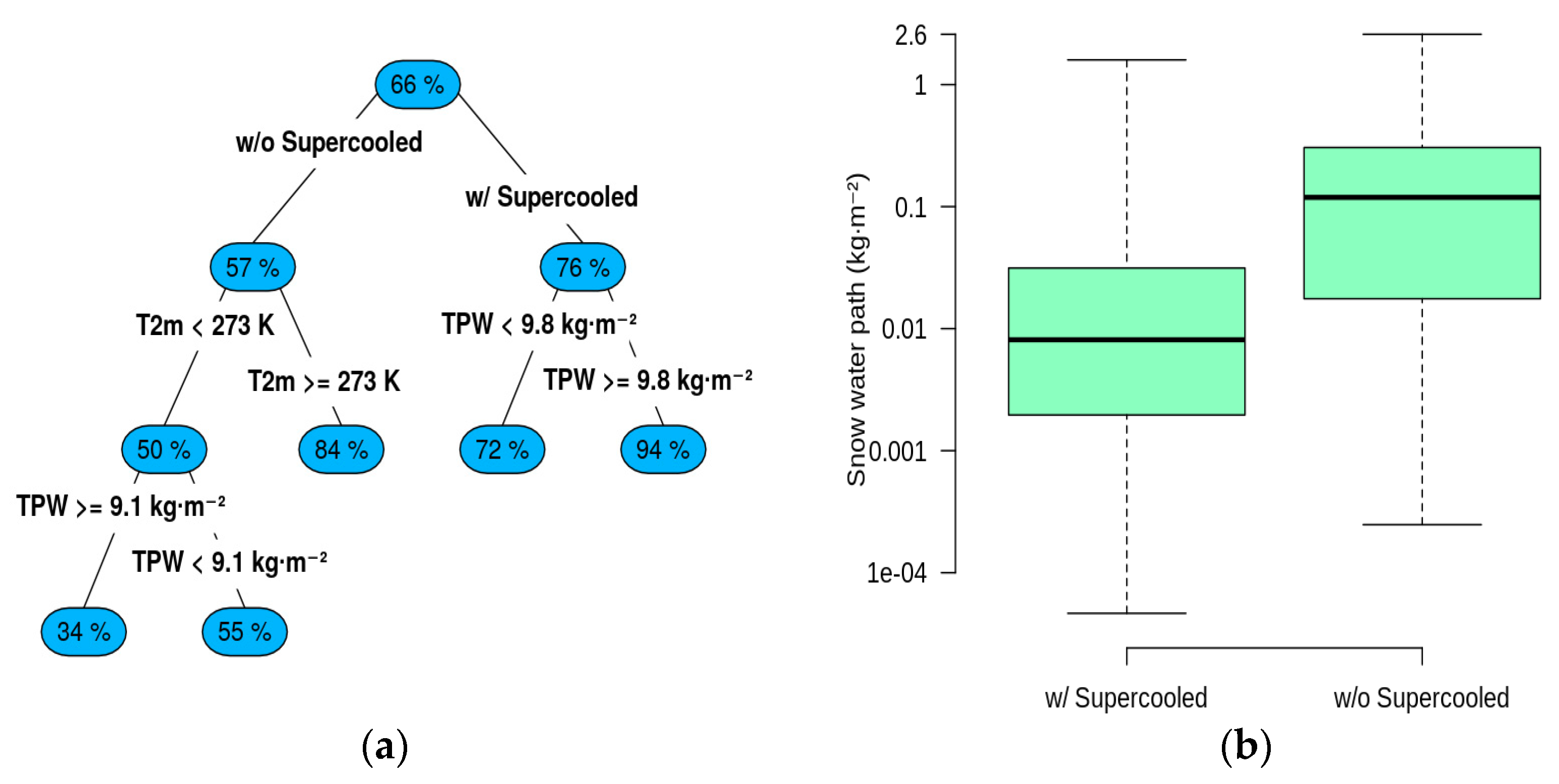
3.2. Supercooled Droplets Detection

Supercooled droplets detection is also based on a random forest approach. Note that, as opposed to Panegrossi et al. [43], we did not consider embedded supercooled droplet cases in the training dataset. Indeed, Panegrossi et al. [43] showed that the strongest impact of supercooled droplets on the measured TBs in the presence of snowfall is found when the supercooled droplets occur at the top of snow clouds. Conversely, the impact of supercooled droplets embedded in the cloud is reduced. The training dataset is the same as that for the snowfall detection module, except that it excludes any embedded supercooled droplet cases. Specifically, it contains 397,033 observations: 10,783 snowfall cases without supercooled droplets and 16,327 snowfall cases with supercooled droplets on top of the cloud. The optimal random forest is similar to the snow detection module, with the same input variables, i.e., T2m, TPW, the vertical profiles of temperature, specific humidity and relative humidity, all 13 GMI channels and 300 decision trees. The output of the supercooled droplet detection module gives a probability of supercooled droplet occurrence at the GMI high-frequency channel resolution, which is then used as an input for the SWP retrieval module.

3.3. SWP Retrieval

In this last module, we sought to infer SWP associated with snowfall using GMI high frequency channel observations. As GMI high frequency channels provide vertically integrated measurements of the atmosphere, the signal of TBs in the presence of snowfall is related to SWP. However, the relationship between SWP and GMI TBs is strongly affected by environmental conditions. Thus, it appeared meaningful to develop an SWP retrieval model that adapts to these conditions. With this aim, we first used a decision tree to split the observations into subsets using the following input variables: T2m, TPW, supercooled occurrence flag and the low frequency GMI channels (i.e., 10.65 H&V, 18.7 H&V, 23.8 V, and 36.5 H&V). We ensured that each subset contained at least 300 observations in order to keep a significant number of points in every subset for the regression procedure. Then, for each of these subsets, we performed a segmented multi-linear regression of SWP as a function of high frequency channel TBs (89 H&V, 166 H&V, 183.31 ± 7, and 183.31 ± 3). Thus, this approach provides a different model for each of the defined subsets, each one of them being adapted to a specific environmental condition.

4. Algorithm Evaluation

We evaluated the predictive capabilities of the algorithm using an independent dataset (i.e., distinct from the training dataset), populated with a random selection of 20% from the observations of the initial dataset (9839 snowfall cases and 102,064 no-snowfall cases). The snowfall and supercooled detection are evaluated using the Probability of Detection (POD), False Alarm Ratio (FAR) and Heidke Skill Score (HSS) metrics [55]:

$$\mathrm{Heidke} \mathrm{Skill} \mathrm{Score} \left(\mathrm{HSS}\right)=\frac{2\ast \left(h\ast cn-fa\ast m\right)}{\left(h+m\right)\ast \left(m+cn\right)+\left(h+fa\right)\ast \left(fa+cn\right)}$$

(1)

where h is the hits (both prediction and reference detect an event), cn is the correct negative (prediction and reference do not detect an event), m is the misses (prediction does not detect any event, but reference does) and fa is a false alarm (prediction detects an event, but reference does not). A high POD means that a high proportion of events were correctly predicted, while a high FAR means that a high proportion of predicted events did not occur. HSS combines h, cn, m and fa to assess the prediction skill.

The SWP retrieval module was evaluated using the Pearson correlation coefficient (r), relative bias (Bias) and root mean square error (RMSE) between the predicted and reference datasets. We also computed the SWP fractional standard error percentage (FSE%), which is defined as follows:

$$\mathrm{FSE}\%=\frac{100\ast \mathrm{RMSE}}{<\mathrm{SWP}>}$$

(2)

where <SWP> is the mean SWP from 2CSP.

Each module has been evaluated independently of the results of the others, e.g., for the supercooled detection module, we considered cases in which snow is detected by the 2CSP, rather than using the outputs of the snow detection module. This assessment strategy ensures that the skill evaluation of each module does not include errors caused by other modules. Obviously, in the operational version of the algorithm (and for the case studies presented in this study), the outputs of the three modules are combined. Therefore, the full SLALOM algorithm, combining the results of the 3 modules, is also evaluated (Section 5.4). The evaluation has been conducted for the whole test dataset and for the following surface types: Open sea, sea ice (sea ice concentration > 90%) and land. Land pixels in the coincident dataset are frozen or snow covered in 88% of the snowfall cases, according to T2m from the GPM-CPR dataset.

5. Results

5.1. Snowfall Detection Module

The snowfall detection module, evaluated on the test dataset, reveals a POD of 0.83, with a FAR of 0.12 and a HSS of 0.84. These statistics are rather similar among surface types: A POD of 0.83, 0.80 and 0.87, a FAR of 0.1, 0.14 and 0.1, and an HSS of 0.85, 0.82 and 0.84 for land, open sea and sea ice, respectively. These results highlight that the performance of the snow detection module does not depend on the surface type.

The sensitivity of the detection module on the 2CSP SWP magnitude is evaluated in Figure 3a. In this Figure, the test dataset is binned as a function of 2CSP SWP and, for each bin, the ratio of the number of missed snow events to the total number of snow events is computed. The percentage of missed snowfall events ranges from 55%, for the lowest SWP given by the 2CSP product (i.e., 3.7 × 10⁻⁵ kg·m⁻²), to less than 10% above 0.02 kg·m⁻². We conducted a similar analysis to evaluate the sensitivity of the snowfall detection module to the surface snowfall rate (not shown). It was revealed that the snow detection module misses 58% of snowfall events, when the surface snowfall rate is about 1 × 10⁻³ mm/h, and less than 10% when the surface snowfall rate exceeds 0.05 mm/h. These findings highlight the high sensitivity of the snow detection module, even for light snowfall events. In order to characterize the cases for which the SLALOM snowfall detection module fails, we computed a decision (regression) tree (Figure 3b). This tool allowed us to identify the environmental variables that explain the percentage of misses by hierarchically partitioning the observations. Thus, in Figure 3b, each leaf (box) contains only a fraction of observations, except for the top box, which contains all the observations. Labels on leaves represent the mean percentage of misses, and the names of variables and inequalities written on branches (black lines) indicate the variable and thresholds chosen to split observations. For each leaf, the tree algorithm selected the most appropriate variables among T2m, TPW, SWP, surface type, and the presence of supercooled droplets for partitioning observations. Thus, in Figure 3b, the average percentage of misses of all observations is 17.1% (top box), and the first variable chosen by the tree to split the observations is SWP. We ensured that each final leaf (bottom box) of the tree contained at least 300 observations in order to obtain reliable results. Results show that the percentage of missed snowfall occurrence reaches 41.4% when SWP is below 3 × 10⁻³ kg·m⁻² while it is 10.3% when SWP is above 3 × 10⁻³ kg·m⁻². In addition, the percentage of misses is much higher when T2m exceeds 275 K (44.2% versus 8.8%), as shown in Figure 3b. This can be explained by the fact that when T2m is greater than 273 K, the occurrence of mixed precipitation increases and, when the liquid fraction becomes greater than 15%, the 2CSP product sets the snowfall rate to zero. However, in these cases, GMI channels are still sensitive to melting snow, and this could explain SLALOM detection difficulties in these situations.

5.2. Supercooled Droplets Detection Module

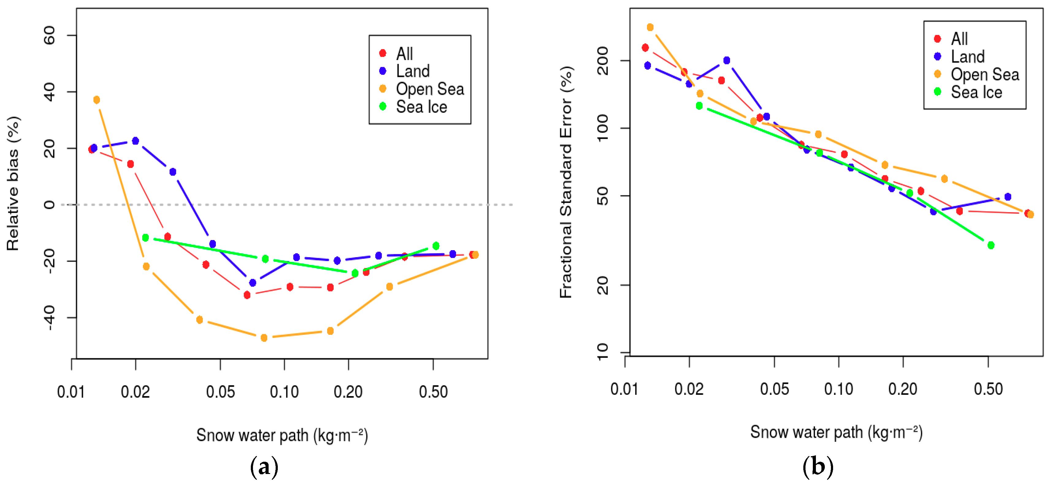
The supercooled detection module shows a POD of 0.97, an FAR of 0.05 and an HSS of 0.89. Once again, the results are rather similar for each surface type: For land (open sea, sea ice), the POD is 0.95 (0.98, 0.97), the FAR is 0.07 (0.04, 0.05) and the HSS is 0.87 (0.9, 0.9). These results illustrate the skill of the random forest approach in distinguishing between snowfall cases with and without supercooled droplets.

The decision tree of the missed and false positive supercooled detection is shown in Figure 4. Each final leaf contains at least 300 observations, and the percentage of missed and false positive supercooled detection is partitioned as a function of T2m, TPW, SWP and surface type. The most significant variable chosen to explain the percentage of missed supercooled droplets is TPW. When TPW is below 2.4 kg·m⁻², the module fails to detect supercooled droplets in 11% of cases. These results, unsurprisingly, show that very dry conditions complicate supercooled droplet detection.

5.3. Snow Retrieval

The skill of the retrieval algorithm, globally and for each surface type, is shown in

Table 1. Comparison of SWP observations from CPR, with SWP predictions for the complete evaluation dataset (All) over land, open sea and sea ice.

Surface	Correlation	Bias	RMSE
All	0.88	−16%	0.1 kg∙m−2
Land	0.85	−13%	0.1 kg∙m−2
Open Sea	0.88	−21%	0.12 kg∙m−2
Sea ice	0.92	−15%	0.08 kg∙m−2

. The correlation between the predicted and observed SWP is 0.88, the relative bias is −16% and the RMSE is 0.10 kg·m⁻². The results are better over sea ice (r = 0.92, Bias = −15% and RMSE = 0.08 kg·m⁻²) than over open sea and land surfaces (r = 0.88 and 0.85, Bias = −21% and −13%, and RMSE = 0.12 and 0.1 kg·m⁻²).

We also investigated the sensitivity of the relative bias and fractional standard error percentage (FSE%) to SWP (Figure 5). The scores have been computed by binning observations as a function of SWP. The relative bias decreases from about 20%, for low SWP (<0.02 kg·m⁻²), to about −30%, for SWP of 0.05 kg·m⁻², and then remains around −20% for SWP higher than 0.05 kg·m⁻². Once again, the results are better over sea ice, with a relative bias constantly between −10 and −20%, while it decreases from 40% to −40% for open sea. The FSE% decreases from 200% at 0.01 kg·m⁻² to about 40% at 1 kg·m⁻². It shows a similar pattern for every surface type below 0.05 kg·m⁻², and, for SWP over 0.05 kg·m⁻², the prediction over open sea shows higher values (around 40% at 1 kg·m⁻²) compared to sea ice (30% at 0.5 kg·m⁻²). Land has an intermediate behavior.

A decision tree, with the absolute value of the difference between predicted and observed SWP, normalized by the observed SWP, is shown in Figure 6. Every final leaf contains at least 300 observations, and partitioning variables are T2m, TPW, presence of supercooled droplets and surface type. Note that we retained only cases for which SWP is greater than 0.01 kg·m⁻². First, the normalized difference is overall lower when no supercooled droplets are present (i.e., left part of the tree). In addition, if T2m is lower than 273 K, and TPW is higher than 6.7 kg·m⁻², the average normalized difference is minimized (34%). These conditions are very favorable for snow retrievals, since the snow scattering signal is not attenuated by the supercooled droplets. Furthermore, temperatures below freezing point prevent the presence of melting snow and rain that can contaminate the snow radiative signature, while higher TPW reduces any surface contamination. On the right part of the tree, which contains cloud top supercooled droplet occurrences, the worst case is found when TPW is high (94% of normalized difference percentage). It is somewhat surprising that, when no supercooled droplets are present, a high humidity is favorable for accurately retrieving snow, while when supercooled droplets are present, a high humidity is less favorable to the retrieval of snow. This TPW and supercooled water relationship might be explained by the fact that snow events with supercooled droplets are usually associated with lower SWP values. Indeed, the median value of SWP when supercooled droplets occur (about 0.01 kg·m⁻²) is more than ten times lower than without supercooled droplet occurrence (about 0.12 kg·m⁻²), as shown in Figure 6b. Therefore, under these conditions, detecting weak snowfall could be more difficult, because water vapor and cloud droplet emission obscure the weak scattering signal.

5.4. Full Algorithm Evaluation and Sensitivity Test

In the previous sections we evaluated each module output independently. In this section, we evaluate the full SLALOM algorithm, combining the results of the 3 modules. Additionally, we included the embedded supercooled droplet cases in this evaluation (while they have not been used for the algorithm training). We also analyzed the sensitivity of the model by evaluating its performance in two experiments: (i) Without supercooled droplet detection and (ii) without using environmental conditions (i.e., only brightness temperatures).

In comparison to observations, global predictions have a correlation of 0.86, a relative bias of −20% and RMSE of 0.04 kg·m⁻², as shown in

Table 2. Comparison of SWP observations from CPR, with SWP predictions for the full SLALOM algorithm (SLALOM), without taking into account supercooled droplets occurrence (SLALOM w/o Sc) and environmental conditions (SLALOM w/o Env).

Configuration	Correlation	Bias	RMSE
SLALOM	0.86	−20%	0.04 kg∙m−2
SLALOM w/o Sc	0.86	−18%	0.04 kg∙m−2
SLALOM w/o Env	0.61	−49%	0.13 kg∙m−2

. Supercooled droplet detection does not have an effect on predictions, meaning that even if supercooled droplets can be detected accurately by SLALOM (Section 5.2), it does not improve the overall SWP retrieval. This could mean that the SWP retrieval module is not able to precisely retrieve SWP when supercooled droplets occur, even if they are appropriately flagged by the supercooled detection module. This interpretation is supported by the fact that the correlation and relative bias (between observations and predictions) are 0.73 and −32% when supercooled droplets are present but reach 0.86 and −16% when no supercooled droplets are present. The fact that supercooled droplets are often associated with a low SWP (Figure 6b) could explain the difficulty of fitting the model to these cases. The importance of considering environmental variables for precisely retrieving SWP is revealed in Table 2. If the model is trained without using environmental conditions, the correlation decreases to 0.67, the relative bias increases to −49% and RMSE increases to 0.13 kg·m⁻².

6. Applications of SLALOM Algorithm

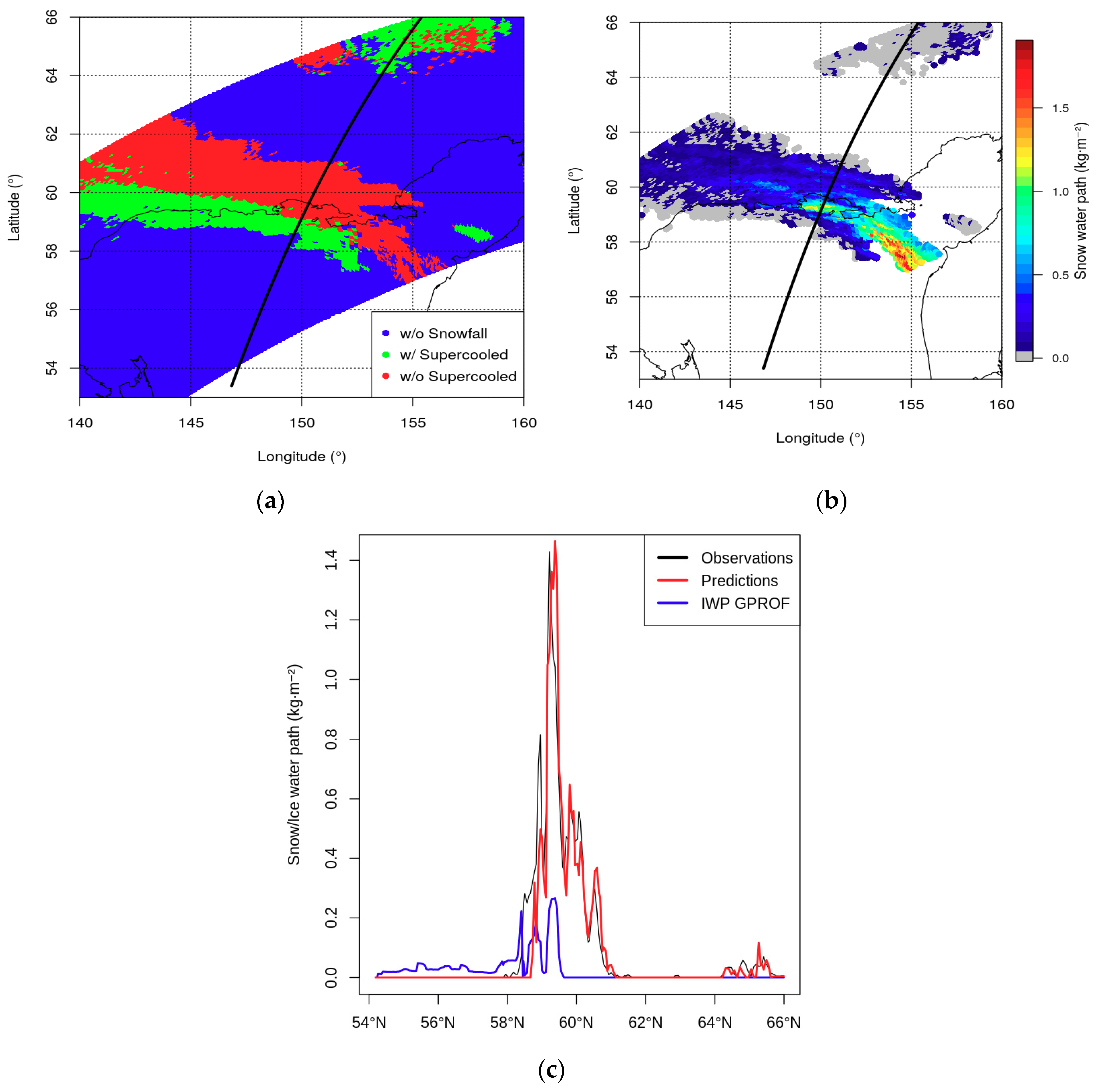
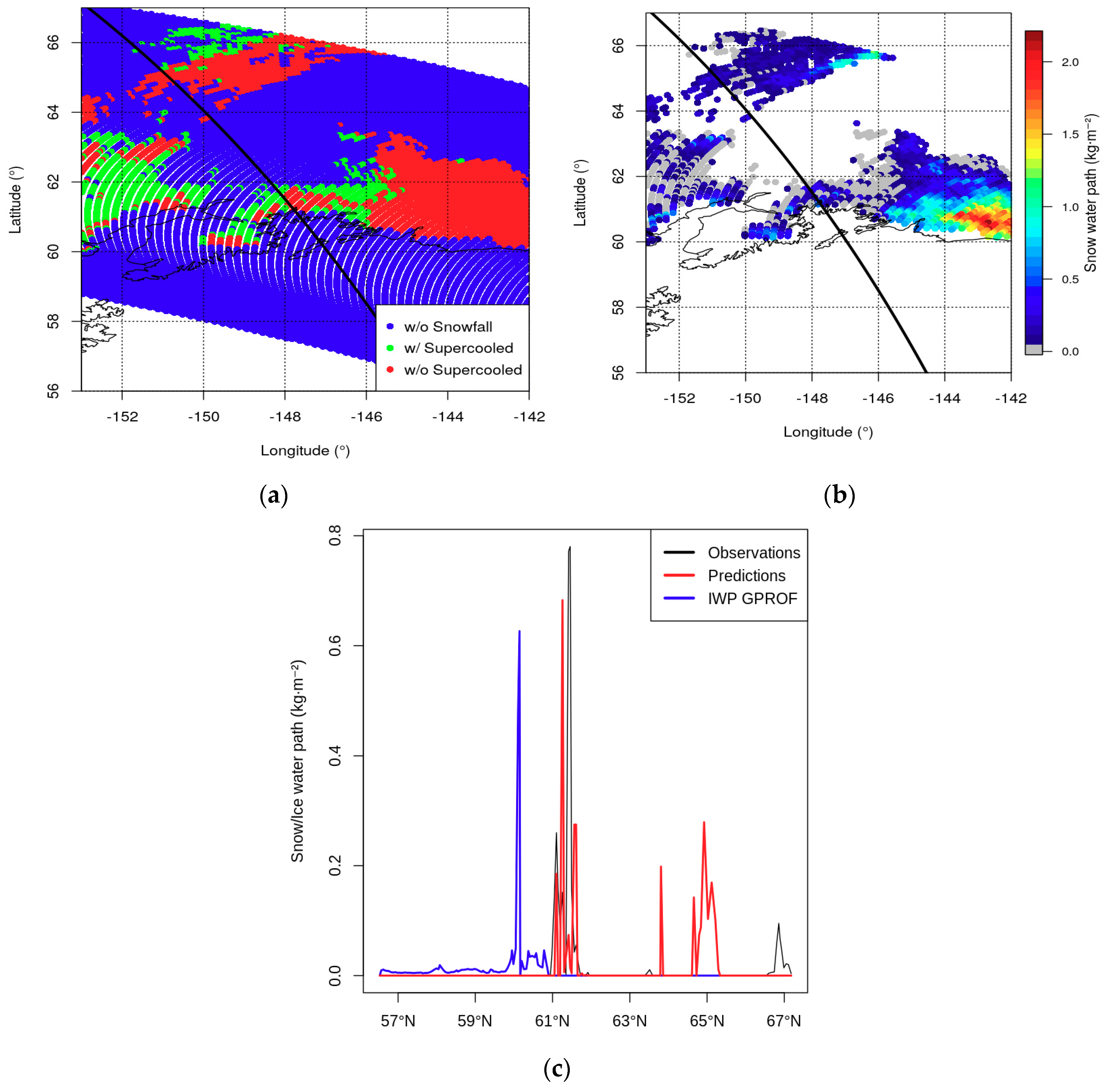
In the two following sections, we highlight some applications of the SLALOM algorithm. First, we used SLALOM to retrieve the snow water path in the three case studies, described in detail in Panegrossi et al. [43]. These case studies have been chosen by Panegrossi et al. [43], since they represent three distinct and somewhat complex snow situations that can be found at around 60° latitude. They allowed us to evaluate the skill of the algorithm in cases of complex meteorological and environmental conditions. Secondly, we built a 0.1° × 0.1° map of snowfall occurrence from May 2014 to May 2016 in order to illustrate the potential of the SLALOM algorithm for climatological analyses.

6.1. Case Studies

The first case study took place on 30 April 2014 in Eastern Siberia and is associated with an extended frontal system. A maximum SWP of 1.4 kg·m⁻² is estimated along the CloudSat track (Figure 7c). The frontal structure (around 60°N) is well captured by the snow and supercooled detection modules (Figure 7a). This reveals that the front is composed of a snowy region without supercooled droplets (in red) and, on the southern part of this region, a snowy region with supercooled droplets. The evaluation of the predictions along the CloudSat track shows that the snow detection module performs well in 85% of cases (here 85% is the ratio of the number of hits and correct negatives to the total number of cases) and, in cases where snowfall has been detected successfully, the supercooled detection module was correct in 90% of cases (i.e., the sum of cases with true supercooled droplets detection and true snowfall without supercooled droplets detection). The SWP module predicts values up to 1.89 kg·m⁻², with the most intense values in the southeastern part of the front (Figure 7b). SWP predictions also show very weak patches (<0.1 kg·m⁻²) on the northern part of the front. SWP observations and predictions match very well in terms of the pattern and magnitude along the CloudSat track, as highlighted in Figure 7c. We also included the ice water path from GPROF (IWP) in Figure 7c. Note that a quantitative comparison with 2CSP or SLALOM is not possible here, since SWP and IWP are different variables (see the conclusion for details). In addition, GPROF does not retrieve IWP over snow covered surfaces (e.g., above 60°N in this case). The highest values of IWP are found where snowfall is detected by 2CSP (with a maximum of 0.25 kg·m⁻² at around 59.5°N).

The second case study is an orographic precipitation event that occurred on 14 December 2014 in Alaska (Figure 8). Unfortunately, the CloudSat track does not cross the most intense part of this snow event, and very low values of SWP are estimated by 2CSP. Predictions show snowfall occurrences with and without supercooled droplets along the coast and in the northern region. SWP predictions show some large values (more than 2 kg·m⁻²) on the eastern part of the region, along the coast (Figure 8b). The evaluation of predictions along the CloudSat track show that, even if the SLALOM algorithm successfully detects snow in the coastal region (around 61°N), predicted SWP does not match observations well and, in addition, several weak SWP peaks (<0.2 kg·m⁻²) are predicted in the north of the region but are not observed. The bad performance of the algorithm in this case is probably related to extremely dry conditions, with the very low TPW observed inland (lower than 5 kg·m⁻²), and to the very weak scattering signal, associated with the light snowfall along the CloudSat track, as evidenced by Panegrossi et al. [43]. It is worth noting, however, the ability of SLALOM to provide SWP estimates over the full GMI swath, including the intense snowfall region that is missed by CloudSat. IWP shows a peak of 0.6 kg·m⁻² at 60°N, while SWP is zero. This could mean that an ice cloud occurred in this region but did not produce snowfall. For latitudes higher than 61°N, IWP is not retrieved because the ground is snow-covered.

The last investigated case is a synoptic snowfall event that occurred over the Labrador Sea on 27 March 2014. This case is characterized by the transition from open sea to sea ice at around 61°N–58°W. A large region of snowfall is predicted south of 61°N nearly without the occurrence of supercooled droplets (Figure 9a). The snow and supercooled detection modules perform very well (87% and 94% of good classification). SWP predictions show a large region with moderate SWP values ranging from 0.5 to 1.3 kg·m⁻² on the eastern part of the region and weaker SWP elsewhere (Figure 9b). The SWP retrieval module also performs well in this case, as it reproduces rather accurately the pattern given by CPR observations. IWP decreases from 0.2 kg·m⁻² at 57° N to 0 kg·m⁻² for latitudes above 61°N.

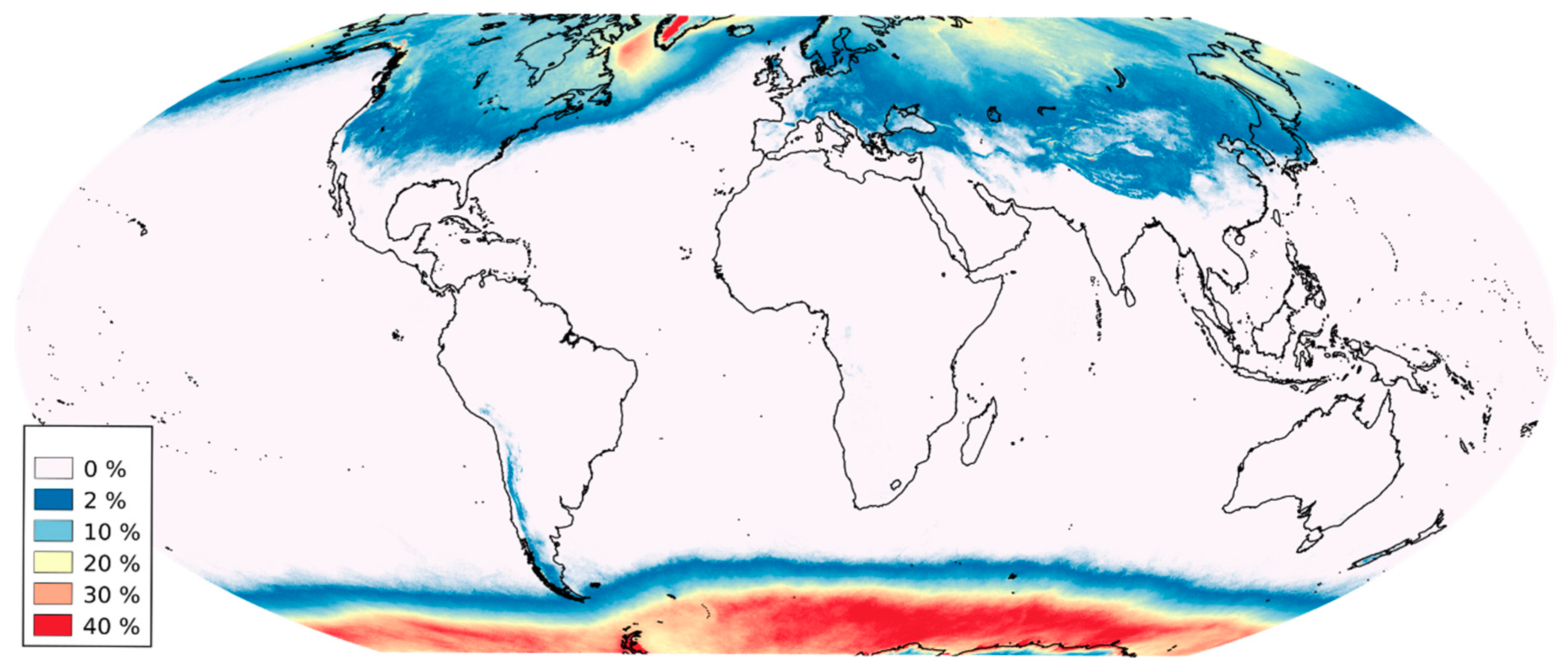
6.2. Climatology of Snowfall Occurrence

The snowfall percentage of occurrence, as given by the snow detection module of SLALOM from May 2014 to May 2016, is shown in Figure 10. For each of GMI orbits between those dates, we applied the snowfall detection module and identified snowfall cases. Then, we binned these detections on a 0.1° × 0.1° grid and normalized it by the total number of GMI observations in each pixel of this grid. For computing optimization reasons, we used here a simplified version of the algorithm to build this climatology, i.e., we did not use vertical profiles of atmospheric variables in the snowfall detection module. The Antarctica coast is the region with the highest occurrence of snowfall, with values reaching 40% in some areas. It is interesting to note the step decrease of snow occurrence as one moves away from the Antarctica coast. In the Northern Hemisphere, the situation is more complex due to the presence of continental regions. The maximum is found over Greenland, with values over 40% and values of about 30% in the Labrador Sea. Siberia, Canada and the eastern side of continents show an occurrence between 2 and 20%, with local variability. Europe and the western side of continents have a snow occurrence lower than 5% of time. Finally, mountain ranges, such as the Himalayas, the Andes, the Alps and the Rocky Mountains show occurrences that can exceed 20%. These patterns match very well those identified at a lower resolution by Kulie et al. [11] and Behrangi et al. [4], using CloudSat CPR observations, and Adhikari et al. [56], using a GPM Dual-frequency Precipitation Radar.

7. Discussion and Conclusions

In this paper, we described and evaluated a new algorithm, named SLALOM (Snow retrievaL ALgorithm fOr gMi), that is able to detect snowfall and to retrieve the associated snow water path (SWP). It is tuned for the GPM Microwave Imager (GMI) but can be adapted to other passive microwave radiometers. SLALOM is trained and evaluated using coincident measurements by the CloudSat Cloud Profiling Radar (CPR) and CALIPSO Cloud-Aerosol Lidar with Orthogonal Polarization (CALIOP). This algorithm is composed of 3 modules: Snowfall detection, supercooled droplet detection and SWP retrieval. It is designed to take into account the impact of environmental conditions (including the occurrence of supercooled droplets) on GMI sensitivity to snowfall and thus to obtain an optimal estimation of SWP. Evaluation of the algorithm reveals that all modules have good skill. Specifically, the snow detection POD is 0.83, with a FAR of 0.12, and supercooled detection shows a POD of 0.97, with a FAR of 0.05. Overall, SWP retrieval shows a correlation of 0.86, a relative bias of −18% and a root mean square error of 0.04 kg·m⁻². In addition, results show that the SLALOM algorithm is able to detect light snowfall, even if it still misses 55% of the lightest events. We also showed that SLALOM is less efficient in cases of mixed phase precipitation, supercooled droplet occurrence, low humidity and low SWP, and we identified the essential role of environmental variables for a meaningful retrieval of SWP. We applied the SLALOM algorithm to three different meteorological situations (frontal snowfall, orographic snowfall and synoptic snowfall). The algorithm performs very well in the first and the third situations, but it has more difficulty in retrieving snowfall in the orographic snowfall situation, which was characterized by dry conditions and a low SWP, according to 2CSP. Finally, we computed a global climatology of snowfall occurrence from May 2014 to May 2016, with a 0.1° × 0.1° resolution. This shows a very good consistency with lower resolution climatologies using CloudSat CPR [4,11].

Overall, these results highlight the high efficiency of the SLALOM algorithm for every surface type. In particular, the high sensitivity of snow detection by the SLALOM algorithm, even for light snowfall, is an important asset, as many studies pointed out that most snow events are associated with very light snowfall rates at high latitudes [9,11,13]. In addition, the snowfall and supercooled detection modules can be exploited to document the water phase at the global scale. As illustrated in this paper, the algorithm outputs can be useful for climatic studies related to the water cycle as well as case study analyses, especially in regions where in-situ measurements are not available.

Interestingly, our results illustrate the limited impact of supercooled droplet detection on SWP retrieval accuracy. The reason might be that the supercooled droplet occurrence is often associated with a low SWP, as shown in Section 5.3. Thus, even if the SLALOM algorithm does not perform as well in supercooled droplet cases, the overall error remains small. Therefore, the accurate detection of supercooled mixed phase clouds for SWP retrieval might not be as crucial as it was initially thought to be. In the future, it could also be worthwhile to evaluate the minimum SWP detectable for every GMI channel when supercooled droplets are present, following work of Kneifel et al. [40]. To this end, we could perform idealized radiative transfer simulations of mixed phase clouds and identify the SWP threshold for which the scattering effects exceed cloud top supercooled droplet emission.

Several limitations of the SLALOM algorithm need to be highlighted. First, SLALOM fully relies on the 2C-SNOW-PROFILE (2CSP) product and is therefore subject to the limitations of the 2CSP product. The main limitation is due to the fact that 2CSP does not provide measurements close to the surface. Thus, it misses an important layer of snowfall and underestimates the total SWP. On the other hand, ground clutter is sometimes not appropriately corrected in complicated terrain (see [9,13]), thus leading to artificially high snow content. Another important limitation lies in the fact that 2CSP SWP is subjected to high uncertainties due to the difficulties in quantifying SWP using a single frequency instrument, such as CPR. Indeed, CPR does not provide enough independent information on snow microphysics to be able to connect measured reflectivity to a unique snowfall rate. Thus, the inversion problem is not fully constrained, which necessitates the use of parameterizations in estimating the snowfall rate from measured reflectivity, implying uncertainties in snowfall estimates [57]. Another difficulty comes from melting snow events. When the liquid fraction is higher than 15%, 2CSP does not retrieve snowfall (these are therefore considered no-snowfall cases). However, the high frequency GMI channels are affected by melting snowfall, even if the liquid fraction is higher than 15%, which can create discrepancies between both SLALOM and 2CSP. In addition, coincidences between CPR and GMI are unevenly distributed (Figure 1), which can also affect the overall predictions.

Secondly, the SLALOM algorithm design itself has some limitations. For instance, the snow retrieval module assumes a segmented multi-linear relationship between high frequency brightness temperatures and SWP. It is probable that a more realistic (but complex) relationship could be found and could reduce SWP retrieval uncertainties. In addition, we only trained the algorithm using supercooled droplets on top of the cloud and discounted supercooled droplet layers embedded within the cloud. However, embedded supercooled layers frequently occur in the coincident database (about 30% of time). Depending on the position in the cloud, supercooled droplet layers can mask more or less of the snow scattering signal. Considering the embedded cases could improve the algorithm predictions.

Previous studies on the GMI snowfall detection capability assessment [18,26,33,43] demonstrate that GMI has great potential for snowfall observation. In this work, we have shown that, through the exploitation of all 13 GMI channels and the optimal use of ancillary variables describing the atmospheric conditions (and no ancillary information on the background surface conditions), SLALOM is able to predict snowfall occurrence and SWP, with a very good agreement with the Cloudsat 2CSP product, and has the advantage of ensuring a much larger spatial coverage, corresponding to the GMI swath. In spite of some of the limitations already mentioned, SLALOM can be applied effectively in case studies as well as in climatology analysis. SLALOM will be further developed to provide the surface snowfall rate and incorporated in the global precipitation retrieval algorithm for GMI, developed recently within the EUMETSAT Satellite Application Facility on support to Operational Hydrology and Water Management (H SAF) program [58]. In the future, studies similar to that of Panegrossi et al. [43], based on the use of experimental datasets built from coincident observations by Cloudsat and other passive microwave radiometers in the GPM constellation (conical and cross-track scanning), will be carried out, and approaches similar to SLALOM will be developed to extend snowfall detection and retrieval to higher latitudes, and they will have a global coverage of snowfall by the passive microwave radiometer constellation. In addition, a comparison of the SLALOM product with other operational products, such as GPROF, will be conducted. There are some important factors to be considered in order to conduct such comparison. One is the difficulty in finding high-quality and independent snowfall observations and estimates to be used as the “truth”. Then, there are product differences, often difficult to reconcile, that can derive from different sources: the method used to determine the phase of the precipitation on the surface; the differences in orbits and swath widths; instrumentation differences (channel assortment and resolution); and differences in the algorithm formulation and assumptions, which are oftenf not well understood [59]. Review papers, similar to that of Levizzani et al. [3], summarizing the main snowfall retrieval techniques currently available, are thus strongly needed.

References

1. Knowles, N.; Dettinger, M.D.; Cayan, D.R. Trends in snowfall versus rainfall in the Western United States. J. Clim. 2006, 19, 4545–4559. [Google Scholar] [CrossRef]
2. Feng, S.; Hu, Q. Changes in winter snowfall/precipitation ratio in the contiguous United States. J. Geophys. Res. Atmos. 2007, 112, D15109. [Google Scholar] [CrossRef]
3. Levizzani, V.; Laviola, S.; Cattani, E. Detection and measurement of snowfall from space. Remote Sens. 2011, 3, 145–166. [Google Scholar] [CrossRef]
4. Behrangi, A.; Christensen, M.; Richardson, M.; Lebsock, M.; Stephens, G.; Huffman, G.J.; Bolvin, D.; Adler, R.F.; Gardner, A.; Lambrigtsen, B.; et al. Status of high-latitude precipitation estimates from observations and reanalyses. J. Geophys. Res.-Atmos. 2016, 121, 4468–4486. [Google Scholar] [CrossRef] [PubMed]
5. Skofronick-Jackson, G.M.; Kim, M.J.; Weinman, J.A.; Chang, D.E. A physical model to determine snowfall over land by microwave radiometry. IEEE Trans. Geosci. Remote Sens. 2004, 42, 1047–1058. [Google Scholar] [CrossRef] [Green Version]
6. Skofronick-Jackson, G.M.; Johnson, B.T.; Munchak, S.J. Detection thresholds of falling snow from satellite-borne active and passive sensors. IEEE Trans. Geosci. Remote Sens. 2013, 51, 4177–4189. [Google Scholar] [CrossRef]
7. Stephens, G.L.; Vane, D.G.; Boain, R.J.; Mace, G.G.; Sassen, K.; Wang, Z.E.; Illingworth, A.J.; O’Connor, E.J.; Rossow, W.B.; Durden, S.L.; et al. The cloudsat mission and the a-train—A new dimension of space-based observations of clouds and precipitation. Bull. Am. Meteorol. Soc. 2002, 83, 1771–1790. [Google Scholar] [CrossRef]
8. Hou, A.Y.; Kakar, R.K.; Neeck, S.; Azarbarzin, A.A.; Kummerow, C.D.; Kojima, M.; Oki, R.; Nakamura, K.; Iguchi, T. The global precipitation measurement mission. Bull. Am. Meteorol. Soc. 2014, 95, 701–722. [Google Scholar] [CrossRef]
9. Kulie, M.S.; Bennartz, R. Utilizing spaceborne radars to retrieve dry snowfall. J. Appl. Meteorol. Climatol. 2009, 48, 2564–2580. [Google Scholar] [CrossRef]
10. Hiley, M.J.; Kulie, M.S.; Bennartz, R. Uncertainty analysis for CloudSat snowfall retrievals. J. Appl. Meteorol. Climatol. 2011, 50, 399–418. [Google Scholar] [CrossRef]
11. Kulie, M.S.; Milani, L.; Wood, N.B.; Tushaus, S.A.; Bennartz, R.; L’Ecuyer, T.S. A shallow cumuliform snowfall census using spaceborne radar. J. Hydrometeorol. 2016, 17, 1261–1279. [Google Scholar] [CrossRef]
12. Chen, S.; Hong, Y.; Kulie, M.; Behrangi, A.; Stepanian, P.M.; Cao, Q.; You, Y.; Zhang, J.; Hu, J.; Zhang, X. Comparison of snowfall estimates from the NASA CloudSat cloud profiling radar and NOAA/NSSL multi-radar multi-sensor system. J. Hydrol. 2016, 541, 862–872. [Google Scholar] [CrossRef]
13. Milani, L.; Kulie, M.S.; Casella, D.; Dietrich, S.; L’Ecuyer, T.S.; Panegrossi, G.; Porcù, F.; Sanò, P.; Wood, N.B. CloudSat snowfall estimates over Antarctica and the Southern Ocean: An assessment of independent retrieval methodologies and multi-year snowfall analysis. Atmos. Res. 2018, 213, 121–135. [Google Scholar] [CrossRef]
14. Casella, D.; Panegrossi, G.; Sano, P.; Marra, A.C.; Dietrich, S.; Johnson, B.T.; Kulie, M.S. Evaluation of the GPM-DPR snowfall detection capability: Comparison with CloudSat-CPR. Atmos. Res. 2017, 197, 64–75. [Google Scholar] [CrossRef]
15. Bennartz, R.; Bauer, P. Sensitivity of microwave radiances at 85–183 GHz to precipitating ice particles. Radio Sci. 2003, 38. [Google Scholar] [CrossRef]
16. Liu, G.; Seo, E.-K. Detecting snowfall over land by satellite high-frequency microwave observations: The lack of scattering signature and a statistical approach. J. Geophys. Res.-Atmos. 2013, 118, 1376–1387. [Google Scholar] [CrossRef]
17. Skofronick-Jackson, G.; Johnson, B.T. Surface and atmospheric contributions to passive microwave brightness temperatures for falling snow events. J. Geophys. Res.-Atmos. 2011, 116, D02213. [Google Scholar] [CrossRef]
18. Gong, J.; Wu, D.L. Microphysical properties of frozen particles inferred from Global Precipitation Measurement (GPM) Microwave Imager (GMI) polarimetric measurements. Atmos. Chem. Phys. 2017, 17, 2741–2757. [Google Scholar] [CrossRef] [Green Version]
19. Liu, G.S.; Curry, J.A. Precipitation characteristics in Greenland-Iceland-Norwegian Seas determined by using satellite microwave data. J. Geophys. Res.-Atmos. 1997, 102, 13987–13997. [Google Scholar] [CrossRef] [Green Version]
20. Kongoli, C.; Pellegrino, P.; Ferraro, R.R.; Grody, N.C.; Meng, H. A new snowfall detection algorithm over land using measurements from the Advanced Microwave Sounding Unit (AMSU). Geophys. Res. Lett. 2003, 30, 1756. [Google Scholar] [CrossRef]
21. Surussavadee, C.; Staelin, D.H. Satellite retrievals of arctic and equatorial rain and snowfall rates using millimeter wavelengths. IEEE Trans. Geosci. Remote Sens. 2009, 47, 3697–3707. [Google Scholar] [CrossRef]
22. Noh, Y.-J.; Liu, G.; Jones, A.S.; Haar, T.H.V. Toward snowfall retrieval over land by combining satellite and in situ measurements. J. Geophys. Res.-Atmos. 2009, 114, D24205. [Google Scholar] [CrossRef]
23. Kongoli, C.; Meng, H.; Dong, J.; Ferraro, R. A snowfall detection algorithm over land utilizing high-frequency passive microwave measurements-Application to ATMS. J. Geophys. Res.-Atmos. 2015, 120, 1918–1932. [Google Scholar] [CrossRef] [Green Version]
24. Kongoli, C.; Meng, H.; Dong, J.; Ferraro, R. A hybrid snowfall detection method from satellite passive microwave measurements and global forecast weather models. Q. J. R. Meteorol. Soc. 2018. [Google Scholar] [CrossRef]
25. You, Y.; Wang, N.-Y.; Ferraro, R. A prototype precipitation retrieval algorithm over land using passive microwave observations stratified by surface condition and precipitation vertical structure. J. Geophys. Res.-Atmos. 2015, 120, 5295–5315. [Google Scholar] [CrossRef] [Green Version]
26. You, Y.; Wang, N.-Y.; Ferraro, R.; Rudlosky, S. Quantifying the snowfall detection performance of the GPM microwave imager channels over land. J. Hydrometeorol. 2017, 18, 729–751. [Google Scholar] [CrossRef]
27. Kummerow, C.D.; Randel, D.L.; Kulie, M.; Wang, N.-Y.; Ferraro, R.; Joseph Munchak, S.; Petkovic, V. The evolution of the Goddard profiling algorithm to a fully parametric scheme. J. Atmos. Ocean. Technol. 2015, 32, 2265–2280. [Google Scholar] [CrossRef]
28. Sims, E.M.; Liu, G. A parameterization of the probability of snow–rain transition. J. Hydrometeorol. 2015, 16, 1466–1477. [Google Scholar] [CrossRef]
29. Skofronick-Jackson, G.; Munchak, S.J.; Ringerud, S.; Petersen, W.; Lott, B. Falling snow estimates from the global precipitation measurement (gpm) mission. In Proceedings of the 2017 IEEE International Geoscience and Remote Sensing Symposium (IGARSS), Fort Worth, TX, USA, 23–28 July 2017; IEEE: New York, NY, USA, 2017; pp. 2724–2727, ISBN 978-1-5090-4951-6. [Google Scholar]
30. Prigent, C.; Aires, F.; Rossow, W.B. Land surface microwave emissivities over the globe for a decade. Bull. Am. Meteorol. Soc. 2006, 87, 1573–1584. [Google Scholar] [CrossRef]
31. Foster, J.L.; Skofronick-Jackson, G.; Meng, H.; Wang, J.R.; Riggs, G.; Kocin, P.J.; Johnson, B.T.; Cohen, J.; Hall, D.K.; Nghiem, S.V. Passive microwave remote sensing of the historic February 2010 snowstorms in the Middle Atlantic region of the USA. Hydrol. Process. 2012, 26, 3459–3471. [Google Scholar] [CrossRef]
32. Turk, F.J.; Haddad, Z.S.; Kirstetter, P.; You, Y.; Ringerud, S. An observationally based method for stratifying a priori passive microwave observations in a Bayesian-based precipitation retrieval framework. Q. J. R. Meteorol. Soc. 2017. [Google Scholar] [CrossRef]
33. Ebtehaj, A.M.; Kummerow, C.D. Microwave retrievals of terrestrial precipitation over snow-covered surfaces: A lesson from the GPM satellite. Geophys. Res. Lett. 2017, 44, 6154–6162. [Google Scholar] [CrossRef]
34. Petty, G. Physical retrievals of over-ocean rain rate from multichannel microwave imagery. 1: Theoretical characteristics of normalized polarization and scattering indexes. Meteorol. Atmos. Phys. 1994, 54, 79–99. [Google Scholar] [CrossRef]
35. Bennartz, R.; Petty, G.W. The sensitivity of microwave remote sensing observations of precipitation to ice particle size distributions. J. Appl. Meteorol. 2001, 40, 345–364. [Google Scholar] [CrossRef]
36. Kulie, M.S.; Bennartz, R.; Greenwald, T.J.; Chen, Y.; Weng, F. Uncertainties in microwave properties of frozen precipitation implications for remote sensing and data assimilation. J. Atmos. Sci. 2010, 67, 3471–3487. [Google Scholar] [CrossRef]
37. Petty, G.W.; Huang, W. Microwave backscatter and extinction by soft ice spheres and complex snow aggregates. J. Atmos. Sci. 2010, 67, 769–787. [Google Scholar] [CrossRef]
38. Kuo, K.-S.; Olson, W.S.; Johnson, B.T.; Grecu, M.; Tian, L.; Clune, T.L.; van Aartsen, B.H.; Heymsfield, A.J.; Liao, L.; Meneghini, R. The microwave radiative properties of falling snow derived from nonspherical ice particle models. Part I: An extensive database of simulated pristine crystals and aggregate particles, and their scattering properties. J. Appl. Meteorol. Climatol. 2016, 55, 691–708. [Google Scholar] [CrossRef]
39. Olson, W.S.; Tian, L.; Grecu, M.; Kuo, K.-S.; Johnson, B.T.; Heymsfield, A.J.; Bansemer, A.; Heymsfield, G.M.; Wang, J.R.; Meneghini, R. The microwave radiative properties of falling snow derived from nonspherical ice particle models. Part II: Initial testing using radar, radiometer and in situ observations. J. Appl. Meteorol. Climatol. 2016, 55, 709–722. [Google Scholar] [CrossRef]
40. Kneifel, S.; Loehnert, U.; Battaglia, A.; Crewell, S.; Siebler, D. Snow scattering signals in ground-based passive microwave radiometer measurements. J. Geophys. Res.-Atmos. 2010, 115, D16214. [Google Scholar] [CrossRef]
41. Wang, Y.; Liu, G.; Seo, E.-K.; Fu, Y. Liquid water in snowing clouds: Implications for satellite remote sensing of snowfall. Atmos. Res. 2013, 131, 60–72. [Google Scholar] [CrossRef]
42. Johnson, B.T.; Olson, W.S.; Skofronick-Jackson, G. The microwave properties of simulated melting precipitation particles: Sensitivity to initial melting. Atmos. Meas. Tech. 2016, 9, 9–21. [Google Scholar] [CrossRef]
43. Panegrossi, G.; Rysman, J.-F.; Casella, D.; Marra, A.C.; Sano, P.; Kulie, M.S. CloudSat-based assessment of GPM microwave imager snowfall observation capabilities. Remote Sens. 2017, 9, 1263. [Google Scholar] [CrossRef]
44. Panegrossi, G.; Rysman, J.-F.; Casella, D.; Sano, P.; Marra, A.C.; Dietrich, S.; Kulie, M.S. Exploitation of GPM/CloudSat coincidence dataset for global snowfall retrieval. In Proceedings of the 2018 IEEE International Geoscience and Remote Sensing Symposium (IGARSS), Valencia, Spain, 23–27 July 2018; IEEE: New York, NY, USA, 2018. [Google Scholar]
45. Draper, D.W.; Newell, D.A.; Wentz, F.J.; Krimchansky, S.; Skofronick-Jackson, G.M. The global precipitation measurement (GPM) microwave imager (GMI): Instrument overview and early on-orbit performance. IEEE J. Sel. Top. Appl. Earth Observ. Remote Sens. 2015, 8, 3452–3462. [Google Scholar] [CrossRef]
46. Skofronick-Jackson, G.; Berg, W.; Kidd, C.; Kirschbaum, D.B.; Petersen, W.A.; Huffman, G.J.; Takayabu, Y.N. Global precipitation measurement (GPM): Unified precipitation estimation from space. In Remote Sensing of Clouds and Precipitation; Andronache, C., Ed.; Springer International Publishing: Cham, Switzerland, 2018; pp. 175–193. ISBN 978-3-319-72583-3. [Google Scholar]
47. Turk, J. CloudSat-GPM coincidence dataset (version 1C). In NASA Technical Report; California Institute of Technology: Pasadena, CA, USA, 2016. [Google Scholar]
48. Xie, X.; Loehnert, U.; Kneifel, S.; Crewell, S. Snow particle orientation observed by ground-based microwave radiometry. J. Geophys. Res.-Atmos. 2012, 117, D02206. [Google Scholar] [CrossRef]
49. Battaglia, A.; Delanoë, J. Synergies and complementarities of CloudSat-CALIPSO snow observations. J. Geophys. Res.-Atmos. 2013, 118, 721–731. [Google Scholar] [CrossRef] [Green Version]
50. Dee, D.P.; Uppala, S.M.; Simmons, A.J.; Berrisford, P.; Poli, P.; Kobayashi, S.; Andrae, U.; Balmaseda, M.A.; Balsamo, G.; Bauer, P.; et al. The ERA-Interim reanalysis: Configuration and performance of the data assimilation system. Q. J. R. Meteorol. Soc. 2011, 137, 553–597. [Google Scholar] [CrossRef]
51. Spreen, G.; Kaleschke, L.; Heygster, G. Sea ice remote sensing using AMSR-E 89-GHz channels. J. Geophys. Res.-Oceans 2008, 113, C02S03. [Google Scholar] [CrossRef]
52. Breiman, L. Random forests. Mach. Learn. 2001, 45, 5–32. [Google Scholar] [CrossRef]
53. Liu, J.; Wu, S.Y.; Zidek, J.V. On segmented multivariate regression. Stat. Sin. 1997, 7, 497–525. [Google Scholar]
54. Breiman, L. Classification and Regression Trees; Routledge: Abingdon, UK, 2017. [Google Scholar]
55. Wilks, D.S. Statistical Methods in the Atmospheric Sciences; Academic Press: Cambridge, MA, USA, 2011; ISBN 978-0-12-385022-5. [Google Scholar]
56. Adhikari, A.; Liu, C.; Kulie, M.S. Global distribution of snow precipitation features and their properties from 3 years of GPM observations. J. Clim. 2018, 31, 3731–3754. [Google Scholar] [CrossRef]
57. Wood, N.B.; L’Ecuyer, T.S.; Heymsfield, A.J.; Stephens, G.L.; Hudak, D.R.; Rodriguez, P. Estimating snow microphysical properties using collocated multisensor observations. J. Geophys. Res. Atmos. 2014, 119, 8941–8961. [Google Scholar] [CrossRef] [Green Version]
58. Sano, P.; Panegrossi, G.; Casella, D.; Marra, A.C.; D’Adderio, L.P.; Rysman, J.-F.; Dietrich, S. The passive microwave neural network precipitation retrieval (PNPR) algorithm for the conical scanning GMI radiometer. Remote Sens. 2018, 10, 1122. [Google Scholar] [CrossRef]
59. Skofronick-Jackson, G.; Kulie, M.S.; Milani, L.; Munchak, S.J.; Wood, N.B.; Levizzani, V. Satellite estimation of falling snow: A global precipitation measurement (GPM) core observatory perspective. Rev. J. Appl. Meteorol. Climatol. (under review).
60. RCoreTeam. R: A Language and Environment for Statistical Computing; RCoreTeam: Vienna, Austria, 2013. [Google Scholar]
61. Fischer, B. rhdf5-HDF5 interface for R. In R# Package Version; RCoreTeam: Vienna, Austria, 2015; Volume 2. [Google Scholar]
62. Pierce, D. ncdf4: Interface to Unidata netCDF (Version 4 or Earlier) Format Data Files. R Package 2012. Available online: http://CRAN. R-project. org/package = ncdf4 (accessed on 31 January 2018).
63. Therneau, T.; Atkinson, B.; Ripley, B. RPART: Recursive Partitioning and Regression Trees. In R Package Version 4.1–10; RCoreTeam: Vienna, Austria, 2015. [Google Scholar]
64. Dowle, M.; Short, T.; Lianoglou, S.; Saporta, R.; Srinivasan, A.; Antonyan, E. Data. Table: Extension of Data. Frame. 2014. Available online: https://cran.r-project.org/web/packages/data.table/index.html (accessed on 31 January 2018).
65. Liaw, A.; Wiener, M. Classification and regression by randomForest. R News 2002, 2, 18–22. [Google Scholar]
66. Kuhn, M.; Wing, J.; Weston, S.; Williams, A.; Keefer, C.; Engelhardt, A. Caret: Classification and regression training. 2016. In R Package Version; RCoreTeam: Vienna, Austria, 2017; Volume 4. [Google Scholar]
67. Hothorn, T.; Hornik, K.; Zeileis, A. Unbiased recursive partitioning: A conditional inference framework. J. Comput. Graph. Stat. 2006, 15, 651–674. [Google Scholar] [CrossRef]
68. Zeileis, A.; Hothorn, T.; Hornik, K. Model-based recursive partitioning. J. Comput. Graph. Stat. 2008, 17, 492–514. [Google Scholar] [CrossRef]
69. Bates, D.; Mächler, M.; Bolker, B.; Walker, S. Fitting linear mixed-effects models using lme4. arXiv. 2014. arXiv Preprint:1406.5823. Available online: https://arxiv.org/abs/1406.5823 (accessed on 31 January 2018).
70. Venables, W.N.; Ripley, B.D. Modern Applied Statistics with S-PLUS; Springer Science & Business Media: New York, NY, USA, 2013; ISBN 978-1-4757-3121-7. [Google Scholar]
71. Zambrano-Bigiarini, M. hydroGOF: Goodness-of-fit functions for comparison of simulated and observed hydrological time series. In R Package Version 0.3-8; RCoreTeam: Vienna, Austria, 2014. [Google Scholar]
72. Ripley, B. Tree: Classification and regression trees. In R Package Version; RCoreTeam: Vienna, Austria, 2005; Available online: http://CRAN.R-project.org/package=tree (accessed on 31 January 2018).
73. Elseberg, J.; Magnenat, S.; Siegwart, R.; Nüchter, A. Comparison of nearest-neighbor-search strategies and implementations for efficient shape registration. J. Softw. Eng. Robot. 2012, 3, 2–12. [Google Scholar]
74. Tierney, L.; Rossini, A.J.; Li, N.; Sevcikova, H. Snow: Simple network of workstations. R Package Version 0.3-3; RCoreTeam: Vienna, Austria, 2008; Available online: http://CRAN.R-project.org/package=snow (accessed on 31 January 2018).
75. Knaus, J. Snowfall: Easier cluster computing (based on snow). In R Package Version; RCoreTeam: Vienna, Austria, 2010; Volume 1. [Google Scholar]
76. Muggeo, V.M. Estimating regression models with unknown break-points. Stat. Med. 2003, 22, 3055–3071. [Google Scholar] [CrossRef] [PubMed]
77. Muggeo, V.M. Segmented: An R package to fit regression models with broken-line relationships. R news 2008, 8, 20–25. [Google Scholar]
78. Adler, D.; Murdoch, D.; Nenadic, O.; Urbanek, S.; Chen, M.; Gebhardt, A.; Bolker, B.; Csardi, G.; Strzelecki, A.; Senger, A. Rgl: 3D visualization using OpenGL. In R Package Version 0.95; RCoreTeam: Vienna, Austria, 2016; Volume 1441. [Google Scholar]
Figure 1. Timeline of several snowfall detection and retrieval algorithms. Box color indicates the instrument for which a given algorithm has been developed.
Remotesensing 10 01278 g001
Figure 2. Zonal distribution of GMI/CPR coincidences: All (grey), snowfall (red), and snowfall with supercooled droplets (blue).
Remotesensing 10 01278 g002
Figure 3. (a) Percentage of missed snowfall occurrence as a function of SWP; and (b) decision tree, with the percentage of missed snowfall occurrences indicated in boxes, and partitioning variables and thresholds indicated on branches.
Remotesensing 10 01278 g003
Figure 4. Decision tree, with the percentage of missed and false positive supercooled occurrence indicated in boxes, and partitioning variables and thresholds indicated on branches.
Remotesensing 10 01278 g004
Figure 5. (a) Relative bias percentage as a function of SWP and surface type; and (b) Fractional Standard Error percentage as a function of SWP and surface type.
Remotesensing 10 01278 g005
Figure 6. (a) Decision tree, with the absolute value of the normalized difference percentage between predicted and observed SWP indicated in boxes, and partitioning variables and thresholds indicated on branches; and (b) Boxplot of observed SWP, with supercooled droplets (left) and without supercooled droplets (right).
Remotesensing 10 01278 g006
Figure 7. Case study of 30 April 2014: (a) Supercooled droplet classification, predicted by SLALOM (blue: Without snow; green: With snowfall and supercooled droplets; red: With snowfall and without supercooled droplets) and the CloudSat track in black; (b) retrieved SWP and the CloudSat track in black; and (c) SWP cross section along the CloudSat track for observations (black), SLALOM predictions (red), and the GPROF ice water path (IWP) (blue).
Remotesensing 10 01278 g007
Figure 8. Same as for Figure 7 but for the 14 December 2014 event.
Remotesensing 10 01278 g008
Figure 9. Same as for Figure 7 but for the 27 March 2014 event.
Remotesensing 10 01278 g009
Figure 10. Snowfall percentage of occurrence, as given by the snow detection module of SLALOM, from May 2014 to May 2016 on a 0.1° × 0.1° grid.
Remotesensing 10 01278 g010