Spectral and Spatial Classification of Hyperspectral Images Based on Random Multi-Graphs


1
College of Information Science and Engineering, Ocean University of China, Qingdao 266100, China
2
Qingdao Key Laboratory of Mixed Reality and Virtual Ocean, Ocean University of China, Qingdao 266100, China
3
Beijing Key Laboratory of Digital Media, School of Computer Science and Engineering, Beihang University, Beijing 100191, China
*
Author to whom correspondence should be addressed.
Remote Sens. 2018, 10(8), 1271; https://doi.org/10.3390/rs10081271
Submission received: 10 July 2018
/
Revised: 5 August 2018
/
Accepted: 9 August 2018
/
Published: 12 August 2018
(This article belongs to the Special Issue Widespread Applications Based on Hyperspectral Technologies from Space)
Abstract
:Hyperspectral image classification has been acknowledged as the fundamental and challenging task of hyperspectral data processing. The abundance of spectral and spatial information has provided great opportunities to effectively characterize and identify ground materials. In this paper, we propose a spectral and spatial classification framework for hyperspectral images based on Random Multi-Graphs (RMGs). The RMG is a graph-based ensemble learning method, which is rarely considered in hyperspectral image classification. It is empirically verified that the semi-supervised RMG deals well with small sample setting problems. This kind of problem is very common in hyperspectral image applications. In the proposed method, spatial features are extracted based on linear prediction error analysis and local binary patterns; spatial features and spectral features are then stacked into high dimensional vectors. The high dimensional vectors are fed into the RMG for classification. By randomly selecting a subset of features to create a graph, the proposed method can achieve excellent classification performance. The experiments on three real hyperspectral datasets have demonstrated that the proposed method exhibits better performance than several closely related methods.

1. Introduction
With the advance of earth observation programs, many hyperspectral sensors with high spectral resolution have been developed, such as NASA’s Airborne Visible/Infrared Imaging Spectrometer (AVIRIS), and NASA’s EO-1 with its hyperspectral instrument Hyperion. The AVIRIS can acquire image data in 224 bands of 10 nm spectral resolution in the reflected visible and near infrared spectrum. The Hyperion can acquire image data in 242 spectral bands at approximately 10 nm spectral resolution. In China, hyperspectral sensors include FY-3A with the Medium-Resolution Spectral Imager (MERSI), Chang’E-1 with the Interferometric Imaging Spectrometer (IIS), and the upcoming GaoFen-5 with the Advanced Hyperspectral Imager (AHSI). More and more remote sensing hyperspectral images are available. Hyperspectral images can obtain hundreds of narrowband spectral channels for the same area, and can provide richer spectral information to support the fine recognition of various land-cover materials. Therefore, hyperspectral images have drawn increasing attention and opened up new remote sensing application fields, such as hydrocarbon detection [1], lake sediment analysis [2], oil reservoir exploration [3], and diseased wheat detection [4], etc. Among these applications, classification of hyperspectral images is well acknowledged as the fundamental and challenging task of hyperspectral data processing. Therefore, hyperspectral image classification has been widely studied in the last two decades [5].
Given a set of observations with known class labels, the basic goal of hyperspectral image classification is to assign a class label to each pixel [6]. Then, the material properties of each pixel can be well described. However, hyperspectral images pose strong classification challenges, such as the well-known Hughes phenomenon. The Hughes phenomenon [7] means that an increase in dimensions of limited training samples will cause a decrease in classification performance [8]. To solve the problem, feature extraction is considered as a critical step in hyperspectral image processing. However, due to the spatial variability of spectral signatures, hyperspectral image feature extraction is widely acknowledged as one of the most challenging tasks in hyperspectral image processing [9,10].
Many existing methods used a series of manually extracted features [11,12,13,14,15,16], which involve massive parameter setting and experts’ experience. Gabor wavelet filters [6], adaptive filters [12], and Markov random fields [14] are often adopted. In recent years, deep learning methods, which contain two or more hidden layers, tend to extract the discriminant and invariant features of the input data. These deep learning methods have attracted great interests in remote sensing communities [17,18,19,20,21,22,23,24,25,26,27,28,29,30]. Recently, some researchers consider that many deep learning methods work in similar ways to ensemble learning methods. For instance, the multi-layer feedforward neural network can be viewed as an ensemble of neural networks in which there is only one single hidden layer with multiple neurons.
Ensemble learning methods have caused widespread interests in remote sensing communities [31,32,33,34,35,36,37]. They is considered to have great potential for hyperspectral image classification. By making use of a set of “locally specialized” classifiers, ensemble learning methods can effectively describe the characteristics of data. Some ensemble learning methods based on support vector machines [33,34] and boosting [35,36] have achieved good classification performance on hyperspectral images. However, graph-based ensemble learning methods have rarely been considered in the task of hyperspectral image classification. In our previous work, we proposed Random Multi-Graphs (RMG) [38], which are a graph-based ensemble method. In RMG, the classifier consists of an arbitrary number of trees. These trees are constructed systematically by randomly selecting subsets of features. In other words, trees are constructed in randomly chosen subspaces. Inspired by such randomness, the performance of hyperspectral image classification can be improved to mitigate the well-known Hughes phenomenon.
In this paper, we use randomness injection to solve the problem of hyperspectral image classification, and propose a new framework based on spectral–spatial feature stacking and Random Multi-Graphs (SS-RMG for short). The key ideas of the proposed SS-RMG contain the following two aspects: First, inspired by Li’s work [39], spatial features are extracted based on linear prediction error [40] and local binary patterns [41]. Then, spatial features and spectral features are stacked into high dimensional vectors. Second, the high dimensional vectors are fed into the RMG for classification. By randomly selecting a subset of features to create a graph, the proposed method can achieve satisfying classification performance.
The main contributions of this paper can be summarized as follows: (1) We introduce the RMG algorithm into hyperspectral image classification for the first time. RMG is a graph-based ensemble learning method, which is rarely considered in hyperspectral image classification. RMG is comprised of many graph-based classifiers. It is empirically verified that the semi-supervised RMG deals well with small sample setting problems, i.e., problems where the number of labeled examples is limited. Such kinds of problems are very common to remote sensing applications. (2) Besides two widely used hyperspectral image datasets, we use one Arctic sea ice dataset to evaluate the performance of the proposed method. Previous studies mainly focus on ground cover classification, and the sea ice dataset is rarely used. In the Arctic, sea ice can be an obstacle to normal shipping routes. Sea ice classification from hyperspectral imagery is very important for the prediction and warning of sea ice disasters. In this paper, a part of the sea ice located between the Baffin Island and the southwest coast of Greenland is investigated. The proposed method obtains good classification performance in Arctic sea ice classification, and it may contribute to the Polar research communities.
The remainder of this paper is organized as follows. Section 2 reviews the related work focusing on hyperspectral classification. In Section 3, we present the proposed classification framework based on spectral–spatial features. Section 4 shows the experimental results on three real hyperspectral images. These experiments demonstrate the effectiveness of the proposed method. Finally, Section 5 gives the concluding remarks, together with some hints for plausible future research.
2. Related Work
Researchers have studied hyperspectral image classification for decades. This section discusses the existing feature extraction methods for hyperspectral image classification. We first review spatial–spectral classification methods based on handcrafted features, then we review classification methods based on deep learning and ensemble learning models, respectively.
Spatial-spectral classification methods based on handcrafted features. Inspired by the phenomenon where spatially neighboring pixels carry correlated information, jointly exploiting both spatial and spectral information becomes an attractive field of hyperspectral image classification [11]. Most of the previously proposed spatial–spectral classification methods have focused on using handcrafted features, which are designed based on the experts’ prior knowledge, such as principle component analysis, Gabor wavelet filters, and morphological profiles. One simple yet effective method for spatial–spectral classification is by applying adaptive filters or moving windows to the spectral bands. Benediktsson et al. [12] proposed a classification method based on an extended morphological profile. The extended morphological profile is performed at many scales, and the obtained features are then fed into a classifier for classification. Jia et al. [6] used Gabor wavelet filters with different scales on hyperspectral data to extract spectral–spatial-combined features. In addition, some statistical tools are used to model the spatial relationship between neighboring pixels. Li et al. [13] utilized multi-modal logistic regression and Markov random fields to model the contextual information among neighboring pixels. Tarabalka et al. [14] utilized Markov random fields to refine the classification result generated by probabilistic support vector machines. Wang et al. [15] proposed a locality adaptive discriminant analysis method, and applied the method to spatial–spectral classification of hyperspectral images. Makantasis et al. [16] presented a tensor based method for hyperspectral image classification. The method retains the spatial and spectral coherency of the input samples by utilizing tensor algebra operations. It is empirically verified that when the size of the training set is small, the tensor based method presents superior classification performance.
Classification methods based on a deep learning model. Deep learning methods, which contain two or more hidden layers, tend to extract the discriminant and invariant features of the input data. These methods have been actively studied in image classification [42,43], natural language processing [44], and speech recognition [45], etc. Recently, deep learning methods have attracted great interest in remote sensing communities [17,18,19,20,21,22,23,24,25,26,27,28,29,30]. Detailed surveys of deep learning methods for processing of remote sensing data can be found in [46,47,48]. Chen et al. [17] introduce deep learning to hyperspectral image classification for the first time. A deep model based on stacked autoencoders was designed for feature extraction, and the model obtained better classification accuracy compared with some shallow classification models. Later, Chen et al. [18] propose a classification strategy based on deep belief networks (DBN). The multilayer DBN model is designed to learn the deep features of hyperspectral data, and the learned features are then classified by logistic regression. Ding et al. [21] propose a hyperspectral image classification method based on convolutional neural networks (CNNs), where the convolutional kernels can be automatically learned from the data through clustering. Wu et al. [22] propose a convolutional recurrent neural network (CRNN) for classification of hyperspectral data. The convolutional layers are utilized to extract locally invariant features, which are then fed to a few recurrent layers to additionally extract the contextual information among different spectral bands. Li et al. [23] propose a CNN-based pixel-pairs feature extraction framework for hyperspectral image classification. A pixel-pair model is designed to exploit the similarity between pixels and ensure a sufficient amount of data for the CNN. Pan et al. [26] design a Vertet Component Analysis Network (VCANet) for deep features extraction from hyperspectral images smoothed by a rolling guided filter. Zhang et al. [29] propose a diverse region-based CNN for hyperspectral image classification which can encode semantic context-aware representations to obtain promising features.
Classification methods based on an ensemble learning model. Ensemble learning models use multiple learning algorithms to obtain better predictive performance than could be obtained from any of the constituent learning algorithms alone. Ceamanos et al. [33] propose a hyperspectral classification method based on the fusion of multiple SVM classifiers. The method relies on the decision fusion of individual SVM classifiers which are trained in different feature subspaces. Huang et al. [34] present a multifeature classification model, aiming to construct a SVM ensemble combining multiple spectral and spatial features. Gu et al. [35] propose a multiple kernel learning framework which employs a boosting strategy for screening the limited training samples. The multiple kernel learning framework exploits the boosting trick to try different combinations of the limited training samples and adaptively determine the optimal weights of base kernels. Qi et al. [36] propose a multiple kernel learning method which can leverage the feature selection and particle swarm optimizations.
Our work is related to the ensemble learning model. A graph-based ensemble learning model has rarely been considered in hyperspectral image classification. In particular, our method introduces RMG into hyperspectral classification. RMG is a graph-based ensemble method, in which the classifier consists of an arbitrary number of trees for classification. We also show that the utilization of RMG can alleviate the phenomenon of over fitting and can effectively obtain satisfactory classification results.
3. Methodology
The framework of the proposed SS-RMG method is illustrated in Figure 1. It consists of two main steps: (1) Extraction of the spatial and spectral features; (2) integrating the spatial and spectral information into the random multi-graphs for classification. In the remainder of this section, we will describe in more details the strategies adopted for feature extraction and spatial-spectral classification.
3.1. Spectral and Spatial Feature Extraction
The feature extraction step includes two parallel modules: Spectral feature extraction and spatial feature extraction. The spectral and spatial features of each pixel are stacked into a one-dimensional vector. The feature vectors are then fed into random multi-graphs for classification. Here, we introduce how spectral and spatial features are extracted. Then, we will give brief descriptions of how spectral and spatial features are combined in the proposed framework.
In spectral feature extraction, we use the raw data of all the spectral bands as input. In spatial feature extraction, linear prediction error (LPE) [40] is first utilized to select a subset of spectral bands with distinctive and informative features. LPE is a simple yet effective band selection method, based on band similarity measurement. Assuming that there are two initial bands and , for every other band B, an approximation can be expressed as . Here, , and are the parameters to minimize the LPE: . The parameter vector can be denoted by . A least square solution can be employed to obtain the parameter vector as follows:
where M is a matrix with three columns whose first column is with all ones, second column is the -band, and third column is the -band. The number of rows of M is the total number of pixels in each spectral band. m is the B-spectral band. The band that produces the maximum error e is considered as the most dissimilar band to and , and will be selected. Thus, the band combination can be subsequently augmented to five, six, seven, and so on, until the desired number of bands are obtained.
After band selection, the local binary pattern (LBP) [41] feature extraction process is applied to each selected band. LBP is a non-parametric method, and it summarizes local structures of images efficiently by comparing each pixel with its neighboring pixels. The most important properties of LBP are its tolerance regarding monotonic illumination changes and its computational simplicity. Given a center pixel , each neighbor of a local region is assigned a binary label, which is either “0” or “1” depending on whether the center pixel has a larger intensity value or not. Specifically, the k neighboring pixels are generated from a circle of radius r centered at . Along with the selected k neighbors, the LBP code for the center pixel can be given by:
where if , and if . The output of LBP code reflects the texture orientation and smoothness in a local region of the size . After obtaining the LBP code of all pixels, an occurrence histogram is computed over a local patch centered at the pixel of interest, as shown in Figure 2. Then, all bands of LBP histograms are concatenated to form the spatial feature vector. It is well worth noting that the patch size w is a user-defined parameter, and classification performance with different patch sizes will be examined in the experimental section.
It should be noted that in this paper we use an extension of the original LBP, which is called the uniform pattern. The uniform pattern can effectively reduce the feature vector and implement a simple rotation invariant operator. A LBP is called uniform if the binary pattern contains at most two 0–1 or 1–0 transitions. In the computation of LBP histograms of each spectral band, all non-uniform patterns are assigned to a single bin. Then, the feature vector for one spectral band reduces from 256 to 59.
The spectral features contain important information for discriminating different kinds of ground categories. The spatial features decrease the intra-class variance and can lead to improved classification performance. The combination of spectral and spatial features provides more reliable classification results. The integration of spectral and spatial features is addressed by using a vector stacking approach, as shown in Figure 1. Specifically, for each pixel, the spatial feature vector is added to the end of the spectral vector. Then, these features are fed into the Random Multi-Graphs for classification. The detailed classification model will be described in the following subsection.
3.2. Classification Based on Random Multi-Graphs
The combined spectral and spatial features are fed into the Random Multi-Graphs for classification. The Random Multi-Graph (RMG) [38] is originally designed to solve the problem of face recognition. It tries to achieve two goals: The first is to avoid the curse of dimensionality and over fitting by injecting randomness into the graph. The second is to provide a new learning framework to handle high dimensionality and large-scale-data problems.
Given a dataset comprised of labeled data and unlabeled data , we can obtain a weighted graph. In the graph, the vertices consist of data points. The edges in the graph with weights represent the similarity between the affiliated nodes, and these edges can be represented by a weight matrix . Once the graph is built, the label information is injected into the graph and propagated throughout the whole graph to obtain the labels for the unlabeled data. Specifically, if the weight is large, then the labels of the adjacent vertices and are considered to have the same label.
For a c-class classification problem, the graph-based learning methods can be considered as the following quadratic optimization problem:
where is the trace function. is a diagonal matrix, and its i-th diagonal element is computed as for , and for , where and are two parameters. . denotes the predicted labels. is the regularization matrix. is the graph Laplacian, and it is defined as , where is the weight matrix of the graph and computed by the Gaussian kernel as:
where is the kernel width parameter, which needs to be tuned. D is the row sum of W. More detailed information can be found in Zhang’s work [38].
In order to automatically discover the neighborhood structure inherent in the graphs to learn appropriate compact representations, researchers proposed the Anchor Graphs algorithm in handwritten digit recognition [49] and image classification [50]. The Anchor Graph algorithm allows constant time hashing of a new data point by extrapolating graph Laplacian eigenvectors to eigenfunctions. Then, a hierarchical threshold learning procedure is applied in which each eigenfunction yields multiple bits, leading to higher search accuracy. In the Anchor Graphs algorithm, the label prediction function can be represented as:
where is the data-adaptive weight. in which each is an anchor point. This formula reduces the solution space of unknown labels from the larger space to a smaller space. K-means clustering centers are selected as anchors, since these centers have strong representation power to cover the full dataset. Liu et al. [49,51] proposed the Local Anchor Embedding (LAE) algorithm to obtain the anchors. In this paper, we use the LAE algorithm to compute the anchor points.
Figure 3 illustrates the flowchart of the RMG algorithm. The whole framework of RMG can be described as follows:
- Step 1: Randomly select features from all the high dimensional features of each sample.
- Step 2: Select m anchor points to cover the data manifold denoted by an anchors matrix, and then compute the mapping matrix P to represent the rest of the data points via the selected anchors.
- Step 3: Run semi-supervised inference on this graph by using graph Laplacian Regularization.
- Step 4: Repeat the above steps to get graphs.
- Step 5: graphs are voted to obtain the labels for the unlabeled data points.
The critical part of the proposed SS-RMG is injecting randomness into the graphs. This strategy can help to alleviate the problem of overfitting. That is, the learning model can fit the training set very well, but fails to generalize to new samples. The most common solution to overfitting is regularization. By using regularization, all the features are maintained and the magnitudes of the parameters are reduced. In this sense, the proposed SS-RMG can be considered as a kind of regularization. Specifically, we select a small subset of features to construct a graph, and unselected features’ weights are penalized to become zero in the graph. This kind of regularization can contribute a lot to alleviate the phenomenon of overfitting. There are some similar statements from previous work by other researchers. In Reference [52], it is confirmed that the randomness in the classification model can be viewed as a kind of regularization. In Reference [53], Breiman noted that injecting the right kind of randomness can help to alleviate overfitting.
The proposed method is suitable for scenarios where a small number of ground truth samples are selected, and based on these samples, the whole scene will be labeled. In such semi-supervised applications, RMGs can lead good classification performance.
4. Experimental Results and Analysis
In order to evaluate the performance of the proposed method, three hyperspectral datasets are employed. As mentioned before, besides two widely used hyperspectral datasets, we use the Baffin Bay dataset to evaluate the performance of the proposed method. In this section, we first give a brief introduction to the datasets. Then, the influence of parameters is analyzed. Finally, the experimental results are shown and discussed by comparing with some closely related methods.
4.1. Dataset Description
The first dataset is the Indian Pines dataset. This dataset is widely used in hyperspectral classification, and it is captured by the visible/infrared imaging spectrometer (AVIRIS) in Northwestern Indiana. It covers the wavelength ranges from 0.4 to 2.5 μm with 20 m spatial resolution. The size of the dataset is 145 × 145 pixels, and 10,249 pixels are labeled. The labeled pixels are classified into 16 classes. There are 200 bands available after removing the water absorption channels. A false composite image (R-G-B = band 36-17-11) and the corresponding ground truth are shown in Figure 4a,b. The number of training and testing samples is summarized in Table 1.
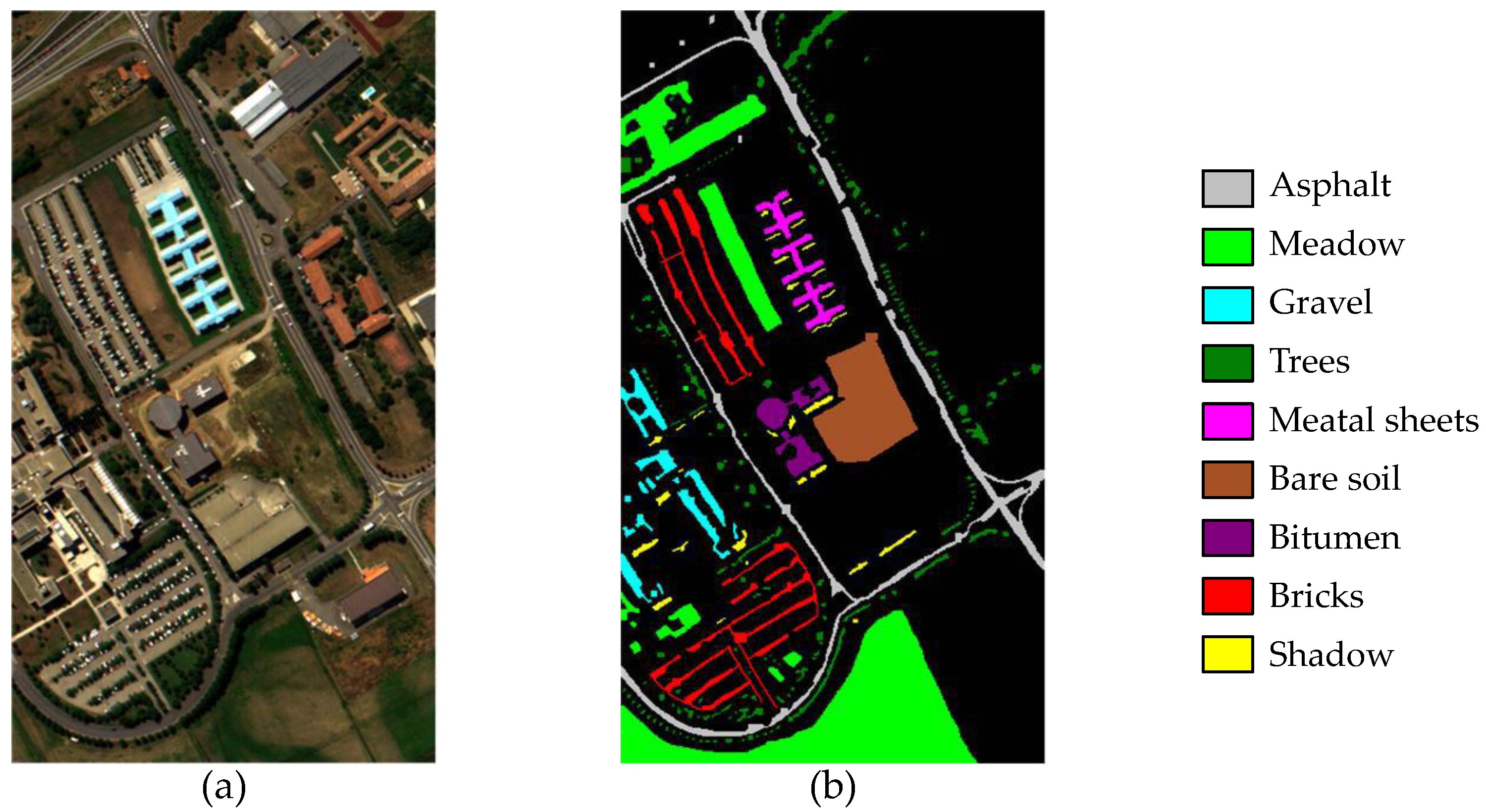
The second dataset is called the Pavia University dataset. It is an urban site over the University of Pavia, Italy. The dataset was captured by the reflective optics system imaging spectrometer (ROSIS-3). The size of the image is 610 × 340 with 1.3 m spatial resolution. The image has 103 spectral bands prior to water-band removal. It has a spectral coverage of 0.43–0.86 μm. A false composite image (R-G-B = band 10-27-46) and the corresponding ground truth are shown in Figure 5a,b. The number of training and testing samples is summarized in Table 2.
The third dataset is the Baffin Bay dataset. It was acquired on 12 April in 2014, from the Hyperion sensor of EO-1. The Hyperion sensor collects 220 spectral bands ranging from 0.4 to 2.5 μm. The sensor operates in a push broom fashion, with a spatial resolution of 30 m for all bands. There are mainly four classes from the ground truth map: Land, sea water, gray ice and white ice. A false composite image and the corresponding ground truth are shown in Figure 6a,b. The number of training and testing samples is listed in Table 3. It should be noted that this dataset is very challenging for hyperspectral image classification. There are many small pieces of white ice in the dataset, and it is very hard to classify these white ice pieces correctly.
4.2. Analysis of Parameters
In the Random Multi-Graphs algorithm [38], the authors have provided a detailed analysis of and . They have demonstrated that the influence of and is limited. In Zhang’s work [38], is set as 0.1, and is set to a fixed small value, . We use the same and values in the proposed SS-RMG. Here, we mainly focus on the discussion about the particular parameters used in the proposed SS-RMG: The number of graphs, the number of spectral bands, and the patch size in LBP feature extraction. In this subsection, OA is selected as the metric. All the results are obtained by averaging the accuracy results of 30 runs.
In the proposed SS-RMG, the number of graphs is an important parameter. We present the experiments about the effect of . Figure 7 illustrates the influence of graph numbers on three datasets. We can see that there is an increase when . When is above 20, the OA values on three datasets tend to be stable. Although utilizing more graphs may contribute to a better result, the improvement is slight. Therefore, we may draw the conclusion that is an available setting, since continuously increasing the number of graphs contributes little to the improvement of accuracy.
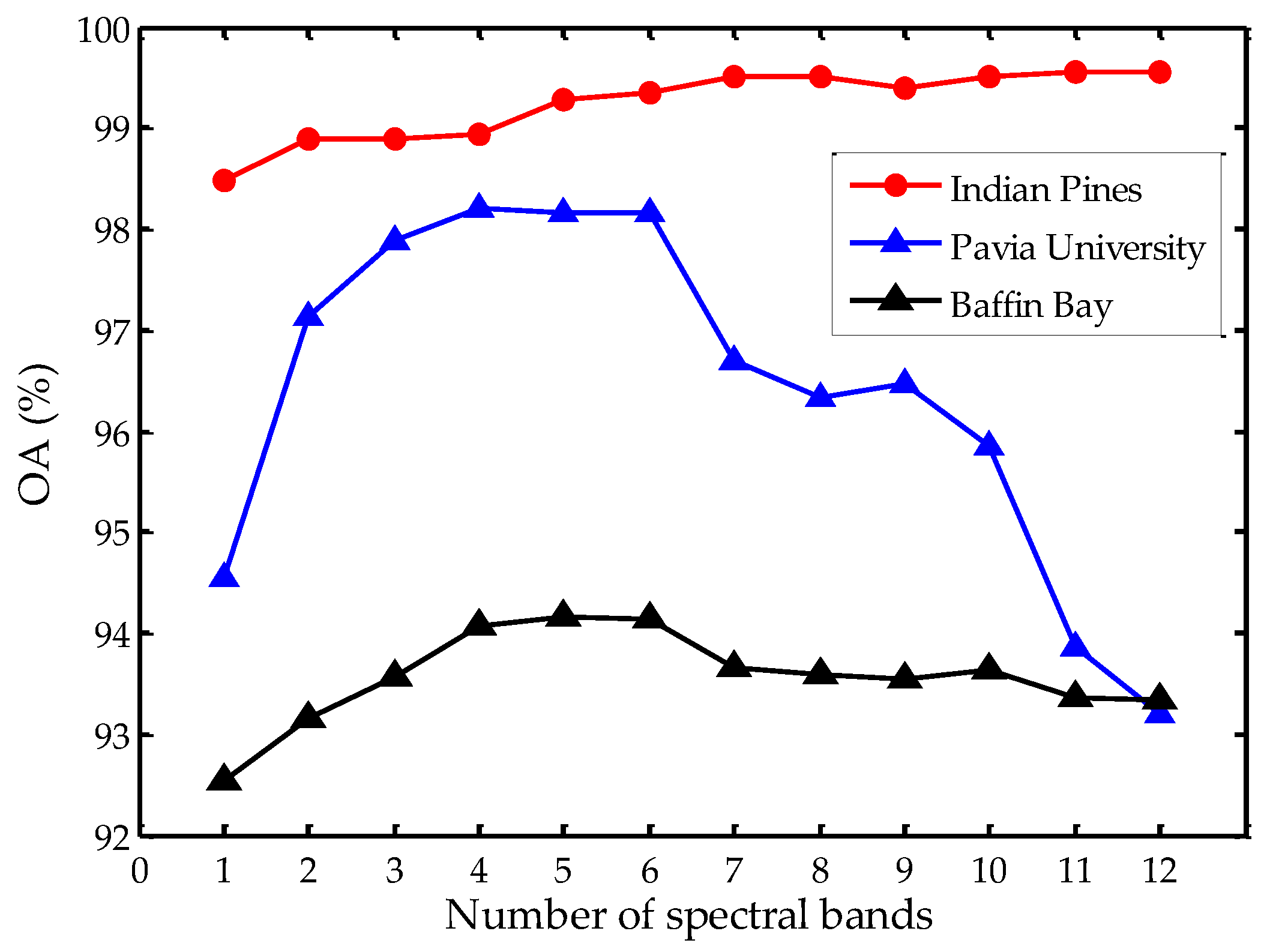
The number of bands used in the proposed SS-RMG also affects the final classification results. Here, we set the number of bands from 1 to 12 to analyze the influence on the three datasets, as illustrated in Figure 8. It can be observed that after an increase from 1 to 7, the value of OA on the Indian Pines dataset presents a steady tendency. However, on the Pavia University dataset, there is a sharp decline when the number of bands is above 5. Similarly, on the Baffin Bay dataset, there is a slow decline when the number of bands is above 6. In our implementations, we set the number of bands as 5. Using 5 spectral bands in the proposed SS-RMG may not be the best choice for all the experimental datasets. Here, we choose a relatively small number, within allowable hardware resources, for better analysis. On the Indian Pines dataset, the spatial and spectral feature vector dimension is 495. 295 elements correspond to spatial features and 200 elements correspond to spectral features. On the Pavia University dataset, the spatial and spectral feature vector dimension is 398. 295 elements correspond to spatial features and 103 elements correspond to spectral features. On the Baffin Bay dataset, the spatial and spectral feature vector dimension is 515. 295 elements correspond to spatial features and 220 elements correspond to spectral features.
Besides the number of graphs and the number of spectral bands, the patch size w in LBP feature extraction is also an important parameter. We set w to 7, 11, 15, 19, 23, 27, 31, 35, 39 and 43 to analyze the influence on the three datasets, as illustrated in Figure 9. We notice that there is a sharp increase in classification accuracy when w ranges from 7 to 19. The accuracy tends to be stable when w is 19 or larger on the Indian Pines dataset. On the Pavia University and Baffin Bay datasets, the classification accuracies decline slightly when w ranges from 19 to 43. A larger patch size would take pixels of different classes into account, and therefore have negative effects in classification accuracy. If the patch size is too small, the extracted features may not be representative for the center pixel’s spatial characteristics. Hence, in our experiments, we set the patch size in LBP feature extraction to 19 × 19 pixels.
4.3. Classification Results
The performance of the proposed SS-RMG is shown in Table 4, Table 5 and Table 6 for the three datasets with different methods. We compare the proposed method with some closely related hyperspectral classification methods: EPF-G [54], IFRF [55], LBP-ELM [39], and R-VCANet [26]. EPF-G generates pixel-wise classification maps, and handles these maps by edge-preserving filtering. Then, the class of each pixel is selected based on the maximum probability. IFRF combines spatial and spectral information via image fusion and recursive filtering. IFRF does not directly extract patches’ features, and it uses two parameters and to extract spatial features. In LBP-ELM, LBP is implemented to represent the spectral and texture features, and a soft-decision fusion process of extreme learning machines was used to merge the probability outputs of spectral and texture features. R-VCANet is a simplified deep learning model. It is comprised of the input layer, two convolutional layers, and the output layer. In the input layer, a rolling guidance filter is used to explore the contextual structure features and remove small details.
We run the above methods 30 times with randomly selected training and testing samples, and the average accuracies and the corresponding standard deviations are reported. Overall accuracy (OA) and kappa coefficient (K) are selected as criterions to give quantitative evaluations.
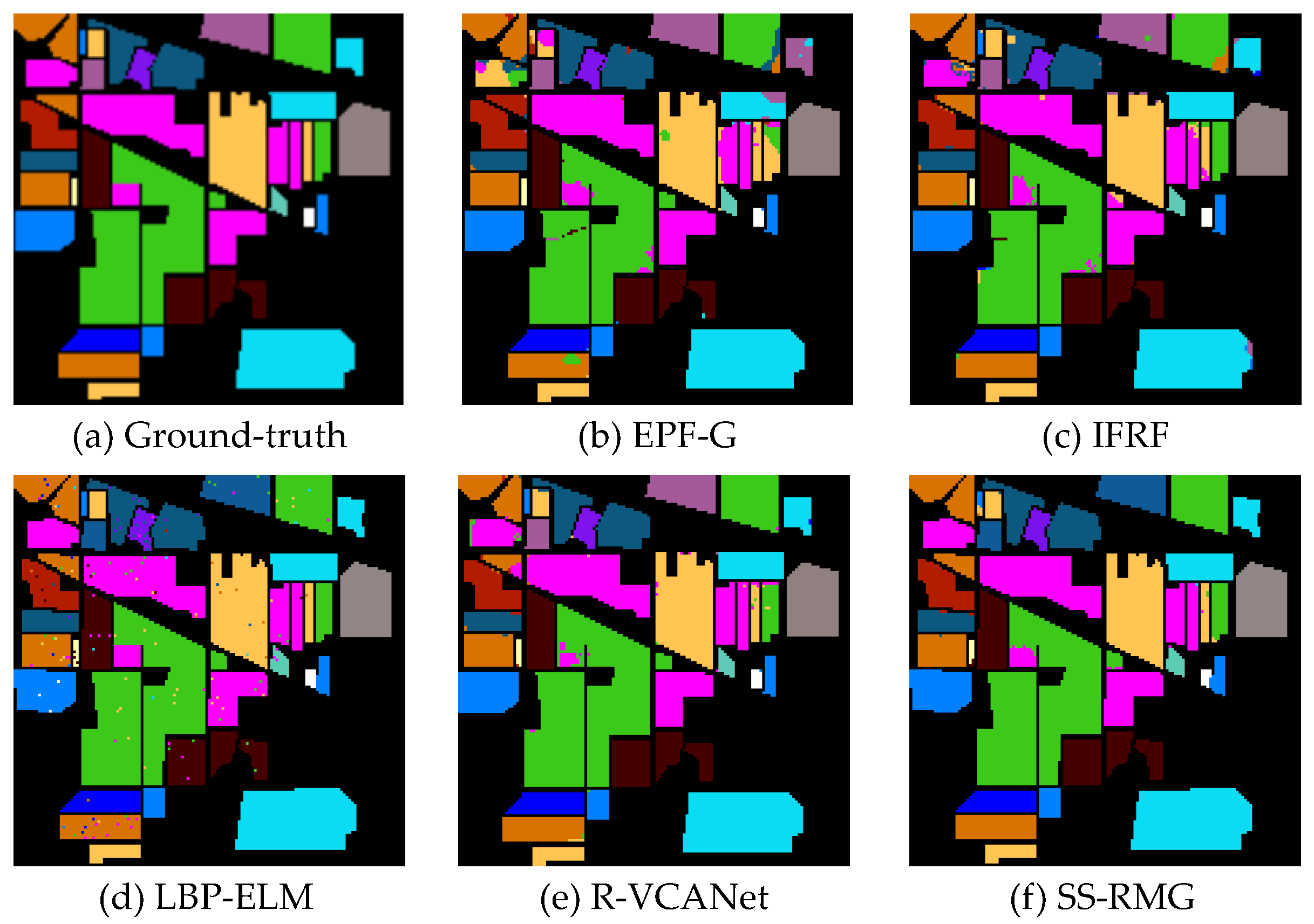
(1) Results on the Indian Pines dataset: In this dataset, 10% of the pixels are selected as the training set and the rest of the pixels in the image are selected for testing. Experimental results on this dataset show that nearly all the methods work. We can observe from Figure 10 that the spatial consistency is roughly preserved by all these methods. The reason for this phenomenon is that these methods have utilized joint spatial–spectral features. The proposed SS-RMG achieves a 1–7% advantage over the other methods. The experimental results on this dataset demonstrate that the Random Multi-Graphs algorithm is effective in hyperspectral image classification, especially when the number of training samples is limited.
(2) Results on the Pavia University dataset: In this dataset, 1% of the pixels are selected as the training set and the rest of the pixels in the image are selected for testing. All the methods show close results. The proposed SS-RMG surpasses LBP-ELM by 6% in OA. It is evident that the proposed SS-RMG outperforms LBP-ELM by randomly selecting subsets of features. In addition, the proposed SS-RMG outperforms EPF-G and IFRF, which means that the application of LBP features can improve the classification performance. Moreover, the proposed SS-RMG surpasses R-VCANet by 1.4% of OA. This result indicates that ensemble learning models can achieve competitive performance compared with deep learning methods in hyperspectral image classification. The results on this dataset indicate that compared with some state-of-the-art methods, the proposed method is predominant. The randomness in the proposed SS-RMG can be viewed as a kind of regularization technique, and it may alleviate the phenomenon of over fitting.
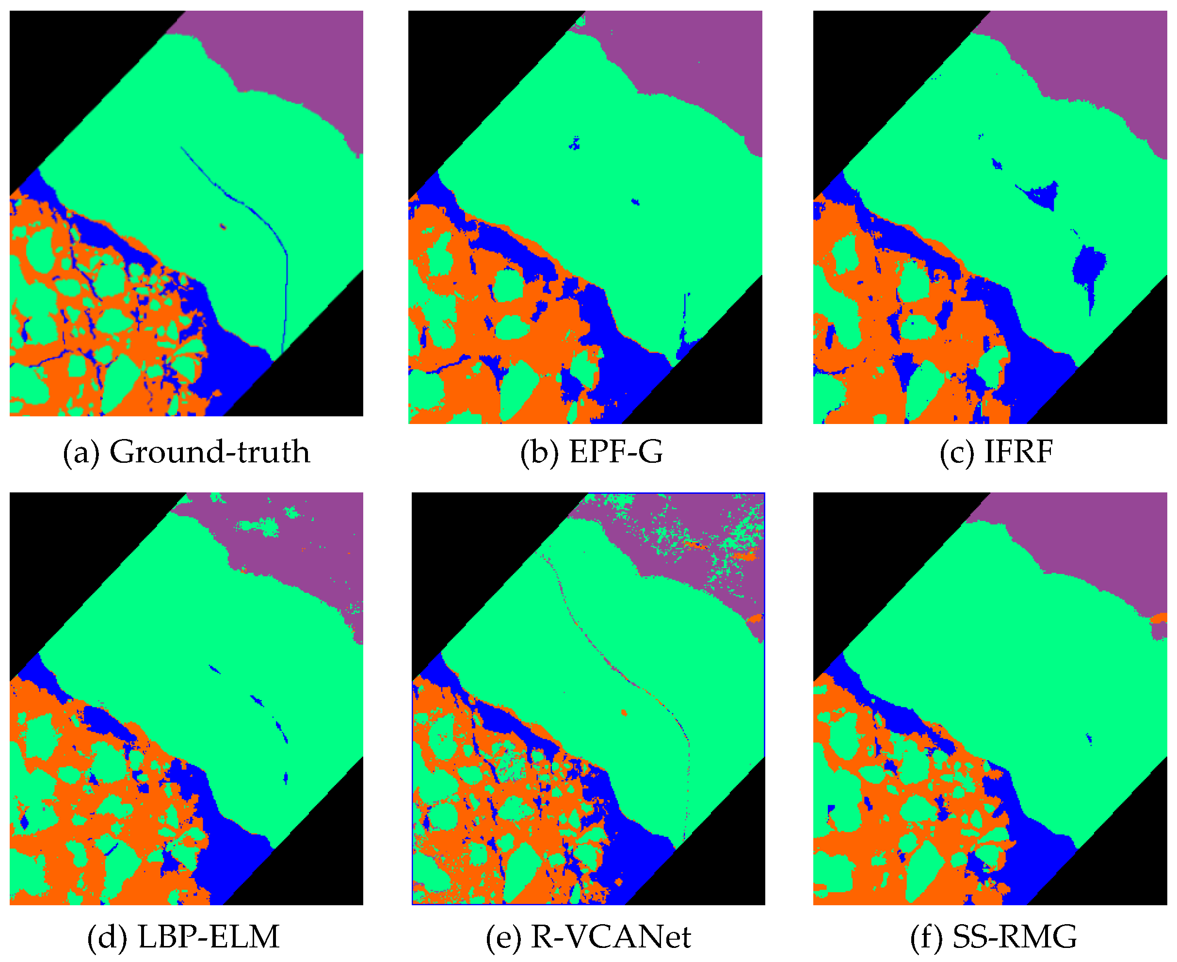
(3) Results on the Baffin Bay dataset: As mentioned before, previous studies mainly focus on ground cover classification, and a sea ice dataset is rarely considered. The Baffin Bay dataset covers a region between the Baffin Island and the southwest coast of Greenland. In this dataset, 1% of the pixels are selected as the training set and the rest of the pixels in the image are selected for testing. From Figure 11, we can observe that in the results generated by EPF-G and IFRF, a lot of small white ice is classified incorrectly into gray ice. Therefore, the classification accuracies of EPF-G and IFRF are lower than the proposed method. From Table 6, we can observe that the proposed SS-RMG surpasses LBP-ELM by 2.2% in OA. Furthermore, in comparison with R-VCANet, the proposed method obtains a 1.5% improvement in OA. This indicates that the proposed SS-RMG is effective in feature extraction and classification. The experimental results on this dataset indicate that the proposed method can achieve good accuracy in sea ice classification by capturing the intrinsic inter-class discriminative patterns.
4.4. Analysis and Discussion
Figure 10, Figure 11 and Figure 12 illustrates the classification results on the three datasets. The classification maps generated by the proposed SS-RMG are obviously less noisy than the other methods, e.g., the regions of Land in Figure 11. The visual results are consistent with those in Table 4, Table 5 and Table 6.
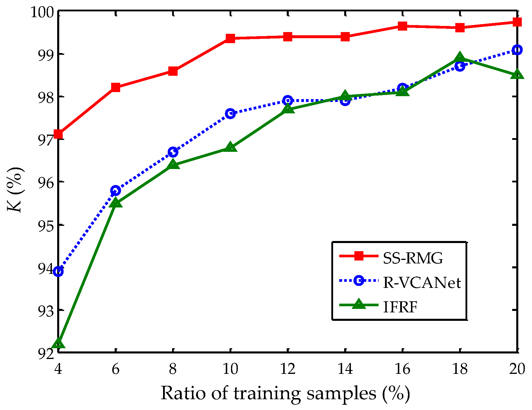
The number of training samples is an important concern in hyperspectral image classification, since the number of training samples is often limited. In some studies, 50% of all the labeled pixels are selected as training samples [18,27]. Figure 13 shows the influences of training samples on the Indian Pines dataset. The number of training samples is large enough to depict the tendency. SS-RMG, R-VCANet, and IFRF present the best classification results among all the methods, therefore they are displayed in Figure 13. These results are obtained by averaging the accuracy results of 30 runs. When the ratio of training samples is above 10%, the classification accuracies of SS-RMG tend to be stable. Therefore, we draw the conclusion that 10% is enough to learn a representative model for this dataset. Moreover, it can be observed from Figure 13 that, compared with R-VCANet and IFRF, the proposed SS-RMG can achieve good classification results with less training samples.
Some recently proposed deep learning models, such as pixel-pair features learned by deep convolutional neural networks (CNN-PPF) [23], have attracted considerable attention. CNN-PPF is a CNN-based classification method based on deep pixel-pair features. The pixel-pair model is used to exploit the similarity between pixels and ensure a sufficient amount of input data to learn a large number of parameters in the CNN. The model is comprised of ten convolutional layers and three max-pooling layers. In the implementations of CNN-PPF, 200 labeled pixels per class are needed for training, and the other pixels are used for testing. To compare the classification performance between CNN-PPF and the proposed SS-RMG, we use the same number of training and testing samples as mentioned in [23].
Table 7 lists the class-specific accuracy and OA for the Indian Pines dataset. It should be noted that the classification result of CNN-PPF is directly obtained from Li’s work [23], and the result of SS-RMG is obtained by the average value of running 30 times. We can observe that the proposed SS-RMG is superior to CNN-PPF, and yields over 3% higher accuracy. Particularly for Soybean-mintill, the class-specific accuracy of the proposed SS-RMG is about 10.4% higher than CNN-PPF. The comparison with CNN-PPF demonstrates that graph-based ensemble learning methods can obtain competitive classification results. Sometimes, the graph-based ensemble model can even generate better classification results.
The computational complexity of the proposed method and other closely related methods is reported in Table 8. All experiments were implemented on the Intel Xeon E5-1620 platform. The computational cost of the proposed SS-RMG is higher than EPF-G, IFRF, and LBP-ELM, due to the fact that SS-RMG carries the burden of graph construction. It is worth noting that the graph constructions are performed independently, which means that this procedure can potentially be performed in parallel. Thus, the speed of the proposed SS-RMG can be further improved. Moreover, compared with R-VCANet, the proposed SS-RMG is superior, which means that the speed of SS-RMG is quite competitive to some deep learning models.
Overall, the experimental results on two popular datasets and one sea ice dataset could imply that the proposed SS-RMG is an effective graph-based ensemble learning model for hyperspectral image classification. It can capture the intrinsic inter-class discriminative patterns, and only limited training samples are needed.
5. Conclusions and Future Work
In this paper, we propose a spectral and spatial classification framework based on Random Multi-Graphs for hyperspectral image classification. First, spatial features are extracted based on LBP. Then, spatial and spectral features are stacked into high dimensional vectors. Second, the high dimensional vectors are fed into Random Multi-Graphs for classification. By randomly selecting a subset of features to create a graph, the proposed method can achieve satisfying classification performance. Compared with closely related methods, the proposed method exhibits good performance. It can be concluded that the proposed method can handle the hyperspectral classification task with limited training samples.
Internal variability has enhanced the greenhouse gas forced Arctic sea ice decline in the past decades [56]. The observed decline in Arctic sea ice opens shorter trade routes across the Arctic Ocean. These routes will allow swifter deliveries between Europe and Asia. Therefore, it is important to monitoring the sea ice along these routes for safe navigation. Hence, in the future, we will focus on developing Arctic sea ice classification methods for hyperspectral images.
Author Contributions
F.G. proposed the original idea and designed the study. F.G. and Q.W. designed and performed the experiments. Q.W., J.D., Q.X. contributed to the discussion of the results. F.G. wrote the manuscript which was revised by all authors.
Funding
This research was funded by the National Natural Science Foundation of China (Grant Nos. 41606198, and 61576011) and in part by the Shandong Provincial Natural Science Foundation under Grant No. ZR2016FB02.
Acknowledgments
The authors would like to thank W. Li, X. Kang and Y. Chen for sharing their code. The authors would also like to thank the Associate Editor and four anonymous reviewers for their very insightful comments and suggestions. These suggestions have greatly improved the quality of this paper.
Conflicts of Interest
The authors declare no conflict of interest.
References
- Horig, B.; Kuhn, F.; Oschutz, F.; Lehmann, F. HyMap hyperspectral remote sensing to detect hydrocarbons. Int. J. Remote Sens. 2010, 4, 1413–1422. [Google Scholar] [CrossRef]
- Butz, C.; Grosjean, M.; Fischer, D.; Wunderle, S.; Tylmann, W.; Rein, B. Hyperspectral imaging spectroscopy: A promising method for the biogeochemical analysis of lake sediments. J. Appl. Remote Sens. 2015, 9, 096031. [Google Scholar] [CrossRef]
- Qin, Q.; Zhang, Z.; Chen, L.; Wang, N.; Zhang, C. Oil and gas reservoir exploration based on hyperspectral remote sensing and super-low-frequency electromagnetic detection. J. Appl. Remote Sens. 2016, 10, 016017. [Google Scholar] [CrossRef]
- Jin, X.; Jie, L.; Wang, S.; Qi, H.; Li, S. Classifying wheat hyperspectral pixels of healthy heads and fusarium head blight disease using a deep neural network in the wild field. Remote Sens. 2018, 10, 395. [Google Scholar] [CrossRef]
- Chen, M.; Wang, Q.; Li, X. Discriminant analysis with graph learning for hyperspectral image classification. Remote Sens. 2018, 10, 836. [Google Scholar] [CrossRef]
- Jia, S.; Hu, J.; Xie, Y.; Shen, L.; Jia, X.; Li, Q. Gabor cube selection based multitask joint sparse representation for hyperspectral image classification. IEEE Trans. Geosci. Remote Sens. 2016, 54, 3174–3187. [Google Scholar] [CrossRef]
- Hughes, G.F. On the mean accuracy of statistical pattern recognizers. IEEE Trans. Inf. Theory 1968, 14, 55–63. [Google Scholar] [CrossRef]
- Gong, M.; Zhang, M.; Yuan, Y. Unsupervised band selection based on evolutionary multiobjective optimization for hyperspectral images. IEEE Trans. Geosci. Remote Sens. 2016, 54, 544–557. [Google Scholar] [CrossRef]
- Chen, Y.; Jiang, H.; Li, C.; Jia, X.; Ghamisi, P. Deep feature extraction and classification of hyperspectral images based on convolutional neural networks. IEEE Trans. Geosci. Remote Sens. 2016, 54, 6232–6251. [Google Scholar] [CrossRef]
- Yuan, Y.; Lin, J.; Wang, Q. Hyperspectral image classification via multi-task joint sparse representation and stepwise MRF optimization. IEEE Trans. Cybern. 2016, 46, 2966–2977. [Google Scholar] [CrossRef] [PubMed]
- Camps-Valls, G.; Tuia, G.; Bruzzone, L. Advances in hyperspectral image classification. IEEE Signal Process. Mag. 2014, 31, 45–54. [Google Scholar] [CrossRef]
- Benediktsson, J.; Palmason, J.; Sveinsson, J. Classification of hyperspectral data from urban areas based on extended morphological profiles. IEEE Trans. Geosci. Remote Sens. 2005, 43, 480–490. [Google Scholar] [CrossRef]
- Li, J.; Bioucas-Dias, J.; Plaza, A. Spectral-spatial hyperspectral image segmentation using subspace mul-timodal logistic regression and Markov random fields. IEEE Trans. Geosci. Remote Sens. 2012, 50, 809–823. [Google Scholar] [CrossRef]
- Tarbalka, Y.; Fauvel, M.; Chanussot, J.; Benediktsson, J.A. SVM and MRF-based method for accurate classification of hyperspectral images. IEEE Geosci. Remote Sens. Lett. 2010, 7, 736–740. [Google Scholar] [CrossRef]
- Wang, Q.; Meng, Z.; Li, X. Locality adaptive discriminant analysis for spectral-spatial classification of hyperspectral images. IEEE Geosci. Remote Sens. Lett. 2017, 14, 2077–2081. [Google Scholar] [CrossRef]
- Makantasis, K.; Doulamis, A.; Doulamis, N.; Nikitakis, A. Tensor-based classification models for hyperspectral data analysis. IEEE Trans. Geosci. Remote Sens. 2018, 56, 1–15. [Google Scholar] [CrossRef]
- Chen, Y.; Lin, Z.; Zhao, X.; Wang, G.; Gu, Y. Deep learning-based classification of hyperspectral data. IEEE J. Sel. Top. Appl. Earth Obs. Remote Sens. 2014, 7, 2094–2107. [Google Scholar] [CrossRef]
- Chen, Y.; Zhao, X.; Jia, X. Spectral-spatial classification of hyperspectral data based on deep belief network. IEEE J. Sel. Top. Appl. Earth Obs. Remote Sens. 2015, 8, 2381–2392. [Google Scholar] [CrossRef]
- Chen, Y.; Zhu, L.; Ghamisi, P.; Jia, X.; Li, G.; Tang, L. Hyperspectral images classification with gabor filtering and convolutional neural network. IEEE Geosci. Remote Sens. Lett. 2017, 14, 2355–2359. [Google Scholar] [CrossRef]
- Chen, Y.; Li, C.; Ghamisi, P.; Jia, X.; Gu, Y. Deep fusion of remote sensing data for accurate classification. IEEE Geosci. Remote Sens. Lett. 2017, 14, 1253–2157. [Google Scholar] [CrossRef]
- Ding, C.; Li, Y.; Xia, Y.; Wei, W.; Zhang, L.; Zhang, Y. Convolutional neural networks based hyperspectral image classification method with adaptive kernels. Remote Sens. 2017, 9, 618. [Google Scholar] [CrossRef]
- Wu, H.; Prasad, S. Convolutional recurrent neural networks for hyperspectral data classification. Remote Sens. 2017, 9, 298. [Google Scholar] [CrossRef]
- Li, W.; Wu, G.; Zhang, F.; Du, Q. Hyperspectral image classification using deep pixel-pair features. IEEE Trans. Geosci. Remote Sens. 2017, 55, 844–853. [Google Scholar] [CrossRef]
- Li, J.; Xi, B.; Li, Y.; Du, Q.; Wang, K. Hyperspectral classification based on texture feature enhancement and deep belief networks. Remote Sens. 2018, 10, 396. [Google Scholar] [CrossRef]
- Zhong, P.; Gong, Z.; Li, S.; Schonlieb, C.B. Learning to diversify deep belief networks for hyperspectral image classification. IEEE Trans. Geosci. Remote Sens. 2017, 55, 3516–3530. [Google Scholar] [CrossRef]
- Pan, B.; Shi, Z.; Xu, X. R-VCANet: A new deep-learning-based hyperspectral image classification method. IEEE J. Sel. Top. Appl. Earth Obs. Remote Sens. 2017, 10, 1975–1986. [Google Scholar] [CrossRef]
- Pan, B.; Shi, Z.; Zhang, N.; Xie, S. Hyperspectral image classification based on nonlinear spectral-spatial network. IEEE Geosci. Remote Sens. Lett. 2016, 13, 1782–1786. [Google Scholar] [CrossRef]
- Makantasis, K.; Karantzalos, K.; Doulamis, A.; Doulamis, N. Deep supervised learning for hyperspectral data classification through convolutional neural networks. In Proceedings of the IEEE International Geoscience and Remote Sensing Symposium, Milan, Italy, 26–31 May 2015; pp. 4959–4962. [Google Scholar]
- Zhang, M.; Li, W.; Du, Q. Diverse region-based CNN for hyperspectral image classification. IEEE Trans. Image Process. 2018, 27, 2623–2634. [Google Scholar] [CrossRef] [PubMed]
- Xu, X.; Li, W.; Ran, Q.; Gao, L.; Zhang, B. Multisource remote sensing data classification based on convolutional neural network. IEEE Trans. Geosci. Remote Sens. 2018, 56, 937–949. [Google Scholar] [CrossRef]
- Song, X.; Jiao, L.; Yang, S.; Zhang, X.; Shang, F. Sparse coding and classifier ensemble based multi-instance learning for image categorization. Signal Process. 2013, 93, 1–11. [Google Scholar] [CrossRef]
- Santos, A.; Araujo, A.; Menotti, D. Combining multiple classification mehthods for hyperspectral data interpretation. IEEE J. Sel. Top. Appl. Earth Obs. Remote Sens. 2013, 6, 1450–1459. [Google Scholar] [CrossRef]
- Ceamanos, X.; Waske, B.; Benediktsson, J.A.; Chanussot, J.; Fauvel, M.; Sveinsson, J.R. A classifier ensemble based on fusion of support vector machines for classfying hyperspectral data. Int. J. Image Data Fusion 2010, 1, 293–307. [Google Scholar] [CrossRef] [Green Version]
- Huang, X.; Zhang, L. An SVM ensemble approach combining spectral, sturctural, and semantic features for the classification of high-resolution remotely sensed imagery. IEEE Trans. Geosci. Remote Sens. 2013, 51, 257–272. [Google Scholar] [CrossRef]
- Gu, Y.; Liu, H. Sample-screening MKL method via boosting strategy for hyperspectral image classification. Neurocomputing 2016, 173, 1630–1639. [Google Scholar] [CrossRef]
- Qi, C.; Zhou, Z.; Sun, Y.; Song, H.; Hu, L.; Wang, Q. Feature selection and multiple kernel boosting framework based on PSO with mutation mechanism for hyperspectral classification. Neurocomputing 2017, 220, 181–190. [Google Scholar] [CrossRef]
- Zhang, E.; Zhang, X.; Jiao, L.; Li, L.; Hou, B. Spectral-spatial hyperspectral image ensemble classification via joint sparse representation. Pattern Recogit. 2016, 59, 42–54. [Google Scholar] [CrossRef]
- Zhang, Q.; Sun, J.; Zhong, G.; Dong, J. Random multi-graphs: a semi-supervised learning framework for classification of high dimensional data. Image Vis. Comput. 2017, 60, 30–37. [Google Scholar] [CrossRef]
- Li, W.; Chen, C.; Su, H.; Du, Q. Local binary patterns and extreme learning machine for hyperspectral imagery classification. IEEE Trans. Geosci. Remote Sens. 2015, 53, 3681–3693. [Google Scholar] [CrossRef]
- Du, Q.; Yang, H. Similarity-based unsupervised band selection for hyperspectral image analysis. IEEE Geosci. Remote Sens. Lett. 2008, 5, 546–568. [Google Scholar]
- Ojala, T.; Peitikainen, M.; Maenpaa, T. Multiresolution gray-scale and rotation invariant texture classification with local binary pattern. IEEE Trans. Pattern Anal. Mach. Intell. 2002, 24, 971–987. [Google Scholar] [CrossRef]
- Rawat, W.; Wang, Z. Deep convolutional neural networks for image classification: A comprehensive review. Neural Comput. 2017, 29, 2352–2449. [Google Scholar] [CrossRef] [PubMed]
- Tang, P.; Wang, X.; Feng, B.; Liu, W. Learning multi-instance deep discriminative patterns for image classification. IEEE Trans. Image Process. 2017, 26, 3385–3396. [Google Scholar] [CrossRef] [PubMed]
- Xu, P.; Sarikaya, R. Contextual domain classification in spoken language understanding systems using recurrent neural network. In Proceedings of the IEEE International Conference on Acoustics, Speech and Signal Processing (ICASSP), Florence, Italy, 4–9 May 2014; pp. 136–140. [Google Scholar]
- Price, M.; Glass, J.; Chandrakasan, A. A low-power speech recognizer and voice activity detector using deep neural networks. IEEE J. Solid-State Circuits 2018, 53, 66–75. [Google Scholar] [CrossRef]
- Zhu, X.; Tuia, D.; Mou, L.; Xia, G.-S.; Zhang, L.; Xu, F.; Fraundorfer, F. Deep learning in remote sensing: A comprehensive review and list of resources. IEEE Geosci. Remote Sens. Mag. 2017, 5, 8–36. [Google Scholar] [CrossRef]
- Zhang, L.; Zhang, L.; Du, B. Deep learning for remote sensing data: A technical tutorial on the state of the art. IEEE Geosci. Remote Sens. Mag. 2016, 4, 22–40. [Google Scholar] [CrossRef]
- Ghamisi, P.; Plaza, J.; Chen, Y.; Li, J.; Plaza, A. Advanced spectral classifiers for hyperspectral images: A review. IEEE Geosci. Remote Sens. Mag. 2017, 5, 8–32. [Google Scholar] [CrossRef]
- Liu, W.; Wang, J.; Chang, S. Hashing with graphs. In Proceedings of the International Conference on Machine Learning, Bellevue, WA, USA, 28 June–2 July 2011; pp. 1–8. [Google Scholar]
- Kim, S.; Choi, S. Multi-view anchor graph hashing. In Proceedings of the IEEE International Conference on Acoustics, Speech and Signal Processing, Vancouver, BC, Canada, 26–31 May 2013; pp. 3123–3127. [Google Scholar]
- Liu, W.; He, J.; Chang, S.-F. Large graph construction for scalable semi-supervised learning. In Proceedings of the International Conference on Machine Learning, Haifa, Israel, 21–24 June 2010; pp. 1–8. [Google Scholar]
- Vincent, P.; Larochelle, H.; Lajoie, I.; Bengio, Y.; Manzagol, P.-A. Stacked denoising autoencoders: Learning useful representations in a deep network with a local denosing criterion. J. Mach. Learn. Res. 2010, 11, 3371–3408. [Google Scholar]
- Breiman, L. Random forests. Mach. Learn. 2001, 45, 5–32. [Google Scholar] [CrossRef]
- Kang, X.; Li, S.; Benediktsson, J.A. Spectral-spatial hyperspectral image classification with edge-perserving filtering. IEEE Trans. Geosci. Remote Sens. 2014, 52, 2666–2677. [Google Scholar] [CrossRef]
- Kang, X.; Li, S.; Benediktsson, J.A. Feature extraction of hyperspectral images with image fusion and recursive filtering. IEEE Trans. Geosci. Remote Sens. 2014, 52, 3742–3752. [Google Scholar] [CrossRef]
- Kay, J.E.; Holland, M.M.; Jahn, A. Inter-annual to multi-decadal Arctic sea ice extent trends in a warming world. Geophys. Res. Lett. 2011, 38, L15708. [Google Scholar] [CrossRef]
Figure 1.
Flow chart of the proposed SS-RMG method.

Figure 2.
Implementation of LBP feature extraction.
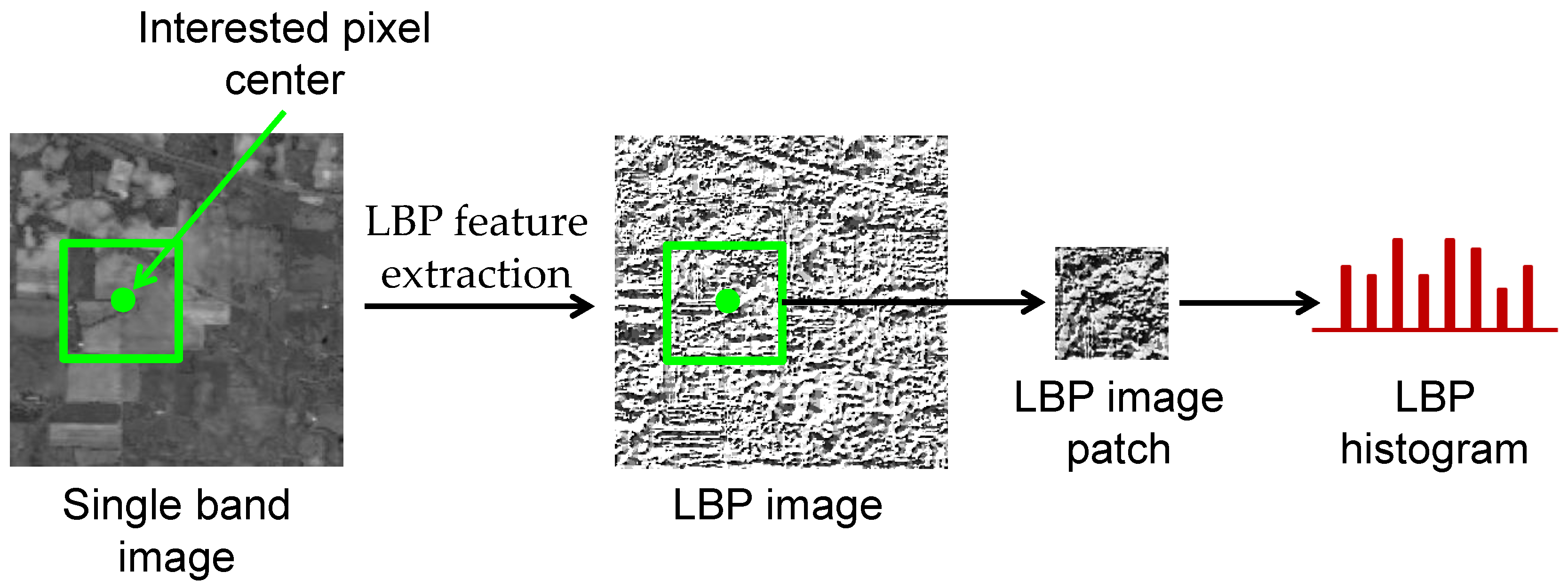
Figure 3.
Flow chart of the Random Multi-Graphs algorithm.

Figure 4.
Indian Pines dataset and corresponding ground truth. (a) False color composite image (R-G-B = band 50-27-17); (b) The ground truth image with 16 land-cover classes.
Figure 4.
Indian Pines dataset and corresponding ground truth. (a) False color composite image (R-G-B = band 50-27-17); (b) The ground truth image with 16 land-cover classes.

Figure 5.
Pavia University dataset and corresponding ground truth. (a) False color composite image (R-G-B = band 10-27-46); (b) The ground truth image with 9 land-cover classes.
Figure 5.
Pavia University dataset and corresponding ground truth. (a) False color composite image (R-G-B = band 10-27-46); (b) The ground truth image with 9 land-cover classes.

Figure 6.
Baffin Bay dataset and corresponding ground truth. (a) False color composite image; (b) The ground truth image with 4 classes.
Figure 6.
Baffin Bay dataset and corresponding ground truth. (a) False color composite image; (b) The ground truth image with 4 classes.
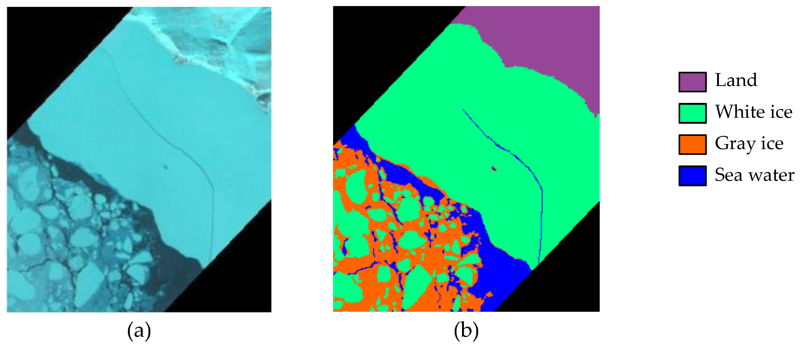
Figure 7.
Influence of graph numbers.
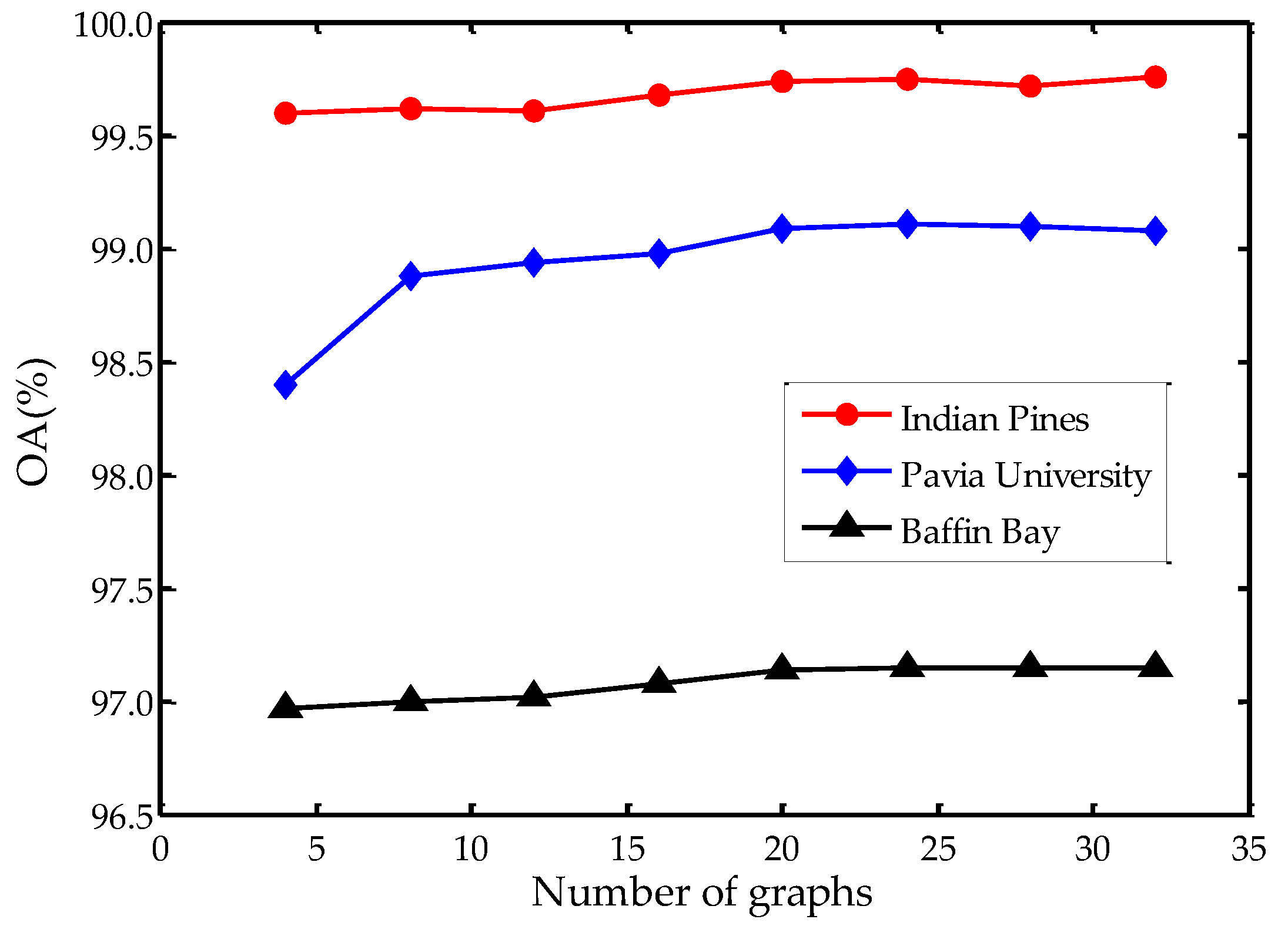
Figure 8.
Influence of spectral band numbers.

Figure 9.
Classification performance versus different patch sizes.
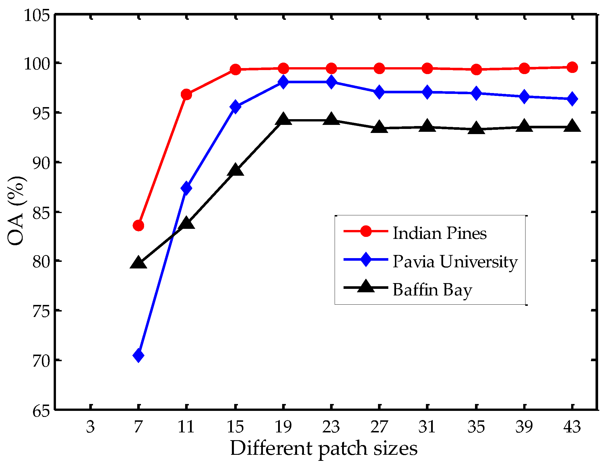
Figure 10.
Classification results by different methods on the Indian Pines dataset. (a) Ground-truth map; (b) EPF-G; (c) IFRF; (d) LBP-ELM; (e) R-VCANet; (f) Proposed SS-RMG.
Figure 10.
Classification results by different methods on the Indian Pines dataset. (a) Ground-truth map; (b) EPF-G; (c) IFRF; (d) LBP-ELM; (e) R-VCANet; (f) Proposed SS-RMG.

Figure 11.
Classification results of different methods on the Baffin Bay dataset. (a) Ground-truth map; (b) EPF-G; (c) IFRF; (d) LBP-ELM; (e) R-VCANet; (f) Proposed SS-RMG.
Figure 11.
Classification results of different methods on the Baffin Bay dataset. (a) Ground-truth map; (b) EPF-G; (c) IFRF; (d) LBP-ELM; (e) R-VCANet; (f) Proposed SS-RMG.

Figure 12.
Classification results of different methods on the Pavia University dataset. (a) Ground-truth map; (b) EPF-G; (c) IFRF; (d) LBP-ELM; (e) R-VCANet; (f) Proposed SS-RMG.
Figure 12.
Classification results of different methods on the Pavia University dataset. (a) Ground-truth map; (b) EPF-G; (c) IFRF; (d) LBP-ELM; (e) R-VCANet; (f) Proposed SS-RMG.
Figure 13.
Influence of training sample number on the Indian Pines dataset.


Table 1.
Train–test distribution of samples for the Indian Pines dataset.
| # | Class | Train | Test |
|---|---|---|---|
| 1 | Alfalfa | 5 | 41 |
| 2 | Corn-notill | 143 | 1285 |
| 3 | Corn-mintill | 83 | 747 |
| 4 | Corn | 24 | 213 |
| 5 | Grass-pasture | 48 | 435 |
| 6 | Grass-trees | 73 | 657 |
| 7 | Grass-pasture-mowed | 3 | 25 |
| 8 | Hay-windrowed | 48 | 430 |
| 9 | Oats | 2 | 18 |
| 10 | Soybean-notill | 97 | 975 |
| 11 | Soybean-mintill | 246 | 2209 |
| 12 | Soybean-clean | 59 | 534 |
| 13 | Wheat | 21 | 184 |
| 14 | Woods | 127 | 1138 |
| 15 | Building-grass-trees-drives | 39 | 347 |
| 16 | Stone-steel-towers | 9 | 84 |
| Total | 1027 | 9322 |
Table 2.
Train–test distribution of samples for the Pavia University dataset.
| # | Class | Train | Test |
|---|---|---|---|
| 1 | Asphalt | 66 | 6565 |
| 2 | Meadows | 186 | 18,463 |
| 3 | Gravel | 21 | 2078 |
| 4 | Trees | 31 | 3033 |
| 5 | Painted metal sheets | 13 | 1332 |
| 6 | Bare Soil | 50 | 4979 |
| 7 | Bitumen | 13 | 1317 |
| 8 | Self-blocking bricks | 37 | 3645 |
| 9 | Shadows | 9 | 938 |
| Total | 426 | 42,350 |
Table 3.
Train-test distribution of samples for the Baffin Bay dataset.
| # | Class | Train | Test |
|---|---|---|---|
| 1 | White ice | 75 | 7429 |
| 2 | Gray ice | 137 | 13,541 |
| 3 | Sea ice | 527 | 52,163 |
| 4 | Land | 114 | 11,281 |
| Total | 853 | 84,414 |
Table 4.
Classification accuracies of different methods on Indian Pines dataset.
| Class | EPF-G | IFRF | R-VCANet | LBP-ELM | SS-RMG |
|---|---|---|---|---|---|
| Alfalfa | 95.85 ± 11.2 | 96.00 ± 2.63 | 98.97 ± 1.65 | 98.53 ± 3.45 | 99.64 ± 0.91 |
| Corn-notill | 93.95 ± 3.08 | 95.29 ± 2.13 | 95.34 ± 1.68 | 97.03 ± 1.08 | 99.48 ± 0.56 |
| Corn-mintill | 96.25 ± 2.95 | 96.03 ± 2.64 | 96.17 ± 1.52 | 96.56 ± 1.99 | 99.93 ± 0.12 |
| Corn | 67.00 ± 9.15 | 94.82 ± 3.75 | 97.38 ± 2.87 | 96.89 ± 4.08 | 98.41 ± 1.24 |
| Grass-pasture | 98.17 ± 1.25 | 97.77 ± 2.90 | 97.80 ± 1.65 | 98.33 ± 2.34 | 99.32 ± 0.80 |
| Grass-trees | 97.97 ± 1.12 | 98.78 ± 0.58 | 99.83 ± 0.17 | 98.07 ± 0.83 | 99.73 ± 0.26 |
| Grass-pasture-mowed | 100.0 ± 0.00 | 96.18 ± 12.2 | 96.00 ± 5.35 | 93.64 ± 5.17 | 93.10 ± 4.40 |
| Hay-windrowed | 99.99 ± 0.04 | 100.0 ± 0.00 | 99.98 ± 0.05 | 99.50 ± 0.91 | 99.40 ± 0.52 |
| Oats | 99.14 ± 3.41 | 90.52 ± 13.5 | 96.29 ± 6.41 | 92.80 ± 11.1 | 99.05 ± 2.38 |
| Soybean-notill | 80.85 ± 4.36 | 94.97 ± 1.85 | 96.13 ± 1.49 | 97.27 ± 0.61 | 98.91 ± 0.46 |
| Soybean-mintill | 95.32 ± 2.08 | 98.11 ± 1.27 | 98.71 ± 0.76 | 98.91 ± 0.41 | 99.53 ± 0.56 |
| Soybean-clean | 87.23 ± 6.66 | 96.79 ± 2.02 | 96.90 ± 1.74 | 98.31 ± 1.64 | 99.41 ± 0.65 |
| Wheat | 100.0 ± 0.00 | 96.90 ± 2.42 | 99.58 ± 0.42 | 99.01 ± 1.83 | 100.0 ± 0.00 |
| Woods | 99.25 ± 0.92 | 99.90 ± 0.32 | 99.83 ± 0.14 | 99.40 ± 0.72 | 99.97 ± 0.04 |
| Building-grass-trees-drives | 78.80 ± 6.70 | 94.90 ± 3.27 | 98.58 ± 1.20 | 99.52 ± 0.65 | 100.0 ± 0.00 |
| Stone-steel-towers | 87.36 ± 5.49 | 95.82 ± 5.74 | 99.08 ± 1.11 | 92.53 ± 9.34 | 98.53 ± 1.03 |
| OA (%) | 92.43 ± 1.18 | 97.21 ± 0.44 | 97.90 ± 0.32 | 98.15 ± 0.33 | 99.44 ± 0.28 |
| K × 100 | 91.33 ± 1.35 | 96.78 ± 0.51 | 97.60 ± 0.37 | 97.89 ± 0.38 | 99.36 ± 0.32 |
Table 5.
Classification accuracies of different methods on Pavia University dataset.
| Class | EPF-G | IFRF | R-VCANet | LBP-ELM | SS-RMG |
|---|---|---|---|---|---|
| Asphalt | 97.35 ± 1.94 | 91.47 ± 3.27 | 94.73 ± 1.78 | 88.15 ± 1.54 | 96.18 ± 0.74 |
| Meadows | 98.54 ± 0.77 | 98.98 ± 0.45 | 99.71 ± 0.19 | 96.08 ± 2.72 | 98.94 ± 0.59 |
| Gravel | 93.19 ± 6.24 | 87.18 ± 4.81 | 89.33 ± 5.25 | 93.43 ± 4.04 | 99.14 ± 0.51 |
| Trees | 87.48 ± 10.1 | 88.81 ± 8.17 | 90.38 ± 3.04 | 76.43 ± 11.2 | 95.46 ± 3.95 |
| Painted metal sheets | 96.77 ± 3.27 | 99.73 ± 0.43 | 99.89 ± 0.15 | 88.69 ± 3.17 | 99.84 ± 0.04 |
| Bare soil | 83.85 ± 8.33 | 94.68 ± 4.09 | 96.81 ± 2.21 | 97.85 ± 1.80 | 99.73 ± 0.16 |
| Bitumen | 88.23 ± 9.07 | 90.19 ± 3.67 | 93.68 ± 3.41 | 95.37 ± 3.20 | 97.05 ± 1.91 |
| Self-blocking bricks | 91.01 ± 3.53 | 85.19 ± 4.82 | 95.09 ± 1.79 | 89.88 ± 3.53 | 96.70 ± 0.72 |
| Shadows | 99.06 ± 0.86 | 77.24 ± 10.5 | 97.06 ± 2.47 | 69.29 ± 10.9 | 99.39 ± 0.27 |
| OA (%) | 93.86 ± 1.76 | 93.73 ± 1.46 | 96.77 ± 0.91 | 92.30 ± 1.05 | 98.14 ± 0.21 |
| K × 100 | 91.86 ± 2.25 | 91.74 ± 1.89 | 95.71 ± 1.21 | 89.73 ± 1.47 | 97.54 ± 0.28 |
Table 6.
Classification accuracies of different methods on Baffin Bay dataset.
| Class | EPF-G | IFRF | R-VCANet | LBP-ELM | SS-RMG |
|---|---|---|---|---|---|
| White ice | 76.00 ± 4.35 | 75.05 ± 7.75 | 85.99 ± 1.13 | 88.38 ± 2.67 | 85.82 ± 1.22 |
| Gray ice | 75.86 ± 2.97 | 72.76 ± 5.20 | 86.85 ± 0.78 | 79.35 ± 0.52 | 82.81 ± 1.90 |
| Sea water | 98.26 ± 0.23 | 98.24 ± 0.68 | 95.14 ± 0.51 | 94.27 ± 1.65 | 97.24 ± 0.52 |
| Land | 99.38 ± 0.52 | 98.00 ± 1.65 | 92.87 ± 1.74 | 99.16 ± 0.29 | 99.43 ± 0.41 |
| OA (%) | 91.94 ± 0.51 | 90.84 ± 1.15 | 92.67 ± 0.34 | 91.90 ± 0.88 | 94.17 ± 0.22 |
| K × 100 | 87.01 ± 1.19 | 84.48 ± 1.78 | 88.09 ± 1.21 | 85.49 ± 1.74 | 90.61 ± 1.11 |
Table 7.
Classification accuracies of CNN-PPF and the proposed SS-RMG on the Indian Pines dataset.
| Class | Training | Testing | CNN-PPF | SS-RMG |
|---|---|---|---|---|
| Corn-notill | 200 | 1228 | 92.99 | 95.63 |
| Corn-mintill | 200 | 630 | 96.66 | 95.64 |
| Grass-pasture | 200 | 283 | 98.58 | 99.88 |
| Grass-trees | 200 | 530 | 100.0 | 100.0 |
| Hay-windrowed | 200 | 278 | 100.0 | 99.83 |
| Soybean-notill | 200 | 772 | 96.24 | 93.18 |
| Soybean-mintill | 200 | 2255 | 87.80 | 98.23 |
| Soybean-clean | 200 | 393 | 98.98 | 97.64 |
| Woods | 200 | 1065 | 99.81 | 99.91 |
| OA | 94.34 | 97.54 |
Table 8.
Computing time of different methods on three datasets (in seconds).
| Dataset | EPF-G | IFRF | R-VCANet | LBP-ELM | SS-RMG |
|---|---|---|---|---|---|
| Indian Pines | 7.31 | 2.37 | 1369.43 | 26.79 | 59.98 |
| Pavia University | 19.72 | 15.96 | 2778.13 | 80.93 | 290.31 |
| Baffin Bay | 26.52 | 20.34 | 4057.32 | 139.20 | 397.47 |
© 2018 by the authors. Licensee MDPI, Basel, Switzerland. This article is an open access article distributed under the terms and conditions of the Creative Commons Attribution (CC BY) license (http://creativecommons.org/licenses/by/4.0/).
Share and Cite
MDPI and ACS Style
Gao, F.; Wang, Q.; Dong, J.; Xu, Q. Spectral and Spatial Classification of Hyperspectral Images Based on Random Multi-Graphs. Remote Sens. 2018, 10, 1271. https://doi.org/10.3390/rs10081271
AMA Style
Gao F, Wang Q, Dong J, Xu Q. Spectral and Spatial Classification of Hyperspectral Images Based on Random Multi-Graphs. Remote Sensing. 2018; 10(8):1271. https://doi.org/10.3390/rs10081271
Chicago/Turabian StyleGao, Feng, Qun Wang, Junyu Dong, and Qizhi Xu. 2018. "Spectral and Spatial Classification of Hyperspectral Images Based on Random Multi-Graphs" Remote Sensing 10, no. 8: 1271. https://doi.org/10.3390/rs10081271
Note that from the first issue of 2016, this journal uses article numbers instead of page numbers. See further details here.