Hyperspectral Image Super-Resolution Inspired by Deep Laplacian Pyramid Network

Abstract

Existing hyperspectral sensors usually produce high-spectral-resolution but low-spatial-resolution images, and super-resolution has yielded impressive results in improving the resolution of the hyperspectral images (HSIs). However, most of the super-resolution methods require multiple observations of the same scene and improve the spatial resolution without fully considering the spectral information. In this paper, we propose an HSI super-resolution method inspired by the deep Laplacian pyramid network (LPN). First, the spatial resolution is enhanced by an LPN, which can exploit the knowledge from natural images without using any auxiliary observations. The LPN progressively reconstructs the high-spatial-resolution images in a coarse-to-fine fashion by using multiple pyramid levels. Second, spectral characteristics between the low- and high-resolution HSIs are studied by the non-negative dictionary learning (NDL), which is proposed to learn the common dictionary with non-negative constraints. The super-resolution results can finally be obtained by multiplying the learned dictionary and its corresponding sparse codes. Experimental results on three hyperspectral datasets demonstrate the feasibility of the proposed method in enhancing the spatial resolution of the HSI with preserving the spectral information simultaneously.

1. Introduction

Hyperspectral imaging systems sample the electromagnetic spectrum of scene radiance by hundreds of contiguous spectral bands. The obtained hyperspectral image (HSI) [1,2,3,4], which has a high spectral resolution, is a data cube containing very narrow spectral bands ranging from the visible to infrared spectrum, enabling the fine representation of different land-covers by spectral signatures. Therefore, HSIs have recently been successfully applied in various tasks, such as classification [5,6,7], unmixing [8,9,10], de-noising [11,12] and detection [13,14,15]. However, the high spectral resolution also comes at a cost, i.e., low-spatial-resolution, that is, the acquired real HSI data usually provides coarse spatial information, and thus are incapable of capturing the details of different objects. Even worse, the low-spatial-resolution will seriously deteriorate the effectiveness of the HSI in applications. This emphasizes the importance of resolution enhancement [16,17].

In addition to developing high-resolution sensors, a natural solution is to perform hyperspectral super-resolution from the algorithmic perspective (It is important to note that not all of the hyperspectral data require one to increase the spatial resolution from the algorithmic perspective. Many HSIs (e.g., high-resolution unmanned aerial vehicles (UAV)-based hyperspectral data), which have very high spatial and spectral resolution, are not needed to increase spatial resolution and thus are not within the scope of this paper.). Existing methods can be roughly divided into three categories. The first category is to fuse an HSI with auxiliary data sources containing high spatial resolution but low-spectral-resolution images of the target scene. Widely used auxiliary observations are the panchromatic (PAN) image and multispectral image (MSI) [18,19]. Many statistics-based fusion methods have been proposed in the literature. For instance, various Bayesian estimators have been designed by formulating the fusion of HSI and PAN/MSI within the Bayesian inference framework [20,21]. Matrix factorization-based methods have also played an important role in enhancing the spatial resolution of HSI. For instance, a coupled non-negative matrix factorization (CNMF) [22] has been proposed to alternately unmix both HSI and PAN/MSI into endmember and abundance matrices. A spatial and spectral fusion model based on sparse matrix factorization [23] has been proposed to combine the spectral and spatial information from different sensors. Moreover, sparse representation has gained much popularity in recent years with the rapid development of compressed sensing. For instance, a super-resolution method termed as GSOMP+ [24] was proposed by generalizing the simultaneous orthogonal matching pursuit with a non-negativity constraint over the solution space. A superpixel-based sparse representation method was developed by [25] to exploit the similarities within superpixels, while hyperspectral super-resolution was achieved by a joint estimation of dictionary and sparse codes in [26]. Although the fusion-based techniques can improve the resolution of the HSIs, they require auxiliary high-spatial-resolution images taken over the same area, which are not always available in practice.

The second category is subpixel mapping (SPM), which divides a mixed pixel into subpixels and assigns class labels to these subpixels. SPM approaches are composed of two major steps, i.e., determining fractional abundances of endmembers in mixed pixels by spectral unmixing or soft classification, and evaluating the subpixel position of each class within a pixel by taking spatial dependence into consideration. Much work has been carried out to enhance the spatial resolution involving the above-mentioned two steps. For instance, a general framework of SPM [27] was proposed to directly incorporate the spectral information into the spatial mapping procedure. Zhang et al. [28] proposed an example-based super-resolution mapping model by using the support vector regression to generate fine resolution maps. An integrated process was performed in [29] to jointly solve the image fusion and spectral unmixing problems. A subpixel resolution thematic map framework is presented in [30], while a collaborative representation-based SPM method [31] was proposed to generate improved classification maps at the subpixel scale. The major limitation of the SPM-based techniques is that they acquire high-spatial-resolution results only for certain applications (e.g., classification).

The third category is single-image super-resolution, which synthesizes image with high spectral and spatial resolutions from the low-spatial-resolution HSI data. A fundamental method for single-image super-resolution is the traditional interpolation, such as bilinear or bicubic interpolation. It is notable that deep learning [32,33,34,35], which can hierarchically learn the high-level abstract representation in deep architectures, has attracted extensive attention due to its impressive results for several different applications. Recently, many super-resolution models based on deep learning have been constructed. For instance, a deep learning-based super-resolution method was proposed in [36] to learn an end-to-end mapping between the low- and high-resolution images. Convolutional neural network (CNN) [37,38] was applied to learn a spectral difference mapping from low-resolution HSI to high-resolution HSI with the spectral information preserved, while Yuan et al. [39] exploited the knowledge from natural images by transferring the learned CNN model to the HSI domain and adopting the CNMF to enforce collaborations between the low- and high-resolution HSIs. A significant benefit of this category is that it does not need the auxiliary PAN or MSI data sources of the same scene.

In this paper, we propose a single-image super-resolution framework inspired by a deep Laplacian pyramid network (LPN) [40,41] to enhance the spatial resolution of the HSIs with the spectral information preserved. As illustrated in Figure 1, the main steps of the proposed method are twofold, i.e., spatial reconstruction by LPN and spectral reconstruction by non-negative dictionary learning (NDL). First, the LPN is trained by using the low- and high-resolution natural image pairs in an end-to-end fashion without stage-wise optimization. Composed of the feature extraction and image reconstruction parts, the LPN can progressively upsample the input low-resolution image to a reconstructed high-resolution image in a coarse-to-fine manner. The trained LPN can be directly utilized to improve the spatial resolution of each spectral band of the HSI. Second, the spectral information is reconstructed by subsequently performing NDL, which is proposed to learn the common dictionary between the original low-resolution HSI and the high-resolution HSI obtained by the LPN. The estimated super-resolution results can be finally generated by multiplying the learned dictionary and its corresponding sparse codes.

To summarize, the main contributions of this work are embodied by the following:

• We present the first attempt, to the best of our knowledge, to introduce the LPN to super-resolution of HSIs. Instead of requiring auxiliary images taken over the same area of the target HSI, the LPN learns an end-to-end mapping from easily acquired natural images. Moreover, the LPN does not need any pre-defined upsampling operators (e.g., bicubic interpolation) to upscale the low-resolution image to the desired size.
• We propose an NDL method for spectral information reconstruction. It is interesting to note that the spectral relation of spectral bands can be conveniently formulated within the dictionary learning framework. Moreover, both sparse codes and the dictionary are constrained to be non-negative, which conforms to physical reality.

The rest of this paper is organized as follows: in Section 2, we give detailed descriptions of the proposed method. In Section 3, experimental results on several benchmark datasets are reported to compare with other methods. Conclusions are drawn in Section 4.

2. Proposed Method

In this section, we provide detailed descriptions of the proposed method, whose main steps are spatial reconstruction by the LPN and spectral reconstruction by NDL.

2.1. Spatial Reconstruction by Deep Laplacian Pyramid Network

Letting ${\mathit{X}}_l$ be the low-resolution image, the general architecture of the LPN is shown in Figure 2, which shows that the LPN model for spatial reconstruction consists of two parts, i.e., feature extraction and image reconstruction.

As illustrated in Figure 2, the feature extraction part contains multiple basic blocks that comprise a feature embedding sub-network, a transposed convolutional layer and a convolutional layer. The feature embedding sub-network applies multiple convolutional layers for transforming the high-dimensional nonlinear feature maps, the transposed convolutional layer can upsample the input features by a scale of 2, and the convolutional layer reconstructs the sub-band residual image. It is worth noting that an additional convolutional layer is added in the first pyramid level to transform the input low-resolution image into high-dimensional nonlinear feature maps, while the feature embedding sub-network in other pyramid levels directly transforms the features from the transposed convolutional layer of the previous level into feature maps. Compared to other networks that realize feature extraction and reconstruction at the finest resolution, the LPN can generate feature maps at the finer resolution with only one transposed convolutional layer.

In the image reconstruction part, the high-resolution image at the level s can be reconstructed by combining the upsampled image with the predicted residual image using element-wise summation. Taking the low-resolution image as input, the residual image can be progressively predicted on the $s={log}_{2}S$ pyramid level, where S refers to the upsampling scale factor and s represents the pyramid level, while the upsampled image is obtained by upsampling the input image using a scale of 2 with a transposed convolutional layer. The high-resolution image at the level s is then taken as the input of the image reconstruction part at level $s+1$, and the entire network is composed of a cascade of feature extraction and image reconstruction sub-networks with the same structure at each level.

Note that the networks at different pyramid levels share the same structure and task, and we can thus share the network parameters of the feature embedding sub-network, transposed convolutional layer, and convolutional layer across all of the levels. In this regard, the parameter number is independent of the upsampling scale factor S and one single set of parameters is required to construct the network with multiple pyramid levels. In addition to sharing parameters across different levels, the parameters can also be shared within each pyramid level. In greater detail, the feature- embedding sub-network can be constructed by a series of recursive blocks. Figure 3 depicts the structure of a recursive block, which consists of D distinct convolutional layers. The rectified linear unit (ReLU) ($R\left(z\right)=max(0,z)$) is a widely used activation function in deep learning. The parameters of those convolutional layers are shared among recursive blocks, and thus the network depth can be effectively increased without increasing the parameter size.

To optimize the parameters $\mathit{\theta }$ in the LPN, we should define an appropriate loss function. The goal of the LPN is to learn a mapping that can generate a high-resolution image ${\widehat{\mathit{X}}}_h$ that is close to the high-resolution ground truth image ${\mathit{X}}_h$. Letting the residual image at level s be ${\widehat{\mathit{R}}}^{\left(s\right)}$, the output high-resolution image ${\widehat{\mathit{X}}}_h^{\left(s\right)}$ at level s can be formulated as ${\widehat{\mathit{X}}}_h^{\left(s\right)}={\mathit{X}}_l^{\left(s\right)}+{\widehat{\mathit{R}}}^{\left(s\right)}$. The ground truth image ${\mathit{X}}_h$ is re-sized to ${\widehat{\mathit{X}}}_h^{\left(s\right)}$ at each level by bicubic downsampling, and the loss function is modeled by

$$\begin{array}{ccc}\mathcal{L}\left(\mathit{\theta }\right)\hfill & =& \frac{1}{I}\sum _{i=1}^I\sum _{s=1}^{{log}_{2}S}\rho \left({\mathit{X}}_h^{(i,s)}-{\widehat{\mathit{X}}}_h^{(i,s)}\right)\hfill \\ & =& \frac{1}{I}\sum _{i=1}^I\sum _{s=1}^{{log}_{2}S}\rho \left(({\mathit{X}}_h^{(i,s)}-{\widehat{\mathit{X}}}_l^{(i,s)})-{\widehat{\mathit{R}}}^{(i,s)}\right),\hfill \end{array}$$

(1)

where I denotes the number of training samples in each batch, $\rho \left(x\right)=\sqrt{x^2+{ϵ}^2}$ represents the Charbonnier penalty function [42], which is strictly convex and infinitely differentiable. Therefore, it is a differentiable variant version of the $l_1$-norm. The convex penalty ensures a unique solution of the optimization problem, and the parameter $ϵ$ determines how closely the penalty function resembles the $l_1$-norm. In this paper, $ϵ$ is set to 1e-3 and the loss function $\mathcal{L}\left(\mathit{\theta }\right)$ is minimized by adopting the stochastic gradient descent (SGD) solver. Having trained the LPN, the spatial resolution of the low-resolution HSI can be determined by taking each spectral band of the HSI as input of the LPN. The high-resolution outputs of the LPN are then stacked into the high-spatial-resolution HSI, whose spectral resolution can be reconstructed by NDL.

2.2. Spectral Reconstruction by Non-Negative Dictionary Learning

Let the matrix ${\mathit{S}}_h\in {\mathbb{R}}^{b\times MN}$ denote the high-spatial-resolution HSI by concatenating the pixels of the HSI ${\mathit{S}}_{h,3D}\in {\mathbb{R}}^{M\times N\times b}$ generated by the LPN, i.e., ${\mathit{S}}_{h,3D}\in {\mathbb{R}}^{M\times N\times b}\to {\mathit{S}}_h\in {\mathbb{R}}^{b\times MN}$, where $M,N$ refer to the spatial dimensions and b represents the number of spectral bands. By assuming that the spectral signatures of pixels belonging to the same class approximately lie in the same low-dimensional subspace [43], the matrix ${\mathit{S}}_h$ can be expressed as

$$\begin{array}{cc}\hfill & {\mathit{S}}_h=\mathit{D}{\mathit{V}}_h,\hfill \\ s.t.\hfill & \left\{\begin{array}{c}\left|\right|{\mathit{V}}_h{\left|\right|}_0\le C_{h0},\hfill \\ {\mathit{d}}_k\ge 0,k=1,2,\dots ,K,\hfill \\ {\mathit{v}}_{hj}\ge 0,j=1,2,\dots ,MN,\hfill \end{array}\right.\hfill \end{array}$$

(2)

where $\mathit{D}=[{\mathit{d}}_1,{\mathit{d}}_2,\dots ,{\mathit{d}}_K]\in {\mathbb{R}}^{b\times K}$ is the dictionary whose columns ${\left\{{\mathit{d}}_k\right\}}_{k=1,2,\dots ,K}$ are the atoms containing the spectral signature of all of the classes, and ${\mathit{V}}_h$ denotes the unknown sparse codes. Both $\mathit{D}$ and ${\mathit{V}}_h$ are constrained to be non-negative, which coincides with the physical reality.

Similarly, the original low-spatial-resolution HSI can also be reshaped as ${\mathit{S}}_l\in {\mathbb{R}}^{b\times mn}$ by concatenating the pixels in the original input HSI ${\mathit{S}}_{l,3D}\in {\mathbb{R}}^{m\times n\times b}$, where $m,n$ denote the spatial dimensions and b is the number of spectral bands. Analogously to ${\mathit{S}}_h$, we can also reformulate ${\mathit{S}}_l$ as

$$\begin{array}{cc}\hfill & {\mathit{S}}_l=\mathit{D}{\mathit{V}}_l,\hfill \\ s.t.\hfill & \left\{\begin{array}{c}\left|\right|{\mathit{V}}_l{\left|\right|}_0\le C_{l0},\hfill \\ {\mathit{d}}_k\ge 0,k=1,2,\dots ,K,\hfill \\ {\mathit{v}}_{lj}\ge 0,j=1,2,\dots ,mn.\hfill \end{array}\right.\hfill \end{array}$$

(3)

Note that both low- and high-resolution HSIs capture the same scene, and the underlying materials of those data are the same. As such, we share the same dictionary $\mathit{D}$ in Equations (2) and (3). In addition, the dictionaries $\mathit{D}$ and ${\mathit{V}}_l$ are constrained to be non-negative to grasp the physical nature of the data. The $l_0$ optimization problems in Equations (2) and (3) can be approximately replaced by $l_1$-based problems. Combining the two $l_1$-based problems, we have

$$\begin{array}{cc}\hfill & arg\underset{\mathit{D},{\mathit{V}}_h,{\mathit{V}}_l}{min}\frac{1}{2}{\left|\left|{\mathit{S}}_l-\mathit{D}{\mathit{V}}_l\right|\right|}_{\mathrm{F}}^2+\frac{\beta }{2}{\left|\left|{\mathit{S}}_h-\mathit{D}{\mathit{V}}_h\right|\right|}_{\mathrm{F}}^2+\lambda {\left|\left|{\mathit{V}}_l\right|\right|}_1+\beta \lambda {\left|\left|{\mathit{V}}_h\right|\right|}_1,\hfill \\ s.t.\hfill & \left\{\begin{array}{c}{\mathit{d}}_k\ge 0,k=1,2,\dots ,K,\hfill \\ {\mathit{v}}_{hj}\ge 0,j=1,2,\dots ,MN,\hfill \\ {\mathit{v}}_{lj}\ge 0,j=1,2,\dots ,mn,\hfill \end{array}\right.\hfill \end{array}$$

(4)

where $\lambda ,\beta$ $(\lambda \ge 0,\beta \ge 0)$ are the regularization parameters.

Letting $\mathit{S}=[{\mathit{S}}_l,\beta {\mathit{S}}_h]$ and $\mathit{V}=[{\mathit{V}}_l,\beta {\mathit{V}}_h]$ , Equation (4) yields

$$\begin{array}{cc}\hfill & arg\underset{\mathit{D},\mathit{V}}{min}\frac{1}{2}{\left|\left|\mathit{S}-\mathit{D}\mathit{V}\right|\right|}_{\mathrm{F}}^2+\lambda {\left|\left|\mathit{V}\right|\right|}_1,\hfill \\ s.t.\hfill & \left\{\begin{array}{c}{\mathit{d}}_k\ge 0,k=1,2,\dots ,K,\hfill \\ {\mathit{v}}_j\ge 0,j=1,2,\dots ,MN+mn.\hfill \end{array}\right.\hfill \end{array}$$

(5)

Up until now, the spectral reconstruction problem has been transformed to a dictionary learning problem displayed in Equation (5), which can be solved by alternatively optimizing a certain variable with other variables fixed. In greater detail, for a fixed dictionary $\mathit{D}$, the sub-problem with respect to $\mathit{V}$ can be written as

$$\begin{array}{cc}\hfill & arg\underset{\mathit{V}}{min}\frac{1}{2}{\left|\left|\mathit{S}-\mathit{D}\mathit{V}\right|\right|}_{\mathrm{F}}^2+\lambda {\left|\left|\mathit{V}\right|\right|}_1,\hfill \\ s.t.\hfill & \begin{array}{c}{\mathit{v}}_j\ge 0,j=1,2,\dots ,MN+mn.\hfill \end{array}\hfill \end{array}$$

(6)

The above-mentioned problem in Equation (6) can be effectively solved by the alternating direction method of multipliers (ADMM) [44]. Reformulating Equation (6), we have

$$\begin{array}{cc}\hfill & arg\underset{\mathit{V}}{min}\frac{1}{2}\left|\right|\mathit{S}-{\mathit{D}\mathit{W}\left|\right|}_{\mathrm{F}}^2+{\lambda \left|\right|\mathit{V}\left|\right|}_1,\hfill \\ s.t.\hfill & \begin{array}{c}\mathit{V}=\mathit{W},{\mathit{v}}_j\ge 0,j=1,2,\dots ,MN+mn,\hfill \end{array}\hfill \end{array}$$

(7)

whose augmented Lagrangian function yields

$$\begin{array}{ccc}{\mathcal{L}}_{\mu }(\mathit{V},\mathit{W},\mathit{T})\hfill & =& \frac{1}{2}{\left|\left|\mathit{S}-\mathit{D}\mathit{W}\right|\right|}_{\mathrm{F}}^2+\lambda {\left|\left|\mathit{V}\right|\right|}_1+<\mathit{T},\mathit{W}-\mathit{V}>+\mu {\left|\left|\mathit{W}-\mathit{V}\right|\right|}_{\mathrm{F}}^2\hfill \\ & & s.t.\begin{array}{c}{\mathit{v}}_j\ge 0,j=1,2,\dots ,MN+mn\hfill \end{array}\hfill \\ & =& \frac{1}{2}{\left|\left|\mathit{S}-\mathit{D}\mathit{W}\right|\right|}_{\mathrm{F}}^2+\lambda {\left|\left|\mathit{V}\right|\right|}_1+\mu {\left|\left|\mathit{W}-\mathit{V}+\frac{\mathit{T}}{2\mu }\right|\right|}_{\mathrm{F}}^2\hfill \\ & & s.t.\begin{array}{c}{\mathit{v}}_j\ge 0,j=1,2,\dots ,MN+mn,\hfill \end{array}\hfill \end{array}$$

(8)

where $\mu >0$ is the penalty parameter and $\mathit{T}$ denotes the Lagrangian multiplier.

Without loss of generality, the matrices $\mathit{W}$ and $\mathit{V}$ in the $(p+1)$th iteration can be determined, respectively, by

$$\begin{array}{ccc}{\mathit{W}}^{(p+1)}\hfill & =& arg\underset{\mathit{W}}{min}{\mathcal{L}}_{\mu }({\mathit{V}}^{\left(p\right)},\mathit{W},{\mathit{T}}^{\left(p\right)})\hfill \\ & =& {({\mathit{D}}^{\mathrm{T}}\mathit{D}+2\mu \mathit{E})}^{-1}\left[{\mathit{D}}^{\mathrm{T}}\mathit{S}+2\mu \left({\mathit{V}}^{\left(p\right)}-\frac{{\mathit{T}}^{\left(p\right)}}{2\mu }\right)\right]\hfill \end{array}$$

(9)

and

$$\begin{array}{ccc}{\mathit{V}}^{(p+1)}\hfill & =& arg\underset{\mathit{V}}{min}{\mathcal{L}}_{\mu }(\mathit{V},{\mathit{W}}^{(p+1)},{\mathit{T}}^{\left(p\right)}),s.t.\begin{array}{c}{\mathit{v}}_j\ge 0\hfill \end{array}\hfill \\ & =& {\left[{\mathcal{S}}_{\frac{\lambda }{2\mu }}\left({\mathit{W}}^{(p+1)}+\frac{{\mathit{T}}^{\left(p\right)}}{2\mu }\right)\right]}_{+},\hfill \end{array}$$

(10)

where $\mathit{E}$ is the identity matrix, ${[·]}_{+}=max\{·,0\}$ and ${\mathcal{S}}_{\frac{\lambda }{2\mu }}$ is the shrinkage operator given by

$$\begin{array}{ccc}{\mathcal{S}}_{\frac{\lambda }{2\mu }}(·)\hfill & =& \mathrm{sign}(·)max\left(0,|·|-\frac{\lambda }{2\mu }\right).\hfill \end{array}$$

(11)

Based on ${\mathit{W}}^{(p+1)}$ and ${\mathit{V}}^{(p+1)}$, the Lagrangian multiplier ${\mathit{T}}^{(p+1)}$ can be updated by

$$\begin{array}{ccc}{\mathit{T}}^{(p+1)}\hfill & =& {\mathit{T}}^{\left(p\right)}+\mu \left({\mathit{W}}^{(p+1)}-{\mathit{V}}^{(p+1)}\right).\hfill \end{array}$$

(12)

Moreover, we update $\mathit{D}$ by fixing $\mathit{V}$

$$\begin{array}{cc}\hfill & arg\underset{\mathit{D}}{min}{\left|\left|\mathit{S}-\mathit{D}\mathit{V}\right|\right|}_{\mathrm{F}}^2,\hfill \\ s.t.\hfill & \begin{array}{c}{\mathit{d}}_k\ge 0,k=1,2,\dots ,K.\hfill \end{array}\hfill \end{array}$$

(13)

Letting ${\mathit{D}}^{\left(q\right)}$ represent the dictionary learned in the qth iteration, and ${\mathit{d}}_k^{(q+1)}={\mathit{d}}_k^{\left(q\right)}+\Delta {\mathit{d}}_k$, the problem in Equation (13) can be solved by the block coordinate descent method [45], that is, only one column of ${\mathit{D}}^{\left(q\right)}$ is updated in each iteration while keeping other columns fixed, and $\Delta {\mathit{d}}_k$ can be determined by

$$\begin{array}{ccc}\Delta {\mathit{d}}_k\hfill & =& arg\underset{\Delta {\mathit{d}}_k}{min}{\left|\left|\mathit{S}-\left[{\mathit{d}}_1^{\left(q\right)},{\mathit{d}}_2^{\left(q\right)},\dots ,{\mathit{d}}_{k-1}^{\left(q\right)},{\mathit{d}}_k^{\left(q\right)}+\Delta {\mathit{d}}_k,\dots ,{\mathit{d}}_K^{\left(q\right)}\right]\mathit{V}\right|\right|}_{\mathrm{F}}^2\hfill \\ & & s.t.\begin{array}{c}{\mathit{d}}_k^{(q+1)}={\mathit{d}}_k^{\left(q\right)}+\Delta {\mathit{d}}_k\ge 0,k=1,2,\dots ,K\hfill \end{array}\hfill \\ & =& arg\underset{\Delta {\mathit{d}}_k}{min}{\left|\left|\mathit{S}-{\mathit{D}}^{\left(q\right)}\mathit{V}-\Delta {\mathit{d}}_k{\mathit{v}}_k\right|\right|}_{\mathrm{F}}^2\hfill \\ & & s.t.\begin{array}{c}{\mathit{d}}_k^{(q+1)}={\mathit{d}}_k^{\left(q\right)}+\Delta {\mathit{d}}_k\ge 0,k=1,2,\dots ,K\hfill \end{array}\hfill \\ & =& arg\underset{\Delta {\mathit{d}}_k}{min}\sum _{i=1}^b\sum _{j=1}^{MN+mn}{\left({\delta }_{i,j}^{\left(q\right)}-\Delta d_{i,k}{v}_{k,j}\right)}^2\hfill \\ & & s.t.\begin{array}{c}{\mathit{d}}_k^{(q+1)}={\mathit{d}}_k^{\left(q\right)}+\Delta {\mathit{d}}_k\ge 0,k=1,2,\dots ,K\hfill \end{array}\hfill \\ & =& arg\underset{\Delta {\mathit{d}}_k}{min}{\left|\left|\Delta {\mathit{d}}_k-\frac{\left(\mathit{S}-{\mathit{D}}^{\left(q\right)}\mathit{V}\right){\mathit{v}}_k^{\mathrm{T}}}{{\sum }_{j=1}^{MN+mn}{v}_{k,j}^2}\right|\right|}_2^2\hfill \\ & & s.t.\begin{array}{c}{\mathit{d}}_k^{(q+1)}={\mathit{d}}_k^{\left(q\right)}+\Delta {\mathit{d}}_k\ge 0,k=1,2,\dots ,K,\hfill \end{array}\hfill \end{array}$$

(14)

where ${\mathit{v}}_k$ comes from the kth row of the matrix $\mathit{V}$, $v_{k,j}$ denotes the element of $\mathit{V}$ located at the kth row and jth column, and ${\delta }_{i,j}^{\left(q\right)}$ denotes the element of $\mathit{S}-{\mathit{D}}^{\left(q\right)}\mathit{V}$ located at the ith row and jth column.

According to Equation (14), ${\mathit{d}}_k^{(q+1)}$ can be written in the form

$$\begin{array}{ccc}{\mathit{d}}_k^{(q+1)}\hfill & =& {\left[{\mathit{d}}_k^{\left(q\right)}+\frac{(\mathit{S}-{\mathit{D}}^{\left(q\right)}\mathit{V}){\mathit{v}}_k^{\mathrm{T}}}{{\sum }_{j=1}^{MN+mn}{v}_{k,j}^2}\right]}_{+}.\hfill \end{array}$$

(15)

The above-mentioned steps for updating $\mathit{V}$ and $\mathit{D}$ are the main steps required to solve the dictionary learning problem in Equation (5) and the complete algorithm is summarized in Algorithm 1.

Algorithm 1:Solving Problem in Equation (5).

3. Experiments and Analysis

3.1. Datasets

To evaluate the performance of the proposed method, experiments were conducted on three HSIs (i.e., CAVE [46], Indian Pines [47], and Pavia Center [1]). The following gives a brief description of the HSI datasets:

• CAVE: the CAVE dataset [48] contains 32 HSIs of objects with 512 × 512 spatial pixels and 31 spectral bands ranging from 400 to 700 nm at an interval of 10 nm wide. The high-resolution Red Green Blue (RGB) images of the eight test data used in the experiments are plotted in Figure 4.
• Indian Pines: the Indian Pines dataset [49] is captured by the Airborne Visible/Infrared Imaging Spectrometer (AVIRIS) sensor over the agricultural Indian Pine test site in northwest Indiana. The original dataset consists of 224 spectral bands, 200 bands are used for experiments by removing the zero and noisy bands. The spatial resolution is 20 m and a spatial size of 256 × 256 is cropped in the experiments. Figure 5a depicts the high-resolution RGB image of the Indian Pines dataset, which has abundant spatial structures.
• Pavia Center: the Pavia Center dataset [50] is acquired by the Reflective Optics System Imaging Spectrometer (ROSIS-03) optical sensor over an urban area at the Center of Pavia, Italy. The original scene contains 1096 × 715 pixels and 115 spectral bands. The spatial resolution is 1.3 m and a part of spatial size 128 × 128 including rich detailed information is selected from the original dataset. After removing 13 non-informational channels, 102 bands remained for experiments. The high-resolution RGB image is shown in Figure 5b.

3.2. Experimental Settings

We compared the proposed method with several well-known methods, i.e., bicubic, the sparse coding-based method proposed by [51] (termed as Zeyde), anchored neighborhood regression (ANR) [52], neighbor embedding with least squares (NE + LS), neighbor embedding with non-negative least squares (NE + NNLS) [53], neighbor embedding with locally linear embedding (NE + LLE) [54], A+ [55], super-resolution CNN (SRCNN) [36], CNMF [22], guided filter principal component analysis (GFPCA) [56], Gram–Schmidt spectral sharpening (GS) [57], adaptive GS (GSA) [58], and the hyperspectral super-resolution method proposed by [59] (termed as HySure). Our LPN and NDL-based method is abbreviated as LPN-NDL for notational convenience. The bicubic method is a polynomial-based interpolation method. Zeyde is an efficient method based on sparse representation and dictionary learning. ANR uses ridge regression to learn exemplar neighborhoods, which can be used to compute the mapping between low- and high-resolution patches. NE + LS, NE + NNLS and NE + LLE are neighbor embedding methods with different constraints. A+, which combines the best qualities of ANR and simple functions, is an improved version of ANR. SRCNN learns an end-to-end mapping between the low- and high-resolution images by applying deep CNN. CNMF obtains the high-spatial resolution HSI by alternately unmixing the low-spatial resolution HSI and the corresponding high-spatial resolution auxiliary data. GFPCA is a hybrid hyperspectral pan-sharpening method realized by combing a guided filter and PCA. GS reconstructs the high-spatial resolution image by performing Gram–Schmidt transformation on different low-spatial resolution bands, and GSA is an adaptive variant of GA. HySure formulates the super-resolution problem as a convex program, which is solved by the split augmented Lagrangian shrinkage algorithm (SALSA). Moreover, the bicubic, Zeyde, ANR, NE + LS, NE + NNLS, NE + LLE, A+, SRCNN and LPN-NDL methods are single image methods that perform super-resolution by using the low-resolution HSI, while the CNMF, GFPCA, GS, GSA and HySure methods are auxiliary-based methods that require auxiliary PAN or MSI data sources of the same scene. Note that the real PAN is unavailable in practice, and thus we generate the PAN from the true high-resolution HSI as an alternative to the real one. In greater detail, the average of the visible spectral bands is used as the PAN of the hyperspectral data [16].

The low-resolution HSIs are simulated by blurring the original HSIs with a Gaussian kernel whose standard deviation is set to 1 and then down-sampling the blurred HSIs with the scale factor $S=2,4$, or 8. The parameters in the competing methods are chosen as described in their corresponding references. Details of the LPN-NDL are as follows. In the spatial reconstruction step, we train the LPN in an end-to-end fashion by using multiple low- and high-resolution natural image pairs. The training data are composed of the 91 images from [60] and 200 images from the Berkeley segmentation dataset [61]. Rather than inputting an upscaled image obtained by pre-processing, the LPN directly takes a low-resolution image and progressively reconstructs the high-resolution images at different pyramid levels. The LPN consists of $s={log}_{2}S$ sub-networks to super-resolve a low-resolution image at the scale factor S. For instance, in case $S=4$, the LPN has $s=2$ sub-networks. We can empirically set the parameters of the methods to achieve acceptable performance. The filter size of convolutional/transposed convolutional filters can be set in the range of 3 to 9, the number of convolutional layers in a block and the recursive blocks can be set higher than 2 and 4, respectively. The initial learning rate can be set lower than 0.001 and higher than ${10}^{-6}$. Specifically, in this paper, each convolutional layer of the LPN contains 64 filters with a size of $3\times 3$, while the size of the transposed convolutional filters is $4\times 4$. The nonlinear activation functions are the leaky rectified linear units (LReLUs) with a negative slope 0.2, and all of the convolutional and transposed convolutional layers are followed by the LReLUs. The batch size and training epochs are set to 64 and 1000, respectively. The numbers of convolutional layers in a block and of recursive blocks are set to 5 and 8, respectively. The SGD solver is adopted to train the network and the learning rate is initialized to $5\times {10}^{-6}$ and decreased by a factor of 2 for every 100 epochs. In the spectral reconstruction step, the parameters $\lambda ,\beta$ and $\mu$ in the NDL are chosen as 0.001, 5, and 0.005, respectively.

Moreover, the experiments are performed using MATLAB 2018a on an Intel(R) Xeon(R) CPU E5-2620 V4 platform (2.10 GHz) with 64 GB RAM running the Microsoft Windows 7 operating system. The respective execution times of the LPN-NDL on three HSI datasets are approximately 290 s, 280 s, and 40 s.

3.3. Evaluation Indices

Six evaluation indices are adopted for quantitative assessment of the competing methods: (1) root mean square error (RMSE) [62]; (2) peak signal-to-noise ratio (PSNR) [63]; (3) structure similarity index (SSIM) [64]; (4) erreur relative globale adimensionnelle de synthèse (ERGAS) [63,65]; (5) spectral angle mapper (SAM) [66] and (6) anisotropic quality index (AQI) [67].

Letting $\mathit{Y}\in {\mathbb{R}}^{b\times MN}$ denote the reference high-resolution image with b bands and $MN$ pixels, $\mathit{Y}={[{\mathit{y}}_{1,·},{\mathit{y}}_{2,·},\dots ,{\mathit{y}}_{b,·}]}^{\mathrm{T}}=[{\mathit{y}}_{·,1},{\mathit{y}}_{·,2},\dots ,{\mathit{y}}_{·,MN}]$, where ${\mathit{y}}_{i,·}\in {\mathbb{R}}^{MN\times 1}$ is from the ith ($i=1,2,\dots ,b$) band and ${\mathit{y}}_{·,j}\in {\mathbb{R}}^{b\times 1}$ is the feature vector of the jth ($j=1,2,\dots ,MN$) pixel. Supposing that $\widehat{\mathit{Y}}\in {\mathbb{R}}^{b\times MN}$ gives the estimated high-resolution image, details of each index are given below.

3.3.1. RMSE

RMSE [62] is a measure of the spread of the reference $\mathit{Y}$ about the predicted $\widehat{\mathit{Y}}$ value, and it is obtained by the following square root of the mean squared error

$$\begin{array}{ccc}RMSE(\mathit{Y},\widehat{\mathit{Y}})\hfill & =& \sqrt{{\displaystyle \frac{\left|\right|\mathit{Y}-\widehat{\mathit{Y}}{\left|\right|}_{\mathrm{F}}^2}{b\times MN}}}.\hfill \end{array}$$

(16)

A smaller RMSE demonstrates that the estimated $\widehat{\mathit{Y}}$ is much closer to the reference data.

3.3.2. PSNR

PSNR [63] is the ratio between the maximum power of a signal and the power of the residual errors. The PSNR of the ith band is modeled by

$$\begin{array}{ccc}PSNR({\mathit{y}}_{i,·},{\widehat{\mathit{y}}}_{i,·})\hfill & =& 10{log}_{10}\left({\displaystyle \frac{{(max\left({\mathit{y}}_{i,·}\right))}^2}{\left|\right|{\mathit{y}}_{i,·}-{\widehat{\mathit{y}}}_{i,·}{\left|\right|}_2^2/MN}}\right).\hfill \end{array}$$

(17)

A larger PSNR value indicates a higher quality of super-resolution. Since $b>1$ for the HSI, the average PSNR over all of the bands is used to represent the quality index of the entire image.

3.3.3. SSIM

SSIM [64] is based on the human visual perception, which is sensitive to the structural consistency of the reference data. The SSIM of the ith band is defined as

$$\begin{array}{ccc}SSIM({\mathit{y}}_{i,·},{\widehat{\mathit{y}}}_{i,·})\hfill & =& {\displaystyle \frac{(2{\tilde{\mu }}_{{\mathit{y}}_{i,·}}{\tilde{\mu }}_{{\widehat{\mathit{y}}}_{i,·}}+c_1)(2{\sigma }_{{\mathit{y}}_{i,·}{\widehat{\mathit{y}}}_{i,·}}+c_2)}{({\tilde{\mu }}_{{\mathit{y}}_{i,·}}^2+{\tilde{\mu }}_{{\widehat{\mathit{y}}}_{i,·}}^2+c_1)({\sigma }_{{\mathit{y}}_{i,·}}^2+{\sigma }_{{\widehat{\mathit{y}}}_{i,·}}^2+c_2)},}\hfill \end{array}$$

(18)

where ${\tilde{\mu }}_{{\mathit{y}}_{i,·}}$ and ${\tilde{\mu }}_{{\widehat{\mathit{y}}}_{i,·}}$ represent the mean values of ${\mathit{y}}_{i,·}$ and ${\widehat{\mathit{y}}}_{i,·}$, respectively, ${\sigma }_{{\mathit{y}}_{i,·}}^2$, ${\sigma }_{{\widehat{\mathit{y}}}_{i,·}}^2$ and ${\sigma }_{{\mathit{y}}_{i,·}{\widehat{\mathit{y}}}_{i,·}}$ are the variances of ${\mathit{y}}_{i,·}$, ${\widehat{\mathit{y}}}_{i,·}$ and the covariance of ${\mathit{y}}_{i,·}$ and ${\widehat{\mathit{y}}}_{i,·}$, and $c_1$ and $c_2$ are two constants used to stabilize the division with a weak denominator. When SSIM is larger, the estimated image $\widehat{\mathit{Y}}$ is closer to the reference data. Since there are hundreds of bands in the HSI, the average SSIM over all of the bands is used to represent the quality index of the entire image.

3.3.4. ERGAS

ERGAS [63,65] is a global statistical measure of the super-resolution quality with the best value at 0. The ERGAS of $\mathit{Y}$ and $\widehat{\mathit{Y}}$ is calculated by

$$\begin{array}{ccc}ERGAS(\mathit{Y},\widehat{\mathit{Y}})\hfill & =& 100\sqrt{\frac{mn}{MN}}\sqrt{{\displaystyle \frac{1}{b}\sum _{i=1}^b\frac{\left|\right|{\mathit{y}}_{i,·}-{\widehat{\mathit{y}}}_{i,·}{\left|\right|}_2^2}{{\tilde{\mu }}_{{\mathit{y}}_{i,·}}^2}}},\hfill \end{array}$$

(19)

where ${\tilde{\mu }}_{{\mathit{y}}_i}$ has the same meaning as in Equation (18).

3.3.5. SAM

SAM [66] evaluates the spectral information preservation at each pixel. The SAM at the jth pixel is determined by

$$\begin{array}{ccc}SAM({\mathit{y}}_{·,j},{\widehat{\mathit{y}}}_{·,j})\hfill & =& arccos\left(\frac{{\mathit{y}}_{·,j}^{\mathrm{T}}{\widehat{\mathit{y}}}_{·,j}}{\left|\right|{\mathit{y}}_{·,j}{\left|\right|}_2\left|\right|{\widehat{\mathit{y}}}_{·,j}{\left|\right|}_2}\right).\hfill \end{array}$$

(20)

A smaller SAM means that the estimated HSI is closer to the reference one, and the best value of SAM is 0. The average SAM over all of the $MN$ pixels is used as a quality index of the entire image.

3.3.6. AQI

AQI [67] is a no-reference quality metric that does not require any ground-truth image to determine the quality of images. This index is based on measuring the anisotropy of the images upon a set of predefined directions. The AQI of the ith band can be modeled by

$$\begin{array}{ccc}AQI\left({\mathit{y}}_{i,·}\right)\hfill & =& {\displaystyle \sqrt{\frac{{\sum }_{r=1}^R{({\mu }_i-H(i,{\theta }_r))}^2}{R}},}\hfill \end{array}$$

(21)

where ${\theta }_r$ represents the rth ($r=1,2,\dots ,R$) orientation taken to measure the entropy, $H(i,{\theta }_r)$ is the expected value of entropy for the ith band and ${\mu }_i$ denotes the mean of $H(i,{\theta }_r)$. The smaller AQI indicates the higher quality of the image. The average AQI over all of the bands is used to represent the quality index of the entire image.

3.4. Experimental Results

3.4.1. Comparison to the State-of-the-Art Methods

Qualitative and quantitative results of the above-mentioned methods are shown in Figure 6, Figure 7, Figure 8, Figure 9 and Figure 10 and

Table 1. Quantitative comparison of different methods on the CAVE dataset.

Algorithm	RMSE	PSNR	SSIM	ERGAS	SAM	AQI
bicubic	16.2617 (6.9104)	24.7415 (3.9182)	0.6583 (0.1791)	11.5155 (4.9575)	14.4158 (6.5527)	0.0010 (0.0004)
Zeyde	25.6433 (7.7123)	20.3471 (2.6909)	0.5036 (0.1701)	13.6834 (3.9773)	18.7524 (5.6886)	0.0009 (0.0003)
ANR	28.0809 (7.8412)	19.5274 (2.6135)	0.4796 (0.1715)	14.1597 (4.0041)	19.2058 (5.9445)	0.0009 (0.0004)
NE + LS	26.2436 (7.9464)	20.1360 (2.6232)	0.4978 (0.1675)	13.7970 (3.8589)	18.8660 (5.4842)	0.0009 (0.0002)
NE + NNLS	27.2190 (7.4602)	19.7608 (2.4044)	0.4900 (0.1672)	13.9889 (3.8712)	19.0091 (5.6199)	0.0009 (0.0003)
NE + LLE	26.3038 (8.4137)	20.1902 (2.9474)	0.4957 (0.1702)	13.7495 (4.1082)	18.7846 (5.9943)	0.0010 (0.0004)
A+	26.9494 (9.4960)	20.0146 (2.9845)	0.4819 (0.1711)	13.9501 (3.6548)	19.3264 (5.6030)	0.0009 (0.0003)
SRCNN	18.3050 (5.1162)	23.2536 (2.6072)	0.5729 (0.1705)	12.0486 (4.1624)	17.1743 (6.6662)	0.0012 (0.0006)
LPN-NDL	8.9729 (2.0154)	29.5445 (1.8301)	0.8583 (0.0781)	11.1880 (4.7270)	8.0880 (3.7622)	0.0063 (0.0020)
CNMF	10.6937 (4.2194)	28.6562 (3.5636)	0.8111 (0.0846)	8.7747 (5.6016)	12.2739 (9.5584)	0.0029 (0.0007)
GFPCA	16.5987 (6.5389)	24.3999 (3.4423)	0.6935 (0.1163)	9.8779 (5.8404)	15.0239 (5.6206)	0.0008 (0.0003)
GS	40.1008 (21.7988)	16.9870 (3.9229)	0.4625 (0.1341)	14.0282 (5.9394)	21.6988 (4.3676)	0.0009 (0.0007)
GSA	34.4267 (12.2822)	17.9985 (3.5545)	0.4844 (0.1822)	12.9471 (6.4385)	20.3644 (5.6092)	0.0008 (0.0003)
HySure	21.7811 (9.3211)	22.1443 (3.8435)	0.5417 (0.1799)	10.7701 (6.0094)	17.0623 (6.1674)	0.0012 (0.0008)

The abbreviations used in the Table are defined as follows. RMSE denotes root mean square error; PSNR denotes peak signal-to-noise ratio; SSIM dentoes structure similarity index; ERGAS denotes erreur relative globale adimensionnelle de synthèse; SAM denotes spectral angle mapper; AQI denotes anisotropic quality index; ANR denotes anchored neighborhood regression; NE + LS denotes neighbor embedding with least squares; NE + NNLS denotes neighbor embedding with non-negative least squares; NE + LLE denotes neighbor embedding with locally linear embedding; SRCNN denotes super-resolution convolutional neural network; LPN-NDL denotes deep Laplacian pyramid network and non-negative dictionary learning; CNMF denotes coupled non-negative matrix factorization; GFPCA denotes guided filter principal component analysis; GS denotes Gram-Schmidt spectral sharpening; and GSA denotes adaptive GS.

,

Table 2. Quantitative comparison of different methods on the Indian Pines dataset.

Algorithm	RMSE	PSNR	SSIM	ERGAS	SAM	AQI
bicubic	20.1895	25.9933 (11.8486)	0.3863 (0.0995)	7.1492	3.5584 (3.1670)	0.0010 (0.0016)
Zeyde	26.3839	19.1688 (3.0614)	0.3285 (0.0820)	14.0343	10.8720 (8.4887)	0.0032 (0.0023)
ANR	31.4398	17.2309 (1.7527)	0.3273 (0.0826)	15.1803	14.0663 (7.6825)	0.0023 (0.0019)
NE+LS	27.9910	18.5960 (2.8850)	0.3285 (0.0876)	14.3647	11.3788 (8.3564)	0.0031 (0.0023)
NE+NNLS	27.5631	18.5665 (2.5145)	0.3242 (0.0876)	14.4262	11.9668 (8.2064)	0.0028 (0.0022)
NE+LLE	26.9086	18.9146 (2.8645)	0.3152 (0.0954)	14.2027	11.2950 (8.3868)	0.0031 (0.0023)
A+	23.9240	19.5867 (2.0736)	0.3380 (0.0753)	14.0213	12.3590 (8.1410)	0.0029 (0.0022)
SRCNN	9.4155	28.6519 (4.8637)	0.4393 (0.1215)	8.2902	4.6025 (3.3220)	0.0008 (0.0005)
LPN-NDL	8.3230	32.0453 (9.3215)	0.4112 (0.0980)	5.2417	4.0816 (3.7600)	0.0022 (0.0023)
CNMF	24.0303	24.4887 (11.7217)	0.3748 (0.1080)	7.9650	3.5799 (3.1105)	0.0012 (0.0012)
GFPCA	27.3877	23.8238 (12.5117)	0.3351 (0.0794)	24.6552	4.5508 (3.2558)	0.0004 (0.0005)
GS	31.0304	17.5348 (2.5210)	0.2852 (0.0738)	14.7545	9.7163 (1.9271)	0.0007 (0.0006)
GSA	32.3785	18.6860 (4.1015)	0.3039 (0.0974)	15.4634	24.4949 (2.3554)	0.0009 (0.0012)
HySure	68.2837	11.5669 (2.4189)	0.3608 (0.1038)	17.7729	31.4507 (2.6552)	0.0003 (0.0003)

and

Table 3. Quantitative comparison of different methods on the Pavia Center dataset.

Algorithm	RMSE	PSNR	SSIM	ERGAS	SAM	AQI
bicubic	35.8434	18.9919 (4.1699)	0.3987 (0.0497)	14.1387	8.1693 (6.5010)	0.0065 (0.0047)
Zeyde	37.8151	17.5210 (2.7566)	0.3277 (0.0440)	15.5638	13.5502 (10.5956)	0.0096 (0.0032)
ANR	40.4038	16.5907 (2.1367)	0.3034 (0.0410)	15.7239	15.1720 (10.5638)	0.0075 (0.0031)
NE+LS	43.2766	16.0692 (2.2779)	0.3133 (0.0423)	16.0802	14.8489 (10.5080)	0.0074 (0.0030)
NE+NNLS	41.7584	16.3390 (2.2029)	0.3092 (0.0434)	15.8709	15.0183 (10.4963)	0.0072 (0.0030)
NE+LLE	37.2699	17.4990 (2.5140)	0.3102 (0.0358)	15.4073	14.1549 (10.5719)	0.0088 (0.0031)
A+	37.0723	17.2909 (2.0431)	0.2981 (0.0418)	15.3159	15.4448 (10.6292)	0.0076 (0.0032)
SRCNN	26.5608	20.7023 (3.0191)	0.4200 (0.0771)	13.2108	10.1650 (6.6635)	0.0068 (0.0022)
LPN-NDL	21.1344	22.9876 (3.5793)	0.4106 (0.0659)	14.1480	9.5343 (7.1432)	0.0152 (0.0034)
CNMF	35.2914	19.2605 (4.3758)	0.4108 (0.0706)	14.1335	8.5089 (7.0773)	0.0074 (0.0023)
GFPCA	39.9966	18.1526 (4.2496)	0.3715 (0.1103)	13.9289	10.1075 (6.3694)	0.0007 (0.0003)
GS	36.5739	16.9113 (0.2953)	0.3293 (0.0752)	14.8410	18.3873 (9.0020)	0.0012 (0.0005)
GSA	25.6838	20.0919 (1.0633)	0.4085 (0.1032)	13.1153	19.5675 (9.4218)	0.0020 (0.0008)
HySure	35.3827	17.2160 (0.4941)	0.3673 (0.0804)	14.5165	20.2360 (10.0198)	0.0031 (0.0018)

, respectively. Table 1 is obtained by the average results of the eight test data, and the standard deviation of each evaluation index on the eight test data is displayed in brackets. Table 2 and Table 3 compare the evaluation indices of the Indian Pines data and Pavia Center data, respectively, and the standard deviations of those indices that are calculated by being averaged (i.e., PSNR, SSIM, SAM and AQI) are shown in brackets. Without loss of generality, we set the scale factor $S=4$ for all of the HSI datasets. From the experimental results, a few observations are noteworthy. It can first be seen that the bicubic, SRCNN and LPN-NDL methods yield superior performance compared with other single image methods, while CNMF achieves better or comparable results compared with other auxiliary-based methods. For instance, it is observed from Table 1, Table 2 and Table 3 that the bicubic, SRCNN and LPN-NDL methods always provide lower RMSEs and higher PSNRs than the Zeyde, ANR, NE + LS, NE + NNLS, NE + LLE, and A+ methods. The SSIM, ERGAS, SAM and AQI indices also provide similar properties. Moreover, as displayed in Table 1, the RMSE, ERGAS, and SAM of the CNMF are much less than those of GFPCA, GS, GSA, and Hysure, while the PSNR, SSIM and AQI of the CNMF are higher than those of other auxiliary-based methods. The aforementioned phenomena demonstrate the effectiveness of the bicubic, CNMF and deep learning-based methods for HSI super-resolution.

Second, the proposed LPN-NDL method achieves the best performance among all the comparison methods in most cases, without requiring auxiliary PAN or MSI of the same scene. As shown in Table 1, the RMSE of the LPN-NDL leads to a maximum decline of 25, while the improvement in PSNR is at most 12 dB. The SSIM, SAM and AQI are also better than other methods. The ERGAS of the LPN-NDL is better than that of the single image methods, but is comparable or slightly inferior to that of the auxiliary-based methods. It is also clearly visible from Figure 6 that the LPN-NDL provides the best visual quality of in all of the comparison methods. Specifically, the “flowers” image generated by the LPN-NDL is much clearer than those obtained by other methods. The reconstructed results of the Indian Pines dataset and Pavia Center dataset also yield similar properties. This implies that the LPN-based spatial reconstruction and NDL-based spectral reconstruction can improve the performance of HSI super-resolution.

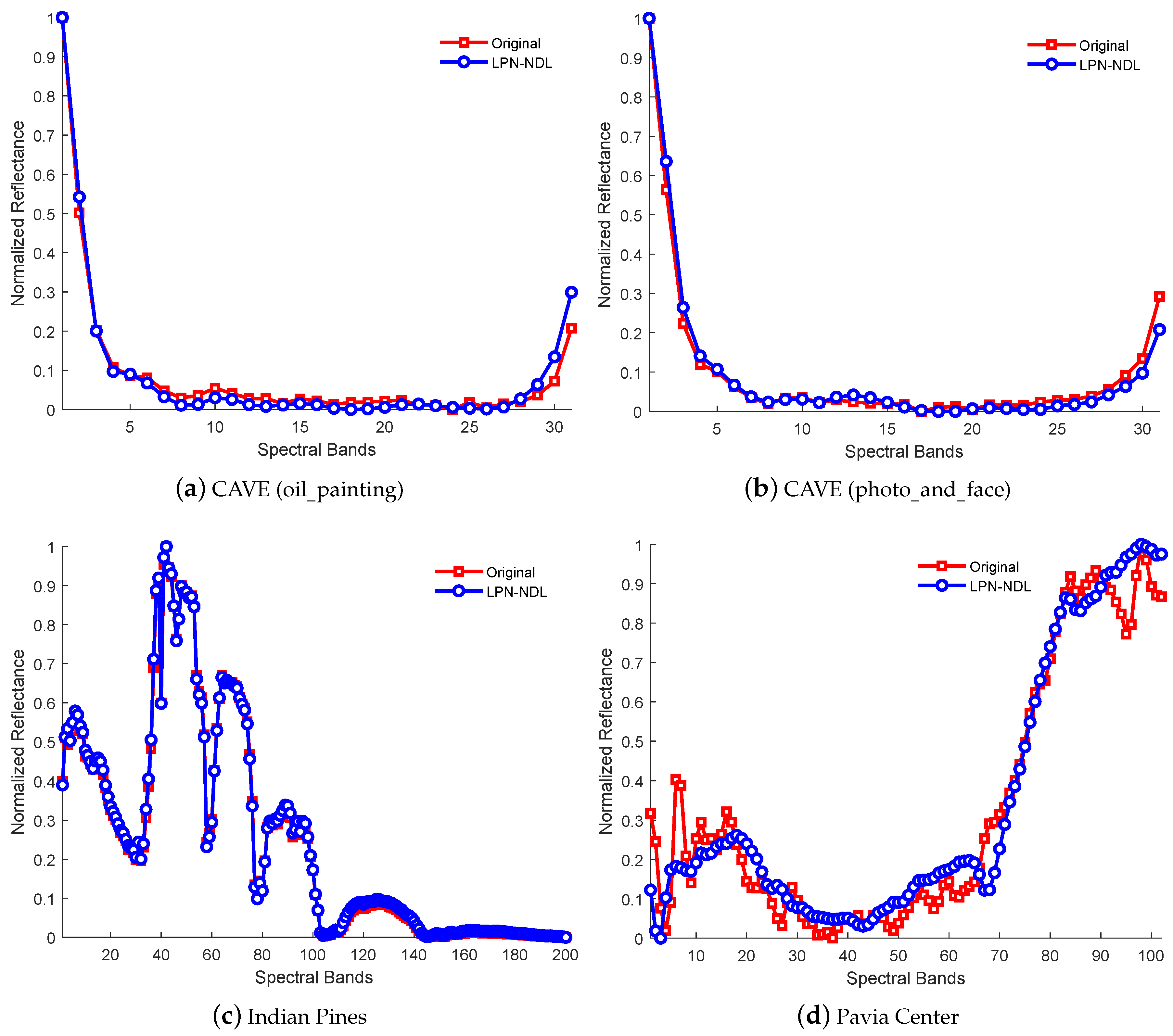
Third, the LPN-NDL provides better or comparable spectral fidelity compared with the competing methods. It is notable from Table 1 that the SAM of the LPN-NDL is lower than that of other methods. To gain further understanding, Figure 9 plots the spectral signatures of the pixels located at (10,10) in the CAVE (oil${}_{\_}$painting image and photo${}_{\_}$and${}_{\_}$face), Indian Pines and Pavia Center datasets. As shown in Figure 9, the spectral profiles obtained by the LPN-NDL is close to their corresponding ground-truths, demonstrating that the LPN-NDL can effectively preserve useful spectral information of the original HSI. Furthermore, it can be clearly seen that the results of LPN-NDL in Figure 9d are slightly inferior to those in Figure 9a–c. This is due to the fact that the spatial size of the Pavia Center is much smaller than that of the other two datasets and the low-resolution image of the Pavia Center dataset is much blurrier compared to that of the other two datasets. Figure 10 depicts the PSNRs of different bands. It can be seen that the performance of the LPN-NDL becomes relatively stable on the CAVE data when the spectral band number is larger than 5, while the PSNR of LPN-NDL varies with the spectral reflectance on the other two datasets. For instance, it is shown in Figure 10c that the bands with higher intensity gain a higher margin of error than those with lower intensity. In short, the experimental results validate the effectiveness of the proposed LPN-NDL method in super-resolution of hyperspectral data.

3.4.2. Statistical Significance Analysis

We used the Kruskal–Wallis test to further study the statistical significance of the proposed method by comparing its results with those from the single image methods and auxiliary-based methods over the RMSE results of the aforementioned datasets. The Kruskal–Wallis test is a non-parametric approach that compares multiple super-resolution methods on multiple datasets. The aforementioned 14 super-resolution methods and three HSI datasets (i.e., the eight test data in the CAVE, the Indian Pines, and the Pavia Center data) are considered in the Kruskal–Wallis test. All of the competitors are ranked for each dataset, the method with the best performance has rank 1, and the second best one gains rank 2, and so on. In case the methods have the same performance on a certain dataset, all of those methods get their average rank. The null hypothesis of the Kruskal–Wallis test is that all of the methods are equivalent.

In this paper, the p-value equals $2.35\times {10}^{-7}$; therefore, we reject the null hypothesis in terms of the significance level $\alpha =0.05$. To evaluate the difference among the methods, we subsequently performed multiple comparisons to determine which levels distinguish a method from other methods. Figure 11 plots the results of the Kruskal–Wallis test to compare the proposed method with both single image methods and auxiliary-based methods. It can be observed from Figure 11a that the median and inter-quartile ranges of the LPN-NDL are much smaller than those of the competing methods, validating the superiority of the proposed LPN-NDL. Moreover, the graphical presentation of the rank difference between any two methods is depicted in Figure 11b, which demonstrates that there are remarkable differences between the LPN-NDL and almost all of the other methods ($p<0.05$). Based on the above analysis, the proposed LPN-NDL method is significantly better than other methods.

3.4.3. Sensitivity Analysis of the Parameters

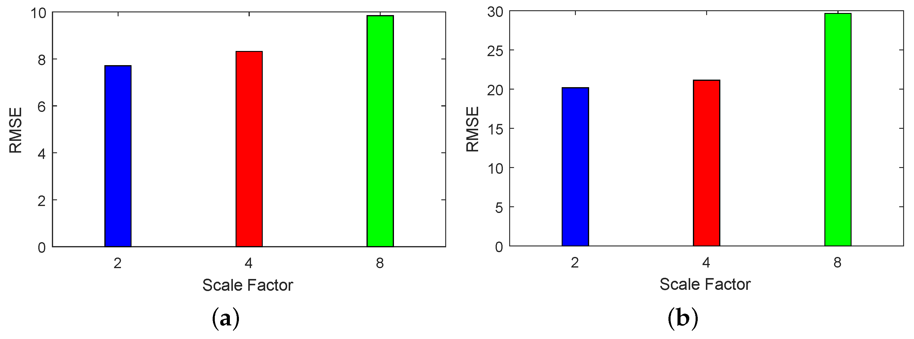
The sensitivity of key parameters (i.e., the up-sampling scale factor S, the number of training epochs, and the regularization parameters $\lambda$ and $\beta$) are evaluated here. Figure 12 shows the impact of the scale factor S on the RMSE for the Indian Pines and Pavia Center datasets. One can see that the RMSE increases with an increasing S. This is due to the fact that super-resolution with a larger scale factor is much more challenging than with a smaller one. However, this does not necessarily mean that the optimum scale factor is simply chosen as 2. The optimum scale factor should be determined by both reconstruction errors and actual requirements in practical applications.

The impact of the number of training epochs is plotted in Figure 13, from which it can be observed that the RMSE increases at the first couple of epochs and then rapidly decreases with increasing number of epochs, and again slowly decreases and finally trends to a certain stable value with increasing number of epochs. As shown in Figure 13, it is suggested that the LPN is trained with more than 400 epochs to achieve stable and effective performance.

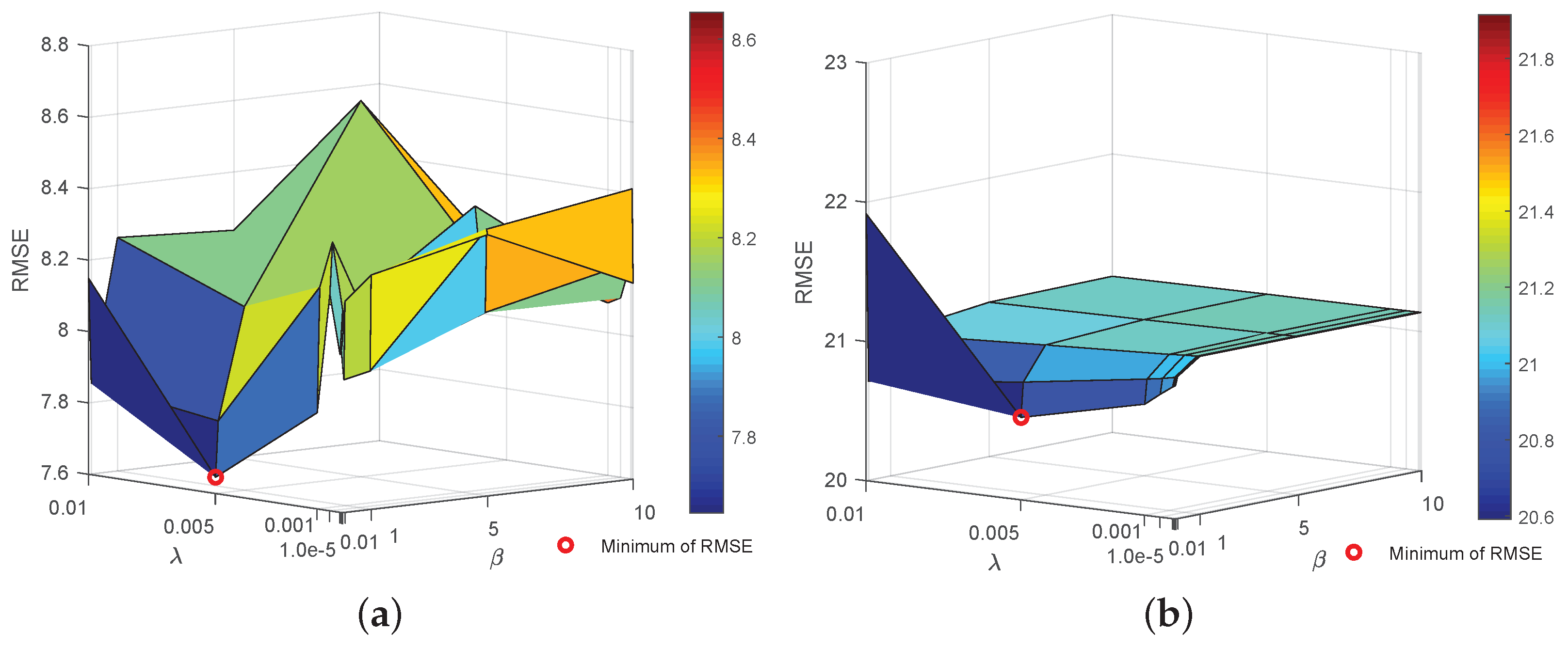
Finally, Figure 14 plots the effect of the regularization parameters $\lambda$ and $\beta$. $\lambda$ is selected from {${10}^{-5}$, $5\times {10}^{-5}$, ${10}^{-4}$, $5\times {10}^{-4}$, 0.001, 0.005, 0.01}, while $\beta$ is chosen from {0.01, 0.1, 1, 5, 10}. It can be seen from Figure 14 that, although the super-resolution performance fluctuates with the change of parameters, the variation is of small amplitude. Moreover, noting that the RMSE obtained with $\lambda \in$ {${10}^{-5}$, $5\times {10}^{-5}$, ${10}^{-4}$, $5\times {10}^{-4}$} and $\beta \in \{0.01,10\}$ is more volatile than that obtained with other ranges, it is better to set the value of $\lambda$ in the range of 0.001 to 0.01, and the value of $\beta$ in the range of 0.1 to 5.

4. Conclusions

In this paper, we have proposed a deep-learning-based hyperspectral super-resolution method to reconstruct a high-resolution HSI from a low-resolution HSI. The proposed LPN-NDL method designs an LPN model to enhance the spatial resolution followed by a NDL method to preserve the spectral information. Compared to most existing super-resolution methods, a notable advantage of the proposed LPN-NDL is that it does not require any auxiliary images (e.g., PAN or MSI) of the same scene. Moreover, by embedding multiple transposed convolutional layers, the LPN-NDL does not need any pre-processing (e.g., bicubic interpolation) to upscale the low-resolution image to the desired size, and the non-negative constraint is added to the spectral reconstruction step to obey the physical reality. Experimental results on three hyperspectral datasets show that the LPN-NDL can provide smaller errors than the competing methods in most cases. A probable future research direction is to improve the proposed method by further avoiding overfitting. How to extend the proposed method to other application areas (e.g., hyperspectral unmixing and classification) is also a future research topic.

References

- Fauvel, M.; Tarabalka, Y.; Benediktsson, J.A.; Chanussot, J.; Tilton, J.C. Advances in spectral-spatial classification of hyperspectral images. Proc. IEEE 2013, 101, 652–675. [Google Scholar] [CrossRef]
- Du, B.; Zhao, R.; Zhang, L.; Zhang, L. A spectral-spatial based local summation anomaly detection method for hyperspectral images. Signal Process. 2016, 124, 115–131. [Google Scholar] [CrossRef]
- Ghamisi, P.; Yokoya, N.; Li, J.; Liao, W.; Liu, S.; Plaza, J.; Rasti, B.; Plaza, A. Advances in hyperspectral image and signal processing: A comprehensive overview of the state of the art. IEEE Geosci. Remote Sens. Mag. 2017, 5, 37–78. [Google Scholar] [CrossRef]
- Gao, D.; Hu, Z.; Ye, R. Self-dictionary regression for hyperspectral image super-resolution. Remote Sens. 2018, 10, 1574. [Google Scholar] [CrossRef]
- Sun, W.; Jiang, M.; Li, W.; Liu, Y. A symmetric sparse representation based band selection method for hyperspectral imagery classification. Remote Sens. 2016, 8, 238. [Google Scholar] [CrossRef]
- Wang, Z.; Zhu, R.; Fukui, K.; Xue, J.H. Cone-based joint sparse modelling for hyperspectral image classification. Signal Process. 2018, 144, 417–429. [Google Scholar] [CrossRef]
- Liu, X.; Sun, Q.; Meng, Y.; Fu, M.; Bourennane, S. Hyperspectral image classification based on parameter-optimized 3D-CNNs combined with transfer learning and virtual samples. Remote Sens. 2018, 10, 1425. [Google Scholar] [CrossRef]
- Du, B.; Wang, S.; Wang, N.; Zhang, L.; Tao, D.; Zhang, L. Hyperspectral signal unmixing based on constrained non-negative matrix factorization approach. Neurocomputing 2016, 204, 153–161. [Google Scholar] [CrossRef]
- Arun, P.; Buddhiraju, K.; Porwal, A. CNN based sub-pixel mapping for hyperspectral images. Neurocomputing 2018, 311, 51–64. [Google Scholar] [CrossRef]
- Uezato, T.; Fauvel, M.; Dobigeon, N. Hyperspectral image unmixing with LiDAR data-aided spatial regularization. IEEE Trans. Geosci. Remote Sens. 2018, 56, 4098–4108. [Google Scholar] [CrossRef]
- Gao, L.; Yao, D.; Li, Q.; Zhuang, L.; Zhang, B.; Bioucas-Dias, J. A new low-rank representation based hyperspectral image denoising method for mineral mapping. Remote Sens. 2017, 9, 1145. [Google Scholar] [CrossRef]
- Yuan, Q.; Zhang, Q.; Li, J.; Shen, H.; Zhang, L. Hyperspectral image denoising employing a spatial-spectral deep residual convolutional neural network. IEEE Trans. Geosci. Remote Sens. 2018, 1–14. [Google Scholar] [CrossRef]
- Makki, I.; Younes, R.; Francis, C.; Bianchi, T.; Zucchetti, M. A survey of landmine detection using hyperspectral imaging. ISPRS J. Photogramm. Remote Sens. 2017, 124, 40–53. [Google Scholar] [CrossRef]
- Dong, Y.; Du, B.; Zhang, L.; Hu, X. Hyperspectral target detection via adaptive information-theoretic metric learning with local constraints. Remote Sens. 2018, 10, 1415. [Google Scholar] [CrossRef]
- Sun, W.; Tian, L.; Xu, Y.; Du, B.; Du, Q. A randomized subspace learning based anomaly detector for hyperspectral imagery. Remote Sens. 2018, 10, 417. [Google Scholar] [CrossRef]
- Loncan, L.; de Almeida, L.B.; Bioucas-Dias, J.M.; Briottet, X.; Chanussot, J.; Dobigeon, N.; Fabre, S.; Liao, W.; Licciardi, G.A.; Simoes, M.; et al. Hyperspectral pansharpening: a review. IEEE Geosci. Remote Sens. Mag. 2015, 3, 27–46. [Google Scholar] [CrossRef]
- Yue, L.; Shen, H.; Li, J.; Yuan, Q.; Zhang, H.; Zhang, L. Image super-resolution: The techniques, applications, and future. Signal Process. 2016, 128, 389–408. [Google Scholar] [CrossRef]
- Wei, Y.; Yuan, Q.; Shen, H.; Zhang, L. Boosting the accuracy of multispectral image pansharpening by learning a deep residual network. IEEE Geosci. Remote Sens. Lett. 2017, 14, 1795–1799. [Google Scholar] [CrossRef]
- Yuan, Q.; Wei, Y.; Meng, X.; Shen, H.; Zhang, L. A multiscale and multidepth convolutional neural network for remote sensing imagery pan-sharpening. IEEE J. Sel. Top. Appl. Earth Obs. Remote Sens. 2018, 11, 978–989. [Google Scholar] [CrossRef]
- Simoes, M.; Bioucas-Dias, J.; Almeida, L.B.; Chanussot, J. Hyperspectral image superresolution: An edge-preserving convex formulation. In Proceedings of the 2014 IEEE International Conference on Image Processing (ICIP), Paris, France, 27–30 October 2014; pp. 1–5. [Google Scholar]
- Wei, Q.; Dobigeon, N.; Tourneret, J.Y. Bayesian fusion of multi-band images. IEEE J. Sel. Top. Signal Process. 2015, 9, 1117–1127. [Google Scholar] [CrossRef]
- Yokoya, N.; Yairi, T.; Iwasaki, A. Coupled nonnegative matrix factorization unmixing for hyperspectral and multispectral data fusion. IEEE Trans. Geosci. Remote Sens. 2012, 50, 528–537. [Google Scholar] [CrossRef]
- Huang, B.; Song, H.; Cui, H.; Peng, J.; Xu, Z. Spatial and spectral image fusion using sparse matrix factorization. IEEE Trans. Geosci. Remote Sens. 2014, 52, 1693–1704. [Google Scholar] [CrossRef]
- Akhtar, N.; Shafait, F.; Mian, A. Sparse spatio-spectral representation for hyperspectral image super-resolution. In European Conference on Computer Vision; Springer: Cham, Switzerland, 2014; pp. 63–78. [Google Scholar]
- Fang, L.; Zhuo, H.; Li, S. Super-resolution of hyperspectral image via superpixel-based sparse representation. Neurocomputing 2018, 273, 171–177. [Google Scholar] [CrossRef]
- Dong, W.; Fu, F.; Shi, G.; Cao, X.; Wu, J.; Li, G.; Li, X. Hyperspectral image super-resolution via non-negative structured sparse representation. IEEE Trans. Image Process. 2016, 25, 2337–2352. [Google Scholar] [CrossRef] [PubMed]
- Ling, F.; Du, Y.; Xiao, F.; Li, X. Subpixel land cover mapping by integrating spectral and spatial information of remotely sensed imagery. IEEE Geosci. Remote Sens. Lett. 2012, 9, 408–412. [Google Scholar] [CrossRef]
- Zhang, Y.; Du, Y.; Ling, F.; Fang, S.; Li, X. Example-based super-resolution land cover mapping using support vector regression. IEEE J. Sel. Top. Appl. Earth Obs. Remote Sens. 2014, 7, 1271–1283. [Google Scholar] [CrossRef]
- Lanaras, C.; Baltsavias, E.; Schindler, K. Advances in hyperspectral and multispectral image fusion and spectral unmixing. ISPRS Int. Arch. Photogramm. Remote Sens. Spat. Inf. Sci. 2015, XL-3/W3, 451–458. [Google Scholar] [CrossRef]
- Wang, L.; Wang, P.; Zhao, C. Producing subpixel resolution thematic map from coarse imagery: MAP algorithm-based super-resolution recovery. IEEE J. Sel. Top. Appl. Earth Obs. Remote Sens. 2016, 9, 2290–2304. [Google Scholar] [CrossRef]
- Zhang, Y.; Xue, X.; Wang, T.; He, M. A hybrid subpixel mapping framework for hyperspectral images using collaborative representation. IEEE J. Sel. Top. Appl. Earth Obs. Remote Sens. 2017, 10, 5073–5086. [Google Scholar] [CrossRef]
- Zhang, L.; Zhang, L.; Du, B. Deep learning for remote sensing data: A technical tutorial on the state of the art. IEEE Geosci. Remote Sens. Mag. 2016, 4, 22–40. [Google Scholar] [CrossRef]
- He, Z.; Liu, H.; Wang, Y.; Hu, J. Generative adversarial networks-based semi-supervised learning for hyperspectral image classification. Remote Sens. 2017, 9, 1042. [Google Scholar] [CrossRef]
- Wu, S.; Xu, J.; Zhu, S.; Guo, H. A deep residual convolutional neural network for facial keypoint detection with missing labels. Signal Process. 2018, 144, 384–391. [Google Scholar] [CrossRef]
- Khan, M.J.; Khan, H.S.; Yousaf, A.; Khurshid, K.; Abbas, A. Modern trends in hyperspectral image analysis: A review. IEEE Access 2018, 6, 14118–14129. [Google Scholar] [CrossRef]
- Dong, C.; Loy, C.C.; He, K.; Tang, X. Image super-resolution using deep convolutional networks. IEEE Trans. Pattern Anal. Mach. Intell. 2016, 38, 295–307. [Google Scholar] [CrossRef] [PubMed]
- Li, Y.; Hu, J.; Zhao, X.; Xie, W.; Li, J. Hyperspectral image super-resolution using deep convolutional neural network. Neurocomputing 2017, 266, 29–41. [Google Scholar] [CrossRef]
- Hu, J.; Li, Y.; Xie, W. Hyperspectral image super-resolution by spectral difference learning and spatial error correction. IEEE Geosci. Remote Sens. Lett. 2017, 14, 1825–1829. [Google Scholar] [CrossRef]
- Yuan, Y.; Zheng, X.; Lu, X. Hyperspectral image superresolution by transfer learning. IEEE J. Sel. Top. Appl. Earth Obs. Remote Sens. 2017, 10, 1963–1974. [Google Scholar] [CrossRef]
- Lai, W.S.; Huang, J.B.; Ahuja, N.; Yang, M.H. Deep laplacian pyramid networks for fast and accurate super-resolution. Proc. IEEE Conf. Comput. Vis. Pattern Recognit. 2017, 2, 5. [Google Scholar]
- Lai, W.S.; Huang, J.B.; Ahuja, N.; Yang, M.H. Fast and accurate image super-resolution with deep laplacian pyramid networks. arXiv, 2017; arXiv:1710.01992. [Google Scholar] [CrossRef]
- Charbonnier, P.; Blanc-Féraud, L.; Aubert, G.; Barlaud, M. Deterministic edge-preserving regularization in computed imaging. IEEE Trans. Image Process. 1997, 6, 298–311. [Google Scholar] [CrossRef] [Green Version]
- Chen, Y.; Nasrabadi, N.M.; Tran, T.D. Hyperspectral image classification via kernel sparse representation. IEEE Trans. Geosci. Remote Sens. 2013, 51, 217–231. [Google Scholar] [CrossRef]
- Boyd, S.; Parikh, N.; Chu, E.; Peleato, B.; Eckstein, J. Distributed optimization and statistical learning via the alternating direction method of multipliers. Found. Trends Mach. Learn. 2010, 3, 1–122. [Google Scholar] [CrossRef]
- Friedman, J.; Hastie, T.; Höfling, H.; Tibshirani, R. Pathwise coordinate optimization. Ann. Appl. Stat. 2007, 1, 302–332. [Google Scholar] [CrossRef]
- Yasuma, F.; Mitsunaga, T.; Iso, D.; Nayar, S.K. Generalized assorted pixel camera: Postcapture control of resolution, dynamic range, and spectrum. IEEE Trans. Image Process. 2010, 19, 2241–2253. [Google Scholar] [CrossRef] [PubMed]
- Baumgardner, M.F.; Biehl, L.L.; Landgrebe, D.A. 220 Band Aviris Hyperspectral Image Data Set: June 12, 1992 Indian Pine Test Site 3; Purdue University: West Lafayette, IN, USA, 2015. [Google Scholar]
- Available online: http://www.cs.columbia.edu/CAVE/databases/multispectral/ (accessed on 23 November 2018).
- Available online: https://purr.purdue.edu/publications/1947/serve/1?el=1 (accessed on 23 November 2018).
- Available online: http://www.ehu.eus/ccwintco/uploads/e/e3/Pavia.mat (accessed on 23 November 2018).
- Zeyde, R.; Elad, M.; Protter, M. On single image scale-up using sparse-representations. In International Conference on Curves and Surfaces; Springer: Berlin/Heidelberg, Germany, 2010; pp. 711–730. [Google Scholar]
- Timofte, R.; De Smet, V.; Van Gool, L. Anchored neighborhood regression for fast example-based super-resolution. In Proceedings of the IEEE International Conference on Computer Vision, Sydney, Australia, 3–6 December 2013; pp. 1920–1927. [Google Scholar]
- Bevilacqua, M.; Roumy, A.; Guillemot, C.; Morel, M.L.A. Low-complexity single-image super-resolution based on nonnegative neighbor embedding. In Proceedings of the British Machine Vision Conference (BMVC), Surrey, UK, 3–7 September 2012. [Google Scholar]
- Chang, H.; Yeung, D.Y.; Xiong, Y. Super-resolution through neighbor embedding. In Proceedings of the 2004 IEEE Computer Society Conference on Computer Vision and Pattern Recognition, Washington, DC, USA, 27 June–2 July 2004; Volume 1, pp. 275–282. [Google Scholar]
- Timofte, R.; De Smet, V.; Van Gool, L. A+: Adjusted anchored neighborhood regression for fast super-resolution. In Asian Conference on Computer Vision; Springer: Cham, Switzerland, 2014; pp. 111–126. [Google Scholar]
- Liao, W.; Huang, X.; Van Coillie, F.; Gautama, S.; Pižurica, A.; Philips, W.; Liu, H.; Zhu, T.; Shimoni, M.; Moser, G.; et al. Processing of multiresolution thermal hyperspectral and digital color data: outcome of the 2014 IEEE GRSS data fusion contest. IEEE J. Sel. Top. Appl. Earth Obs. Remote Sens. 2015, 8, 2984–2996. [Google Scholar] [CrossRef]
- Laben, C.A.; Brower, B.V. Process for Enhancing the Spatial Resolution of Multispectral Imagery Using Pan-Sharpening. U.S. Patent 6,011,875, 4 January 2000. [Google Scholar]
- Aiazzi, B.; Baronti, S.; Selva, M. Improving component substitution pansharpening through multivariate regression of MS + PAN data. IEEE Trans. Geosci. Remote Sens. 2007, 45, 3230–3239. [Google Scholar] [CrossRef]
- Simões, M.; Bioucas-Dias, J.; Almeida, L.B.; Chanussot, J. A convex formulation for hyperspectral image superresolution via subspace-based regularization. IEEE Trans. Geosci. Remote Sens. 2015, 53, 3373–3388. [Google Scholar] [CrossRef]
- Yang, J.; Wright, J.; Huang, T.S.; Ma, Y. Image super-resolution via sparse representation. IEEE Trans. Image Process. 2010, 19, 2861–2873. [Google Scholar] [CrossRef]
- Arbelaez, P.; Maire, M.; Fowlkes, C.; Malik, J. Contour detection and hierarchical image segmentation. IEEE Trans. Pattern Anal. Mach. Intell. 2011, 33, 898–916. [Google Scholar] [CrossRef]
- Kawakami, R.; Matsushita, Y.; Wright, J.; Ben-Ezra, M.; Tai, Y.W.; Ikeuchi, K. High-resolution hyperspectral imaging via matrix factorization. In Proceedings of the IEEE Conference on Computer Vision and Pattern Recognition (CVPR), Colorado Springs, CO, USA, 20–25 June 2011; pp. 2329–2336. [Google Scholar]
- Yokoya, N. Texture-guided multisensor superresolution for remotely sensed images. Remote Sens. 2017, 9, 316. [Google Scholar] [CrossRef]
- Wang, Z.; Bovik, A.C.; Sheikh, H.R.; Simoncelli, E.P. Image quality assessment: from error visibility to structural similarity. IEEE Trans. Image Process. 2004, 13, 600–612. [Google Scholar] [CrossRef] [PubMed]
- Wald, L. Quality of high resolution synthesised images: Is there a simple criterion? In Proceedings of the Third Conference Fusion of Earth Data: Merging Point Measurements, Raster Maps and Remotely Sensed Images, Sophia Antipolis, France, 26–28 January 2000; 99–103; pp. 99–103. [Google Scholar]
- Yuhas, R.H.; Goetz, A.F.; Boardman, J.W. Discrimination among semi-arid landscape endmembers using the spectral angle mapper (SAM) algorithm. In Proceedings of the Summaries of the Third Annual JPL Airborne Geoscience Workshop, Pasadena, CA, USA, 1–5 June 1992; pp. 147–149. [Google Scholar]
- Gabarda, S.; Cristóbal, G. Blind image quality assessment through anisotropy. J. Opt. Soc. Am. A 2007, 24, B42–B51. [Google Scholar] [CrossRef]
Figure 1.
Schematic illustration of the proposed hyperspectral image (HSI) super-resolution method.
Figure 2.
General architecture of the deep Laplacian pyramid network (LPN).
Figure 3.
Structure of a recursive block in the feature-embedding sub-network.
Figure 4.
The high-resolution Red Green Blue (RGB) images of the eight test data from the CAVE dataset. (a) balloons; (b) egyptianstatue; (c) face; (d) fakeandreallemonslices; (e) fakeandrealstrawberries; (f) oilpainting; (g) photoandface and (h) pompoms.
Figure 5.
The high-resolution RGB images of (a) Indian Pines dataset and (b) Pavia Center dataset.
Figure 6.
Reconstructed image of the oilpainting from the CAVE dataset. (a) original image; (b) the low-resolution image; (c) bicubic; (d) Zeyde; (e) anchored neighborhood regression (ANR), (f) neighbor embedding with least squares (NE + LS), (g) neighbor embedding with non-negative least squares (NE + NNLS), (h) neighbor embedding with locally linear embedding (NE + LLE), (i) A+, (j) super-resolution convolutional neural network (SRCNN); (k) deep Laplacian pyramid network and non-negative dictionary learning (LPN-NDL); (l) coupled non-negative matrix factorization (CNMF); (m) guided filter principal component analysis (GFPCA); (n) Gram-Schmidt spectral sharpening (GS); (o) adaptive GS (GSA) and (p) HySure.
Figure 7.
Reconstructed image of the Indian Pines dataset. (a) original image; (b) the low-resolution image; (c) bicubic; (d) Zeyde; (e) ANR; (f) NE + LS; (g) NE + NNLS; (h) NE + LLE; (i) A+; (j) SRCNN; (k) LPN-NDL; (l) CNMF; (m) GFPCA; (n) GS; (o) GSA and (p) HySure.
Figure 8.
Reconstructed image of the Pavia Center dataset. (a) original image; (b) the low-resolution image; (c) bicubic; (d) Zeyde; (e) ANR; (f) NE + LS; (g) NE + NNLS; (h) NE + LLE; (i) A+; (j) SRCNN; (k) LPN-NDL; (l) CNMF; (m) GFPCA; (n) GS; (o) GSA and (p) HySure.
Figure 9.
Spectral signatures of pixels located at (10,10) in (a) CAVE (oilpainting image); (b) CAVE (photoandface); (c) Indian Pines; and (d) Pavia Center datasets.
Figure 10.
Peak signal-to-noise ratios (PSNRs) of different bands in (a) CAVE (oilpainting image); (b) CAVE (photoandface); (c) Indian Pines; and (d) Pavia Center datasets.
Figure 11.
Results of the Kruskal–Wallis test to compare the proposed method with both single image methods and auxiliary-based methods. (a) box-plot of the Kruskal–Wallis test and (b) graphical presentation of the rank difference between any two methods.
Figure 12.
Impact of the up-sampling scale factor S on the RMSE for (a) Indian Pines and (b) Pavia Center datasets.
Figure 13.
Impact of the training epochs on the RMSE for (a) Indian Pines and (b) Pavia Center datasets.
Figure 14.
Impact of the parameters and on the RMSE for (a) Indian Pines and (b) Pavia Center datasets.