Examining the Performance of PARACUDA-II Data-Mining Engine versus Selected Techniques to Model Soil Carbon from Reflectance Spectra

 , ,
, , 
Abstract
:1. Introduction
2. Materials and Methods
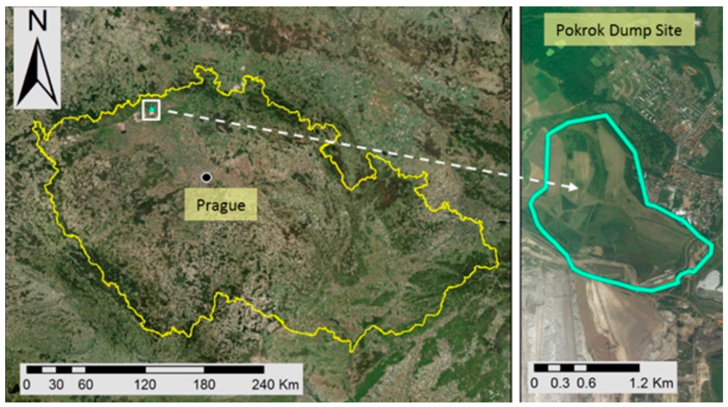
2.1. Experimental Site, Soil Sampling and Analysis
2.2. Soil Spectra Measurement
2.3. Spectra Preprocessing for Selected Data-Mining Techniques
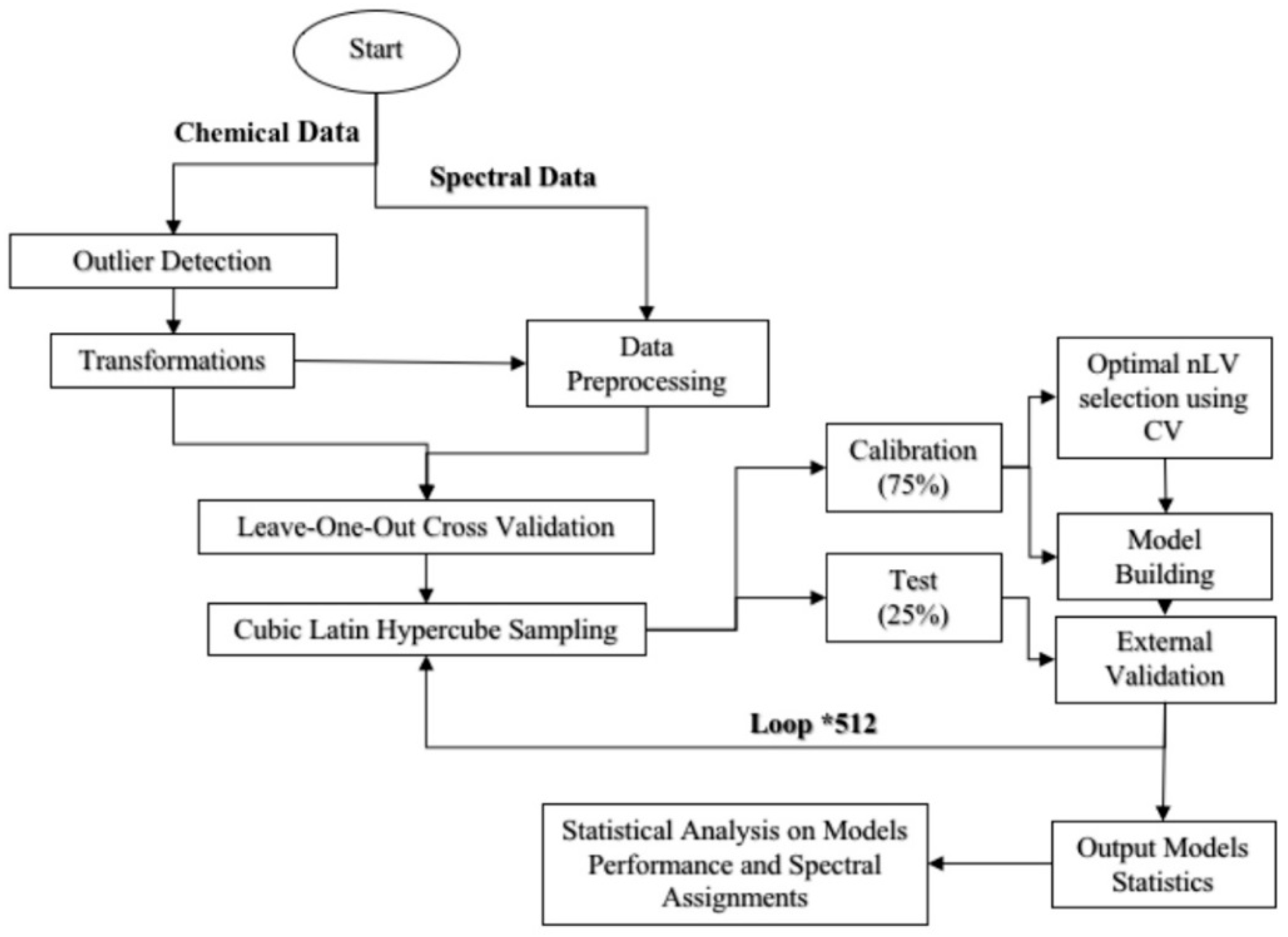
2.4. Development of Calibration Models for Selected Data-Mining Techniques
2.4.1. Partial Least Square Regression (PLSR)
2.4.2. Random Forest (RF)
2.4.3. Boosted Regression Trees (BRT)
2.4.4. Support Vector Machine Regression (SVMR)
2.4.5. Memory Based Learning (MBL)
2.4.6. PARACUDA-II®
2.5. Performance of Models
3. Results
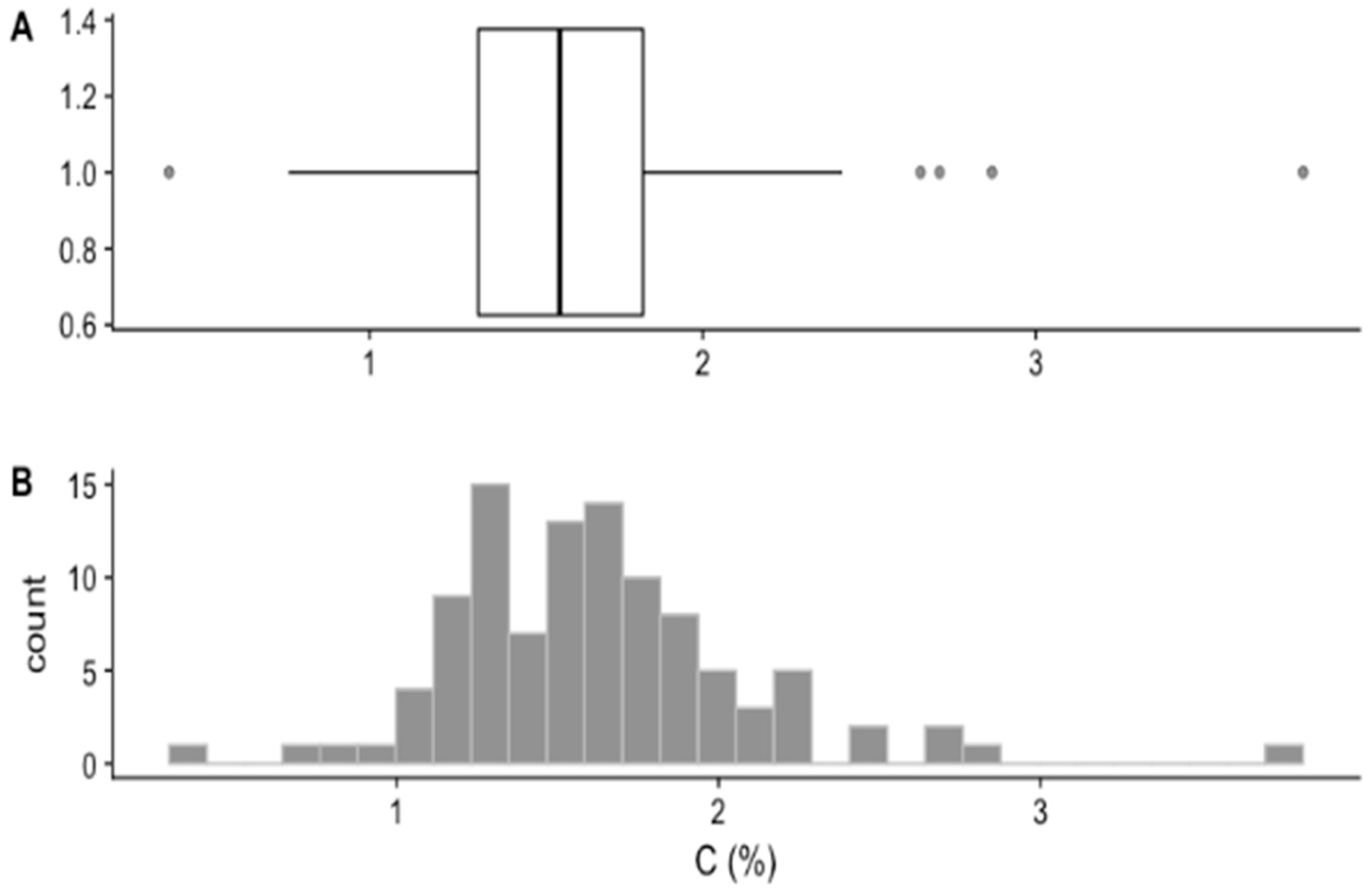
3.1. Soil Cox Statistics
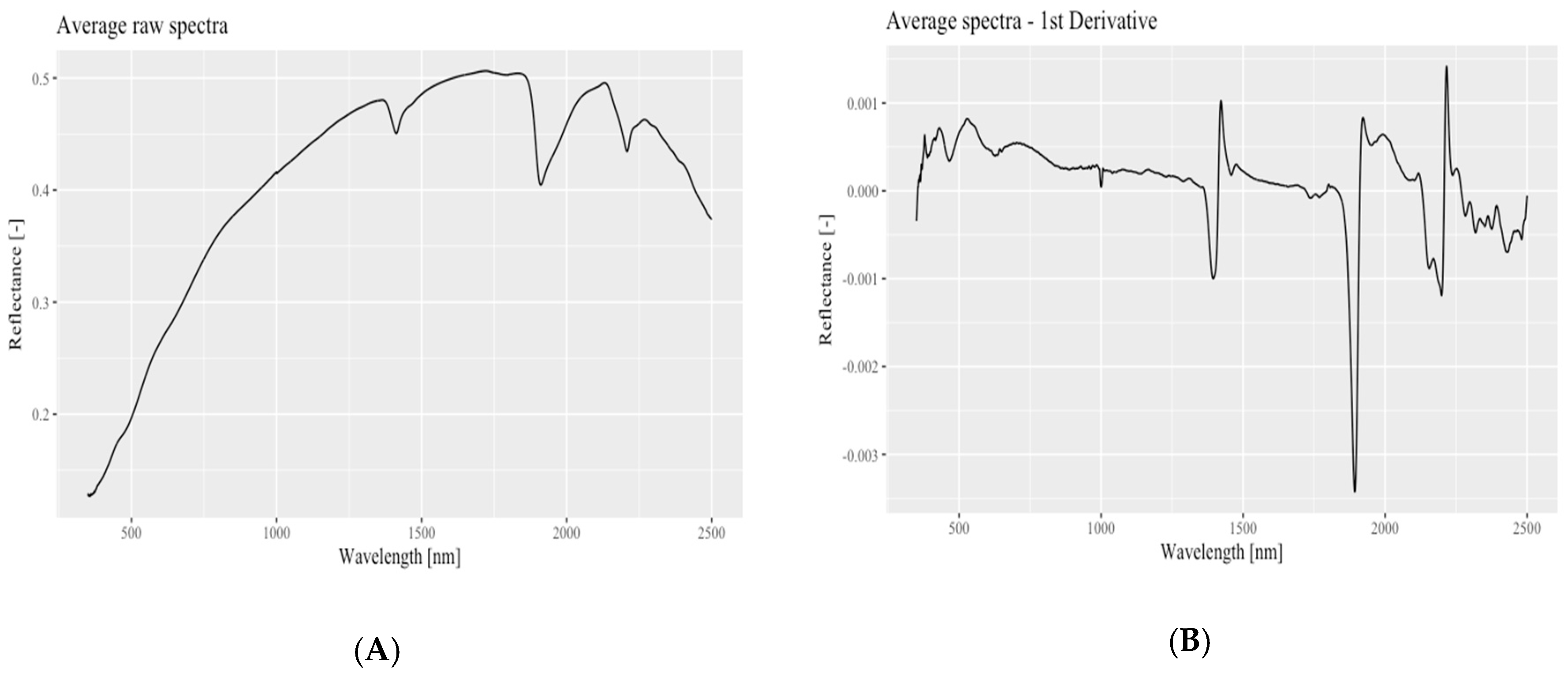
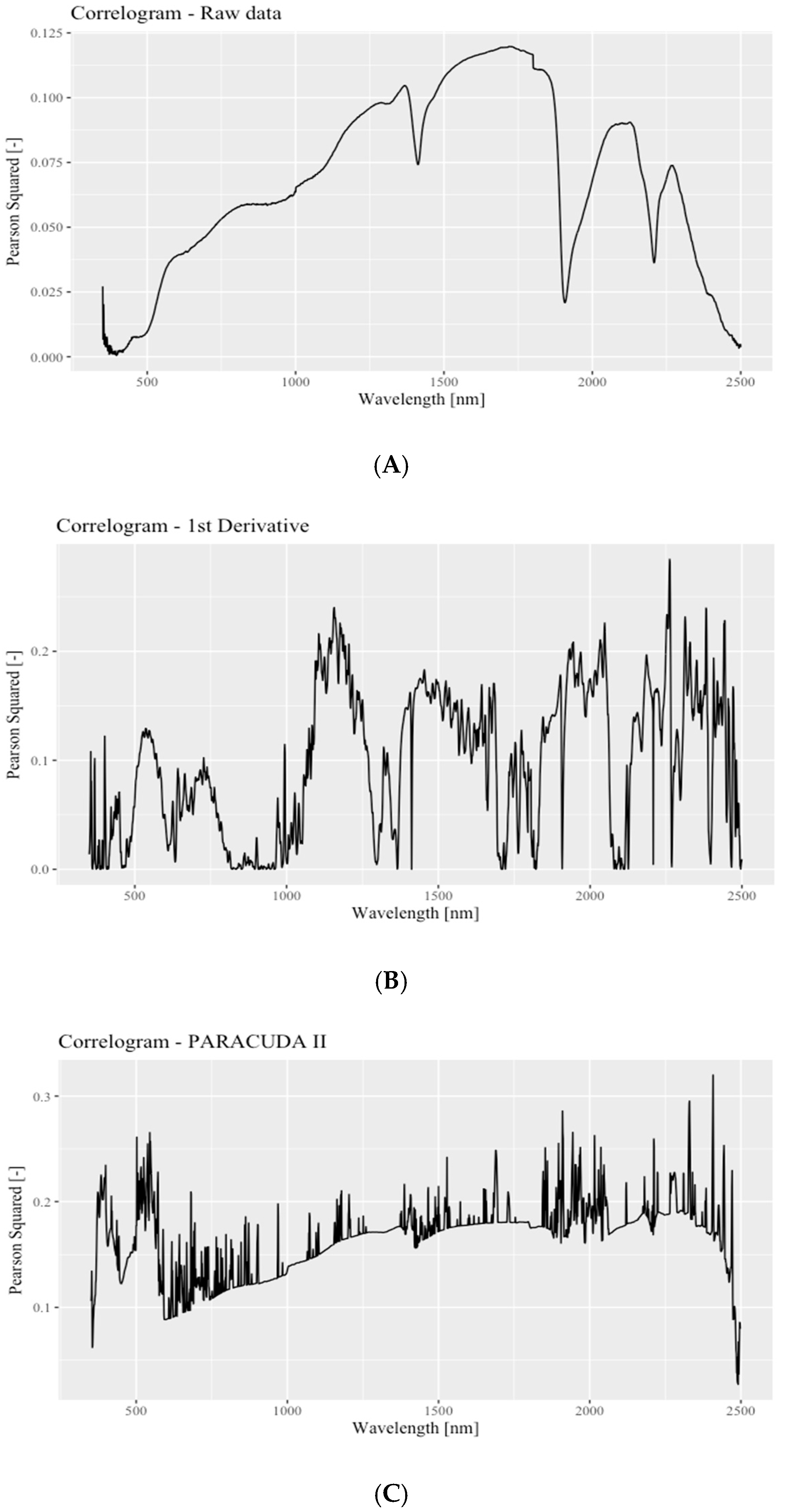
3.2. Soil Spectral Response
3.3. Calibration Model Performance
4. Discussion
5. Summary and Conclusions
Author Contributions
Funding
Acknowledgments
Conflicts of Interest
References
- Smith, P. Monitoring and verification of soil carbon changes under Article 3.4 of the Kyoto Protocol. Soil Use Manag. 2004, 20, 264–270. [Google Scholar] [CrossRef]
- Ben-Dor, E.; Banin, A. Near-Infrared Analysis as a Rapid Method to Simultaneously Evaluate Several Soil Properties. Soil Sci. Soc. Am. J. 1995, 59, 364–372. [Google Scholar] [CrossRef]
- Reeves, J.B., III. Near-versus Mid-Infrared diffuse reflectance spectroscopy for soil analysis emphasizing carbon and laboratory versus on-site analysis: Where are we and what needs to be done? Geoderma 2010, 158, 3–14. [Google Scholar] [CrossRef]
- Ben-Dor, E.; Patkin, K.; Banin, A.; Karnieli, A. Mapping of several soil properties using DAIS-7915 hyperspectral scanner data—A case study over clayey soils in Israel. Int. J. Remote Sens. 2002, 23, 1043–1062. [Google Scholar] [CrossRef]
- Mouazen, A.M.; Maleki, M.R.; De Baerdemaeker, J.; Ramon, H. On-line measurement of some selected soil properties using a VIS-NIR sensor. Soil Till. Res. 2007, 93, 13–27. [Google Scholar] [CrossRef]
- Viscarra Rossel, R.A.; Cattle, S.R.; Ortega, A.; Fouad, Y. In situ measurements of soil colour, mineral composition and clay content by vis-NIR spectroscopy. Geoderma 2009, 150, 253–266. [Google Scholar] [CrossRef]
- Viscarra Rossel, R.A.; Walvoort, D.J.J.; McBratney, A.B.; Janik, L.J.; Skjemstad, J.O. Visible, near-infrared, mid-infrared or combined diffuse reflectance spectroscopy for simultaneous assessment of various soil properties. Geoderma 2006, 131, 59–75. [Google Scholar] [CrossRef]
- Ben-Dor, E.; Ong, C.; Lau, I.C. Reflectance measurements of soils in the laboratory: Standards and protocols. Geoderma 2015, 245–246, 112–124. [Google Scholar] [CrossRef]
- Martens, H.; Naes, T. Multivariate Calibration; John Wiley and Sons: Chichester, UK, 1989; p. 419. [Google Scholar]
- Viscarra Rossel, R.A.; Behrens, T. Using data mining to model and interpret soil diffuse reflectance spectra. Geoderma 2010, 158, 46–54. [Google Scholar] [CrossRef]
- Gholizadeh, A.; Boruvka, L.; Vasat, R.; Saberioon, M.M. Comparing different data preprocessing methods for monitoring soil heavy metals based on soil spectral features. Soil Water Res. 2015, 10, 218–227. [Google Scholar] [CrossRef]
- Gholizadeh, A.; Carmon, N.; Ben-Dor, E.; Boruvka, L. Agricultural soil spectral response and properties assessment: Effects of measurement protocol and data mining technique. Remote Sens. 2017, 9, 1078. [Google Scholar] [CrossRef]
- Gholizadeh, A.; Saberioon, M.M.; Boruvka, L.; Vasat, R. A memory-based learning approach as compared to other data mining algorithms for the prediction of soil texture using diffuse reflectance spectra. Remote Sens. 2016, 8, 341. [Google Scholar] [CrossRef]
- Wold, S.; Martens, H.; Wold, H. The multivariate calibration method in chemistry solved by the PLS method. In Matrix Pencils, Lecture Notes in Mathematics; Ruhe, A., Kagstrom, B., Eds.; Springer: Heidelberg, Germany, 1983; Volume 973, pp. 286–293. [Google Scholar]
- Conforti, M.; Castrignanò, A.; Robustelli, G.; Scarciglia, F.; Stelluti, M.; Buttafuoco, G. Laboratory-based Vis-NIR spectroscopy and partial least square regression with spatially correlated errors for predicting spatial variation of soil organic matter content. Catena 2015, 124, 60–67. [Google Scholar] [CrossRef]
- Shibusawa, S.; Imade Anom, S.W.; Sato, S.; Sasao, A.; Hirako, S. Soil mapping using the real-time soil spectrophotometer. In Proceedings of the 3rd European Conference on Precision Agriculture, Agro Montpellier, France, 18–20 June 2001; pp. 497–508. [Google Scholar]
- Gholizadeh, A.; Amin, M.S.M.; Saberioon, M.M.; Boruvka, L. Visible and near infrared reflectance spectroscopy to determine chemical properties of paddy soils. J. Food Agric. Environ. 2013, 11, 859–866. [Google Scholar]
- Chang, C.-W.; Laird, D.A.; Mausbach, M.J.; Hurburgh, C.R., Jr. Near-infrared reflectance spectroscopy–principal components regression analysis of soil properties. Soil Sci. Soc. Am. J. 2001, 65, 480–490. [Google Scholar] [CrossRef]
- Shepherd, K.D.; Walsh, M.G. Development of reflectance spectral libraries for characterization of soil properties. Soil Sci. Soc. Am. J. 2002, 66, 988–998. [Google Scholar] [CrossRef]
- Bilgili, A.V.; Van Es, H.M.; Akbas, F.; Durak, A.; Hively, W.D. Visible-near infrared reflectance spectroscopy for assessment of soil properties in a semi-arid area of Turkey. J. Arid Environ. 2010, 74, 229–238. [Google Scholar] [CrossRef]
- Mouazen, A.M.; Kuang, B.; De Baerdemaeker, J.; Ramon, H. Comparison among principal component, partial least squares and back propagation neural network analyses for accuracy of measurement of selected soil properties with visible and near infrared spectroscopy. Geoderma 2010, 158, 23–31. [Google Scholar] [CrossRef]
- Kuang, B.; Tekin, Y.; Mouazen, A.M. Comparison between artificial neural network and partial least squares for on-line visible and near infrared spectroscopy measurement of soil organic carbon, pH and clay content. Soil Till. Res. 2015, 146, 243–252. [Google Scholar] [CrossRef]
- Araujo, S.R.; Wetterlind, J.; Dematte, J.A.M.; Stenberg, B. Improving the prediction performance of a large tropical vis-NIR spectroscopic soil library from Brazil by clustering into smaller subsets or use of data mining calibration techniques. Eur. J. Soil Sci. 2014, 65, 718–729. [Google Scholar] [CrossRef]
- Sorenson, P.T.; Small, C.; Tappert, M.C.; Quideau, S.A.; Drozdowski, B.; Underwood, A.; Janz, A. Monitoring organic carbon, total nitrogen, and pH for reclaimed soils using field reflectance spectroscopy. Can. J. Soil Sci. 2017, 97, 241–248. [Google Scholar] [CrossRef] [Green Version]
- Morellos, A.; Pantazi, X.E.; Moshou, D.; Alexandridis, T.; Whetton, R.; Tziotzios, G.; Wiebensohn, J.; Bill, R.; Mouazen, A.M. Machine learning based prediction of soil total nitrogen, organic carbon and moisture content by using VIS-NIR spectroscopy. Biosyst. Eng. 2016, 152, 104–116. [Google Scholar] [CrossRef]
- Nawar, S.; Mouazen, A.M. Predictive performance of mobile vis-near infrared spectroscopy for key soil properties at different geographical scales by using spiking and data mining techniques. Catena 2017, 151, 118–129. [Google Scholar] [CrossRef]
- Ramirez-Lopez, L.; Behrens, T.; Schmidt, K.; Stevens, A.; Dematte, J.A.M.; Scholten, T. The spectrum-based learner: A new local approach for modeling soil vis-NIR spectra of complex datasets. Geoderma 2013, 195–196, 268–279. [Google Scholar] [CrossRef]
- Clairotte, M.; Grinand, C.; Kouakoua, E.; Thebault, A.; Saby, N.P.A.; Bernoux, M.; Barthes, B.G. National calibration of soil organic carbon concentration using diffuse infrared reflectance spectroscopy. Geoderma 2016, 276, 41–52. [Google Scholar] [CrossRef]
- Carmon, N.; Ben-Dor, E. An advanced analytical approach for spectral-based modelling of soil properties. Int. J. Emerg. Technol. Adv. Eng. 2017, 7, 90–97. [Google Scholar]
- Vohland, M.; Besold, J.; Hill, J.; Frund, H.C. Comparing different multivariate calibration methods for the determination of soil organic carbon pools with visible to near infrared spectroscopy. Geoderma 2011, 166, 198–205. [Google Scholar] [CrossRef]
- Jensen, J.R. Remote Sensing of the Environment: An Earth Resource Perspective; Prentice Hall: Upper Saddle River, NJ, USA, 2007; p. 525. [Google Scholar]
- Mouazen, A.M.; De Baerdemaeker, J.; Ramon, H. Towards development of on-line soil moisture content sensor using a fibre-type NIR spectrophotometer. Soil Till. Res. 2005, 80, 171–183. [Google Scholar] [CrossRef]
- Shi, T.; Wang, J.; Chen, W.; Wu, G. Improving the prediction of arsenic contents in agricultural soils by combining the reflectance spectroscopy of soils and rice plants. Intl. J. Appl. Earth Obs. Geoinf. 2016, 52, 95–103. [Google Scholar] [CrossRef]
- Ren, H.Y.; Zhuang, D.F.; Singh, A.N.; Pan, J.J.; Qid, D.S.; Shi, R.H. Estimation of As and Cu contamination in agricultural soils around a mining area by reflectance spectroscopy: A case study. Pedosphere 2009, 19, 719–726. [Google Scholar] [CrossRef]
- Song, Y.; Li, F.; Yang, Z.; Ayoko, G.A.; Frost, R.L.; Ji, J. Diffuse reflectance spectroscopy for monitoring potentially toxic elements in the agricultural soils of Changjiang river delta, China. Appl. Clay Sci. 2012, 64, 75–83. [Google Scholar] [CrossRef]
- Gomez, C.; Lagacherie, P.; Coulouma, G. Regional predictions of eight common soil properties and their spatial structures from hyperspectral Vis-NIR data. Geoderma 2012, 189–190, 176–185. [Google Scholar] [CrossRef]
- Mark, H.L.; Tunnell, D. Qualitative near-infrared reflectance analysis using Mahalanobis distances. Anal. Chem. 1985, 57, 1449–1456. [Google Scholar] [CrossRef]
- Shenk, J.S.; Westerhaus, M.O. Population definition, sample selection, and calibration procedure for near infrared reflectance spectroscopy. Crop Sci. 1991, 31, 469–474. [Google Scholar] [CrossRef]
- Duckworth, J. Mathematical data preprocessing. In Near-Infrared Spectroscopy in Agriculture; Roberts, C.A., Workman, J., Jr., Reeves, J.B., III, Eds.; ASA-CSSA-SSSA: Madison, WI, USA, 2004; pp. 115–132. [Google Scholar]
- Vasques, G.M.; Grunwald, S.; Sickman, J.O. Comparison of multivariate methods for inferential modeling of soil carbon using visible/near-infrared spectra. Geoderma 2008, 146, 14–25. [Google Scholar] [CrossRef]
- Yu, X.; Liu, Q.; Wang, Y.; Liu, X.; Liu, X. Evaluation of MLSR and PLSR for estimating soil element contents using visible/near-infrared spectroscopy in apple orchards on the Jiaodong peninsula. Catena 2016, 137, 340–349. [Google Scholar] [CrossRef] [Green Version]
- Brown, D.J.; Shepherd, K.D.; Walsh, M.G.; Mays, M.D.; Reinsch, T.G. Global soil characterization with VNIR diffuse reflectance spectroscopy. Geoderma 2006, 132, 273–290. [Google Scholar] [CrossRef]
- Wold, S.; Sjostrom, M.; Eriksson, L. PLS-regression: A basic tool of chemometrics. Chemom. Intell. Lab. Syst. 2001, 58, 109–130. [Google Scholar] [CrossRef]
- Maleki, M.R.; Mouazen, A.M.; De Keterlaere, B.; Ramon, H.; De Baerdemaeker, J. On-the-go variable-rate phosphorus fertilisation based on a visible and near infrared soil sensor. Biosyst. Eng. 2008, 99, 35–46. [Google Scholar] [CrossRef]
- Gholizadeh, A.; Boruvka, L.; Saberioon, M.M.; Vasat, R. Visible, near-infrared, and mid-infrared spectroscopy applications for soil assessment with emphasis on soil organic matter content and quality: State-of-the-art and key issues. Appl. Spectrosc. 2013, 67, 1349–1362. [Google Scholar] [CrossRef] [PubMed]
- Xie, X.; Pan, X.Z.; Sun, B. Visible and near-infrared diffuse reflectance spectroscopy for prediction of soil properties near a Copper smelter. Pedosphere 2012, 22, 351–366. [Google Scholar] [CrossRef]
- Kuhn, M. Building predictive models in R using the caret Package. J. Stat. Softw. 2008, 28, 1–26. [Google Scholar] [CrossRef]
- Breiman, L. Random forests. Mach. Learn. 2001, 45, 5–32. [Google Scholar] [CrossRef]
- Cutler, A.; Cutler, D.R.; Stevens, J.R. Random Forests; Springer: Boston, MA, USA, 2012; pp. 157–175. [Google Scholar]
- Nawar, S.; Mouazen, A.M. Comparison between Random Forests, Artificial Neural Networks and Gradient Boosted Machines Methods of On-Line Vis-NIR Spectroscopy Measurements of Soil Total Nitrogen and Total Carbon. Sensors 2017, 17, 2428. [Google Scholar] [CrossRef] [PubMed]
- Abdel Rahman, A.M.; Pawling, J.; Ryczko, M.; Caudy, A.A.; Dennis, J.W. Targeted metabolomics in cultured cells and tissues by mass spectrometry: Method development and validation. Anal. Chim. Acta 2014, 845, 53–61. [Google Scholar] [CrossRef] [PubMed]
- Segal, M.; Xiao, Y. Multivariate random forests. WIREs Data Min. Knowl. Discov. 2011, 1, 80–87. [Google Scholar] [CrossRef]
- Prasad, A.M.; Iverson, L.R.; Liaw, A. Newer classification and regression tree techniques: Bagging and random forests for ecological prediction. Ecosystems 2006, 9, 181–199. [Google Scholar] [CrossRef]
- Peters, J.; De Baets, B.; Verhoest, N.E.C.; Samson, R.; Degroeve, S.; De Becker, P.; Huybrechts, W. Random forests as a tool for ecohydrological distribution modelling. Ecol. Modell. 2007, 207, 304–318. [Google Scholar] [CrossRef]
- Caruana, R.; Niculescu-Mizil, A. An Empirical Comparison of Supervised Learning Algorithms. In Proceedings of the 23rd International Conference on Machine Learning, Pittsburgh, PA, USA, 25–29 June 2006; pp. 161–168. [Google Scholar]
- Liaw, A.; Wiener, M. Classification and Regression by Random Forest. R News 2002, 2, 18–22. [Google Scholar]
- Brown, D.J. Using a global VNIR soil-spectral library for local soil characterization and landscape modeling in a 2nd-order Uganda watershed. Geoderma 2007, 140, 444–453. [Google Scholar] [CrossRef]
- Breiman, L.; Friedman, J.; Olshen, R.; Stone, C. Classification and Regression Trees; Wadsworth International Group: Belmont, CA, USA, 1984; p. 358. [Google Scholar]
- Steinberg, D.; Colla, P. CART: Tree-Structured Non-Parametric Data Analysis; Salford Systems: San Diego, CA, USA, 1997. [Google Scholar]
- Friedman, J.H. Greedy function approximation: A gradient boosting machine. Ann. Stat. 2001, 29, 1189–1232. [Google Scholar] [CrossRef]
- Freund, Y.; Schapire, R.E. A decision-theoretic generalization of on-line learning and an application to boosting. J. Comput. Syst. Sci. 1997, 55, 119–139. [Google Scholar] [CrossRef]
- Friedman, J.H.; Meulman, J.J. Multiple additive regression trees with application in epidemiology. Stat. Med. 2003, 22, 1365–1381. [Google Scholar] [CrossRef] [PubMed]
- Friedman, J.; Hastie, T.; Tibshirani, R. Additive logistic regression: A statistical view of boosting. Ann. Stat. 2000, 28, 337–374. [Google Scholar] [CrossRef]
- Ridgeway, G. Gbm: Generalized Boosted Regression Models. Available online: https://CRAN.R-project.org/package=gbm (accessed on 12 May 2018).
- Vapnik, V. The Nature of Statistical Learning Theory; Springer: New York, NY, USA, 1995. [Google Scholar]
- Kovacevic, M.; Bajat, B.; Trivic, B.; Pavlovic, R. Geological units classification of multispectral images by using support vector machines. In Proceedings of the International Conference on Intelligent Networking and Collaborative Systems, New York, NY, USA, 4–6 November 2009; pp. 267–272. [Google Scholar]
- Vapnik, V. Statistical Learning Theory; Wiley-Interscience: New York, NY, USA, 1998. [Google Scholar]
- An, A. Classification methods. In Encyclopedia of Data Warehousing and Mining; Wang, J., Ed.; Idea Group Inc.: New York, NY, USA, 2005; pp. 144–149. [Google Scholar]
- Mitchell, T.M. Machine Learning; McGraw-Hill: New York, NY, USA, 1997; pp. 24–51. [Google Scholar]
- Daelemans, W.; Van den Bosch, A. Memory-Based Language Processing; Cambridge University Press: Cambridge, UK, 2005; p. 189. [Google Scholar]
- Russell, S.; Norvig, P. Artificial Intelligence: A Modern Approach; Prentice Hall, Pearson Education Inc.: Upper Saddle River, NJ, USA, 2003; p. 733. [Google Scholar]
- Ramirez-Lopez, L.; Stevens, A. Resemble: Regression and Similarity Evaluation for Memory-Based Learning in Spectral Chemometrics R Package Version 1.2.2. 2016. Available online: https://cran.r-project.org/web/packages/resemble/resemble.pdf (accessed on 1 June 2018).
- Box, G.E.P.; Cox, D.R. An analysis of transformations. J. R. Stat. Soc. Ser. B (Methodol.) 1964, 1964, 211–252. [Google Scholar]
- Sarathjith, M.C.; Das, B.S.; Wani, S.P.; Sahrawat, K.L. Dependency measures for assessing the covariation of spectrally active and inactive soil properties in diffuse reflectance spectroscopy. Soil Sci. Soc. Am. J. 2014, 78, 1522–1530. [Google Scholar] [CrossRef]
- Kusumo, B.H.; Hedley, M.J.; Hedley, C.B.; Tuohy, M.P.; Arnold, C.G. The use of diffuse reflectance spectroscopy for in situ carbon and nitrogen analysis of pastoral soils. Aust. J. Soil Res. 2008, 46, 623–635. [Google Scholar] [CrossRef]
- Kuang, B.; Mouazen, A.M. Calibration of visible and near infrared spectroscopy for soil analysis at the field scale on three European farms. Eur. J. Soil Sci. 2011, 62, 629–636. [Google Scholar] [CrossRef]
- Ben-Dor, E.; Irons, J.R.; Epema, G.F. Soil reflectance. In Manual of Remote Sensing, Remote Sensing for the Earth Sciences; Rencz, A.N., Ed.; John Wiley & Sons: New York, NY, USA, 1999; pp. 111–188. [Google Scholar]
- Brunet, D.; Barthes, B.G.; Chotte, J.L.; Feller, C. Determination of carbon and nitrogen contents in Alfisols, Oxisols and Ultisols from Africa and Brazil using NIRS analysis: Effects of sample grinding and set heterogeneity. Geoderma 2007, 139, 106–117. [Google Scholar] [CrossRef]
- Gholizadeh, A.; Boruvka, L.; Vasat, R.; Saberioon, M.M.; Klement, A.; Kratina, J.; Tejnecky, V.; Drabek, O. Estimation of potentially toxic elements contamination in anthropogenic soils on a brown coal mining dumpsite by reflectance spectroscopy: A case study. PLoS ONE 2015. [Google Scholar] [CrossRef] [PubMed]
- Jalabert, S.S.M.; Martin, M.P.; Renaud, J.P.; Boulonne, L.; Jolivet, C.; Montanarella, L. Estimating forest soil bulk density using boosted regression modeling. Soil Use Manag. 2010, 26, 516–528. [Google Scholar] [CrossRef]
- Stevens, A.; Udelhoven, T.; Denis, A.; Tychon, B.; Lioy, R.; Van Wesemeal, B. Measuring soil organic carbon in croplands at regional scale using airborne imaging spectroscopy. Geoderma 2010, 158, 32–45. [Google Scholar] [CrossRef] [Green Version]
- Zornoza, R.; Guerrero, C.; Mataix-Solera, J.; Scow, K.M.; Arcenegui, V.; Mataix-Beneyto, J. Near infrared spectroscopy for determination of various physical, chemical and biochemical properties in Mediterranean soils. Soil Biol. Biochem. 2008, 40, 1923–1930. [Google Scholar] [CrossRef] [PubMed] [Green Version]
- Boser, B.E.; Guyon, I.M.; Vapnik, V.N. A training algorithm for optimal margin classifiers. In 5th Annual ACM Workshop on COLT; Haussler, D., Ed.; ACM Press: Pittsburgh, PA, USA, 1992; pp. 144–152. [Google Scholar] [Green Version]
- Gupta, A.; Vasava, H.B.; Das, B.S. Choubey, K. Local modeling approaches for estimating soil properties in selected Indian soils using diffuse reflectance data over visible to near-infrared region. Geoderma 2018, 325, 59–71. [Google Scholar] [CrossRef]
- Carmon, N.; Ben-Dor, E. Mapping Asphaltic Roads’ Skid Resistance Using Imaging Spectroscopy. Remote Sens. 2018, 10, 430. [Google Scholar] [CrossRef]


| Characteristic | Cox (%) |
|---|---|
| Mean | 1.62 |
| Median | 1.57 |
| Min. | 0.40 |
| Max. | 3.80 |
| Std. Dev. | 0.47 |
| CV | 29 |
| Data-Mining Technique | Cox (%) | ||
|---|---|---|---|
| R2 | RMSEp | bias | |
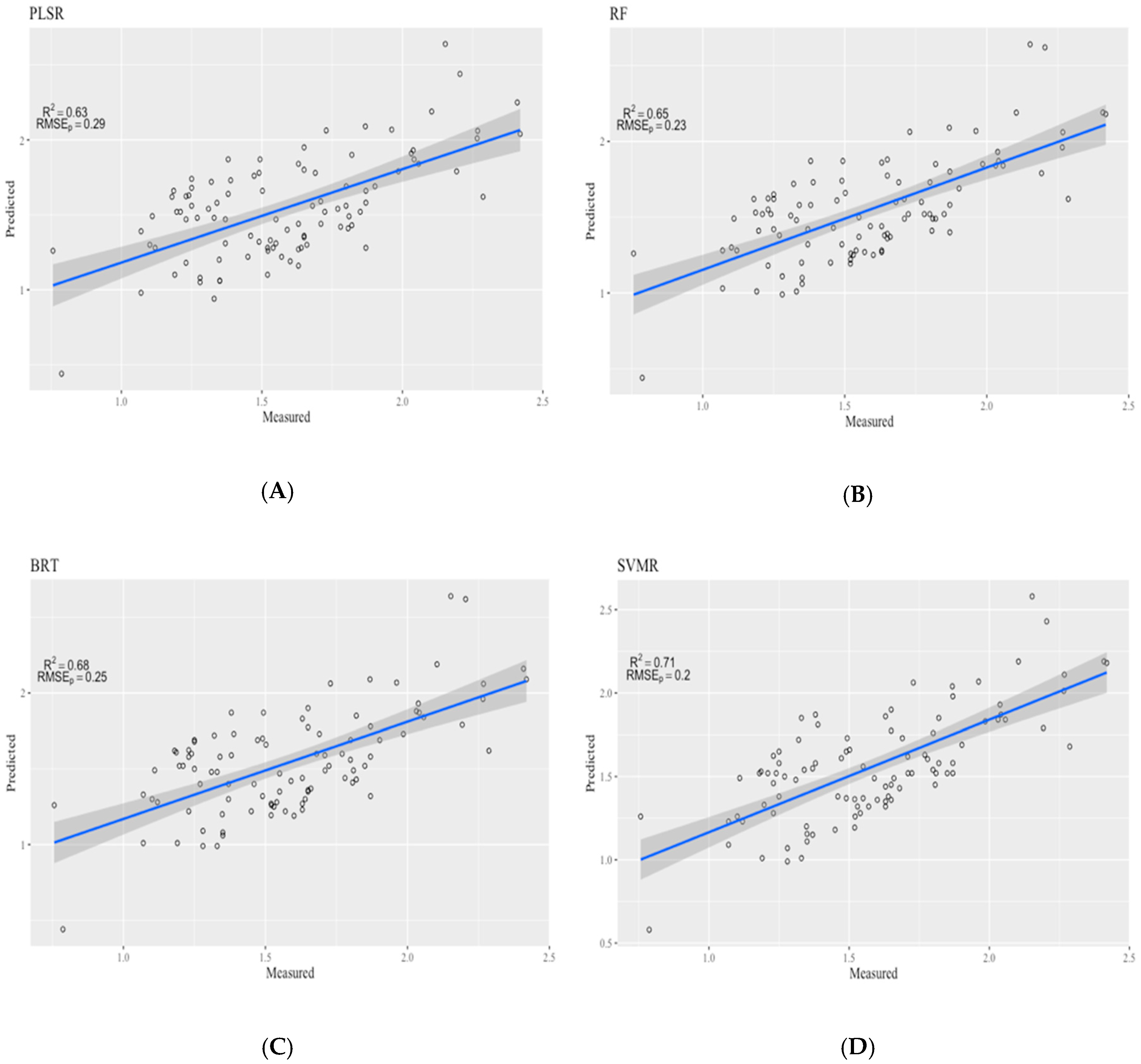
| PLSR | 0.63 | 0.29 | −0.021 |
| RF | 0.65 | 0.23 | −0.020 |
| BRT | 0.68 | 0.25 | −0.017 |
| SVMR | 0.71 | 0.20 | −0.014 |
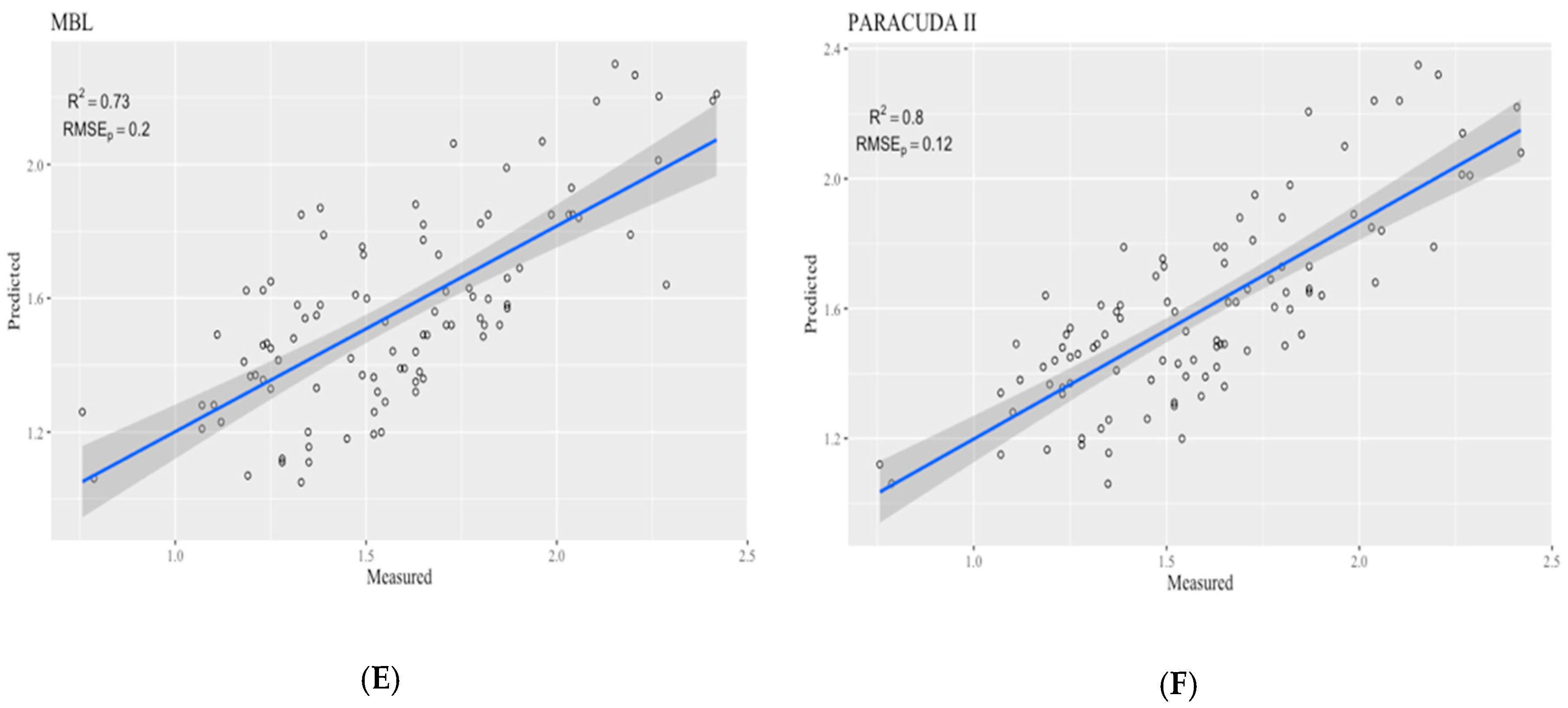
| MBL | 0.73 | 0.20 | −0.013 |
| PARACUDA-II® | 0.80 | 0.12 | 0.003 |
© 2018 by the authors. Licensee MDPI, Basel, Switzerland. This article is an open access article distributed under the terms and conditions of the Creative Commons Attribution (CC BY) license (http://creativecommons.org/licenses/by/4.0/).
Share and Cite
Gholizadeh, A.; Saberioon, M.; Carmon, N.; Boruvka, L.; Ben-Dor, E. Examining the Performance of PARACUDA-II Data-Mining Engine versus Selected Techniques to Model Soil Carbon from Reflectance Spectra. Remote Sens. 2018, 10, 1172. https://doi.org/10.3390/rs10081172
Gholizadeh A, Saberioon M, Carmon N, Boruvka L, Ben-Dor E. Examining the Performance of PARACUDA-II Data-Mining Engine versus Selected Techniques to Model Soil Carbon from Reflectance Spectra. Remote Sensing. 2018; 10(8):1172. https://doi.org/10.3390/rs10081172
Chicago/Turabian StyleGholizadeh, Asa, Mohammadmehdi Saberioon, Nimrod Carmon, Lubos Boruvka, and Eyal Ben-Dor. 2018. "Examining the Performance of PARACUDA-II Data-Mining Engine versus Selected Techniques to Model Soil Carbon from Reflectance Spectra" Remote Sensing 10, no. 8: 1172. https://doi.org/10.3390/rs10081172