Article

Cross-Scale Correlation between In Situ Measurements of Canopy Gap Fraction and Landsat-Derived Vegetation Indices with Implications for Monitoring the Seasonal Phenology in Tropical Forests Using MODIS Data

1
Graduate School of Geography, Clark University, 950 Main St., Worcester, MA 01610, USA
2
Institute at Brown for Environment and Society, Brown University, 85 Waterman St., Providence, RI 02912, USA
3
Department of Environmental Sciences, University of Virginia, 291 McCormick Rd., Charlottesville, VA 22904, USA
*
Author to whom correspondence should be addressed.
Remote Sens. 2018, 10(7), 979; https://doi.org/10.3390/rs10070979
Submission received: 11 May 2018 / Revised: 11 June 2018 / Accepted: 16 June 2018 / Published: 21 June 2018
(This article belongs to the Section Forest Remote Sensing)

Abstract

:
Deciduousness in dry tropical forests results in substantial seasonal changes to canopy gap fractions. The characterization of such structural properties over large areas is necessary for understanding energy and nutrient distribution within forest ecosystems. However, a spatial extrapolation of measurements from relatively few, spatially-concentrated field observations can yield estimated values that have questionable accuracy and precision at regional scales. This paper uses linear regression models to compare measurements of canopy gap fraction from in situ digital cover photography in the dry tropical forest of the Southern Yucatán, Mexico, to measurements of seasonal vegetation change based on three vegetation indices—the Normalized Difference Vegetation Index (NDVI), two-band Enhanced Vegetation Index (EVI2), and the Normalized Difference Water Index (NDWI)—derived from Landsat-7 ETM+ and Landsat-8 Operational Land Imager (OLI) data to gauge the ability of standardized combinations of multispectral reflectance data to accurately describe the intensity of deciduousness that occurs during the dry season. Discrete observations are compared, as well as spatially summarized values at coarser spatial scales. Model R2 values are greater at coarse spatial scales for all vegetation indices. Models of in situ measurements of gap fraction and Landsat NDWI normalized seasonal change exhibit stronger correlation than do models that feature NDVI or EVI2 (R² = 0.751 and Mean Absolute Error = 0.04 after aggregation, R² = 0.552 and MAE = 0.07 for observation-level data). Based on its comparatively strong correlation with field observations, NDWI is adapted to a Moderate Resolution Imaging Spectroradiometer (MODIS) time series and used for spatial extrapolation and the monitoring of canopy conditions. NDWI values derived from MODIS data are regressed against Tropical Rainforest Measuring Misson (TRMM) rainfall data over the period 2000–2011, and the regression results are compared to those of a prior study that used regression to explain the variation of a MODIS EVI using TRMM rainfall data. A MODIS NDWI time series reveals stronger correlation (R² = 0.48 in deciduous forests) with TRMM accumulated (three-month) rainfall data than a MODIS EVI time series. The results indicate that an NDWI time series can accurately describe a variability of canopy leaf abundance during the dry season and could be an alternative basis of long-term monitoring of season phenology in a dry tropical forest.

Graphical Abstract

1. Introduction

The quantification of forest structural properties such as aboveground biomass, canopy height, and canopy gap fraction is key to understanding the role of these ecosystems in a host of processes [1]; from the global carbon cycle [2], to national-scale natural resource policy [3], and plans for the financial commodification of avoided deforestation [4,5,6]. Accurate measurements of forest structural properties can be made from in situ observations, but attempts to extrapolate these properties over larger areas are limited to local extents within a short temporal window [3,7]. In fact, due to technical and financial constraints, many useful in situ measurements cannot be made in a standardized fashion over time, or in some locations at all [8]. However, satellite remote sensing approaches permit large areal extent forest structural measurement given their ability to observe remote locations, and produce large amounts of observations using standardized data capture techniques and information formats [7]. The integration of both in situ and remotely sensed measurements is an ideal way to complement each type of observation, especially for large-area forest assessments [9,10,11].
Multispectral spaceborne sensors collect data at high temporal frequency that can be used to identify the environmental factors that drive changes to forest vegetation phenology over annual cycles and multiple years [12]. Many spectral indices of surface reflectance are sensitive to the chemical and biophysical properties of photosynthetic vegetation, and thus are robust indicators of the abundance and condition of leafy material in the forest canopy [13]. Indices such as the Normalized Difference Vegetation Index (NDVI) [14] and two-band Enhanced Vegetation Index (EVI2) [15] that contrast visible and near-infrared reflectance to provide a composite measurement of photosynthetic production and leaf abundance [16]. Others such as the Normalized Difference Water Index (NDWI) contrast reflectance in the near-infrared and short wave-infrared ranges and are sensitive to moisture [17]. Moderate and coarse spatial resolution remotely sensed data such as observations from the Moderate Resolution Imaging Spectroradiometer (MODIS) onboard the Terra and Aqua platforms, Landsat-7 Enhanced Thematic Mapper (ETM+), and Landsat-8 Operational Land Imager (OLI) offer representative, low, or no-cost observations of forest canopy condition and circumvent logistical barriers to access and ground observation in dense tropical forests [18]. Data at 30-m spatial resolution from Landsat are an attractive option for the relatively fine spatial resolution characterization of forest phenology for many areas, and typically can provide at least one good quality image during cloud-free periods in the region [19]. MODIS data are indispensable for estimation of the timing of important phenological events because of the sensors’ short revisit period, but the 250–1000 m spatial resolution of MODIS products can be too coarse for the accurate and comprehensive characterization of phenology in frontier areas where agricultural deforestation can be small (sub-pixel), and produce a mosaic landscape of differently-aged forest stands [20]. Despite the benefits of spaceborne multispectral sensors for studies of vegetation phenology, they only provide indirect information on the three-dimensional structure of forest, which is valuable for understanding forest structural properties [21]. Particularly for applications in deciduous tropical forests, reflectance-based measurements of biophysical greenness can be used to describe canopy conditions, but would not distinguish between greenness of canopy foliage versus that of sub-canopy vegetation [22].
In dry tropical forests, standardized and repeated observations over time are vital for the accurate measurement of structural parameters. Even with such measurements, phenological processes such as seasonal deciduousness can result in large magnitude differences in observed values of properties such as canopy gap fraction (i.e., the fraction of view through a canopy that is not blocked by foliage or woody plant material) [12,23]. Moreover, in landscapes where the magnitudes of seasonal changes vary substantially on an interannual basis, multiple years of observations are required to characterize a representative range of phenological behavior [12,24,25].
This paper analyzes the relationships at three levels of spatial aggregation between in situ measurements of canopy gap fraction, and three multispectral vegetation indices derived from Landsat data in the Southern Yucatán Peninsula. The findings from that analysis then inform an investigation into the role of precipitation as a driver of deciduous phenology over 11 years in the region, with results compared to prior work that regressed MODIS EVI against rainfall [12] without incorporating in situ or Landsat reflectance data in a capacity beyond reference data. In accomplishing these objectives, the paper: (a) employs digital canopy photography as a way to gather a substantial amount of in situ canopy observations over a large spatial area; (b) evaluates the correspondence of three Landsat-derived vegetation indices with ground observations; (c) considers how the strength of these relationships changes as data are spatially aggregated to increasingly coarser scales; and (d) demonstrates with an analysis of MODIS data that the relative usefulness of the evaluated vegetation indices for describing deciduous phenology that was observed using fine-spatial data also prevails when coarse-scale data are used.

2. Materials and Methods

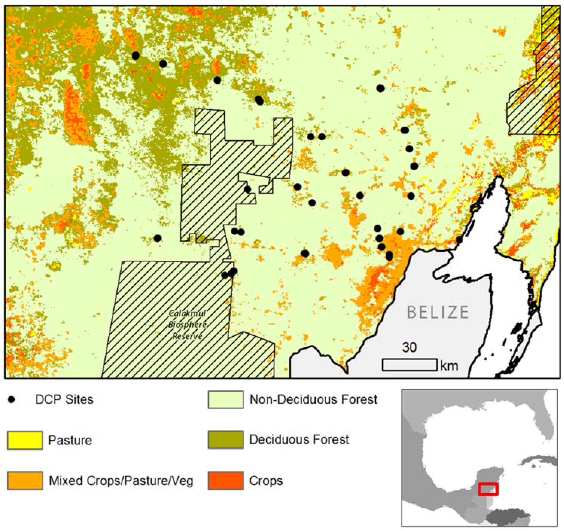
2.1. Study Area Description

This analysis examines the southern Yucatan Peninsula within the rectangular area enclosed by (19.25°, −90.25°) and (17.75°, −87.5°), an area that encompasses the Calakmul and southern Sian Ka’an Biosphere Reserves. The population is concentrated in the coastal areas in and around Chetumal, the capital of Quintana Roo. Slash and burn agriculture, as well as permaculture, is a common livelihood strategy in the central part of the study area, with livestock cultivation more common in the west [26].
Regional topography is characterized by low slope areas along the coast and rolling limestone hills, interspersed with large solution sinks and a seasonally inundated, short stature forest, which is referred to as bajos, and is located farther inland. A number of forest subtypes exist within the region, distinguished on the basis of their stature, topography, and the tendency of common tree species to exhibit deciduousness [27]. These types include selva baja (4–8 m stature, transitional lowland to upland), selva subcaducafolia (6–12 m, upland semi-deciduous), selva mediana (12–25 m, upland semi-evergreen), and selva alta (25+ m, upland semi-evergreen) [28]. Tree species typical of mature forest in the study area include Brosimum alicastrum (ramón), Thouinia canescens, Bursera simaruba, and Manilkara zapota (L.) [27]. These forests exhibit both large seasonal and interannual variability in dry season deciduous leaf loss [29]. Situated south of forests that reliably shed a large portion of their canopy leaves each dry season, and north of forests that rarely shed leaves as a response to water stress [30], the interannual variability in the intensity of deciduousness is correlated with the total accumulated rainfall in the previous months [12].
The mean annual temperature is 27 °C, and mean precipitation ranges from 750–1350 mm/yr. Rainfall exhibits a seasonal pattern, with a dry season (<100 mm) from December to May, as well as a midsummer dry period of ~four weeks in July/August [31,32]. Over the period from 1953 to 2007, annual rainfall measurements from the center of the Calakmul Biosphere Reserve (Zoh Laguna) ranged from a low of 600 mm/yr to a high of 1400 mm/yr, and exhibited a downward trend (approximately −2 mm/yr.), while rainfall during the dry season ranged from 0 mm/yr to 250 mm/yr, and exhibited an upward trend (approximately +2 mm/yr.) [33,34]. Márdero et al. [33] observed a clear decrease in positive rainfall anomalies over this period around Zoh Laguna, including prolonged drought during the 1990s, near forests that exhibit a large interannual range of biophysical greenness, particularly with respect to observed annual minimum values [12]. Due to the local range and trends of climate conditions and canopy deciduousness, the Southern Yucatán is an opportune area to study the variability of forest structural properties over relatively short spatial scales and temporal periods. As interannual variability in the intensity of deciduousness varies with rainfall, monitoring forest canopy conditions is valuable as a regional drought indicator, having important consequences for wildfire risk, habitat quality, and conservation planning [35,36].

2.2. Data Collection

Measurements of canopy gap fraction made with ground photographs are compared to values of vegetation indices derived from Landsat-7 and Landsat-8 data at three levels of spatial aggregation (observation, cluster, and site), revealing how the degree of correspondence changes with the coarsening spatial scale. It is of relevance to MODIS-based monitoring efforts to ascertain whether relationships that are observed to be strong at fine spatial scales, where the unit of analysis corresponds to a discrete photograph and Landsat pixel, maintain such strength at coarse spatial scales (Figure 1). Cross-scale comparisons of canopies exhibiting varying intensities of deciduousness, which are measured as a portion of canopy foliage lost, are made during the late dry season (May), describing spatial variation in canopy gap fraction at approximately the time of minimum leaf abundance.

2.2.1. Field Data Collection

Vertical, sky-oriented digital cover photographs (DCP) are captured using a Nikon COOLPIX L830 with an affixed bubble level, positioned at 1.5 m above ground [37,38,39,40]. DCP are able to be acquired under a wide range of illumination conditions and with low-cost equipment when compared with digital hemispherical photographs [39], allowing for a high number of observations made over a broad area in a relatively short time period. The bubble level is used for precisely orienting the camera, and based on the size and position of the bubble and guides in the level, all of the observations have a zenith angle of less than 5.3 degrees. Photographic exposure varies according to light conditions and openness of the canopy at the site of the observation, ranging from shutter speeds of 1/400 to 1/1500. Immediately following the acquisition of each DCP observation, latitude and longitude is recorded using a Garmin eTrex HC GPS, to within a positional accuracy of 6 m. Field data are collected between Day-Of-Year (DOY) 131 and 146, in May 2015, at 32 sites (Figure 2) located within selva subcaducafolia or selva mediana forests. Data are purposefully collected in forest stands exhibiting different amounts of deciduous leaf loss to provide measurements of canopy conditions across the observed range of deciduousness intensity. Typical canopy height at sites ranges from approximately 6 m to 16 m, with the tallest crowns reaching 20 m. Understory vegetation is present at all but the smallest stature sites, and consists of grasses, shrubs, and in certain locations, ferns. The total number of DCP observations of canopy gap fraction obtained from all of the sites is 376. From this total, 250 DCP observations, at 20 sites, are able to be subsequently matched with spatially co-occurring, quality-screened Landsat Surface Reflectance measurements [41] from the leaf-off period of 2015.
Each site contains between five and 23 observations, and the average number of observations per site is 12.5. In the scalar hierarchy according to which the DCP data are organized, between the broad-extent site scale and the small-extent observation scale, an intermediate-scale unit called a cluster is used to describe conditions over areas of approximately 1000 m² to 10,000 m². In this organizational hierarchy, sites are comprised of clusters, and clusters are comprised of observations. Each site contains between one and six clusters, and the average number of clusters per site is 2.7. In total, there are 54 clusters, and clusters associated with the same site are typically separated from one another by 100s of meters. Within a cluster, observations are typically located 10s of meters away from one another (ranging from 8 m to 75 m). Each cluster contains between one and 11 observations, and the average number of observations per cluster is 4.7. Factors such as illumination conditions, the availability of spatio-temporally corresponding satellite data, and in some cases the area and vertical structure of forest stands affected the number of valid observations per cluster and per site that could be used in the analysis.

2.2.2. Satellite Data Collection

Landsat ETM+ Climate Data Record (values show surface reflectance) data [41,42] and OLI Surface Reflectance data [43,44] from between November 2014 and May 2015 were obtained from the United States Geological Survey’s EarthExplorer. The accuracy of these products is comparable to that of MODIS products [44], and the OLI product benefits from the narrow, aerosol, and cirrus bands implemented in that sensor [45]. Images from the beginning and end of the dry season were analyzed and compared to describe the extent of deciduous leaf loss during the dry season. To maximize the quality of observations at a pixel scale for locations of DCP observations, Landsat reflectance data from multiple dates are acquired and examined for use (Table 1). Data from the period from 2014 DOY 333 to 2015 DOY 017 (29 November to 17 January) are used to characterize leaf-on conditions before the dry season, while data from 2015 DOY 128 to 145 (8 May to 25 May) are used to characterize leaf-off conditions at the end of the dry season. When multiple observations from one of these time periods are available for a pixel, the maximum value from the pre-dry season period or the minimum value from the end of dry season period is used. Leaf-off Landsat data are acquired over a period nearly completely overlapping the period during which DCP observations are made: DCP observations are made between DOY 131 and 146, while the NDWI values to which they were compared are derived from Landsat images acquired between DOY 128 and 145.
MODIS monthly, 1-km resolution vegetation indices data product (13A3 v006) [45] are retrieved from the Reverb tool, courtesy of the NASA Earth Observing System Data and Information System’s Land Processes Distributed Active Archive Center for all of the months from March 2000 to February 2011. Monthly, 0.25-degree resolution multi-satellite rainfall data (3B43) from the Tropical Rainfall Measuring Mission (TRMM) [46] are retrieved via FTP from the Goddard Earth Sciences Data and Information Services Center for all of the months from December 1999 to February 2011. TRMM data incorporate remotely sensed radar observations as well as gauge measurements to estimate rainfall over temporal compositing periods that range from every three hours to monthly.

2.3. Data Processing

Pixels in each DCP observation are classified using an unsupervised k-means classifier into one of nine output categories based on their values in the red, green, and blue bands. On the basis of their spectral similarity to low-brightness wood and leaves or high-brightness sky, these output categories are then aggregated into “plant material” and “gap” categories to produce a binary map of gap fraction for each observation (Figure 3). Use of the k-means classifier to produce a relatively high number of preliminary output classes allows for the identification of the most ambiguous, difficult-to-classify pixels. For 16 DCP observations, or 4% of total, there exists at least one output category from the k-means classifier that includes substantial amounts of plant material close to the point of illumination in the image (typically the sun), as well as darker areas of sky in areas of the photo distant from the sun. These blended output categories are spatially deconstructed prior to aggregation into binary plant/gap images by manually identifying a region around the point of illumination and extracting the portion of the category pixels that constituted plant material and adding these pixels to the aggregate “plant material” category. Each DCP-derived gap fraction value is compared to Landsat vegetation index values from the pixel that contained the GPS coordinates of the DCP observation.
The correlation is measured between DCP gap fraction and three Landsat vegetation indices: NDVI, EVI2, and NDWI. These indices are described in Equations (1)–(3):
NDVI = N I R R e d N I R + R e d ,
EVI 2 = 2.5 N I R R e d ( N I R + 2.4 R e d + 1 ) ,
NDWI = N I R S W I R 2 N I R + S W I R 2 ,
In order to describe the amount of relative change in each of these indices over the course of the dry season, which is used as a proxy measure for dry season deciduous leaf loss, the normalized change of each is derived, according to Equation (4):
Normalized   Seasonal   Change   of   [ INDEX ] = I N D E X p r e d r y   s e a s o n I N D E X e n d o f d r y   s e a s o n I N D E X p r e d r y   s e a s o n ,

2.4. Assessing the Similarity of Ground and Landsat Measurements of Canopy Condition

In situ gap fraction observations and vegetation indices from Landsat measure different properties of the forest canopy, and univariate, ordinary least squares linear regression models are used to assess the correlation between these different sets of observations of canopy conditions. Nine regression models compare correlations involving each of three Landsat vegetation indices, at the observation, cluster, and site levels of spatial aggregation.
An additional regression model is calculated between minimum NDWI values from 2015 and the normalized change of NDWI from 2014–2015, which is a metric defined as the difference between the pre-dry season and end-of-dry-season values of NDWI, divided by the pre-dry-season NDWI value observed during leaf-on conditions. This model indicates the degree to which low index values observed in May can be attributed to change resulting from seasonal deciduousness, rather than simply reflecting values that are consistently low year-round. For each variable comparison, the mean absolute error (MAE) is calculated to describe the distribution of data points around the ordinary least squares best-fit regression equation. MAE is described in Equation (5), where N is the number of observations:
MAE = 1 N i = 1 N | O b s e r v e d i P r e d i c t e d i | ,

2.5. Examination of Rainfall as a Driver of Deciduousness in the Southern Yucatán

After the strength of the relationship between in situ observations of canopy gap fraction and the normalized change of NDVI, EVI2, and NDWI values from Landsat data has been observed, a time series of the vegetation index exhibiting the strongest correlation to ground observations is derived from MOD13A3 data for all of the months from June 2000 to May 2011 (N = 132) in the Southern Yucatán. This time period is examined in order to allow for direct comparison to a prior regression analysis [12] that examined how EVI varied with rainfall. Values of the MODIS vegetation index are explained by TRMM rainfall accumulated over the previous three months using per-pixel linear regression at a 1-km spatial resolution. To provide summary statistics, pixel coefficients of determination are spatially averaged within four forest categories: forests where deciduous leaf loss resulted in >50% decline from observed maximum in 0 years, one to two years, three to four years, five or more years, during the period 2000–2011 [12]. Regressions of the annual normalized seasonal change of the MODIS vegetation index with total annual rainfall, and with total rainfall during the dry season (months January to May) are also performed in order to identify the spatial variation in the drivers of interannual variability in deciduous intensity and highlight variation in expected deciduous behavior under predicted future rainfall regimes of lower annual rainfall and increased dry season rainfall.

3. Results

3.1. Assessing the Validity of Using Late-Dry Season Observations of Canopy as Indicators of Deciduousness

Correlation between the normalized seasonal change of NDWI values from the 2014–2015 dry season and the minimum NDWI value from 2015 at the observation scale had an R² of 0.95, and a MAE of 0.02 (Figure 4).

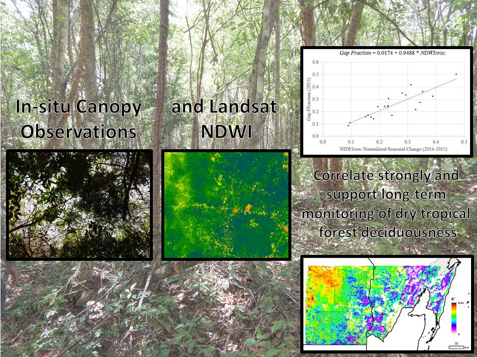
3.2. Comparison of In Situ Gap Fraction and Normalized Seasonal Change of Landsat NDVI

At the observation scale (N = 250), a regression of DCP gap fraction against the normalized seasonal change of NDVI from the Landsat pixel that contained the DCP’s GPS coordinates had an R² of 0.40, and an MAE of 0.09 (Figure 5). At the cluster scale (N = 54), correlation between the average per-cluster DCP gap fraction, and the averaged normalized seasonal change of NDVI from the Landsat pixel that contained the DCP’s GPS coordinates had an R² of 0.48, and an MAE of 0.07. At the site scale (N = 20), correlation between average per-site DCP gap fraction, and the average normalized seasonal change of NDVI from the Landsat pixel that contained the DCP’s GPS coordinates had an R² of 0.57, and an MAE of 0.07.

3.3. Comparison of In Situ Gap Fraction and Normalized Seasonal Change of Landsat EVI2

At the observation scale (N = 250), regression of DCP gap fraction against the normalized seasonal change of EVI2 from the Landsat pixel that contained the DCP’s GPS coordinates had an R² of 0.36, and an MAE of 0.09 (Figure 6). At the cluster scale (N = 54), correlation between average per-cluster DCP gap fraction, and the averaged normalized seasonal change of EVI2 from the Landsat pixel that contained the DCP’s GPS coordinates had an R² of 0.39, and an MAE of 0.08. At the site scale (N = 20), correlation between the average per-site DCP gap fraction, and the average normalized seasonal change of EVI2 from the Landsat pixel that contained the DCP’s GPS coordinates had an R² of 0.41, and an MAE of 0.07.

3.4. Comparison of In Situ Gap Fraction and Normalized Seasonal Change of Landsat NDWI

At the observation scale (N = 250), regression of DCP gap fraction against the normalized seasonal change of NDWI from the Landsat pixel that contained the DCP’s GPS coordinates had an R² of 0.57, and an MAE of 0.07 (Figure 7). At the cluster scale (N = 54), correlation between average per-cluster DCP gap fraction, and the averaged normalized seasonal change of NDWI from the Landsat pixel that contained the DCP’s GPS coordinates had an R² of 0.70, and an MAE of 0.05. At the site scale (N = 20), correlation between an average per-site DCP gap fraction, and the average normalized seasonal change of NDWI from the Landsat pixel that contained the DCP’s GPS coordinates had an R² of 0.75, and an MAE of 0.04.

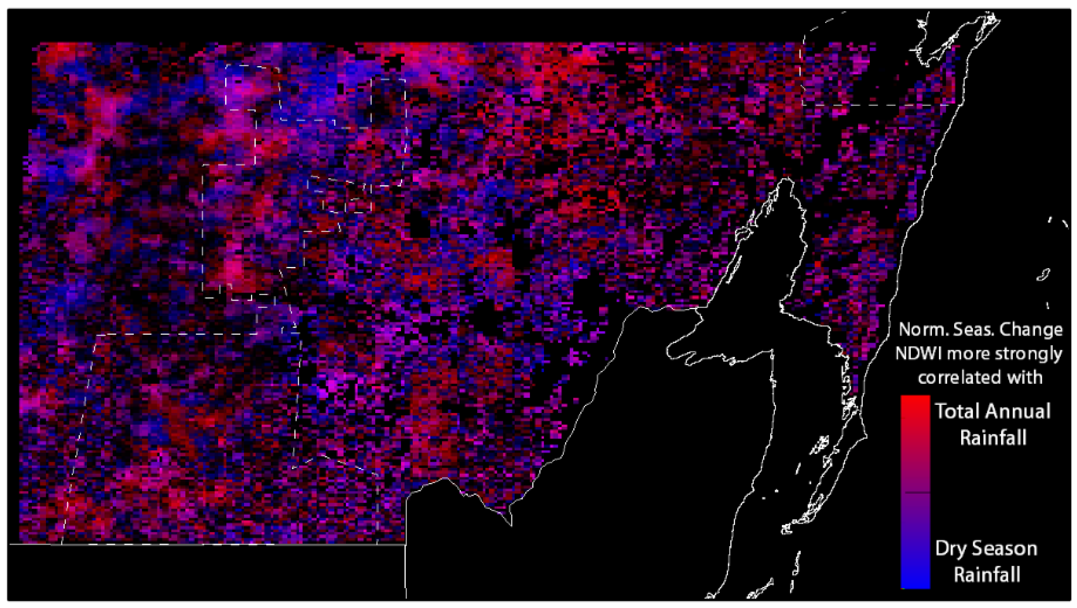
3.5. Modeling MODIS NDWI with TRMM Rainfall

3.5.1. Regressions of Monthly Time Series

Pixels in the west and north of the study area exhibited the strongest correlation between MODIS NDWI, and accumulated, three-month, TRMM rainfall (Figure 8). Average R² values for the forest categories: deciduous in 0 years, deciduous in one to two years, deciduous in three to four years, and deciduous in more than five years (all measured during the period 2000–2011) were 0.29, 0.35, 0.44, and 0.48, respectively. When compared to average R² values from a regression of MODIS EVI and accumulated, three-month TRMM rainfall [14] for the same time period and summary areas, the coefficients of determination from correlations using NDWI were 0.06, 0.06, 0.06, and 0.05 greater, respectively.
The spatial pattern of the 2000–2011 average NDWI normalized seasonal change (Figure 9) strongly resembled that of the coefficient of determination from the regression model using NDWI and TRMM rainfall. The highest values were observed in and to the immediate northwest of the Calakmul Biosphere Reserve, as well as to its northeast. Low values are seen in and around the south of Calakmul, as well as in the northeast of the study area, southwest of the Sian Ka’an Biosphere Reserve.
The mean R2 value for all of the forest pixels in the study area was 0.32, and one standard deviation is equal to 0.14. In Figure 10, the map of forest pixels’ R2 values for the regression between MODIS NDWI and TRMM rainfall was classified into three classes with boundaries at 0.18 and 0.46, equal to µ − 1σ and µ + 1σ respectively, and the mean monthly values of NDWI and TRMM rainfall from 2000 to 2011 were calculated for all of the pixels in each class. The temporal profiles of NDWI values in these sub-regions showed larger differences between the three series than do the profiles of TRMM rainfall. The three classes have similar average maximum NDWI values during the wet season across all of the years, in the range of 0.72 to 0.76, but differed substantially with respect to average minimum NDWI values during the dry season. The low-correlation forests that exhibited the weakest correlation also exhibited the least seasonal change of NDWI, with minimum values between 0.56–0.67. In contrast, in the high-correlation forests, the seasonal change of NDWI was greatest, with minimum values between 0.33–0.48. Forests in these classes experienced varied levels of impact from Hurricane Dean in August 2007 [47]. Low-correlation forests exhibited a sharp decrease in NDWI during the 2007–2008 wet season, while the NDWI of high-correlation forests was relatively unaffected.
The three forest classes had very similar total accumulated, three-month TRMM rainfall in all of the years between 2000–2011. In and between the 2002–2003 and 2006–2007 dry seasons, the high-correlation forests that exhibited the most intense deciduousness are seen to receive more rainfall than the low-correlation, less intense deciduous forests.

3.5.2. Regressions of Annual Time Series

Two regressions modeled the per-pixel relationship between the normalized seasonal change of NDWI and total annual TRMM rainfall (a) in all of the months, and (b) in the dry season months between January and May only. Maps of the coefficients of determination for both regressions (Figure 11) showed low values in areas that exhibited substantial seasonal variability of NDWI, as well as in areas that exhibited little seasonal variability of NDWI. Higher values were seen in central areas, where the intensity of deciduousness exhibited substantial interannual variability, and in these areas, relatively strong correlation was observed. Figure 12 is a composite map of Figure 11a,b, and showed the areas where the interannual variability of deciduousness intensity responded to total annual rainfall, dry season rainfall, both of these variables, or neither.

4. Discussion

The series of regression models that explains DCP gap fraction using normalized seasonal change of NDWI (2014–2015) shows markedly stronger correlation than do the comparisons where NDVI and EVI2 are the independent variable, with a coefficient of determination of 0.55 and a mean absolute error of 0.07 at the observation scale, a coefficient of determination of 0.70 and a mean absolute error of 0.05 at the cluster scale, and a coefficient of determination of 0.75 and a mean absolute error of 0.04 at the site scale. Furthermore, the high coefficient of determination (0.95) and low MAE (0.02) for the regression of normalized seasonal change of NDWI values (2014–2015) and minimum NDWI values (2015) indicates that the spatial variation of minimum NDWI values almost entirely represents spatial variation in the magnitude of seasonal change, rather than seasonally persistent differences in the abundance or condition of vegetation.
Reflectance in the red, near-infrared, and short-wave infrared bands typically increases from the leaf-on period to the leaf-off period, although this increase is much smaller in the near-infrared (10–20%) than the red or short-wave infrared. The regressions for NDVI and EVI2 display heteroskedasticity, with a greater variation of observed gap fraction in locations with a higher seasonal change of vegetation index values, and specifically the presence of observations of low gap fraction where relatively large seasonal change of vegetation indices occur. Previous studies have documented the tendency of shorter stature, quickly-growing species to exhibit a higher intensity dry season deciduousness than mature forests [29,32], and it is posited that these anomalous observations are due to the presence of low stature, sub-canopy vegetation that sheds a very high portion of its leaves and is observable by Landsat but not by the vertically-oriented DCP.
A greater portion of gap fraction variance is explained by all of the Landsat-derived vegetation indices when values are aggregated at coarse-scale sites when compared to discrete observations, The increase in the amount of explained variance that is observed between regressions at coarser scales compared to finer scales can in part be explained by the differing levels of spatial correspondence between the areal footprint over which the different sources of data are acquired. For example, there will always exist a substantial area represented by the Landsat pixel (area ~900 m2) that is outside of the areal extent captured by each DCP observation, and in cases where the DCP observation was obtained within a few meters of the border of the Landsat pixel, there will be a portion of the DCP extent that lies outside of the pixel’s area. Imprecise spatial correspondence will cause substantial random noise at the observation scale, but at coarser scales, the aggregation of values will lead to decreased net impact. Increases in the accuracy of predicted gap fraction with coarser spatial scales suggests that the derivation of NDWI from MODIS reflectance data is a valid methodology to monitor deciduous phenology in dry tropical forest over broad spatial extents at high temporal frequency.
Landsat NDWI, the normalized index of near infrared (NIR) and short wave infrared (SWIR) reflectance, is identified as exhibiting strong correlation with in situ measurements of canopy gap fraction, and linear regression of a monthly, 11-year long, MODIS time series of NDWI against TRMM rainfall data reveals that rainfall data explain a greater portion of MODIS NDWI variance than they did for MODIS EVI variance [12]. Thus, the use of NDWI to parameterize canopy leaf abundance for measuring the intensity of dry season deciduousness is not only supported by closer correlation to in situ observations of canopy, but also allows for the detection of stronger coupling between phenology and rainfall than does the use of visible-NIR indices.
This multi-year regression analysis reveals spatial patterns of forest phenological behavior that point to possible environmental drivers of deciduousness. The map of per-pixel coefficients of determination from the regression of MODIS NDWI against TRMM rainfall (Figure 8) strongly corresponded to a map of average normalized seasonal change of NDWI (Figure 9), indicating that where a relatively high amount of seasonal change occurs, such change is strongly associated with recent amounts of rainfall. Temporal profiles of monthly NDWI and rainfall, averaged over three broad classes of forest-only pixels determined by the degree of correlation between NDWI and rainfall (Figure 10) show that the high-correlation forests exhibit substantially greater seasonal change of NDWI than do forests with lower correlation, but that the rainfall received in these areas is very similar, and in many years, the high correlation–high seasonal change forests received greater rainfall during some wet season months. Since the amount and timing of rainfall is observed to be similar throughout the study area, while the intensity of deciduousness varies substantially, a large amount of lowland forest in the study area should not be expected to exhibit large magnitude changes of deciduousness intensity in response to short-term fluctuations of the amount or timing of rainfall.
Where high intensity deciduousness does occur, it is observed to vary strongly (R² ≤0.83) with interannual changes to the amount of total, or dry season, rainfall in forests inside and to the east of the Calakmul Biosphere Reserve (Figure 11). The relative strength of response to total annual rainfall versus dry season rainfall, is seen to vary on spatial scales of kilometers in the southeast of the study area to 10s of kilometers in the north of the study area. While a similar species composition can be found in forests across this gradient [28], changes of the relative strength of these rainfall measurements as drivers of phenology (Figure 12) can vary due to soil type, slope, age of forest, aspect of forest, and near-surface temperature [29,48,49]. Water quickly drains through limestone soils that predominate in the south and east of the study area, while more clayey and lateritic soils to the north will hold water longer. Soil depth in areas of high slope can be reduced through mudslides during periods of high rainfall. Older tree individuals of a species will have greater water storage capacities and more extensive root systems than younger tree individuals, and thus may shed a smaller portion of leaves during the low rainfall months of the dry season. Near-surface temperature, which will be higher on south-facing slopes, increase potential evapotranspiration and thus increase water stress. These values exhibit spatial variability on the scales of kilometers to tens of kilometers, approximating the scale of the observed spatial variation of the relative strength of total annual rainfall, or dry season rainfall, as a driver of the normalized seasonal change of NDWI. The observation of a higher correlation between gap fraction and vegetation indices at coarser spatial scales may thus not only reflect characteristics of observation systems but also a simplification of the modeled system as the spatial scale of data aggregation more closely approximates the spatial scales over which the variables that drive deciduousness vary [50].
Given that the long-term trends in the seasonal distribution of rainfall observed by Mardero et al. [33,34] over the period 1953–2007 show decreasing annual rainfall alongside increasing dry season rainfall, it follows that the forest areas shown in red in Figure 12, where the intensity of deciduousness more strongly correlates to total annual rainfall, will experience greater rates of deciduous leaf loss in the future. The intensity of deciduousness observed in a substantial proportion of the Calakmul Biosphere Reserve increases significantly with declines in annual rainfall. This relationship suggests that energy and nutrient cycling within the forest under conservation and protection from land conversion may indeed alter substantially in coming decades. Other areas that are affected include non-protected forests that are located tens of kilometers east of the reserve, which are proximate to shifting agriculture and vulnerable to clearing by prescribed burns. With greater intensity of deciduousness, the surface temperature of the understory and ground increases substantially, and the risk that fire used for forest clearing will spread uncontrollably grows [51]. While the trends in the amount of annual and dry season rainfall suggest a less extreme seasonal distribution of rainfall, Allen et al. [52] point out that the specific timing of rainfall events may have as much impact on nutrient cycling and tropical dry forest functioning as the overall amount of rainfall across seasons.
This study builds upon previous work by using in situ observations of canopy gap fraction, distributed throughout the Southern Yucatan Peninsula, as reference data to assess the ability of various vegetation indices to describe spatial variation in the intensity of deciduousness. The in situ DCP data were acquired at relatively low cost, and are obtainable quickly and under a far wider range of viewing conditions than hemispherical photographs [39], and thus may be an effective means of providing a representative characterization of forest structural properties over large area extents [7]. The strong correlation of these measurements with Landsat NDWI, and the increasing correlation observed at coarser spatial scales, indicates that this method of data collection is an attractive option for collecting spatially distributed, representative reference data to compare against coarse spatial resolution multispectral data that inform much analysis of phenology [53,54]. Future long-term monitoring of dry tropical forest phenology should consider the use of NDWI as a metric to more accurately describe canopy conditions that are indicative of deciduous leaf loss, and potentially reveal stronger relationships with climate variables. Future work in the study area should focus on forests that exhibit high interannual variability of deciduousness intensity and examine the effects of discrete local drivers such as soil type, slope, forest age, aspect, and near-surface temperature.

5. Conclusions

This paper examines the strength of correlation between in situ measurements of canopy gap fraction at the end of the 2015 dry season and normalized seasonal change (2014–2015) of three Landsat vegetation indices in the dry tropical forest of the Southern Yucatán. NDWI values from Landsat and ground DCP observations exhibit the strongest correlation (R2 = 0.55 at observation scale). The amount of explained variance increased and mean absolute error decreased at coarser scales of spatial aggregation for regressions using all three vegetation indices, with increases in the values of coefficients of determination between 0.04 (EVI2) and 0.20 (NDWI). NDWI values from Landsat and ground DCP observations show strongest correlation (R2 = 0.75) at the site scale, in which values within hundreds of meters of one another are averaged. Together, the findings suggest that digital cover photography observations can provide measurements of gap fraction aggregated at the site level (100s to 1000s m) that correspond sufficiently closely to metrics of Landsat reflectance to allow the spatial scaling of discrete measurements of canopy gap fraction, and adaptation to spatially-coarse and temporally frequent MODIS reflectance data. NDWI time series derived from MODIS data, from 2000 to 2011, demonstrate stronger correlation (R² = 0.48 in the most deciduous forests, at 1-km spatial resolution) with TRMM accumulated (three-month) rainfall data than do time series of MODIS EVI data. The stronger observed correlation indicate that monitoring of canopy conditions using the NIR-based and SWIR-based NDWI can more accurately gauge regional drought conditions than monitoring that employs visible-based and NIR-based indices. Such monitoring should focus on forests that exhibit high interannual variability of deciduousness intensity, in order to explore the relative effects of local variables such as soil type, slope, forest age, aspect, and near-surface temperature on forest deciduous phenology.

Supplementary Materials

In situ DCP observations are available at: https://drive.google.com/drive/folders/0B8l8habVqHvOfkxSbmhGWW5HUl9kaXlfQXQxZE1vOS1KcDBuZGpnM3dnNXpteGdYdXdTVWc?usp=sharing (FYI THESE WILL BE MOVED TO INSTITUTIONAL REPOSITORY BY SUMMER 2018).

Author Contributions

Conceptualization, N.C., D.L., J.R., C.W.; Methodology, N.C.; Validation, N.C.; Formal Analysis, N.C.; Investigation, N.C.; Resources, N.C., J.R.; Data Curation, N.C.; Writing-Original Draft Preparation, N.C.; Writing-Review & Editing, N.C., D.L., J.R., C.W.; Visualization, N.C.; Supervision, N.C., J.R.; Project Administration, N.C., J.R.; Funding Acquisition, N.C., J.R.

Funding

This research was funded by the National Aeronautical and Space Administration under grant number NNX12AO04H S01.

Acknowledgments

The authors thank Birgit Schmook and Rodrigo Salguero for providing essential support to data collection, J. Ronald Eastman, and B.L. Turner II for their comments on the work, as well as two anonymous reviewers. Support from El Colegio de la Frontera Sur (ECOSUR) Chetumal, Clark University, and Brown University was integral to the production and publication of this article.

Conflicts of Interest

The authors declare no conflict of interest. The funding sponsors had no role in the design of the study; in the collection, analyses, or interpretation of data; in the writing of the manuscript, and in the decision to publish the results.

References

  1. Baldocchi, D.D.; Wilson, K.B.; Gu, L. How the environment, canopy structure, and canopy physiological functioning influence carbon, water and energy fluxes of a temperate broadleaf deciduous forest—An assessment with the biophysical model CANOAK. Tree Physiol. 2002, 22, 1065–1077. [Google Scholar] [CrossRef] [PubMed]
  2. Cramer, W.; Bondeau, A.; Woodward, F.I.; Prentice, I.C.; Betts, R.A.; Brovkin, V.; Cox, P.M.; Fisher, V.; Foley, J.A.; Friend, A.D.; et al. Global response of terrestrial ecosystem structure and function to CO2 and climate change: Results from six dynamic global vegetation models. Glob. Chang. Biol. 2001, 7, 357–373. [Google Scholar] [CrossRef]
  3. Franklin, J.; Rogan, J.; Phinn, S.R.; Woodcock, C.E. Rationale and Conceptual Framework for Classification Approaches to Assess Forest Resources and Properties. In Remote Sensing of Forest Environments; Wulder, M., Franklin, S., Eds.; Springer: Boston, MA, USA, 2003; pp. 279–300. ISBN 978-1-4613-5014-9. [Google Scholar]
  4. Gibbs, H.K.; Brown, S.; Niles, J.O.; Foley, J.A. Monitoring and estimating tropical forest carbon stocks: Making REDD a reality. Environ. Res. Lett. 2007, 2, 045023. [Google Scholar] [CrossRef]
  5. Asner, G.P. Painting the world REDD: Addressing scientific barriers to monitoring emissions from tropical forests. Environ. Res. Lett. 2011, 6, 024005. [Google Scholar] [CrossRef]
  6. Berenguer, E.; Ferreira, J.; Gardner, T.A.; Cruz Aragao, J.E.O.; De Camargo, P.B.; Cerri, C.E.; Durigan, M.; De Oliveria, R.C., Jr.; Guimaraes Vieira, I.C.; Barlow, J. A large-scale field assessment of carbon stocks in human-modified tropical forests. Glob. Chang. Biol. 2014, 20, 3713–3726. [Google Scholar] [CrossRef] [PubMed] [Green Version]
  7. Marvin, D.C.; Asner, G.P.; Knapp, D.E.; Anderson, C.B.; Martin, R.E.; Sinca, F.; Tupayachi, R. Amazonian landscapes and the bias in field studies of forest structure and biomass. Proc. Natl. Acad. Sci. USA 2014, 111, E5224–E5232. [Google Scholar] [CrossRef] [PubMed]
  8. Chambers, J.Q.; Asner, G.P.; Morton, D.C.; Andersonm, L.O.; Saatchi, S.S.; Espirito-Santo, F.D.B.; Palace, M.; Souz, C., Jr. Regional ecosystem structure and function: Ecological insights from remote sensing of tropical forests. Trends Ecol. Evol. 2007, 22, 414–423. [Google Scholar] [CrossRef] [PubMed]
  9. Fisher, J.I.; Mustard, J.F.; Vadeboncoeur, M.A. Green leaf phenology at Landsat resolution: Scaling from field to the satellite. Remote Sens. Environ. 2006, 100, 265–279. [Google Scholar] [CrossRef]
  10. Rogan, J.; Mietkiewicz, N. Land cover change detection. In Land Resources Monitoring, Modeling, and Mapping with Remote Sensing; Thenkabail, P.S., Ed.; CRC Press: Boca Raton, FL, USA, 2015; pp. 579–603. ISBN 9781482217957. [Google Scholar]
  11. Browning, D.M.; Karl, J.W.; Morin, D.; Richardson, A.D.; Tweedie, C.E. Phenocams Bridge the Gap between Field and Satellite Observations in an Arid Grassland Ecosystem. Remote Sens. 2017, 9, 1071. [Google Scholar] [CrossRef]
  12. Cuba, N.; Rogan, J.; Christman, Z.; Williams, C.A.; Schneider, L.C.; Lawrence, D.; Millones, M. Modeling dry season deciduousness in Mexican Yucatán forest using MODIS EVI data (2000–2011). GISci. Remote Sens. 2013, 50, 26–49. [Google Scholar] [CrossRef]
  13. Hesketh, M.; Sánchez-Azofeifa, A. Azofeifa, A. A Review of Remote Sensing of Tropical Dry Forests. In Tropical Dry Forests in the Americas: Ecology, Conservation, and Management; Sánchez-Azofeifa, A., Powers, J.S., Fernandes, G.W., Quesada, M., Eds.; CRC Press: Boca Raton, FL, USA, 2014; pp. 80–98. ISBN 9781466512009. [Google Scholar]
  14. Rouse, J.W.; Haas, R.H.; Schell, J.A.; Deering, D.W.; Harlan, J.C. Monitoring the Vernal Advancement and Retrogradation (Greenwave Effect) of Natural Vegetation; NASA/GSFC Type III Final Report; NASA: Greenbelt, MD, USA, 1974; p. 371.
  15. Jiang, Z.; Huete, A.R.; Didan, K.; Miura, T. Development of a two-band enhanced vegetation index without a blue band. Remote Sens. Environ. 2008, 112, 3833–3845. [Google Scholar] [CrossRef]
  16. Glenn, E.P.; Huete, A.R.; Nagler, P.L.; Nelson, S.G. Relationship between remotely-sensed Vegetation Indices, canopy attributes and plant physiological processes: What Vegetation Indices can and cannot tell us about the landscape. Sensors 2008, 8, 2136–2160. [Google Scholar] [CrossRef] [PubMed]
  17. Hardisky, M.; Klemas, V.; Smart, R.M. The influence of soil salinity, growth form, and leaf moisture on the spectral radiance of Spartina alterniflora canopies. Photogramm. Eng. Remote Sens. 1983, 49, 77–83. [Google Scholar]
  18. Reiche, J.; Verbesselt, J.; Hoekman, D.; Herold, M. Fusing Landsat and SAR time series to detect deforestation in the tropics. Remote Sens. Environ. 2015, 156, 276–293. [Google Scholar] [CrossRef]
  19. Wulder, M.A.; Masek, J.G.; Cohen, W.B.; Loveland, T.R.; Woodcock, C.E. Opening the archive—How free data has enabled the science and monitoring promise of Landsat. Remote Sens. Environ. 2012, 122, 2–10. [Google Scholar] [CrossRef]
  20. Turner, B.L., II; Villar, S.C.; Foster, D.; Geoghegan, J.; Keys, E.; Klepeis, P.; Lawrence, D.; Mendoza, P.M.; Manson, S.; Ogneva-Himmelberger, Y.; et al. Deforestation in the southern Yucatán peninsular region: An integrative approach. For. Ecol. Manag. 2001, 154, 353–370. [Google Scholar] [CrossRef]
  21. Véga, C.; Renaud, J.-P.; Durrieu, S.; Bouvier, M. On the interest of penetration depth, canopy area, and volume metrics to improve Lidar-based models of forest parameters. Remote Sens. Environ. 2016, 175, 32–42. [Google Scholar] [CrossRef]
  22. Eriksson, H.M.; Eklundh, L.; Kuusk, A.; Nilson, T. Impact of understory vegetation on forest canopy reflectance and remotely sensed LAI estimates. Remote Sens. Environ. 2006, 103, 408–418. [Google Scholar] [CrossRef]
  23. Drake, J.B.; Dubayah, R.O.; Clark, D.B.; Knox, R.G.; Blair, J.B.; Hofton, M.A.; Chazdon, R.L.; Weishampel, J.F.; Prince, S. Estimation of tropical forest structural characteristics using large-footprint lidar. Remote Sens. Environ. 2002, 79, 305–319. [Google Scholar] [CrossRef]
  24. Bullock, S.H.; Solis-Magallanes, J.A. Phenology of Canopy Trees of a Tropical Deciduous Forest in Mexico. Biotropica 1990, 22, 22–35. [Google Scholar] [CrossRef]
  25. Nijland, W.; Bolton, D.K.; Coops, N.C.; Stenhouse, G. Imaging phenology; scaling from camera plots to landscapes. Remote Sens. Environ. 2016, 177, 13–20. [Google Scholar] [CrossRef]
  26. Schmook, B.; van Vliet, N.; Radel, C.; de Jesús Manzón-Che, M.; McCandless, S. Persistence of Swidden Cultivation in the Face of Globalization: A Case Study from Communities in Calakmul, Mexico. Hum. Ecol. 2013, 41, 93–107. [Google Scholar] [CrossRef]
  27. Perez-Salicrup, D. Forest Types and Their Implications. In Integrate Land-Change Science and Tropical Deforestation in the Southern Yucatan: Final Frontiers; Turner, B.L., II, Geoghegan, J., Foster, D., Eds.; Oxford University Press: Oxford, UK, 2004. [Google Scholar]
  28. Schmook, B.; Dickson, R.P.; Sangermano, F.; Vadjunec, J.M.; Eastman, J.R.; Rogan, J. A step-wise land-cover classification of the tropical forests of the Southern Yucatan, Mexico. Int. J. Remote Sens. 2011, 32, 1139–1164. [Google Scholar] [CrossRef]
  29. Cuba, N.; Lawrence, D.; Rogan, J.; Williams, C.A. Local variability in the timing and intensity of tropical dry forest deciduousness is explained by differences in forest stand age. GISci. Remote Sens. 2018, 3, 437–456. [Google Scholar] [CrossRef]
  30. Vester, H.F.M.; Lawrence, D.; Eastman, J.R.; Turner, B.L., II; Calme, S.; Dickson, R.; Pozo, C.; Sangermano, F. Land change in the southern Yucatán and Calakmul Biosphere Reserve: Effects on habitat and biodiversity. Ecol. Appl. 2007, 17, 989–1003. [Google Scholar] [CrossRef] [PubMed]
  31. Magana, V.; Amador, J.A.; Medina, S. The midsummer drought over Mexico and Central America. J. Clim. 1999, 12, 1577–1588. [Google Scholar] [CrossRef]
  32. Lawrence, D. Regional-Scale Variation in Litter Production and Seasonality in Tropical Dry Forests of Southern Mexico. Biotropica 2005, 37, 561–570. [Google Scholar] [CrossRef]
  33. Márdero, S.; Nickl, E.; Schmook, B.; Schneider, L.; Rogan, J.; Christman, Z.; Lawrence, D. Sequías en el Sur de la Península de Yucatán: Análisis de la variabilidad anual y estacional de la precipitación. Investig. Geogr. 2012, 78, 19–33. [Google Scholar] [CrossRef]
  34. Márdero, S.; Schmook, B.; Christman, Z.; Nickl, E.; Schneider, L.; Rogan, J.; Lawrence, D. Precipitation Variability and Adaptation Strategies in the Southern Yucatán Peninsula, Mexico: Integrating Local Knowledge with Quantitative Analysis. In International Perspectives on Climate Change; Leal, W., Alves, F., Caeiro, S., Azeiteiro, U.M., Eds.; Springer International Publising: Basel, Switzerland, 2014; pp. 189–201. ISBN 978-3-319-04489-7. [Google Scholar]
  35. Turner, B.L., II; Geoghegan, J.; Lawrence, D.; Radel, C.; Schmook, B.; Vance, C.; Manson, S.; Keys, E.; Foster, D.; Klepeis, P.; et al. Land system science and the social-environmental system: The case of Southern Yucatan Peninsular Region (SPYR) project. Curr. Opin. Environ. Sustain. 2016, 19, 18–29. [Google Scholar] [CrossRef]
  36. Van Hoek, M.; Jia, L.; Zhou, J.; Zheng, C.; Menenti, M. Early Drought Detection by Spectral Analysis of Satellite Time Series of Precipitation and Normalized Difference Vegetation Index. Remote Sens. 2016, 8, 422. [Google Scholar] [CrossRef]
  37. Boer, M.M.; Macfarlane, C.; Norris, J.; Sadler, R.J.; Wallace, J.; Grierson, P.F. Mapping burned areas and burn severity patterns in SW Australian eucalypt forest using remotely-sensed changes in leaf area index. Remote Sens. Environ. 2008, 112, 4358–4369. [Google Scholar] [CrossRef]
  38. Pekin, B.; Macfarlane, C. Measurement of Crown Cover and Leaf Area Index Using Digital Cover Photography and Its Application to Remote Sensing. Remote Sens. 2009, 1, 1298–1320. [Google Scholar] [CrossRef] [Green Version]
  39. Chianucci, F.; Cutini, A. Estimation of canopy properties in deciduous forests with digital hemispherical and cover photography. Agric. For. Meteorol. 2013, 168, 130–139. [Google Scholar] [CrossRef]
  40. Hwang, Y.; Ryu, Y.; Kimm, H.; Jiang, C.; Lang, M.; Macfarlane, C.; Sonnentag, O. Correction for light scattering combined with sub-pixel classification improves estimation of gap fraction from digital cover photography. Agric. For. Meteorol. 2016, 222, 32–44. [Google Scholar] [CrossRef] [Green Version]
  41. United States Geological Survey. Product Guide: Landsat 4–7 Climate Data Record (CDR) Surface Reflectance. Version 5.8. June 2015. Available online: http://landsat.usgs.gov/CDR_LSR.php (accessed on 15 March 2016).
  42. Masek, J.G.; Vermote, E.F.; Saleous, N.E.; Wolfe, R.; Hall, F.G.; Huemmrich, K.F.; Gao, F.; Kutler, J.; Lim, T.-K. A Landsat surface reflectance dataset for North America, 1990–2000. IEEE Geosci. Remote Sens. Lett. 2006, 3, 68–72. [Google Scholar] [CrossRef]
  43. United States Geological Survey. Product Guide: Provisional Landsat 8 Surface Reflectance Code (LaSRC) Product, Version 1.4. 2015. Available online: http://landsat.usgs.gov/CDR_LSR.php (accessed on 15 March 2016).
  44. Vermote, E.; Justice, C.; Claverie, M.; Franch, B. Preliminary analysis of the performance of the Landsat 8/OLI land surface reflectance product. Remote Sens. Env. 2016, 185, 46–56. [Google Scholar] [CrossRef]
  45. Didan, K. MOD13A3 MODIS/Terra Vegetation Indices Monthly L3 Global 1 km SIN Grid V006; NASA EOSDIS Land Processes DAAC: Sioux Falls, SD, USA, 2015. [CrossRef]
  46. Huffman, G.; Adler, R.; Yang, H.D.; Guojun, G.; Bowman, K.P.; Stocker, E.F. The TRMM Multisatellite Precipitation Analysis (TMPA): Quasi-Global, Multiyear, Combined-Sensor Precipitation Estimates at Fine Scales. J. Hydrometeorol. 2007, 8, 38–55. [Google Scholar] [CrossRef]
  47. Rogan, J.; Schneider, L.; Christman, Z.; Millones, M.; Lawrence, D.; Schmook, B. Hurricane disturbance mapping using MODIS EVI data in the southeastern Yucatan, Mexico. Remote Sens. Lett. 2011, 2, 259–267. [Google Scholar] [CrossRef]
  48. Querejeta, J.I.; Estrada-Medina, H.; Allen, M.F.; Jiménez-Osornio, J.J. Water source partitioning among trees growing on shallow karst soils in a seasonally dry tropical climate. Oecologia 2007, 152, 26–36. [Google Scholar] [CrossRef] [PubMed]
  49. Giraldo, J.P.; Holbrook, N.M. Physiological Mechanisms Underlying the Seasonality of Leaf Senescence and Renewal in Seasonally Dry Tropical Forest Trees. In Seasonally Dry Tropical Forests: Ecology and Conservation; Dirzo, R., Young, H.S., Mooney, H.A., Ceballos, G., Eds.; Island Press: Washington, DC, USA, 2011; pp. 129–140. ISBN 978-1-61091-021-7. [Google Scholar]
  50. Levin, S.A. The Problem of Pattern and Scale in Ecology. Ecology 1992, 73, 1943–1967. [Google Scholar] [CrossRef]
  51. Cheng, D.; Rogan, J.; Schneider, L.; Cochrane, M. Evaluating MODIS active fire products in subtropical Yucatán forest. Remote Sens. Lett. 2013, 4, 455–464. [Google Scholar] [CrossRef]
  52. Allen, K.; Dupuy, J.M.; Gei, M.G.; Hulshof, C.; Medvigy, D.; Pizano, C.; Salgado-Negret, B.; Smith, C.M.; Trierweiler, A.; Van Bloem, S.J.; et al. Will seasonally dry tropical forests be sensitive or resistant to future changes in rainfall regimes? Environ. Res. Lett. 2017, 12, 2. [Google Scholar] [CrossRef]
  53. Balzarolo, M.; Vicca, S.; Nguy-Robertson, A.L.; Bonal, D.; Elbers, J.A.; Fu, Y.H.; Grünwald, T.; Horemans, J.A.; Papale, D.; Peñuelas, J.; et al. Matching the phenology of Net Ecosystem Exchange and vegetation indices estimated with MODIS and FLUXNET in-situ obervations. Remote Sens. Environ. 2016, 174, 290–300. [Google Scholar] [CrossRef]
  54. Helman, D.; Lensky, I.M.; Tessler, N.; Osem, Y. A Phenology-Based Method for Monitoring Woody and Herbaceous Vegetation in Mediterranean Forests from NDVI Time Series. Remote Sens. 2015, 7, 12314–12335. [Google Scholar] [CrossRef] [Green Version]
Figure 1. Flowchart showing the steps of the analysis. Data products are shown in solid rectangles. Processing steps are shown by ovals. Analytical steps are shown in bold outline, while the dashed-outline rectangle denotes a model parameter.
Remotesensing 10 00979 g001
Figure 2. Sites at which digital cover photographs were acquired are shown with year 2007 land cover data from the Moderate Resolution Imaging Spectroradiometer (MODIS) (12Q1).
Remotesensing 10 00979 g002
Figure 3. Three panel illustration of digital cover photographs (DCP) processing steps: pixels from original photography (left) are initially classified into up to nine classes (center), which are then aggregated into binary plant material/(red) and gap (white) classes (right).
Remotesensing 10 00979 g003
Figure 4. Regression of minimum observed Normalized Difference Water Index (NDWI) values in 2015 against the normalized seasonal change of observed NDWI in 2014–2015 (N = 250).
Remotesensing 10 00979 g004
Figure 5. Regression models of DCP measurements of gap fraction against normalized seasonal change of NDVI, at the scale of (a) site, (b) cluster, and (c) observation.
Remotesensing 10 00979 g005
Figure 6. Regression models of DCP measurements of gap fraction against Normalized Seasonal Change of the two-band Enhanced Vegetation Index (EVI2), at the scale of (a) site, (b) cluster, and (c) observation.
Remotesensing 10 00979 g006
Figure 7. Regression models of DCP measurements of gap fraction against normalized seasonal change of NDWI, at the scale of (a) site, (b) cluster, and (c) observation.
Remotesensing 10 00979 g007
Figure 8. Per-pixel (1 km) coefficient of determination from regression model using MODIS NDWI and Tropical Rainforest Measuring Misson (TRMM) accumulated, three-month rainfall, for all of the forest land-cover pixels, using data from all of the months (N = 132). The Calakmul and Sian Ka’an Biosphere Reserves are shown as hatched areas for reference.
Remotesensing 10 00979 g008
Figure 9. Per-pixel (1 km) values of normalized seasonal change of NDWI, averaged for all of the years between 2000–2011.
Remotesensing 10 00979 g009
Figure 10. Temporal profiles of monthly NDWI (thick lines) and accumulated, three-month TRMM rainfall (thin lines), averaged for all of the forest pixels in three classes determined by pixels’ coefficient of determination values for the regression of monthly MODIS NDWI, and TRMM rainfall, 2000–2011.
Remotesensing 10 00979 g010
Figure 11. Per-pixel (1-km) coefficient of determination from regression model using normalized seasonal change of MODIS NDWI and (a) total annual TRMM rainfall, or (b) total dry season (January to May) TRMM rainfall, for all of the forest land-cover pixels, for each year (June to May) 2000–2011 (N = 11).
Remotesensing 10 00979 g011
Figure 12. Composite image showing for each forest pixel the relative strength of correlation between MODIS NDWI and total annual TRMM rainfall (red), and MODIS NDWI and total dry season (January to May) TRMM rainfall (blue). Strong correlation for both regression models is seen in pixels that are purple. Dark pixels show weak correlation for both regression models.
Remotesensing 10 00979 g012
Table 1. Contextual information on the Landsat scenes that provided data used in the analysis. ETM: Enhanced Thematic Mapper; OLI: Operational Land Imager.
SensorPath/RowYearDay of YearSun Elevation (°)Sun Azimuth (°)Cloud Cover (%)
ETM+20/47201433344.47151.322
OLI19/47201433444.49151.8425
ETM+20/47201434942.18150.652
OLI19/47201435042.28151.0027
ETM+19/47201435841.56149.5724
OLI19/472015141.63148.6870
OLI19/4720151742.67145.2574
ETM+19/47201512867.7190.5537
OLI19/47201512967.6689.8444
OLI20/47201513667.8485.2714
ETM+19/47201513767.9484.6630
ETM+19/47201514467.8780.8560
OLI19/47201514567.7580.3930

