Influence of Sea State on Sea Surface Height Oscillation from Doppler Altimeter Measurements in the North Sea
by
 ,
,
Ferdinando Reale
1,* ,
,
Fabio Dentale
1,2,
Eugenio Pugliese Carratelli
1,2 and
Luciana Fenoglio-Marc
3 1
Department of Civil Engineering, University of Salerno, 84084 Fisciano, Italy
2
Inter-University National Consortium for Marine Sciences (CoNISMa), 00196 Roma, Italy
3
Institute of Geodesy and Geoinformation, University of Bonn, 53115 Bonn, Germany
*
Author to whom correspondence should be addressed.
Remote Sens. 2018, 10(7), 1100; https://doi.org/10.3390/rs10071100
Submission received: 31 May 2018
/
Revised: 26 June 2018
/
Accepted: 6 July 2018
/
Published: 10 July 2018
(This article belongs to the Special Issue Instruments and Methods for Ocean Observation and Monitoring)
Abstract
:This paper reports on an investigation on the influence of waves on the sea surface height error, , as measured by Delay Doppler satellite altimetry (DDA). CryoSat-2 altimeter sea surface height (SSH) data in the North Sea, processed in both DDA and pseudo low resolution mode (PLRM), are correlated with European Centre for Medium-Range Weather Forecasts (ECMWF) co-located sea state data. We find a small, but consistent correlation between the 1 Hz standard deviation, , of the 20 Hz altimeter SSH and the ECMWF total significant wave height, SWHt. The same analysis carried out between and the swell component of the wave spectrum shows a smaller correlation. In contrast, the correlation between the PLRM and any component of the SWH spectrum has not been found to be significant. To provide an explanation of these results, the aliasing effect caused by the interaction between the sea wavelength and the altimeter resolution has been considered; a simple model has, therefore, been produced to simulate the dependence of the aliasing-derived, , on the sea wavelength. The alias/wavelength curve obtained helps to explain why—at least for the relatively low wavelength sea data considered—the wave direction and its wavelength have little or no influence on .
1. Introduction
Delay Doppler mode altimetry (also known as SAR altimetry, in the following DDA or SAR) is designed to achieve higher along-track resolution than classical pulse-limited altimetry (CA, also low resolution mode, LRM); this property can be exploited to increase the number of independent measurements over a given area and it is a prerequisite for sea-ice thickness measurements, coastal waters, ice sheet margins, land, and inland waters [1]. The widening use of DDA onboard satellites, such as CryoSat-2 (C-2) and Sentinel-3 (S-3) [2,3], has raised interest in a new problem, i.e., the compatibility of DDA data with previous CA time series. Significant wave height (SWH) continuity is straightforward, since the requirements for SWH accuracy are relatively minor. Much more relevant is the behavior of the sea surface height (SSH) measurement, i.e., the average—over the extent of many wavelengths—of the instantaneous water height. Continuity between CA and DDA measurements of this latter parameter is vital: All possible sources of errors must, therefore, be carefully considered.
An important effect, known as sea state bias, is the influence of sea waves on the mean SSH as measured by satellite altimetry; this effect, which has been the object of intensive work [4,5,6], is derived from the skewness of the instantaneous water height and from the difference in Electro-Magnetic (E/M) waves’ reflectivity between the crests and the troughs of the sea waves. Another—and perhaps more important—parameter is the SSH noise, i.e., the standard deviation of the SSH measurement (as opposed to the standard deviation of the instantaneous water height, a parameter closely related to SWH). There are many causes of the SSH noise, but one of them is certainly the influence of the sea waves. The main reason for such an effect, according to Dibarboure et al. (2014) [7], is the inhomogeneity in the backscatter strength induced by atmospheric and/or surface factors. The problem may also affect other systems in the future: Peral et al. (2015) [8] carried out a simulated assessment of the impact of waves on error within the frame of the SWOT (Surface Water and Ocean Topography) project.
A useful indicator of such noise is provided by the “SSH error”, i.e., the standard deviation, , of the 20 Hz SSH. Recently, a connection between and the longer wavelength components of the sea spectrum has been shown [7,9,10,11,12]. A direct comparison between DDA and conventional CA is not trivial, since recent satellites do not perform both measurements at the same time. In CA, pulses are transmitted and received continuously, i.e., they are interleaved, as for all conventional altimeter missions. A low pulse repetition frequency (PRF) of 1800 pulses per second, which is below the Wash limit, is used to ensure that successive pulses are only partially correlated and that noise reduction can be achieved through incoherent averaging. The CryoSat-2 SAR mode is different in that it operates with closed bursts, i.e., the pulses are transmitted and received in bursts of 64 pulses, and the reflected signal reaches the antenna after the end of the transmitted burst. The successive pulses within the bursts are correlated because the PRF is high (18 kHz).
The radar sends a burst of pulses every 11.8 ms and the duration of each burst is 3.5 ms, resulting in no measurement being made 70% of the time [13]. Within each burst, the interval between pulses is 55 μs [14]. The returning echoes are processed coherently in the along-track direction, thus, synthetizing a 26 m long aperture antenna. This results in a footprint that is beam-limited and narrow in the along-track direction, and pulse-limited and broad (1.5–3 km) in the cross-track direction [2].
The size of the along–track Doppler cell, which gives the along-track resolution, depends on the burst length, the wavelength of the transmitted signal, the velocity, and the height of the spacecraft [2]. These values for CryoSat-2 are 3.5 ms, 2.2 cm, 7498 m/s, and 735 km respectively, with a resulting along-track cell length of 311 m. The pseudo-LRM (PLRM) waveforms generated from CryoSat-2 and Sentinel-3 in the SAR mode are not statistically equivalent to LRM data due to the limited time of transmission and the resulting smaller number of averaged observations.
The accuracy and the precision of DDR have been tested in several studies by comparison with tide gauges, thus, motivating the inclusion of CryoSat-2 sea level measurements in the existing sea level records [15]. The goal of the present analysis is to investigate the influence of sea waves on , computed with both DDA and PLRM, by correlating the data with sea state indicators obtained in an area where good quality model data are available, as described in the following. We also numerically simulate the aliasing effect, derived from the interaction of sea waves spectral wavelengths with the resolution of the altimeter, to evaluate whether this effect might influence the results.
2. Materials and Methods
The study has been carried out on data over the eastern part of the North Sea (Figure 1) during the time interval from July 2010 to May 2014.
CryoSat-2 Level 2 data were extracted from the ESA-ESRIN GPOD platform described in [16]. The corresponding PLRM data were derived from the same full bit rate (FBR) SAR L1A data by using the procedure described in [17]. The computation of , i.e., of the SSH 20 Hz error defined above, was the same for both PLRM and DDA altimeter datasets. The altimeter data used here, in addition to , was the 1 Hz SSH and the significant wave height at 1 Hz (SWH).
To provide a reliable set of ground truth sea state data, ECMWF data were obtained from the Meteorological Archival and Retrieval System (MARS), based on the analysis operational archives of the high resolution stand alone wave model (previously limited area model) at 6-h intervals and on a grid with a spatial resolution of 0.125° × 0.125°. The data that were considered include the following: Total significant wave height of the whole spectrum, i.e., combined wind waves and swell (in the following SWHt), significant wave height of wind waves (SWHw), significant wave height of the swell (SWHs), their respective average periods (Tt, Tw, Ts), and their directions.
Since ECMWF data were located on a fixed 0.125° × 0.125° grid and at 6-h intervals, which obviously does not coincide with the satellite altimeter track points, the former were co-located over altimeter tracks by using a simple linear interpolation in space and time [18]. For each altimeter, one second measurement, the ECMWF data at time before and after the satellite passage, was individually interpolated over the track point positions (space interpolation); in turn, the two space interpolated values were interpolated over the altimeter time of passage (time interpolation). Each co-located one-second set of model and altimeter values is indicated as an “event” herein.
It is important to fully understand the characteristics of the wave climate considered. Therefore, a statistical analysis was carried out on the data. Table 1 sums up some parameters of the event data set. ASWH is the average SWH computed for all the events over the SWHt, SWHw, and SWHs. SSSWH is the sum of the squares of the SWH of each event, computed separately for the total, wind, and swell components. This parameter was considered because the square of the SWH is proportional to the energy (En) of the wave field, and it is a good indicator of the sea state. Finally En/Entot, i.e., the ratio between the energy of each component and the total, is also considered.
It appears that most of the total wave was given by the wind waves, while swell only accounts of about for one third.
Useful information is also provided by the statistical distributions of the events according to their average wavelength L, corresponding to the average period, T, through Equation (1), which is valid for deep water:
The following Table 2 reports the average, and the standard deviation, SD, of the events for the three spectrum average wavelength components (Lt, Lw, and Ls).
In Figure 2, the distributions of both the number of events and of the square of their SWH (proportional to the energy, therefore, a proxy of the importance of the event) are shown according to their propagation direction and to their wavelength (average wavelength, Lt, for the “Total” data). The flight paths of the satellite are oriented at about 6° and 174°.
The analysis reported above shows that most of the events have an average wavelength between 40 and 126 m, while most of the energy is located between 25 and 75 m; the situation does not change much if only the swell component is considered (Figure 2d). Very few swell events have a wavelength of more than 156 m. Our data set is, therefore, characterized by generally short wavelengths. Figure 2a,c are also interesting, since they prove that most of the sea state directions are not aligned with the satellite tracks. Both these considerations are useful to understand the results, which will be discussed in the following section.
3. Results
The final objective is to verify whether some of the sea state parameters affect , and if they affect SAR and PLRM in a different way.
Firstly, we compared the ECMWF wave height, SWHt, and the altimeter significant wave heights, SWHSAR and SWHPLRM. They were highly correlated, with a correlation of 0.89 for both types of altimeter data (Figure 3). This was expected as satellite measured SWH values are routinely assimilated into ECMWF analysis and re-analysis. Therefore, the quality of the data was excellent and this justifies the choice of the area and of the ECMWF model as a reference.
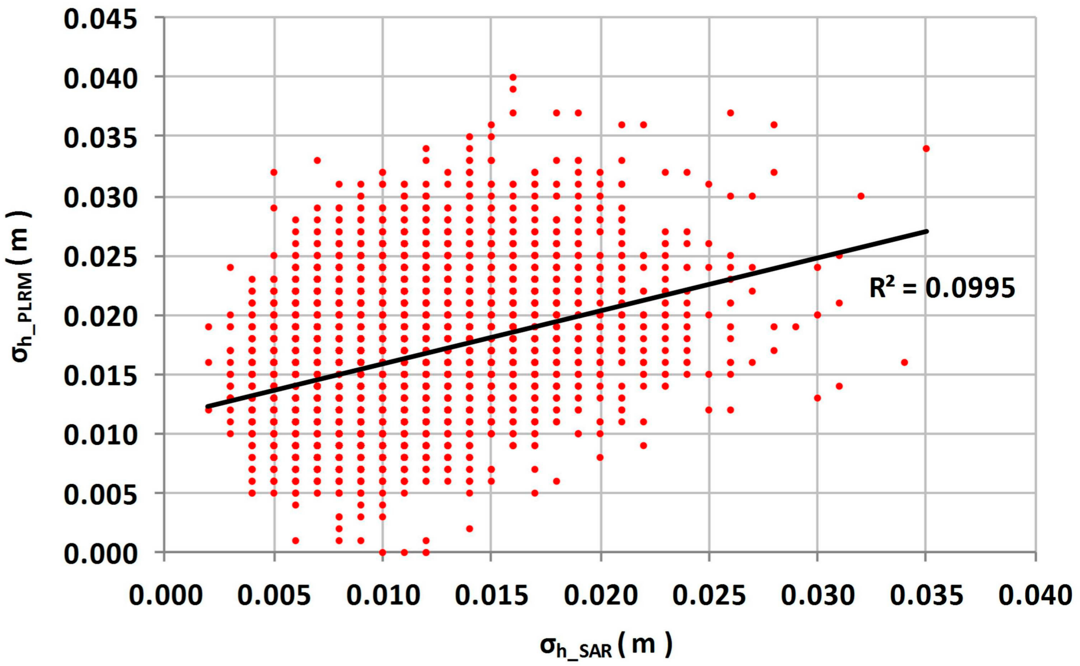
Furthermore, we investigated a possible correlation between the of the two altimeter products. Figure 4 shows that the two are uncorrelated (R2 = 0.09). Moreover, PLRM error was, on average, larger than SAR error: 0.0157 versus 0.0096. This agrees, at least qualitatively, with previous results that have provided a larger PLRM than SAR (see, for instance, Figure 1a in [7]).
Finally, we investigated the correlation between the of both altimeter products and various parameters of the sea states within the data set (see Figure 5 and Table 3).
The only relevant result was a modest—but non-negligible—correlation between the total significant wave height, SWHt, and the SAR 1 Hz standard deviation, (R2 = 0.4). On the contrary, there was no correlation between either of the two components of the sea spectrum (SWHs and SWHw) and SAR or PLRM (see Table 3).
Similar calculations, carried out on the average periods of the sea state components, show no relevant connection with either SAR or PLRM values (Table 4).
Multiple correlations between and SWHt and Tt yield the same results as the respective simple regressions between and SWHt, thus, confirming the lack of any simple correlation with the average wave period (Figure 6 and Table 5).
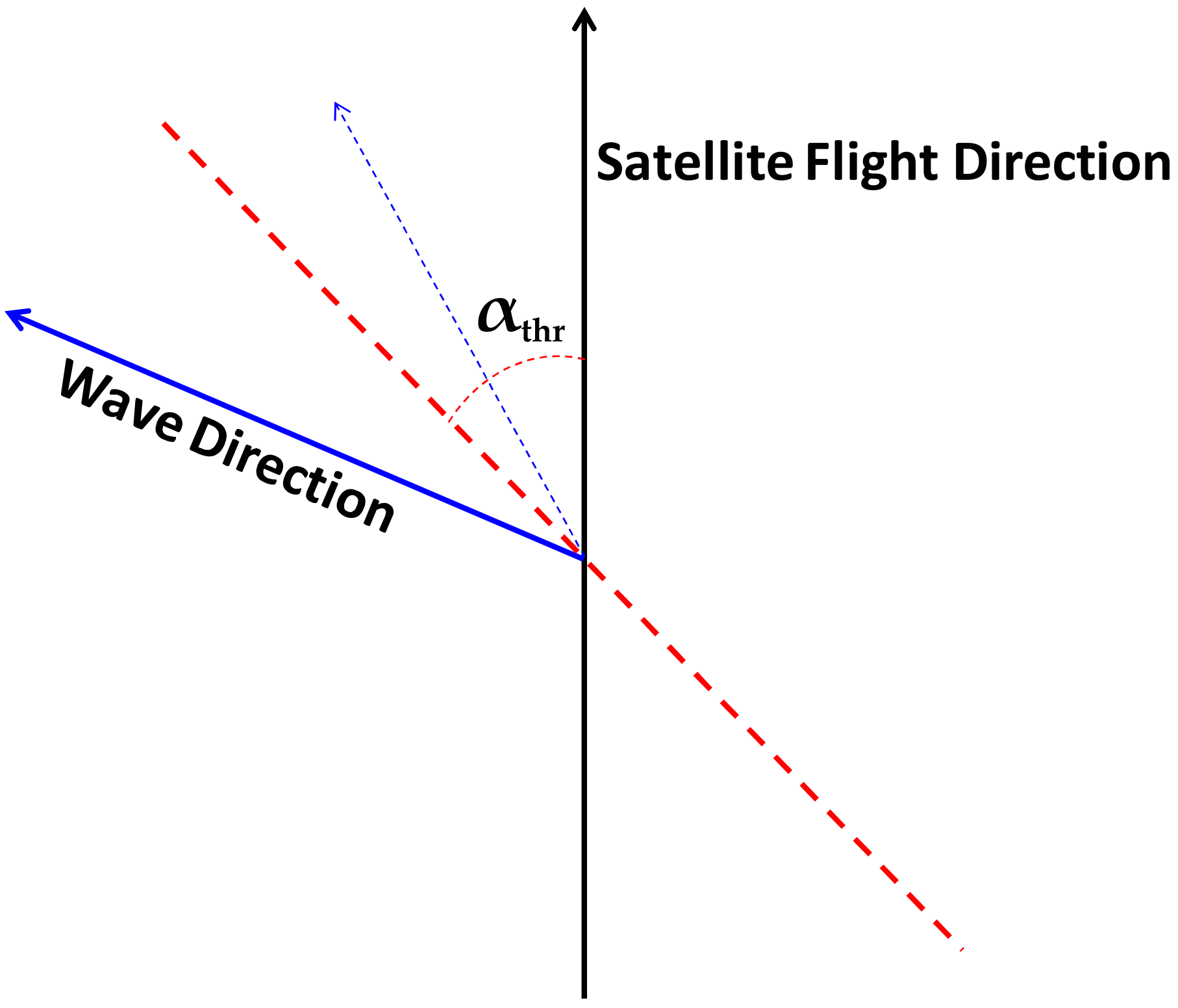
The direction of the wave system should also play a role, however, a simple correlation with the angle, α, between the average wave propagation and the satellite track would not produce any results, since any connection would be strongly non-linear. Therefore, a procedure has been tested to evaluate the influence of α. A threshold, αthr, was applied to the direction of the events considered: Only events where |α| > αthr were considered. See Figure 7.
For instance, if αthr is taken to be 40°, all sea directions whose propagation angle with the flight direction was less than 40° were excluded. The results are shown in Figure 8.
Again, the correlation between SWHt and was clearly higher for the SAR altimeter data, compared to the same correlation for the PLRM data, this latter being practically negligible (R2 = 0.15), while the former, independently from the threshold, was constantly about 0.40 except for a small decrease as αthr approached 90°: i.e., if only nearly perpendicular events are considered, the correlation decreases.
4. Discussion
We have shown that , as measured by DDA, had a non-negligible correlation with the total SWHt, while the correlation was much lower if only the swell component was considered. No such effect exists for the PLRM data considered here.
Furthermore, the relative direction between the wave system and the satellite path seems to bear little or no influence on the SAR behaviour.
While many physical effects may cause the altimeter SSH noise, the aliasing effect between the SAR altimeter resolution and the sea wavelength should play a role in the formation of .
A deeper insight can only be gained by numerically investigating the measuring procedure [19,20], thus, a simple conceptual numerical model of the Doppler altimeter (Figure 9) was implemented to evaluate the aliasing effect, which should contribute to the measured .
A bi-dimensional model was considered, with a fixed angle, α, between the satellite flight path and the wave direction. Spectral numerically simulated JONSWAP (Joint North Sea Wave Observation Project) wave trains, with a significant wave height (Hm), average wavelength period ™, and corresponding wavelength (Lm), were considered. Indeed, in real life, the waves are far from being sinusoidal: Each sea state is normally made up of a number of components of a spectrum. The surface was sampled at 20 Hz, i.e., 20 samples (looks) over a length of 6960 m. Thus, the distance between samples was 6960/20, which is 348 m, and was comparable to the along-track theoretical resolution of DDA. Therefore, we assume that the along-track altimeter resolution was equal to the sample length at 20 Hz. The error, , which can be assumed as a proxy of the part of the induced by the aliasing effect, was computed as the standard deviation of the simulated 20 Hz SSH:
where is the average SSH over sample i (348 m long) and is the average of over the one second interval (Equation (3)):
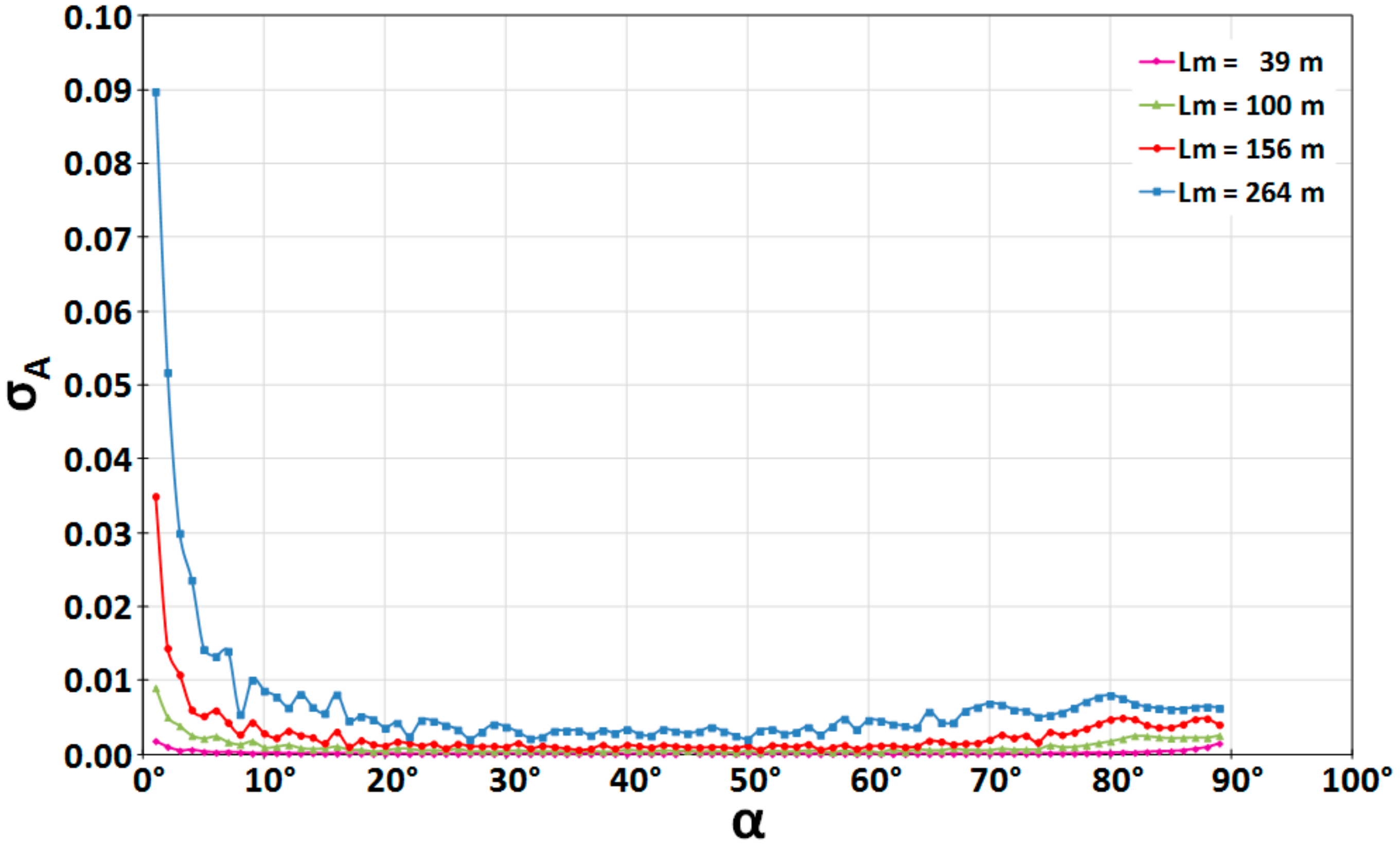
The aliasing effect can then be investigated by varying wave parameters, i.e., Hm and Lm, as well as the angle, α, between the satellite flight path and the wave direction. Figure 10 shows the dependence on α and Lm for a fixed wave height, Hm = 3 m.
There are some noteworthy conclusions to make on these results. First, and foremost, the aliasing effect was generally small, except for sea states very closely aligned with the satellite track; for most of the directions, was of the order of a few millimetres at most (compared with the average = 1.56 cm of the experimental DDA values as reported above) and it was basically independent of the angle, α. This result was derived from the use of a realistic spectrum rather than of a single sine wave, so little or no aliasing resonance takes place. It also appears that the length, Lm, did play a role, but even for the highest wavelength considered here (Lm = 264 m, Tm = 13 s) this was negligible. As it was shown above, very few of the events considered have an average wavelength, Lm, that was over 156 m (Tm = 10 s).
It should also be noted that sea states that happen to be strictly aligned with the track would show a relevant , comparable or even larger than . This is, however, a rare occurrence that did not appear in the experimental data: As shown above, very few—if any—of the sea states were aligned with the satellite directions.
5. Conclusions
A number of correlations have been carried out on German Bight CryoSat-2 SAR altimeter data to investigate the error of SSH as measured by SAR altimeter, in comparison with conventional simulated low resolution mode PLRM. Results show that, on average, PLRM error is larger than SAR error, confirming previous results and analyses [7].
We also found that the sea state SWH influenced the measurement of SSH for Delay Doppler Altimeter (DDA), introducing a 20 Hz error (), while it had no influence on PLRM data. DDA was slightly, but consistently, correlated with the significant wave height, but not to any wavelength parameter.
At least for the case examined, which only covered an area not exposed to the ocean, neither the presence of swell, nor the spectral average periods, were good indicators of SSH oscillation; in other words, wavelength does not seem to affect .
To verify these results, a bi-directional model of the aliasing curve—simulated alias-induced versus sea wavelength and direction—was implemented; it was proved that is generally very small in comparison with the error except for the direction aligned with the satellite paths. According to these results, the wave climate of the Northern sea—relatively short wind waves, directions that are generally not aligned with the satellite tracks—does not appear to induce any aliasing effect, and this accounts for the lack of correlation of SAR with the wavelength. It is possible, though, that investigations over open oceans might lead to different results.
Author Contributions
F.D. and L.F.-M. had the original ideas; F.R. carried out most of computations; E.P.C. and L.F.-M. coordinated the work.
Funding
Institutional funding from University of Salerno and University of Bonn.
Acknowledgments
Wave data from Meteorological Archival and Retrieval System (MARS) of ECMWF (European Centre for Medium-Range Weather Forecasts). Altimeter data from the ESA-ESRIN GPOD platform (https://gpod.eo.esa.int/). Technical support by ESA, through EO-Project 1172 “Remote Sensing of Wave Transformation” and by C.U.G.RI. (University Consortium for Research on Major Hazards—University of Naples and Salerno) is gratefully acknowledged.
Conflicts of Interest
The authors declare no conflict of interest.
References
- Jensen, J.R.; Raney, R.K. Delay/Doppler radar altimeter: Better measurement precision. In Proceedings of the IGARSS ’98: Sensing and Managing the Environment: 1998 IEEE International Geoscience and Remote Sensing Symposium, Seattle, WA, USA, 6–10 July 1998; Stein, T., Ed.; Institute of Electrical and Electronics Engineers, Inc.: Piscataway, NJ, USA, 1998. [Google Scholar]
- Raney, R.K. The Delay/Doppler Radar Altimeter. IEEE Trans. Geosci. Remote Sens. 1998, 36, 1578–1588. [Google Scholar] [CrossRef]
- Wingham, D.J.; Wallis, D.W. The Rough Surface Impulse Response of a Pulse-Limited Altimeter with an Elliptical Antenna Pattern. IEEE Antennas Wirel. Propag. Lett. 2010, 9, 232–235. [Google Scholar] [CrossRef]
- Benassai, G.; Migliaccio, M.; Montuori, A. Sea wave numerical simulations with COSMO-SkyMed© SAR data. J. Coast. Res. 2013, 1, 660–665. [Google Scholar] [CrossRef]
- Reale, F.; Dentale, F.; Carratelli, E.P. Numerical Simulation of Whitecaps and Foam Effects on Satellite Altimeter Response. Remote Sens. 2014, 6, 3681–3692. [Google Scholar] [CrossRef] [Green Version]
- Xu, Z.; Zhou, W.; Sun, Z.; Yang, Y.; Lin, J.; Wang, G.; Cao, W.; Yang, Q. Estimating the Augmented Reflectance Ratio of the Ocean Surface When Whitecaps Appear. Remote Sens. 2015, 7, 13606–13625. [Google Scholar] [CrossRef] [Green Version]
- Dibarboure, G.; Boy, F.; Desjonqueres, J.D.; Labroue, S.; Lasne, Y.; Picot, N.; Poisson, J.C.; Thibaut, P. Investigating Short-Wavelength Correlated Errors on Low-Resolution Mode Altimetry. J. Atmos. Ocean. Technol. 2014, 31, 1337–1362. [Google Scholar] [CrossRef]
- Peral, E.; Rodríguez, E.; Esteban-Fernández, D. Impact of Surface Waves on SWOT’s Projected Ocean Accuracy. Remote Sens. 2015, 7, 14509–14529. [Google Scholar] [CrossRef] [Green Version]
- Hwang, P.A.; Plant, W.J. An analysis of the effects of swell and surface roughness spectra on microwave backscatter from the ocean. J. Geophys. Res. 2010, 115. [Google Scholar] [CrossRef] [Green Version]
- Gommenginger, C.; Cipollini, P.; Snaith, H.; West, L.; Passaro, M. SAR altimetry over the open and coastal ocean: Status and Open issues. In Proceedings of the Ocean SAR Altimetry Expert Group Meeting, Southampton, UK, 26–27 June 2013; Available online: http://www.satoc.eu/projects/CP4O/docs/SARALT_EG_pdfs/cg1_CP4O_SARExpert_2627June2013.pdf (accessed on 15 February 2018).
- Gommenginger, C.; Martin-Puig, C.; Amarouche, L.; Raney, R.K. Review of State of Knowledge for SAR Altimetry over Ocean. Report of the EUMETSAT JASON-CS SAR Mode Error Budget Study; EUMETSAT Reference, EUM/RSP/REP/14/749304, Version 2.2; National Oceanography Centre: Southampton, UK, 2013; p. 57. [Google Scholar]
- Moreau, T.; Labroue, S.; Thibaut, P.; Amarouche, L.; Boy, F.; Picot, N. Sensitivity of SAR Mode Altimeter to Swell Effect. In Proceedings of the CryoSat Third User Workshop, Dresden, Germany, 12–14 March 2013; Ouwehand, L., Ed.; ESA Communications ESTEC: Noordwijk, The Netherlands, 2014. [Google Scholar]
- Garcia, E.S.; Sandwell, D.T.; Smith, W.H.F. Retracking CryoSat-2, Envisat and Jason-1 radar altimetry waveforms for improved gravity field recovery. Geophys. J. Int. 2014, 196, 1402–1422. [Google Scholar] [CrossRef] [Green Version]
- Galin, N.; Wingham, D.J.; Cullen, R.; Fornari, M.; Smith, W.H.F.; Abdalla, S. Calibration of the CryoSat-2 Interferometer and Measurement of Across-Track Ocean Slope. IEEE Trans. Geosci. Remote Sens. 2013, 51, 57–72. [Google Scholar] [CrossRef]
- Fenoglio-Marc, L.; Dinardo, S.; Scharroo, R.; Roland, A.; Dutour Sikiric, M.; Lucas, B.; Becker, M.; Benveniste, J.; Weiss, R. The German Bight: A validation of CryoSat-2 altimeter data in SAR mode. Adv. Space Res. 2015, 55, 2641–2656. [Google Scholar] [CrossRef]
- Dinardo, S.; Fenoglio-Marc, L.; Buchhaupt, C.; Becker, M.; Scharro, R.; Fernandes, M.J.; Benveniste, J. Coastal SAR and PLRM altimetry in German Bight and West Baltic Sea. Adv. Space Res. 2017. [Google Scholar] [CrossRef]
- Buchhaupt, C.; Fenoglio-Marc, L.; Dinardo, S.; Scharroo, R.; Becker, M. A fast convolution based waveform modell for conventional and unfocused SAR altimetry. Adv. Space Res. 2017. [Google Scholar] [CrossRef]
- Reale, F.; Dentale, F.; Carratelli, E.P.; Torrisi, L. Remote Sensing of Small-Scale Storm Variations in Coastal Seas. J. Coast. Res. 2014, 30, 130–141. [Google Scholar] [CrossRef]
- Carratelli, E.P.; Dentale, F.; Reale, F. Numerical Pseudo-Random Simulation of SAR Sea and Wind Response. In Proceedings of the Advances in SAR Oceanography from Envisat and ERS Missions (SEASAR 2006), Frascati, Italy, 23–26 January 2006; Lacoste, H., Ouwehand, L., Eds.; ESA Publications Division ESTEC: Noordwijk, The Netherlands, 2006. [Google Scholar]
- Montuori, A.; Ricchi, A.; Benassai, G.; Migliaccio, M. Sea Wave Numerical Simulations and Verification in Tyrrhenian Costal Area with X-Band Cosmo-Skymed SAR Data. In Proceedings of the ESA, SOLAS & EGU Joint Conference “Earth Observation for Ocean-Atmosphere Interactions Science”, Frascati, Italy, 29 November–2 December 2011; Ouwehand, L., Ed.; ESA Communications ESTEC: Noordwijk, The Netherlands, 2012. [Google Scholar]
Figure 1.
A map of the North Sea. Study area is delimited by the black box and is between 53–59° of latitude and 4–9° of longitude.
Figure 1.
A map of the North Sea. Study area is delimited by the black box and is between 53–59° of latitude and 4–9° of longitude.

Figure 2.
Distribution of events end event wave energy according to direction (a,c) and wavelength (b,d) for the whole spectrum (a,b) and the swell component (c,d). Dashed lines show the approximate satellite flight direction.
Figure 2.
Distribution of events end event wave energy according to direction (a,c) and wavelength (b,d) for the whole spectrum (a,b) and the swell component (c,d). Dashed lines show the approximate satellite flight direction.

Figure 3.
Altimeter versus ECMWF co-located SWH values: (a) Altimeter in SAR mode; and (b) altimeter in PLRM mode.
Figure 3.
Altimeter versus ECMWF co-located SWH values: (a) Altimeter in SAR mode; and (b) altimeter in PLRM mode.

Figure 4.
Correlation between the standard deviation, , of SSH in SAR and PLRM mode.

Figure 5.
Correlation between the standard deviation, , of SSH and SWHs, SWHw and SWHt: (a,c,e) altimeter in SAR mode; (b,d,f) altimeter in PLRM mode.
Figure 5.
Correlation between the standard deviation, , of SSH and SWHs, SWHw and SWHt: (a,c,e) altimeter in SAR mode; (b,d,f) altimeter in PLRM mode.

Figure 6.
Multiple correlation between , SWHt, and Tt both for the SAR (a) and PLRM data (b).

Figure 7.
Effect of wave direction: Only events that fall outside the threshold angle αthr are considered.
Figure 7.
Effect of wave direction: Only events that fall outside the threshold angle αthr are considered.

Figure 8.
Correlation coefficient between and SWHt as a function of the threshold angle, αthr.

Figure 9.
Schematic of the SAR altimeter conceptual model.

Figure 10.
Aliasing effect, , as a function of the angle, α, between the satellite flight path and the wave direction for four different average wavelengths, Lm, and for a fixed wave height, Hm = 3 m.
Figure 10.
Aliasing effect, , as a function of the angle, α, between the satellite flight path and the wave direction for four different average wavelengths, Lm, and for a fixed wave height, Hm = 3 m.


Table 1.
Repartition of sea state within all ECMWF dataset.
| Parameters | SWHt | SWHw | SWHs |
|---|---|---|---|
| ASWH (m) | 1.68 | 1.20 | 0.94 |
| SSSWH (m2) | 1.54 | 74,620 | 37,484 |
| En/Entot | 1.00 | 0.66 | 0.33 |
Table 2.
Average (A) and standard deviation (SD) of the three spectrum average wavelength components for the events in the ECMWF dataset.
Table 2.
Average (A) and standard deviation (SD) of the three spectrum average wavelength components for the events in the ECMWF dataset.
| Parameters | Lt | Lw | Ls |
|---|---|---|---|
| A (m) | 51.92 | 29.14 | 73.45 |
| SD (m) | 27.83 | 22.43 | 38.90 |
Table 3.
Correlation coefficients, R2, between values for the SAR and PLRM mode and the three SWH components of the wave spectrum.
Table 3.
Correlation coefficients, R2, between values for the SAR and PLRM mode and the three SWH components of the wave spectrum.
| Altimeter Mode | Swell (SWHs) | Wind (SWHw) | Total (SWHt) |
|---|---|---|---|
| SAR mode | 0.15 | 0.30 | 0.41 |
| PLRM mode | 0.07 | 0.12 | 0.11 |
Table 4.
Correlation coefficients, R2, between values for the SAR and PLRM mode and the mean periods of the wave spectrum and of its swell and wind components.
Table 4.
Correlation coefficients, R2, between values for the SAR and PLRM mode and the mean periods of the wave spectrum and of its swell and wind components.
| Altimeter Mode | Swell (Ts) | Wind (Tw) | Total (Tt) |
|---|---|---|---|
| SAR mode | 0.25 | 0.26 | 0.24 |
| PLRM mode | 0.11 | 0.12 | 0.11 |
Table 5.
Multiple correlation coefficients, R2, between values, SWHt, and Tt of the total spectrum for the SAR and PLRM data.
Table 5.
Multiple correlation coefficients, R2, between values, SWHt, and Tt of the total spectrum for the SAR and PLRM data.
| Altimeter Mode | Total (SWHt) |
|---|---|
| SAR mode | 0.41 |
| PLRM mode | 0.16 |
© 2018 by the authors. Licensee MDPI, Basel, Switzerland. This article is an open access article distributed under the terms and conditions of the Creative Commons Attribution (CC BY) license (http://creativecommons.org/licenses/by/4.0/).
Share and Cite
MDPI and ACS Style
Reale, F.; Dentale, F.; Carratelli, E.P.; Fenoglio-Marc, L. Influence of Sea State on Sea Surface Height Oscillation from Doppler Altimeter Measurements in the North Sea. Remote Sens. 2018, 10, 1100. https://doi.org/10.3390/rs10071100
AMA Style
Reale F, Dentale F, Carratelli EP, Fenoglio-Marc L. Influence of Sea State on Sea Surface Height Oscillation from Doppler Altimeter Measurements in the North Sea. Remote Sensing. 2018; 10(7):1100. https://doi.org/10.3390/rs10071100
Chicago/Turabian StyleReale, Ferdinando, Fabio Dentale, Eugenio Pugliese Carratelli, and Luciana Fenoglio-Marc. 2018. "Influence of Sea State on Sea Surface Height Oscillation from Doppler Altimeter Measurements in the North Sea" Remote Sensing 10, no. 7: 1100. https://doi.org/10.3390/rs10071100
Note that from the first issue of 2016, this journal uses article numbers instead of page numbers. See further details here.