Article

Detecting Vegetation Change in Response to Confining Elephants in Forests Using MODIS Time-Series and BFAST

1
School of Science and Engineering, Manchester Metropolitan University, Chester Street, Manchester M1 5GD, UK
2
Chester Zoo, Cedar House, Caughall Road, Upton by Chester, Chester CH2 1LH, UK
3
Kenya Wildlife Service, P.O. Box 40241-00100, Nairobi 00100, Kenya
*
Author to whom correspondence should be addressed.
Remote Sens. 2018, 10(7), 1075; https://doi.org/10.3390/rs10071075
Submission received: 4 June 2018 / Revised: 3 July 2018 / Accepted: 4 July 2018 / Published: 6 July 2018
(This article belongs to the Special Issue GIS and Remote Sensing advances in Land Change Science)

Abstract

:
Afromontane forests are biodiversity hotspots and provide essential ecosystem services. However, they are under pressure as a result of an expanding human population and the impact of climate change. In many instances electric fencing has become a necessary management strategy to protect forest integrity and reduce human-wildlife conflict. The impact of confining hitherto migratory elephant populations within forests remains unknown, and monitoring largely inaccessible areas is challenging. We explore the application of remote sensing to monitor the impact of confinement, employing the Breaks For Additive Season and Trend (BFAST) time-series decomposition method over a 15-year period on Moderate Resolution Imaging Spectroradiometer (MODIS) Enhanced Vegetation Index (EVI) (MOD13Q1) datasets for two Kenyan forests. Results indicated that BFAST was able to identify disturbances from anthropogenic, fire and elephant damage. Sequential monitoring enabled the detection of gradual changes in the forest canopy, with degradation and regeneration being observed in both sites. Annual rates of forest loss in both areas were significantly lower than reported in other studies on Afromontane forests, suggesting that installing fences has reduced land-use conversion from human-related disturbances. Negative changes in EVI were predominantly gradual degradation rather than large-scale, abrupt clearings of the forest. Results presented here demonstrate that BFAST can be used to monitor biotic and abiotic drivers of change in Afromontane forests.

Graphical Abstract

1. Introduction

Over 31% of the Earths’ surface is covered by forests, and maintaining the integrity of forest ecosystems is a global conservation concern [1]. The East African montane forests, rich in biodiversity and providers of vital ecosystem services to the human population, are under intense pressure [2,3,4]. Although there is no consensus on the impact of climate change on lowland productivity [5,6], analysis suggests that some areas have become drier, noticeably reducing the length of the growing season [6]. The combination of rising temperatures and altered rainfall patterns is a major factor in food insecurity [7,8,9]. Subsequently, with increasing human populations and a decline in productivity in the rangelands, pressure on the East African montane ecosystems is expected to increase.
Montane forests and highland areas account for 15.2% of Kenya‘s total area [1]. Five of these, namely the Aberdare National Park (ANP), Mount Kenya, Mau Complex, Cherangani Hills and Mount Elgon, are known as the “Water Towers”; they are an important water resource for the country [4], accounting for 75% of the renewable surface water [10]. Two of these “Water Towers” (Aberdare mountain range and Mount Kenya) produce 55% of Kenya’s electricity, which is generated by hydropower, and support major irrigation schemes required by the agricultural sector that contributes to a quarter of the country’s GDP [11]. The degradation of Kenya’s forests and subsequent impact on climate change could severely affect agricultural production [12,13] and lead to negative ramifications for the human population.
The Kenyan montane forests are refuges that became isolated during glacial maxima and recurrent expansions and contractions of the forest [14]. This history has produced centers of endemism and biodiversity hotspots which incorporate an extensive range of habitats promoting a unique biodiversity for East Africa [10,14]. They support a number of threatened mammal species, such as the critically endangered mountain bongo (Ragelaphus eurycerus), and are an internationally recognised Important Bird Areas. Although not a montane forest, or part of the “water towers” of Kenya, the Shimba Hills forest in the Southern coastal zone is a significant regional water catchment that is also monitored by various state agencies in charge of water towers. It contains three threatened and two restricted-range bird species, and is home to the country’s only population of sable antelope (Hippotragus niger) [15].
The areas surrounding Kenya’s forests have experienced large-scale changes in land-use as a result of a rapidly expanding human population, which has also led to an increasing competition for resources between people and wildlife. Human-elephant conflict (HEC) has become a major conservation concern [16] with increasing cases of property damage, crop raiding and human death and injury [17]. In response to HEC, and to protect the forests from the pressures of illegal activities, including logging, poaching and illegal kilns to supply the charcoal trade, Kenya has embarked on a strategy of using electric fencing enclosing the montane regions and other forests containing elephant populations. Although fencing some of the “Water Towers” and Shimba Hills National Reserve is already well underway, the impact of confined elephants on forest health, and the ramifications on other taxa that rely on these areas as dry season refugia, is unknown.
Under the threat of degradation by anthropogenic and biogenic pressures, and the little understood impact of fencing, it is becoming increasingly common to separate people and wildlife. There is an obvious need to assess the impact of fencing on the integrity of forest ecosystems and to monitor the long term health of forests to guide management strategies to preserve both species, and habitats. Previous techniques assessing the impact of mega-herbivores on ecosystems have been limited to the collection of ground data assessing tree damage [18,19,20]. A major drawback with this approach is that it is limited to only those areas that are relatively easily accessible and can only be conducted on a relatively small scale. Consequently, montane regions have remained relatively understudied as they are commonly found in largely inaccessible areas, with challenging terrain and limited road access [21,22].
With increasing habitat fragmentation from fencing and land use change, ecologists have become increasingly interested in the capacity of some species to permanently alter their habitat and modify the environment [23,24]. Elephants have been documented to reduce the cover of woodland [25] and cause large- and small-scale disturbances to the land. Bark-stripping, uprooting trees, and opening up vegetation by trampling plant communities whilst foraging, combined with their preferential seasonal feeding, can cause irreversible damage to trees and bushes [26]. In addition, they dig wells to reach water under the surface, and smooth rock surfaces and tree stumps whilst rubbing up against them to scratch [18,26,27]. In instances where there have been significant impacts, wildlife corridors and translocations of elephants have been used as a measure to limit and reverse such damage. In 2005, for example, as a response to elephant overpopulation, negative impacts on the vegetation [17], and to reduce HEC, 150 elephants were translocated from the Shimba Hills forest to Tsavo East National Park [28].
Over the last decade, there has been an increase in the use of remote sensing approaches for monitoring deforestation over large areas, due to the opening of the Landsat archive in 2008 [29,30,31]. The use of Earth observation (EO) data with challenging terrain is undoubtedly faster and more cost effective than approaches employing field data only [32].
Mapping changes in forest cover with remotely sensed imagery has most frequently been carried out using a bi-temporal change detection approach, whereby multiple images are selected from key points in time and land cover change maps are produced using a supervised classification technique (e.g., Maximum Likelihood, Random Forests) [33,34]. However, DeVries et al. [22] highlighted the potential problem of cloud contamination using this method, particularly when working in the tropics or in montane regions [35,36]. When using only a limited number of images during temporal comparisons, subtle disturbances and vegetation regrowth processes might be missed due to large temporal gaps in the period between start and end dates. This can be problematic when detailed vegetation dynamics are required to guide habitat management decision-making [37,38]. To avoid errors in change detection, it is also vital to select scenes that are from the same phenological period as seasonal variability within the forest can result in confusion between forest and non-forest pixels [22,33]. The sparse Landsat archive in large parts of East Africa further complicates the ability to choose appropriate imagery at this scale and for this region. As a result, LiDAR (Light Detection and Ranging) data is increasingly being used to map gaps in the forest canopy and to identify degradation [39,40]. However, persistent cloud cover, steep topography, limited temporal datasets and the high associated economic costs especially in developing areas means that LiDAR can be unsuitable for detecting change over time, particularly in montane forests [36].
To increase the sensitivity of detecting discrete changes in montane forest ecosystems, it is, therefore, advantageous to employ more robust approaches of dense time series analysis that can also consider seasonality [37,38,41,42,43]. The recent development of a range of algorithms including LandTrendR [44] for the Landsat archive and Breaks For Additive Season and Trend (BFAST) [21] for Landsat and Moderate Resolution Imaging Spectroradiometer (MODIS) datasets, has enabled near real time monitoring in the health and dynamics of ecosystems worldwide [38]. BFAST has previously been applied on a Landsat time-series using the Normalized Difference Vegetation Index (NDVI) in a montane forest in Ethiopia. It successfully identified small-scale forest disturbances, events characterised by a small number of pixels with varying magnitudes of change, from discrete clearings of the forest to progressive reductions in the canopy cover [22]. It has been proven to be robust in determining both discrete and abrupt changes in forest cover in a variety of habitats [42,45,46], even in regions with high cloud contamination, such as the Kenyan montane forests. Landsat data with a relatively fine spatial resolution (30 m-pixels), spanning more than four decades, could be ideal for studying forest disturbances using LandTrendR or BFAST. However, significant gaps in the archive exist over East Africa for the mid-1990s and early 2000s. The number of available Landsat scenes for the study sites at the time of analysis, and the significant gaps are shown in Appendix A. A trade-off in the spatial dimension, as well as the depth of the historical records, is to use imagery from MODIS at a very fine temporal (16-day) but coarser spatial (250 m pixel) resolution, to detect forest disturbances in this region [46,47,48].
Within this context, our aim was to detect vegetation change and assess forest condition in two fenced forests of Kenya. Both climatic and non-climatic drivers of change were considered, along with the impact of fencing elephants in forests, which has never been examined using dense time series analysis techniques with remote sensing data before. We employ BFAST on the Enhanced Vegetation Index (EVI) derived from MODIS time-series data in combination with Tropical Applications of Meteorology using SATellite (TAMSAT) monthly rainfall estimates and the MODIS burned area product to identify the direction and magnitude of change in the forest canopy. We also map the potential drivers of change, in combination with ground truth data, to assess the suitability of using medium-resolution satellite imagery providing near real-time information on the dynamics of Afromontane forests characterised by gradual change.

2. Materials and Methods

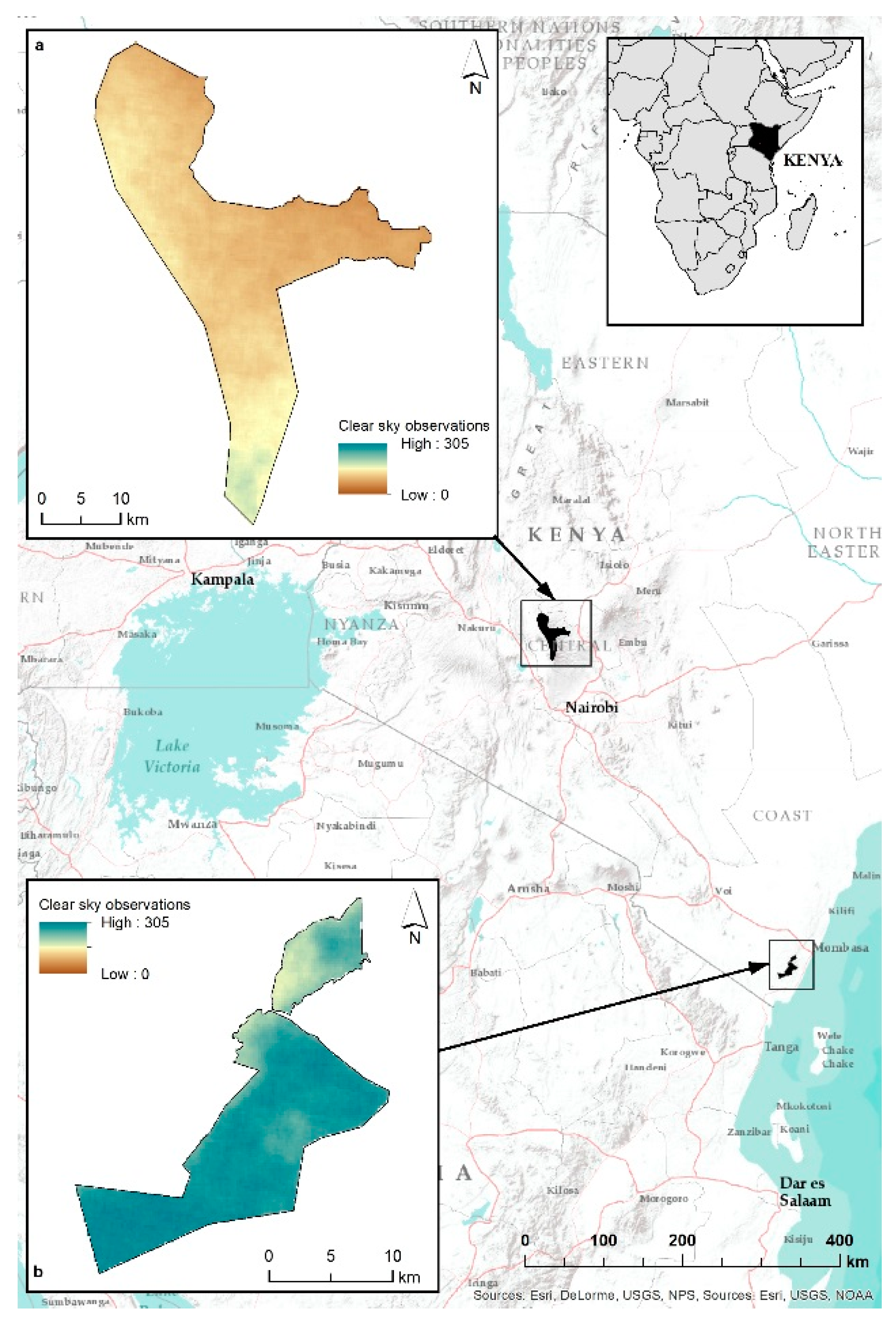
2.1. Study Site—Aberdare National Park, Kenya

The Aberdare National Park (ANP) covers an area of 766 km2 in the Central Province of Kenya. It lies southwest of Mount Kenya forming the Eastern rim of the Great Rift Valley (Figure 1). The altitude in the park varies from ~1800 m to ~4000 m. This high altitude means that the area experiences cloud cover throughout the majority of the year. Data extracted from the WorldClim database shows it has a uniform climate, with temperatures averaging 17 °C, and receiving approximately 1600 mm per annum. There are two ‘wet’ seasons, with the long rains starting in March and lasting until late May, and the short rains arriving in October and ending in December. In 1989, the construction of the world’s largest electric ‘wildlife’ fence surrounding the perimeter began. It was commissioned in eight phases and was completed in 2009 [11]. The area now contains a confined elephant population with a recent survey estimating ~4000 elephants (pers.com. Kenya Wildlife Service, 2017).

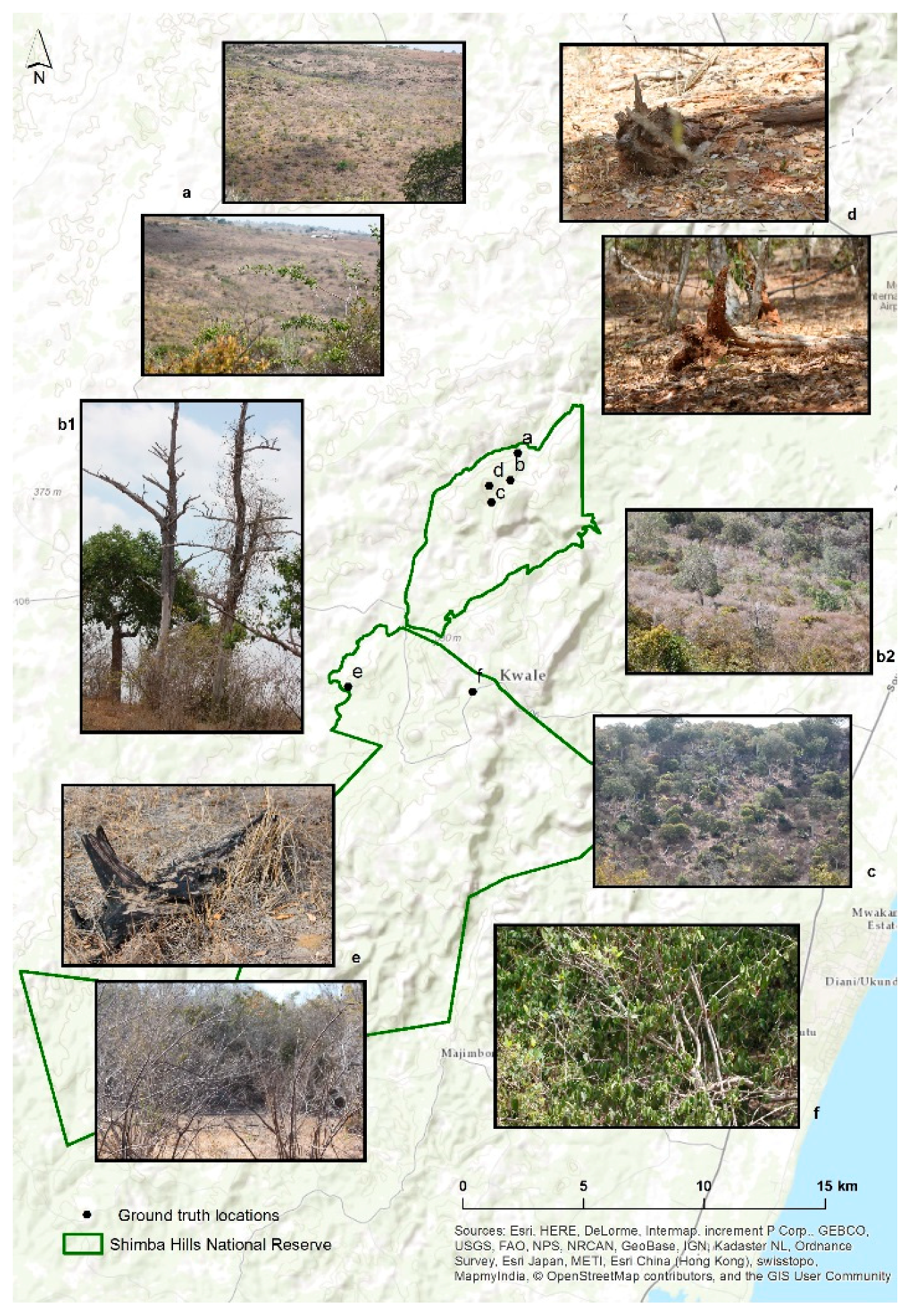
2.2. Study Site—Shimba Hills National Reserve, Kenya

Shimba Hills National Reserve (SHNR) is a smaller forest reserve covering 300 km2 located in the Kwale District in the Coastal Province of Kenya (Figure 1). The altitude within this Reserve is much lower than the ANP, averaging at just 348 m above sea level, meaning that the cloud cover across the area is significantly lower. WorldClim data gives temperatures averaging 25 °C, the area receives less rain than the ANP, averaging just 1162 mm per annum. This coastal region experiences two ‘rainy’ seasons. The highest volume of rain occurs between April and July, with shorter rains arriving in October and lasting until November. The perimeter has been fenced since 1999, with the current estimated elephant population in the reserve of >600 individuals. It is suggested that the elephant population is three times the recommended carrying capacity of circa 200 individuals [17].

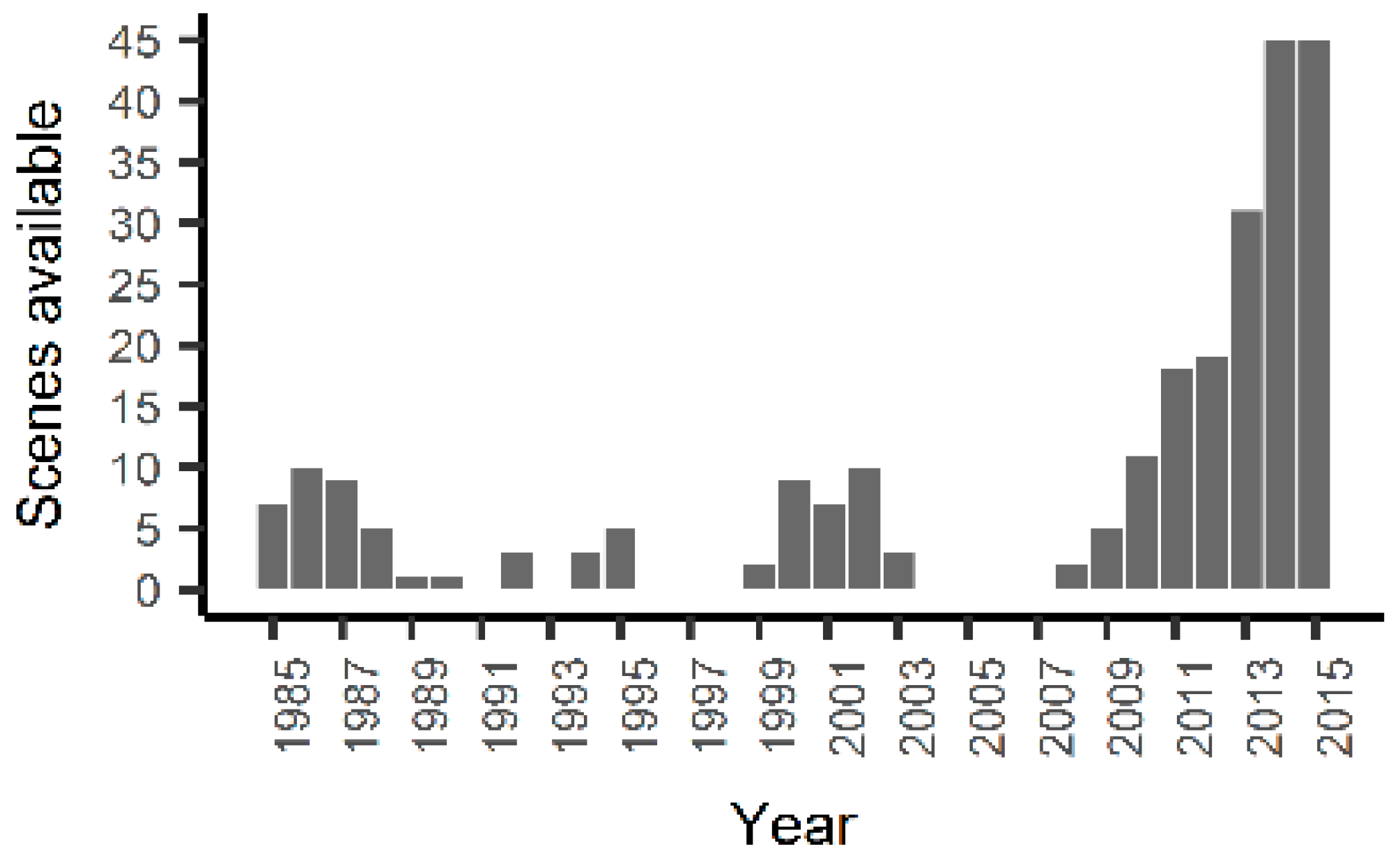
2.3. Satellite-Based Data
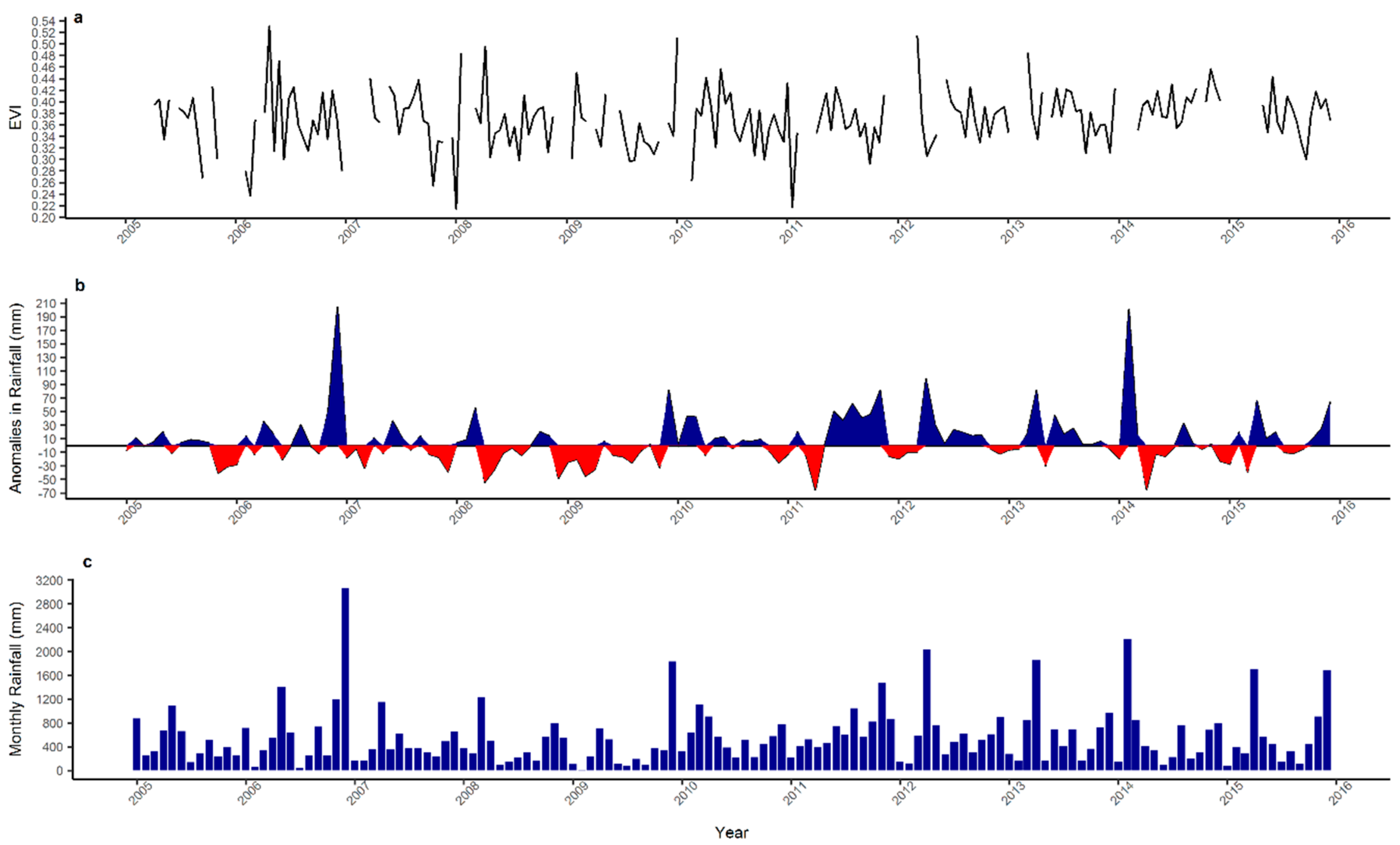
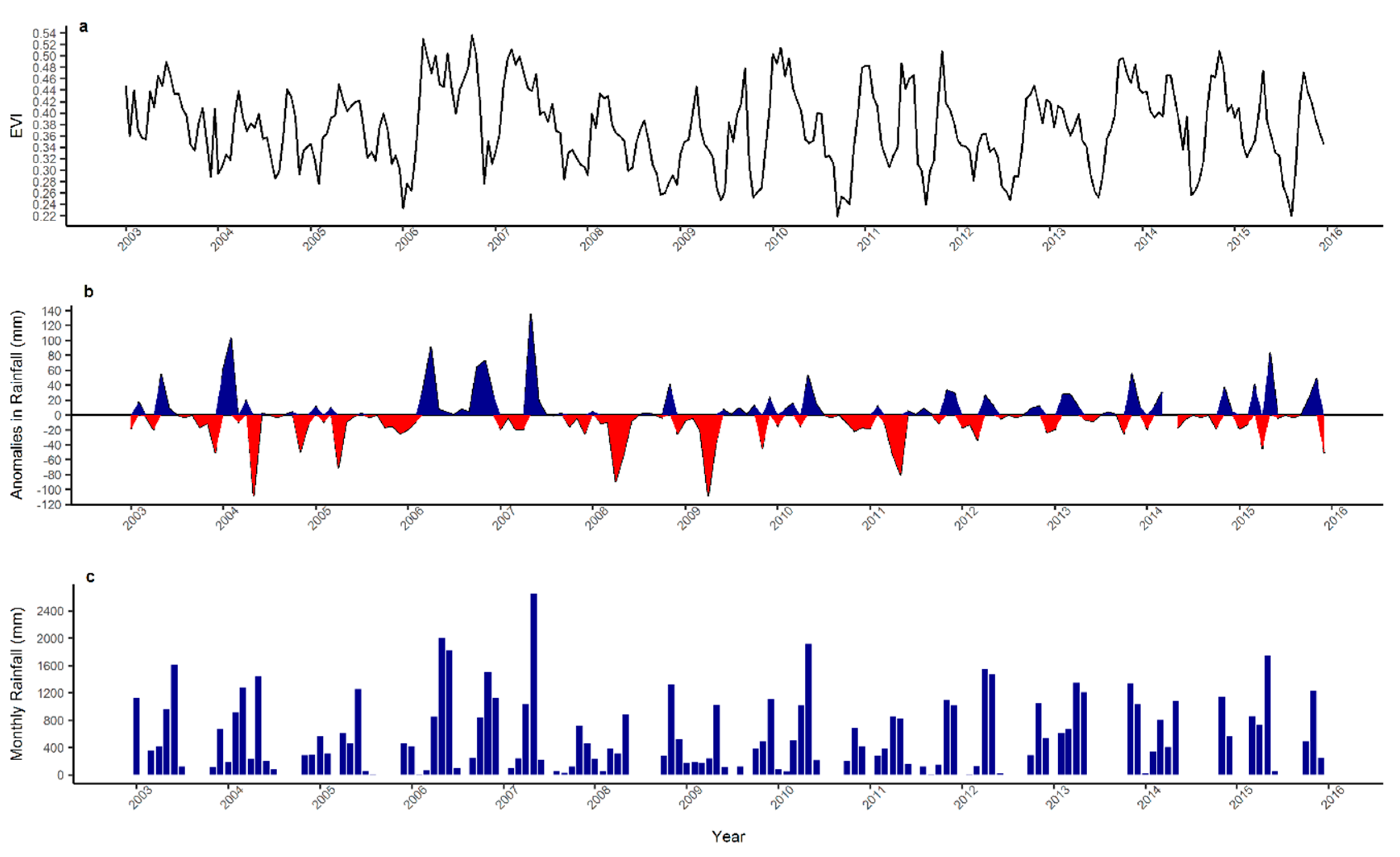
2.3.1. MODIS EVI

The response variable used to detect vegetation change was the MODIS Enhanced Vegetation Index (EVI), a measurement of photosynthetic activity in vegetation at a location, ranging from 0 (indicating no vegetation) to 1 (dense vegetation):
EVI = G NIR Red NIR + C 1 Red C 2 Blue + L
where G is the gain factor, NIR is the Near Infra-red band, C1 and C2 are the coefficients of the aerosol resistance term, and L is the canopy background. Whilst the Normalized Difference Vegetation Index (NDVI) [49] is commonly used [22,45], as in a number of other forest studies, we chose the EVI, [50,51,52] due to its improved performance in areas of high biomass as a result of a de-coupling of canopy background signals and a reduction in atmospheric influences [53]. We used the MODIS EVI product MOD13Q1 at 250 m spatial and a 16-day temporal resolution downloaded from the United States Geological Survey (USGS; Table 1).
All available scenes, totalling 386, an average of 23 per year, were acquired for each site spanning the period of February 2000 to December 2015, to produce 15-year annual profiles. The MOD13Q1 is provided as a surface reflectance product and masked for water, clouds, heavy aerosols, and cloud shadows. We applied another mask to the data in R [54] which employs the quality assessment layer, thus addressing pixel reliability. We only kept those pixels in the time-series analysis that were confidently ranked as of ‘good quality’ in the product information guide.

2.3.2. TAMSAT Rainfall

Monthly rainfall was also incorporated into the analysis to evaluate the effect of rainfall on the variation of the EVI values (Table 1). We employed the Tropical Applications of Meteorology Using Satellite and Ground-Based Observations (TAMSAT) monthly data with a 4 km spatial resolution [55,56,57]. The TAMSAT method calibrates the algorithm using rain gauge observations combined with contemporaneous cold-cloud duration (CCD) to infer rainfall estimates and anomalies [56]. We derived anomalies in rainfall patterns based on differences between the observed and expected volume of rainfall for each study site by running the BFAST algorithm on the monthly rainfall estimates data, to allow a visual representation.

2.3.3. MODIS Burned Area

To identify vegetation disturbance as a result of fire, the MODIS monthly MCD451A burned area product at 500 m spatial resolution was used to assess the timing and extent of burnt areas within the study sites (Table 1). The algorithm locates rapid changes by analysing the daily surface reflectance changes to identify recent fires. We downloaded data from the USGS archives and kept only the ‘use with confidence’ pixels (as labelled in the quality assessment layer provided with the dataset).

2.4. BFAST Method

To detect breakpoints in the MODIS EVI time series, we employed the BFAST approach [21] using the ‘bfastSpatial’ package [42,58,59]. Annual vegetation phenology follows a somewhat predictable cycle, with “greening” during the wet season and “browning” throughout the dry. Both seasonality and environmental factors including precipitation and temperature can cause variation in EVI values, particularly in non-forest areas, such as shrubland. The BFAST method breaks-down the time series into trend, season and residual components [21]. Fitting a seasonal trend accounts for these temporal fluctuations. Despite our focus being on detecting change in areas of primary forest, it was not possible to exclude non-forest pixels due to the absence of detailed land cover maps throughout the study period [60].
There are three stages in classifying change in the time-series using BFAST: (1) fitting a model based on pixel values from a stable history period; (2) testing observations in a time period following the history period in order to detect any deviations from the model; and (3) calculating the magnitude of change by examining the median residuals between the observed and expected value.

BFAST Parameters

Model for the additive seasonal trend: The “harmonic” model, used by Verbesselt et al. [41] to detect forest change, was considered to be the most suitable for phenological change detection of natural vegetation:
y t = α + ƴ sin ( 2 π t f + δ ) + ε t
where, yt and t are the response variable and time, f is the temporal frequency, α is the intercept, y and δ are the amplitude and phase of the harmonic component and εt is the residual (noise component) [22].
The factor h: h is the minimal segment size between potentially detected breaks in the trend model given as fraction relative to the sample size (i.e., the minimal number of observations in each segment divided by the total length of the timeseries). Given our sample size, we fixed the value of h at 0.1 in order for at least one complete phenological cycle between two break-points.
Stable history period: for the Aberdare National Park this was defined as the period between 2000 and 2004. Throughout this period, over 60% of the area remained un-fenced and the elephant population was able to follow former migration routes to the lowlands during the wet season. It was assumed that the pixels within the forest were relatively stable. For Shimba Hills National Reserve, we used a shorter stable history period from 2000 to 2002 as we were informed by Kenya Wildlife Service (KWS) that the northern part of the park within the Mwalunganje elephant sanctuary experienced large areas of degradation as a result of elephant damage after this period. A minimum of two years of stable history period was used as it is recommended that at least two years is required to accurately monitor change when employing the MODIS 16-day product [21].
Sequential monitoring: We used a sequential approach and limited the monitoring period to one-year consecutive periods in order to track gradual, incremental changes over time, as highlighted in previous BFAST applications [22]. Using a sequential method reduces the large number of observations post change detection and limits the impact this can have on the results of the change magnitude [22,43,45].

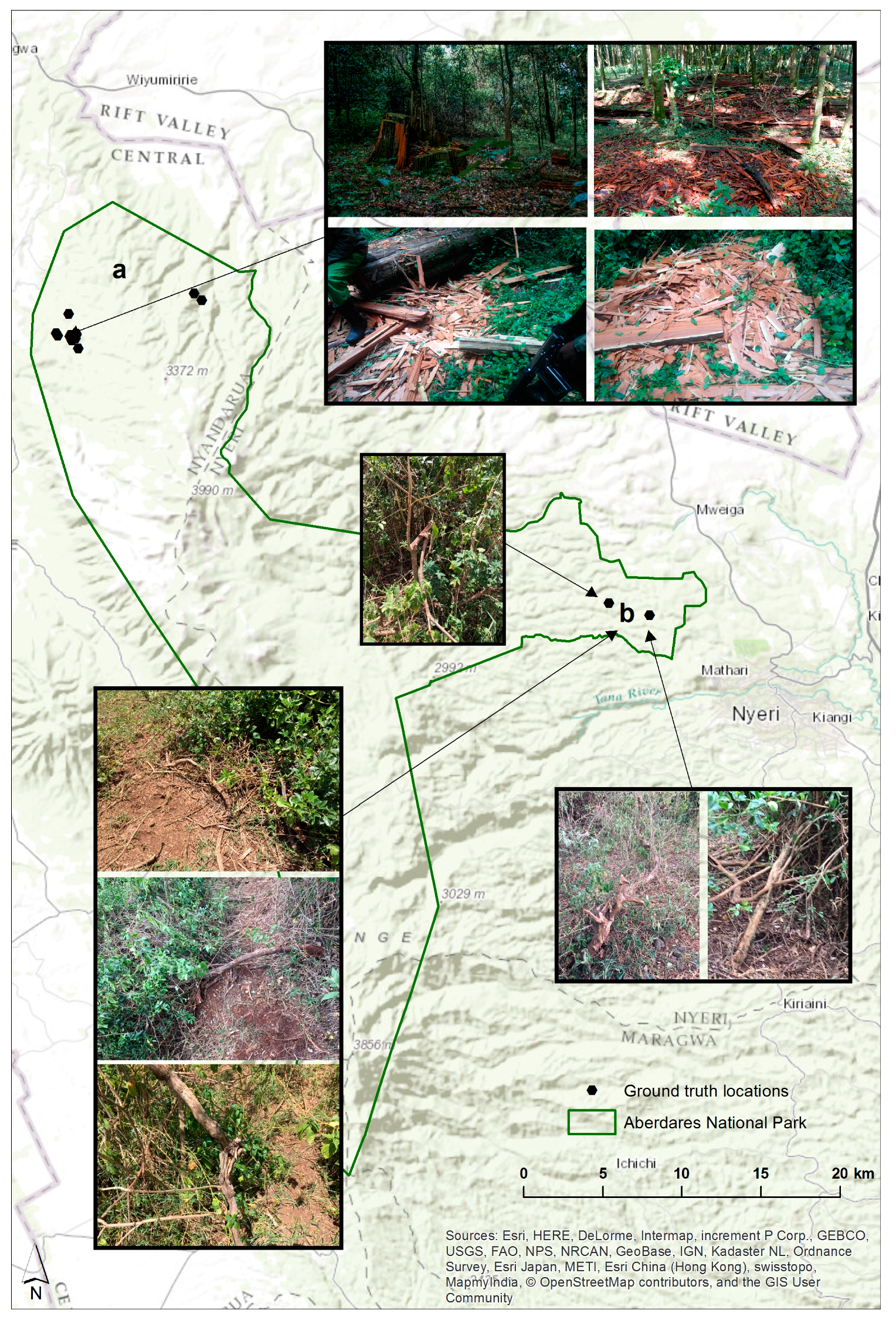
2.5. BFAST Validation
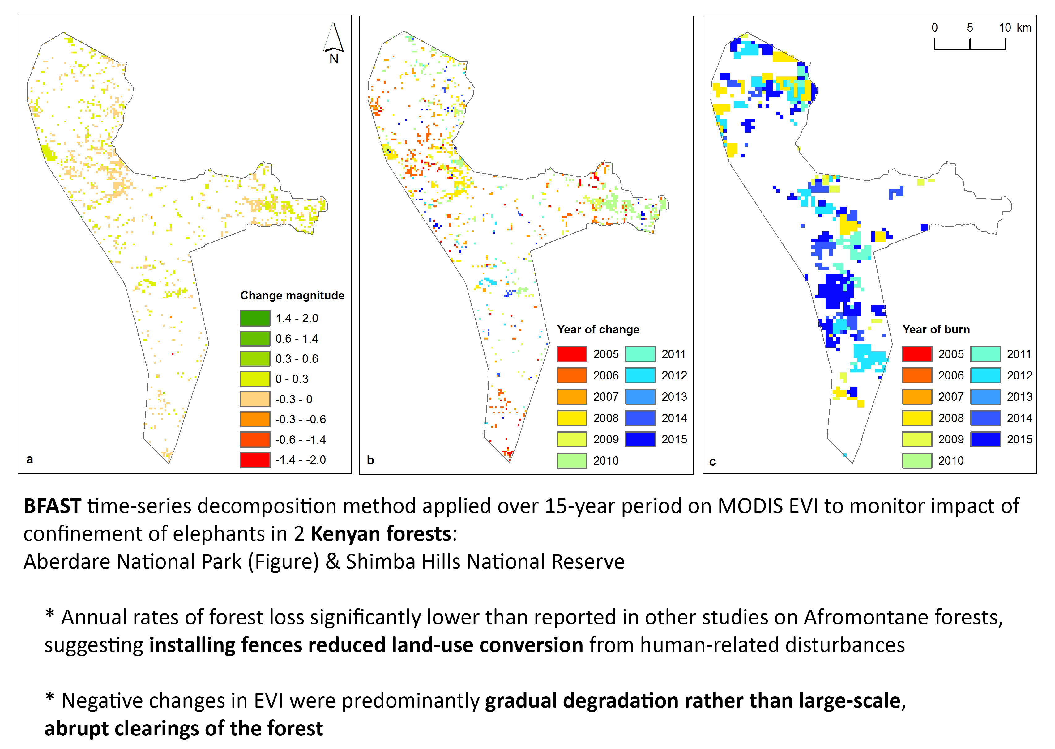
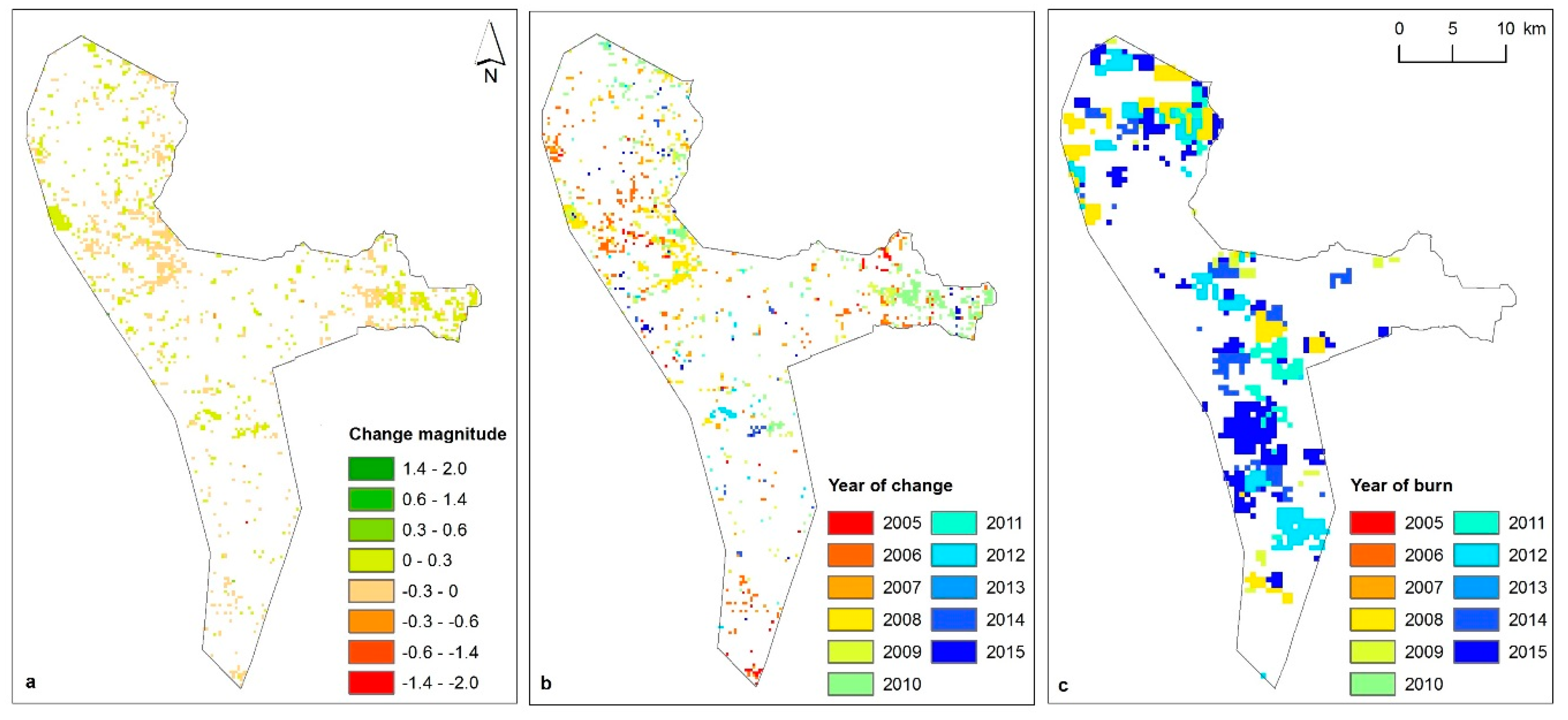
In order to assess the ability of a MODIS-based BFAST approach to detect disturbances in Afromontane forests caused by different drivers (e.g., anthropogenic, climatic, elephant damage), we randomly selected 495 forest and non-forest pixels across both study sites: 227 in the ANP and 268 in SHNR, separated into two strata (change detected and no change detected). Some studies use finer resolution Satellite Pour l’Observation de la Terre (SPOT), RapidEye, or Landsat data [22]. However, due to the large temporal gaps in the Landsat archive (Appendix A) over East Africa, and the failure of the scan-line corrector (SLC) on Landsat 7, we used the EVI profiles from the time-series using the BFAST monitor function within the ‘bfastspatial package’. We performed a visual interpretation comparable to TimeSync [61], at the pixel level, of an agreement or disagreement of a breakpoint or non-breakpoint pixel based on the validity of the model fitted and the trend of the EVI values for each pixel. Commission errors were recorded if there was disagreement when the model had incorrectly classified a breakpoint as a result of excessive noise within the data, or an unsuitable model fitted based on the stable history period. Omission errors were reported if the model did not correctly identify a breakpoint.
To further assess BFAST’s ability to identify changes, we carried out field visits during 2015 and 2016 and collected geolocated photographs from locations within our study areas were BFAST was able to identify disturbances in those years. Ideally, it would have been preferable to use very high resolution (VHR) imagery, such as aerial photos, for the duration of the study. However, these were not available for our study areas.

3. Results

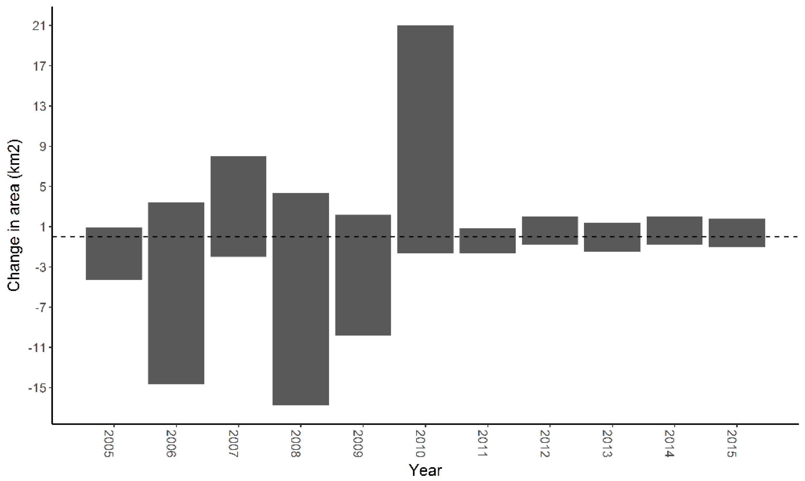
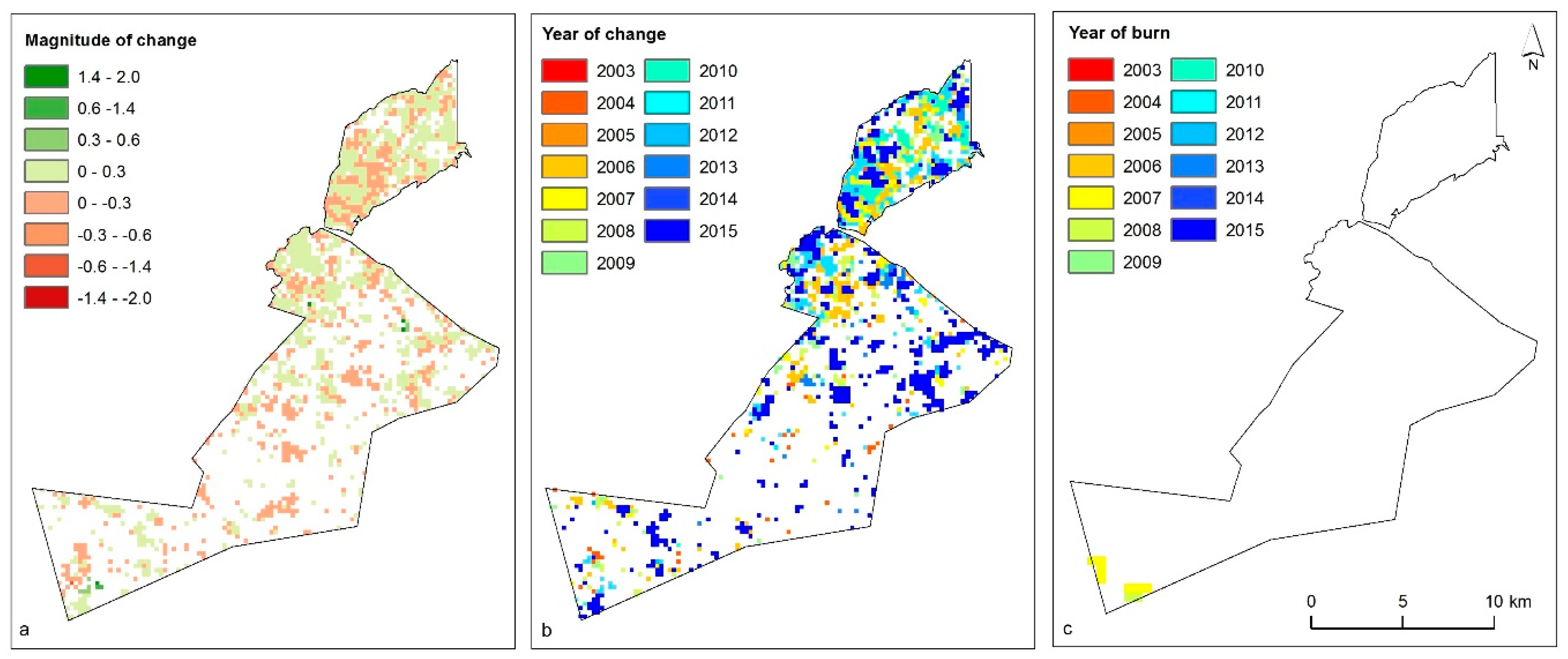
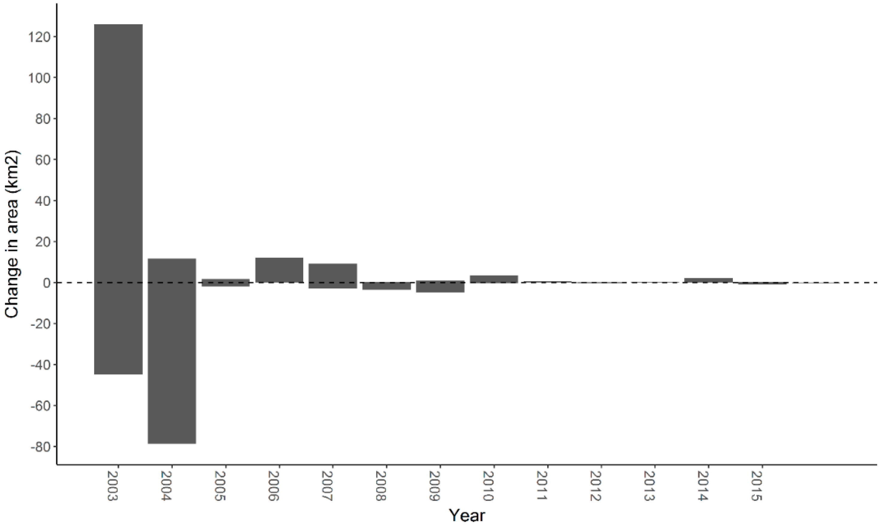
3.1. Aberdare National Park

The change maps produced using BFAST on the MODIS EVI data for the Aberdare National Park are shown in Figure 2, together with the year of change and years of burn data based on the MCD45A MODIS data.
Throughout the monitoring period, the ANP experienced 102.9 km2 of change in the vegetation cover as a result of climatic and non-climatic drivers. This represents approximately 13% of the Park. However, only 8 km2 represents negative change in the EVI values, therefore only 0.9% of loss to the parks vegetation occurred over the 11-year monitoring period; this corresponds to an annual rate of 0.09%. The direction of change indicates areas of negative change followed by regrowth. Ground truth visits suggest that certain areas of the Park are more susceptible to human influences. In northern parts of the Park we found evidence of both recent and old logging sites, and charcoal kilns. In central and eastern areas of the park, we found no evidence of tree stumps that had been “clean cut”, which is indicative of anthropogenic disturbance; only vegetation damaged by elephants was found (Figure 3).
Whilst data from the MODIS burned area product correlated well with some of the disturbances, there was a large number of disturbances identified by BFAST in locations that are not affected by fire, according to the MODIS product (Figure 2). Areas of disturbance that are not correlated with rainfall anomalies, anthropogenic disturbance or fire are potentially the result of damage caused by elephants, as found during ground truth visits (Figure 3). The most substantial disturbance in vegetation dynamics was 66.4 km2 between the years of 2005 and 2009, which was predominantly a negative trend (Figure 4).
The temporal profiles of MODIS EVI, rainfall anomalies and monthly rainfall estimates from TAMSAT are presented in Figure 5. Negative anomalies in rainfall were experienced in 2007; however, only 2 km2 ha of negative change in EVI occurred that year. In 2008, the year succeeding the negative trend in rainfall, small negative changes in the EVI values, with a magnitude of up to 0.2, where found (Figure 2a,b). Overall, negative anomalies in rainfall in the TAMSAT time series dominated the year 2009. Some 98.1 km2 of the park showed a decrease in EVI, with breakpoints at discrete magnitudes of 0.1–0.3 (Figure 2a,b). However, 0.4 km2 showed negative breakpoint magnitudes of 0.6–1.4 (Figure 2a), suggesting a small-scale, abrupt change, such as forest clearing. After a year of negative rainfall anomalies, the following year, 2010, reported higher-than-normal rains throughout the year, which coincided with 21 km2 of the park undergoing positive changes in EVI (Figure 4).

3.2. Shimba Hills National Reserve

The change maps produced for Shimba Hills National Reserve are shown in Figure 6. Over 306.8 km2 were found to have undergone significant change over the 12-year period, averaging a 9% of change in the reserve’s area per year. As in the case of the Aberdare National Park, this change is bi-directional with disturbance detected followed by regrowth identified as subsequent breakpoints in the following years. The majority of change occurred between the years 2003 and 2004. Removing these ‘outlier’ years from the analysis reduces the annual rate of change to 1.6%. Overall, approximately 11% of the reserve underwent an improvement with a significant greening of 54% between 2003 and 2004 (Figure 7).
Significant gaps in the MODIS burned area data over the SHNR (Figure 6c) meant that the product could not accurately detect burnt areas. We verified this during our ground truth data collection, as we were able to locate a number of areas with clear evidence of fire that the MODIS product had not been able to identify (Figure 8). This discrepancy of the MODIS data has also been attributed to the coarse spatial resolution of MODIS in a study in the southern African region [62].
The application of BFAST on the TAMSAT data found no statistically significant breaks in the rainfall anomalies throughout the study period. Figure 9 provides a visualization of the temporal profiles of EVI from MODIS, rainfall anomalies and monthly rainfall from TAMSAT. Small changes in the EVI values in 2004 and from 2006 to 2008 may be a response to the climatic driver of the amount of rainfall. The negative rainfall anomalies observed in 2004 might explain the large amount of the Reserve’s significant negative change according to BFAST: 31% of the entire reserve. In contrast, in 2006, an increase in precipitation resulted in 12 km2 of greening. The year 2003 experienced negative anomalies in rainfall. In “traditional” models, this would have been seen as a drier for significant browning. However, 50% of the Reserve actually manifested higher EVI values at magnitudes of 0.3 (Figure 6a).

3.3. Accuracy Assessment

Validation results with accuracy and error rates for the ANP and the SHNR are shown in Table 2 and Table 3, respectively. Our disturbance maps achieved an overall accuracy (OA) of 72% for the ANP and 79% for the SHNR. On average, the more recent years for both sites resulted in higher OA rates due to a more stable model being fitted as well as the increased number of data points. The years that the model performed worse were 2006 for the SHNR (57% OA) and 2011 for the ANP (52% OA). Except for these two cases, overall error rates for both study sites were ≤0.3.

4. Discussion

Disturbances of the forest canopy occur on a spatial-temporal scale at various gradients, from subtle damage to trees through to forest clearings. The magnitude of the change detected is related to the type of transformation of the habitat. Previous studies employing Landsat data within Afromontane forests in Ethiopia classified two types of disturbance: pixels with negative breakpoints of less than −0.2 in EVI were classed as deforestation, whilst pixels with breakpoints between −0.2 and zero as degradation [22,43]. Whilst detecting gradual degradation is particularly challenging due to the slow reduction in forest canopy [60,63], the sequential monitoring approach that we employed using one-year non-overlapping periods of monitoring, enabled the detection of small-scale, subtle changes in the forest with areas of degradation and future regeneration in both study sites.
Annual rates of forest vegetation change in both of our study sites differed from estimates of forest loss of approximately 0.38% [64] and 0.4% [22] within two montane forest regions in Ethiopia. The Aberdare National Park is experiencing lower rates of degradation (0.09% per annum); however, both Ethiopian studies reported forest loss as a result of changes in land-use driven by agriculture [22,64]. The lower rates of forest loss in the ANP may be attributed to the installation of the fence, which has minimised human-related conversion of land use. Reductions in the forest vegetation cover are predominantly linked to non-anthropogenic drivers and cause gradual degradation, rather than large-scale clearings or deforestation. Our ground truth data suggest that certain areas are more susceptible to the influences of logging and charcoal kilns. These activities are possibly related to the proximity to the fence boundary. An aerial survey of the Park in 2002 found that, despite the presence of the fence, there was evidence of human-related habitat degradation, and that more than 80% of this anthropogenic activity occurred within a 2.5 to 3 km buffer around the boundary [65].
Throughout the monitoring period, disturbances to the SHNR represented on average 9% per annum. Surprisingly, however, the direction of change was predominantly positive with an increase in vegetation activity representing approximately 11% of the area (Figure 7). According to the Kenya Wildlife Service in a personal communication in 2016, this unexpected greening of the forest, which occurred mainly during 2003 (the first year of monitoring), could relate to the large-scale degradation of the area as a result of elephant damage prior to the availability of the MODIS imagery in 2000. In any case, this greening was related with the regrowth of secondary forest, and was observed during the collection of ground truth data (Figure 9). Greening from 2006 onwards may be attributed to the removal of 150 elephants, which were translocated from the Reserve to Tsavo East National Park in 2005, allowing vegetation to recover and limiting further damage [28].
Our visual interpretation of the temporal profiles of MODIS EVI, rainfall anomalies and monthly rainfall estimates from TAMSAT suggest that precipitation may not be a reliable predictor of forest change within our study areas. It has previously been recommended to treat the relationship between EVI and rainfall with caution as heterogeneities in patterns of EVI in the forest may be difficult to explain as a response of variations in climate [66]. Using precipitation levels and rainfall anomalies alone has its limitations on assessing the impact of rainfall on forest greenness, as it does not incorporate other variables, such as evaporative demand [45,67]. Other studies also found rainfall extremes showed no influence on EVI anomalies [66]. We aimed to examine the influence of rainfall patterns on forest phenology. Unexpectedly, negative anomalies in rainfall did not always coincide with a reduction in EVI values in the same year, as in the case of the ANP for the year 2007. Negative changes in the vegetation were limited to only 2 km2 of the SHNR for that year. The following year, however, small declines in photosynthetic activity in just over 2 km2 were observed, suggesting a possible lag in the impact of reduced rainfall on vegetation. This has also been reported previously using data collected from 10 rain gauge stations in Kenya, but with smaller time lags of up to three months [68].
Within the SHNR in 2003, 50% of the area experienced an increase in EVI at magnitudes of 0.3. In contrast to traditional ecosystem models, whereby there is a reduction in forest “greenness” or EVI values, as a consequence of water-stress [69,70]. Our results support previous evidence from studies conducted in the Amazon rainforest that witnessed widespread greening during the dry season [71,72], inferring that our study site could be influenced by more complex relationships between water availability, sun radiation and heterogeneity in EVI patterns.
Ground truth data within areas that were identified by BFAST as having undergone some degree of disturbance were collected from both sites. The data highlighted the ability of BFAST, when applied on coarse resolution imagery, to detect disturbance from fire, anthropogenic clearances, and elephant damage. It enabled us to identify progressive degradation and subsequent regrowth of the vegetation, which would likely have been missed using bi-temporal methods [38]. Extensive cloud cover, which is typical of montane forest regions, exasperates the problem of using the extensively employed bi-temporal approach. Interestingly, whilst collecting ground truth data, we identified large areas of damage as a direct result of elephants trampling and uprooting trees, particularly within the Mwaluganje elephant sanctuary in the north of the SHNR (Figure 9). This supports previous reports of elephants creating large clearings in the forest since the fencing of the area [17] and provides evidence of the ability of using remote sensing methods to measure damage influenced by mega-herbivores, as shown in other studies [73,74].
A lack of available high-resolution imagery meant that typical validation methods employed in other studies were difficult [22,45]. However, their integrity is based on a robust, statistical model that has been applied successfully in a number of applications and, as with other studies experiencing similar data constraints, we provided a workaround [75]. Accuracy of the disturbance maps are consistent with other studies. Both field sites attained higher accuracies in recent years due to a more stable model being fitted, owing to an increasing number of data points. A number of studies mapping change from time-series data have reported higher omission than commission errors [35,45,76]. Commission errors for both study sites were higher than omission errors (Table 2 and Table 3). This is in agreement with other studies [77,78]. A paucity of Landsat data meant that we had to employ the coarser resolution MODIS data for the validation exercise, which makes it difficult to identify subtle changes in the canopy (e.g., small size of the clearings) [79]. This resulted in considerably higher commission errors for a number of years compared to those reported in other studies. Another reason for our higher commission errors could be the choice of harmonic order in the BFAST model (k = 3), which translates to a more sensitive approach in the identification of breaks, subsequently increasing the number of false positives. However, as pointed out by Dutrieux et al. [45], as the areas of no-change are much larger than those where disturbance was detected, selecting a lower harmonic order increases the omission errors. Given the difficulty in identifying subtle changes using coarse resolution imagery, we opted for the more sensitive approach, that is, the higher k.
A limitation to our study was that we were unable to acquire a temporal profile prior to the start of the construction of the fence in 1989 due to the significant gaps in the Landsat archive over East Africa at the start of our study (Appendix A). This meant that we had to resort to using MODIS data, which are available from the year 2000. During the period between 1989 and 2000, 78 km of fencing had already been completed on the eastern parts of the ANP. Whilst it is anticipated that elephant damage to the Park should not have occurred due to the majority of migration routes being open, it is possible that the partial confinement might already have impacted the vegetation negatively. Therefore, the stable history period we had to use, may not be entirely “stable”. As such, a decreasing trend may have been fitted to the model resulting in an over estimation of positive breakpoints, which could have caused our higher commission errors. Overall, the model performed more efficiently in the SHNR compared to the ANP. This is potentially due to the higher number of clear-sky observations per pixel in the SHNR (Figure 1), resulting in fewer gaps in the data. A higher number of clear-sky observations may also explain the increases in overall accuracy for a number of years in both study sites (Table 2 and Table 3). As established in a similar study in an Afromontane forest in Ethiopia, the presence of unmasked clouds or cloud shadows can result in a greatly reduced EVI value for that pixel. Whilst an occasional outlier should not lead to the detection of a false breakpoint (thanks to the calculation of the moving sum of squares, MOSUM), continuous cloud cover, which is characteristic of our study sites and other tropical montane regions, can present a considerable challenge, and indeed lead to the false identification of disturbance [22].

5. Conclusions

The Aberdare National Park and Shimba Hills National Reserve, in Kenya, were selected to examine the impact of confinement of mega-herbivores using remote sensing techniques. Fencing has evidently protected the forests from large-scale human disturbance by limiting land-use conversion in both sites, which have experienced significantly lower rates of forest loss than forests that are un-fenced in other studies. Analysis found that our study sites primarily exhibit small-scale, subtle changes in forest canopy, possibly as a result of elephant damage and areas of human activity, including charcoal kilns and logging, which were observed during ground-truth validation. The direct impact of rainfall was difficult to measure, as rainfall anomalies did not always coincide with changes in EVI values. The SHNR experienced much larger areas of change than the ANP, possibly suggesting that smaller, fenced areas are more susceptible to changes in the forest as a result of confining mega herbivores.
Results indicate that employing the sequential monitoring technique within the BFAST method on MODIS (MOD13Q1) time-series presents an opportunity to use remote sensing in environments whereby traditional monitoring approaches are not possible. Providing near real-time information on the ecological impact of confining animal populations, and detecting small-scale human disturbance, can help to inform successful management strategies for the conservation of species and the preservation of habitats.

Author Contributions

B.C. and J.M. were responsible for the conceptualization of the study. J.M., T.P.H., B.C. and E.S. designed the methodology. J.M. performed the formal analysis. J.M., B.C., T.P.H. and E.S. validated the data. J.M., B.C., E.S. and T.P.H. prepared the original draft. The project was supervised by B.C., E.S., M.J.J., S.L.W. and F.O. The project was administrated by B.C., M.J.J. and F.O. Funding was acquired by B.C.

Funding

This research was funded by Manchester Metropolitan University and Chester Zoo forming part of a Ph.D. study. The APC was funded by Manchester Metropolitan University. ES was funded by the EU FP7 Marie Curie Career Integration project LanDDApp (PCIG12-GA-2012-3374327).

Acknowledgments

The authors would like to thank the scientists and rangers at Kenya Wildlife Service for their guidance and support and also for their health and safety assistance during data collection in the Aberdare National Park and Shimba Hills National Reserve. This research was conducted under permit NACOSTI/P/16/30673/11 from National Council for Science and Technology of the Republic of Kenya.

Conflicts of Interest

The authors declare no conflict of interest.

Appendix A

Figure A1. Landsat 5 and Landsat 7 scenes available for the study areas at the time of data analysis.
Remotesensing 10 01075 g0a1

References

  1. Sexton, J.O.; Noojipady, P.; Song, X.P.; Feng, M.; Song, D.X.; Kim, D.H.; Anand, A.; Huang, C.; Channan, S.; Pimm, S.L.; et al. Conservation policy and the measurement of forests. Nat. Clim. Chang. 2016, 6, 192–196. [Google Scholar] [CrossRef]
  2. Gichuki, F.N. Threats and Opportunities for Mountain Area Development in Kenya. Ambio 1999, 28, 430–435. [Google Scholar]
  3. Orodho, A.B. Country Pasture/Forage Resource Profiles KENYA; Food and Agriculture Organization: Rome, Italy, 2006. [Google Scholar]
  4. Baker, T.J.; Miller, S.N. Using the soil and water assessment tool (SWAT) to assess land use impact on water resources in an East African watershed. J. Hydrol. 2013, 486, 100–111. [Google Scholar] [CrossRef]
  5. Thornton, P.; Herrero, M.; Freeman, A.; Mwai, O.; Rege, E.; Jones, P.; Mcdermott, J. Vulnerability, Climate change and Livestock—Research Opportunities and Challenges for Poverty Alleviation; ICRISAT International Livestock Research Institute: Nairobi, Kenya, 2007. [Google Scholar]
  6. Sangeda, A.Z.; Malole, J.L. Tanzanian rangelands in a changing climate: Impacts, adaptations and mitigation. Net J. Agric. Sci. 2014, 2, 1–10. [Google Scholar]
  7. Sandstrom, S.; Juhola, S. Continue to blame it on the rain? Conceptualization of drought and failure of food systems in the Greater Horn of Africa. Environ. Hazards 2017, 16, 71–91. [Google Scholar] [CrossRef]
  8. Niang, I.; Ruppel, O.C.; Abdrabo, M.A.; Essel, A.; Lennard, C.; Padgham, J.; Urquhart, P. Africa. In Climate Change 2014: Impacts, Adaptation, and Vulnerability. Part B: Regional Aspects. Contribution of Working Group II to the Fifth Assessment Report of the Intergovernmental Panel on Climate Change; Barros, V.R., Field, C.B., Dokken, D.J., Mastrandrea, M.D., Mach, K.J., Bilir, T.E., Chatterjee, M., Ebi, K.L., Estrada, Y.O., Genova, R.C., et al., Eds.; Cambridge University Press: Cambridge, UK, 2014; pp. 1199–1265. [Google Scholar]
  9. Christensen, J.H.; Hewitson, B.; Busuioc, A.; Chen, A.; Gao, X.; Held, I.; Jones, R.; Kolli, R.K.; Kwon, W.T.; Laprise, R.; et al. Regional Climate Projections. In Climate Change 2007: The Physical Science Basis. Contribution of Working Group I to the Fourth Assessment Report of the Intergovernmental Panel on Climate Change; Solomon, S., Qin, D., Manning, M., Chen, Z., Marquis, M., Averyt, K.B., Tignor, M., Miller, H.L., Eds.; Cambridge University Press: Cambridge, UK; New York, NY, USA, 2007. [Google Scholar]
  10. UNEP. The Role and Contribution of Montane Forests and Related Ecosystem Services to the Kenyan Economy. 2012. Available online: https://wedocs.unep.org/bitstream/handle/20.500.11822/8513/Montane_Forests_Kenya.pdf?sequence=3&isAllowed= (accessed on 15 April 2018).
  11. Rhino Ark. Environmental, Social and Economic Assessment of the Fencing of the Aberdare Conservation Area: Executive Summary. 2011. Available online: https://wedocs.unep.org/bitstream/handle/20.500.11822/7505/Environmental,%20social%20and%20economic%20assessment%20of%20the%20fencing%20of%20the%20Aberdare%20Conservation%20Area%20-%20%20Executive%20Summary-2011Rhino_Ark_Executive_Summary.pdf?sequence=2 (accessed on 5 June 2017).
  12. Hansen, J.W.; Indeje, M. Linking dynamic seasonal climate forecasts with crop simulation for maize yield prediction in semi-arid Kenya. Agric. For. Meteorol. 2004, 125, 143–157. [Google Scholar] [CrossRef]
  13. Rarieya, M.; Fortun, K. Food security and seasonal climate information: Kenyan challenges. Sustain. Sci. 2010, 5, 99–114. [Google Scholar] [CrossRef]
  14. Demos, T.C.; Peterhans, J.C.; Agwanda, B.; Hickerson, M.J. Uncovering cryptic diversity and refugial persistence among small mammal lineages across the Eastern Afromontane biodiversity hotspot. Mol. Phylogenet. Evol. 2014, 71, 41–54. [Google Scholar] [CrossRef] [PubMed]
  15. Kenya Wildlife Service. Conservation Strategy for Sable Antelopes. 2012. Available online: http://www.kcdp.co.ke/en/reports/communication-strategy-appendices/conservation-strategy-for-sable-antelopes/view (accessed on 4 June 2018).
  16. Graham, M.D.; Notter, B.; Adams, W.M.; Lee, P.C.; Ochieng, T.N. Patterns of crop-raiding by elephants, Loxodonta africana, in Laikipia, Kenya, and the management of human—Elephant conflict. Syst. Biodivers. 2014, 8, 435–445. [Google Scholar] [CrossRef]
  17. Knickerbocker, T.J.; Waithaka, J. People and elephants in the Shimba Hills, Kenya. In People and Wildlife; Woodroffe, R., Thirgood, S., Rabinowitz, A., Eds.; Cambridge University Press: Cambridge, UK, 2005; pp. 224–238. [Google Scholar]
  18. Penzhorn, B.L.; Robbertse, P.J.; Olivier, M.C. The influence of the African Elephant on the vegetation of the Addo Elephant National Park. Koedoe 1974, 17, 137–158. [Google Scholar] [CrossRef]
  19. Barratt, D.; Hall-Martin, A. The effects of indigenous browsers on the valley Bushveld of the Addo Elephant National Park. In Proceedings of the First Valley Bushveld/Subtropical Thicket Symposium; Grassland Society of Southern Africa: Howick, South Africa, 1991; pp. 14–16. [Google Scholar]
  20. Stuart-Hill, G.C. Effects of elephants and goats on the Kaffrarian succulent thicket of the Eastern Cape, South Africa. J. Appl. Ecol. 1992, 29, 699–710. [Google Scholar] [CrossRef]
  21. Verbesselt, J.; Zeileis, A.; Herold, M. Near real-time disturbance detection using satellite image time series. Remote Sens. Environ. 2012, 123, 98–108. [Google Scholar] [CrossRef]
  22. DeVries, B.; Verbesselt, J.; Kooistra, L.; Herold, M. Robust monitoring of small-scale forest disturbances in a tropical montane forest using Landsat time series. Remote Sens. Environ. 2015, 161, 107–121. [Google Scholar] [CrossRef]
  23. Kerley, G.I.H.; Landman, M. The impacts of elephants on biodiversity in the Eastern Cape Subtropical Thickets. S. Afr. J. Sci. 2006, 102, 395–402. [Google Scholar]
  24. Pringle, R.M. Elephants as agents of habitat creation for small vertebrates at the patch scale. Ecology 2008, 89, 26–33. [Google Scholar] [CrossRef] [PubMed]
  25. Ben-Shahar, R. Woodland Dynamics under the Influence of Elephants and Fire in Northern Botswana. Vegetatio 1996, 123, 153–163. [Google Scholar] [CrossRef]
  26. Haynes, G. Elephants (and extinct relatives) as earth-movers and ecosystem engineers. Geomorphology 2012, 157–158, 99–107. [Google Scholar] [CrossRef]
  27. Douglas-Hamilton, I.; Douglas-Hamilton, O. Among the Elephants; Viking Press: New York, NY, USA, 1975. [Google Scholar]
  28. Pinter-Wollman, N.; Isbell, L.R.; Hart, L.A. Assessing translocation outcome: Comparing behavioural and physiological aspects of translocated and resident African elephants (Loxodonta africana). Biol. Conserv. 2009, 142, 1116–1124. [Google Scholar] [CrossRef]
  29. Woodcock, C.E.; Allen, R.; Anderson, M.; Belward, A.; Bindschadler, R.; Cohen, W.; Gao, F.; Goward, S.N.; Helder, D.; Helmer, E.; et al. Letters: Free Access to Landsat Imagery. Science 2008, 320, 1011–1012. [Google Scholar] [CrossRef] [PubMed]
  30. Wulder, M.A.; Masek, J.G.; Cohen, W.B.; Loveland, T.R.; Woodcock, C.E. Opening the archive: How free data has enabled the science and monitoring promise of Landsat. Remote Sens. Environ. 2012, 122, 2–10. [Google Scholar] [CrossRef]
  31. Hansen, M.C.; Potapov, P.V.; Moore, R.; Hancher, M.; Turubanova, S.A.; Tyukavina, A.; Thau, D.; Stehman, S.V.; Goetz, S.J.; Loveland, T.R.; et al. High-resolution global maps of 21st-century forest cover change. Science (N. Y.) 2013, 342, 850–853. [Google Scholar] [CrossRef] [PubMed]
  32. Broich, M.; Hansen, M.C.; Potapov, P.; Adusei, B.; Lindquist, E.; Stehman, S.V. Time-series analysis of multi-resolution optical imagery for quantifying forest cover loss in Sumatra and Kalimantan, Indonesia. Int. J. Appl. Earth Obs. Geoinf. 2011, 13, 277–291. [Google Scholar] [CrossRef]
  33. Coppin, P.; Jonckheere, I.; Nackaerts, K.; Muys, B.; Lambin, E. Review ArticleDigital change detection methods in ecosystem monitoring: A review. Int. J. Remote Sens. 2004, 25, 1565–1596. [Google Scholar] [CrossRef]
  34. Yin, H.; Pflugmacher, D.; Kennedy, R.E.; Sulla-menashe, D.; Hostert, P.; Mapping, A. Mapping Annual Land Use and Land Cover Changes Using MODIS Time Series. IEEE J. Sel. Top. Appl. Earth Obs. Remote Sens. 2014, 7, 3421–3427. [Google Scholar] [CrossRef]
  35. Ju, J.; Roy, D.P. The availability of cloud-free Landsat ETM+ data over the conterminous United States and globally. Remote Sens. Environ. 2008, 112, 1196–1211. [Google Scholar] [CrossRef]
  36. Mitchard, E.T.; Saatchi, S.S.; White, L.; Abernethy, K.; Jeffery, K.J.; Lewis, S.L.; Collins, M.; Lefsky, M.A.; Leal, M.E.; Woodhouse, I.H.; et al. Mapping tropical forest biomass with radar and spaceborne LiDAR in Lopé National Park, Gabon: Overcoming problems of high biomass and persistent cloud. Biogeosciences 2012, 9, 179–191. [Google Scholar] [CrossRef] [Green Version]
  37. Zhu, Z.; Woodcock, C.E. Object-based cloud and cloud shadow detection in Landsat imagery. Remote Sens. Environ. 2012, 118, 83–94. [Google Scholar] [CrossRef]
  38. Kennedy, R.E.; Andréfouët, S.; Cohen, W.B.; Gómez, C.; Griffiths, P.; Hais, M.; Healey, S.P.; Helmer, E.H.; Hostert, P.; Lyons, M.B.; et al. Bringing an ecological view of change to landsat-based remote sensing. Front. Ecol. Environ. 2014, 12, 339–346. [Google Scholar] [CrossRef] [Green Version]
  39. Asner, G.P.; Kellner, J.R.; Kennedy-Bowdoin, T.; Knapp, D.E.; Anderson, C.; Martin, R.E.; Chen, H.Y.H. Forest Canopy Gap Distributions in the Southern Peruvian Amazon. PLoS ONE 2013, 8, e60875. [Google Scholar] [CrossRef] [PubMed]
  40. Mitchell, A.L.; Rosenqvist, A.; Mora, B. Current remote sensing approaches to monitoring forest degradation in support of countries measurement, reporting and verification (MRV) systems for REDD+. Carbon Balance Manag. 2017, 12, 9. [Google Scholar] [CrossRef] [PubMed]
  41. Verbesselt, J.; Hyndman, R.; Newnham, G.; Culvenor, D. Detecting trend and seasonal changes in satellite images time series. Remote Sens. Environ. 2010, 114, 106–115. [Google Scholar] [CrossRef]
  42. Lambert, J.; Drenou, C.; Denux, J.; Balent, G. Monitoring forest decline through remote sensing time series analysis. GISci. Remote Sens. 2013, 15, 437–457. [Google Scholar] [CrossRef]
  43. DeVries, B.; Verbesselt, J.; Kooistra, L.; Herold, M. Detecting Tropical Deforestation and Degradation Using Landsat Time Series. In Proceedings of the IGARSS 2014/35th Canadian Symposium on Remote Sensing, Regina, SK, Canada, 13–18 July 2014; pp. 3–6. [Google Scholar] [CrossRef]
  44. Kennedy, R.E.; Yang, Z.; Cohen, W.B. Detecting trends in forest disturbance and recovery using yearly Landsat time series: 1. LandTrendr—Temporal segmentation algorithms. Remote Sens. Environ. 2010, 114, 2897–2910. [Google Scholar] [CrossRef]
  45. Dutrieux, L.P.; Verbesselt, J.; Kooistra, L.; Herold, M. Monitoring forest cover loss using multiple data streams, a case study of a tropical dry forest in Bolivia. ISPRS J. Photogramm. Remote Sens. 2015, 107, 112–125. [Google Scholar] [CrossRef]
  46. Hutchinson, J.M.; Jacquin, A.; Hutchinson, S.L.; Verbesselt, J. Monitoring vegetation change and dynamics on U.S. Army training lands using satellite image time series analysis. J. Environ. Manag. 2015, 150, 355–366. [Google Scholar] [CrossRef] [PubMed]
  47. Hansen, M.C.; Shimabukuro, Y.E.; Potapov, P.; Pittman, K. Comparing annual MODIS and PRODES forest cover change data for advancing monitoring of Brazilian forest cover. Remote Sens. Environ. 2008, 112, 3784–3793. [Google Scholar] [CrossRef]
  48. De Souza, C.M.; Hayashi, S.; Verissimo, A. Near real-time deforestation detection for enforcement of forest reserves in Mato Grosso. In Proceedings of the Land Governance inSupport of the MDGs: Responding to New Challenges, Washington, DC, USA, 9–10 March 2009. [Google Scholar]
  49. Tucker, C.J. Red and photographic infrared linear combinations for monitoring vegetation. Remote Sens. Environ. 1979, 8, 127–150. [Google Scholar] [CrossRef] [Green Version]
  50. Matsushita, B.; Yang, W.; Chen, J.; Onda, Y.; Qiu, G. Sensitivity of the Enhanced Vegetation Index (EVI) and Normalized Difference Vegetation Index (NDVI) to Topographic Effects: A Case Study in High-Density Cypress Forest. Sensors 2007, 11, 2636–2651. [Google Scholar] [CrossRef] [PubMed]
  51. Brando, P.M.; Goetz, S.J.; Baccini, A.; Nepstad, D.C.; Beck, P.S.A.; Christman, M.C. Seasonal and interannual variability of climate and vegetation indices across the Amazon. Proc. Natl. Acad. Sci. USA 2010, 107, 14685–14690. [Google Scholar] [CrossRef] [PubMed] [Green Version]
  52. Phompila, C.; Lewis, M.; Ostendorf, B.; Clarke, K. MODIS EVI and LST Temporal Response for Discrimination of Tropical Land Covers. Remote Sens. 2015, 7, 6026–6040. [Google Scholar] [CrossRef] [Green Version]
  53. Huete, A.; Didan, K.; Miura, T.; Rodriguez, E.P.; Gao, X.; Ferreira, L.G. Overview of the radiometric and biophysical performance of the MODIS vegetation indices. Remote Sens. Environ. 2002, 83, 195–213. [Google Scholar] [CrossRef]
  54. R Core Team. R: A Language and Environment for Statistical Computing; R Foundation for Statistical Computing: Vienna, Austria, 2014; Available online: http://www.R-project.org/ (accessed on 4 June 2018).
  55. Maidment, R.I.; Grimes, D.; Black, E.; Tarnavsky, E.; Young, M.; Greatrex, H.; Allan, R.P.; Stein, T.; Nkonde, E.; Senkunda, S.; et al. A new, long-term daily satellite-based rainfall dataset for operational monitoring in Africa. Nat. Sci. Data 2017, 4, 170063. [Google Scholar] [CrossRef] [PubMed] [Green Version]
  56. Tarnavsky, E.; Grimes, D.; Maidment, R.; Black, E.; Allan, R.; Stringer, M.; Chadwick, R.; Kayitakire, F. Extension of the TAMSAT Satellite-based Rainfall Monitoring over Africa and from 1983 to present. J. Appl. Meteorol. Clim. 2014, 53, 2805–2822. [Google Scholar] [CrossRef]
  57. Maidment, R.; Grimes, D.; Allan, R.; Tarnavsky, E.; Stringer, M.; Hewison, T.; Roebeling, R.; Black, E. The 30-year TAMSAT African Rainfall Climatology and Time-series (TARCAT) Data Set. J. Geophys. Res. Atmos. 2014, 119, 10619–10644. [Google Scholar] [CrossRef]
  58. Verbesselt, J.; Hyndman, R.; Zeileis, A.; Culvenor, D. Phenological Change Detection while Accounting for Abrupt and Gradual Trends in Satellite Image Time Series. Remote Sens. Environ. 2010, 114, 2970–2980. [Google Scholar] [CrossRef]
  59. Verbesselt, J.; Zeileis, A.; Herold, M. Near Real-Time Disturbance Detection in Terrestrial Ecosystems Using Satellite Image Time Series: Drought Detection in Somalia; Working Paper 2011-18; Working Papers in Economics and Statistics, Research Platform Empirical and Experimental Economics; Universitaet Innsbruck: Innsbruck, Austria, 2011; Available online: http://EconPapers.RePEc.org/RePEc:inn:wpaper:2011-18 (accessed on 4 June 2018).
  60. Chamber, Y.; Garg, A.; Mithal, V.; Brugere, I.; Lau, M.; Krishna, V.; Boriah, S.; Steinbach, M.; Kumar, V.; Potter, C.; et al. A Novel Time Series Based Approach to Detect Gradual Vegetation Changes in Forests. In Proceedings of the CIDU 2011: NASA Conference on Intelligent Data Understanding, Mountain View, CA, USA, 19–21 October 2011; pp. 248–262. [Google Scholar]
  61. Cohen, W.B.; Yang, Z.; Kennedy, R. Detecting trends in forest disturbance and recovery using yearly Landsat time series: 2. TimeSync—Tools for calibration and validation. Remote Sens. Environ. 2010, 114, 2911–2924. [Google Scholar] [CrossRef]
  62. Roy, D.P.; Boschetti, L. Southern Africa Validation of the MODIS, L3JRC, and GlobCarbon Burned-Area Products. IEEE Trans. Geosci. Remote Sens. 2009, 47, 1032–1044. [Google Scholar] [CrossRef]
  63. Deshayes, M.; Guyon, D.; Jeanjean, H.; Stach, N.; Jolly, A.; Hagolle, O. The contribution of remote sensing to the assessment of drought effects in forest ecosystems. Ann. For. Sci. 2006, 63, 579–595. [Google Scholar] [CrossRef] [Green Version]
  64. Getahun, K.; Van Rompaey, A.; Van Turnhout, P.; Poesen, J. Factors controlling patterns of deforestation in moist evergreen Afromontane forests of Southwest Ethiopia. For. Ecol. Manag. 2013, 304, 171–181. [Google Scholar] [CrossRef]
  65. Lambrechts, C. Aerial Survey of the Destruction of the Aberdare Range Forests; Division of Early Warning and Assessment: Nairobi, Kenya, 2003. [Google Scholar]
  66. Maeda, E.E.; Heiskanen, J.; Aragão, L.E.O.C.; Rinne, J. Can MODIS EVI monitor ecosystem productivity in the Amazon rainforest? Geophys. Res. Lett. 2014, 41, 7176–7183. [Google Scholar] [CrossRef] [Green Version]
  67. Trenberth, K.E.; Dai, A.; van der Schrier, G.; Jones, P.D.; Barichivich, J.; Briffa, K.R.; Sheffield, J. Global warming and changes in drought. Nat. Clim. Chang. 2013, 4, 17–22. [Google Scholar] [CrossRef]
  68. Eklundh, L. Estimating relations between AVHRR NDVI and rainfall in East Africa at 10-day and monthly time scales. Int. J. Remote Sens. 1998, 19, 563–570. [Google Scholar] [CrossRef]
  69. Tian, H.; Melillo, J.M.; Kicklighter, D.W.; McGuire, A.D.; Helfrich, J.V.K.; Moore, B.; Vörösmarty, C.J. Effect of interannual climate variability on carbon storage in Amazonian ecosystems. Nature 1998, 396, 664–667. [Google Scholar] [CrossRef]
  70. Botta, A.; Ramankutty, N.; Foley, J.A. Long-term variations of climate and carbon fluxes over the Amazon basin. Geophys. Res. Lett. 2002, 29, 33-1–33-34. [Google Scholar] [CrossRef]
  71. Huete, A.R.; Didan, K.; Shimabukuru, Y.E.; Ratana, P.; Saleska, S.R.; Hutyra, L.R.; Yang, W.; Nemani, N.R.; Myneni, R. Amazon rainforests green-up with sunlight in dry season. Geophys. Res. Lett. 2006, 33, L06405. [Google Scholar] [CrossRef]
  72. Saleska, S.R.; Didan, K.; Huete, A.R.; da Rocha, H.R. Amazon forests green-up during 2005 drought. Science (N. Y.) 2007, 318, 612. [Google Scholar] [CrossRef] [PubMed]
  73. Hanna, V.K.; Ravichandran, M.S.; Kushwaha, S.P. Corridor analysis in Rajaji-Corbett elephant reserve—A Remote sensing and GIS approach. J. Indian Soc. Remote Sens. 2001, 29, 41–46. [Google Scholar] [CrossRef]
  74. Mallegowda, P.; Rengaian, G.; Krishnan, J.; Niphadkar, M. Assessing Habitat Quality of Forest-Corridors through NDVI Analysis in Dry Tropical Forests of South India: Implications for Conservation. Remote Sens. 2015, 7, 1619–1639. [Google Scholar] [CrossRef] [Green Version]
  75. Schneibel, A.; Frantz, D.; Röder, A.; Stellmes, M.; Fischer, K.; Hill, J. Using Annual Landsat Time Series for the Detection of Dry Forest Degradation Processes in South-Central Angola. Remote Sens. 2017, 9, 905. [Google Scholar] [CrossRef]
  76. Schroeder, T.A.; Healey, S.P.; Moisen, G.G.; Fresino, T.S.; Cohen, W.B.; Huang, C.; Kennedy, R.E.; Yang, Z. Improving estimates of forest disturbance by combining observations from Landsat time series with U.S. Forest Service Forest Inventory and Analysis data. Remote Sens. Environ. 2014, 154, 61–73. [Google Scholar] [CrossRef]
  77. Griffiths, P.; Kuemmerle, T.; Kennedy, R.E.; Abrudan, I.V.; Knorn, J.; Hostert, P. Using annual time-series of Landsat images to assess the effects of forest restitution in post-socialist Romania. Remote Sens. Environ. 2012, 118, 199–214. [Google Scholar] [CrossRef]
  78. Healey, S.P.; Cohen, W.B.; Yang, Z.; Kenneth Brewer, C.; Brooks, E.B.; Gorelick, N.; Hernandez, A.J.; Huang, C.; Joseph Hughes, M.; Kennedy, R.E.; et al. Mapping forest change using stacked generalization: An ensemble approach. Remote Sens. Environ. 2017, 204, 717–728. [Google Scholar] [CrossRef]
  79. Hansen, M.C.; Loveland, T.R. A review of large area monitoring of land cover change using Landsat data. Remote Sens. Environ. 2012, 122, 66–74. [Google Scholar] [CrossRef]
Figure 1. Location of the study areas within Kenya and clear sky observations of Moderate Resolution Imaging Spectroradiometer (MODIS) MOD13Q1 for (a) Aberdare National Park and (b) Shimba Hills National Reserve.
Remotesensing 10 01075 g001
Figure 2. Change maps for the Aberdare National Park from 2005–2015 showing: (a) The magnitude of change in the MODIS Enhanced Vegetation Index (EVI) derived using Breaks For Additive Season and Trend (BFAST); (b) The year the breakpoint was detected by BFAST; (c) Areas of fire detected by the MODIS MCD451A product.
Remotesensing 10 01075 g002
Figure 3. Photos taken during ground truth data collection in 2016 of the Aberdare National Park showing (a) Signs on human disturbance in the North and (b) Elephant damage in the Eastern areas.
Remotesensing 10 01075 g003
Figure 4. Total amount of change per year in the Aberdare National Park.
Remotesensing 10 01075 g004
Figure 5. Temporal profiles for the Aberdare National Park showing (a) EVI from MODIS spatially averaged over the study area; (b) Anomalies in rainfall computed from monthly Tropical Applications of Meteorology using SATellite (TAMSAT) data; (c) Monthly rainfall estimates from TAMSAT data.
Remotesensing 10 01075 g005
Figure 6. Change maps for Shimba Hills National Reserve from 2003–2015 showing: (a) The magnitude of change in the MODIS EVI derived using BFAST; (b) The year the breakpoint was detected by BFAST; (c) Areas of fire detected by the MODIS MCD451A product.
Remotesensing 10 01075 g006
Figure 7. Amount of change in km2 in Shimba Hills National Reserve.
Remotesensing 10 01075 g007
Figure 8. Photos taken during ground truth data collection in 2017 of Shimba Hills National Reserve showing (a) Previous areas of forest that have now been opened up (b1) Evidence of bark stripping by elephants (b2) Evidence of regrowth (c) Trees trampled by elephants (d) Uprooting of trees by elephants (e) Areas of fire damage (f) Regrowth of shrub in previous areas of forest.
Remotesensing 10 01075 g008
Figure 9. Temporal profiles for Shimba Hills National Reserve showing: (a) The EVI from MODIS spatially averaged over the study area; (b) Anomalies in rainfall computed from monthly TAMSAT data; (c) Monthly rainfall estimates from the TAMSAT data.
Remotesensing 10 01075 g009
Table 1. Datasets used for the change detection.
DatasetParameterSpatial ResolutionTemporal ResolutionSourceNumber of Scenes Per Study Site
MODIS MOD13Q1EVI250 m16 Dayhttps://espa.cr.usgs.gov386
TAMSATRainfall4 kmMonthlyhttps://www.tamsat.org.uk132
MODIS MCD451AFire500 mMonthlyhttps://earthexplorer.usgs.gov/132
Table 2. Accuracy assessment results for the Aberdare National Park.
YearAccuracyError RateCommission ErrorOmission Error
20050.660.30.460
20060.660.30.400.20
20070.660.30.450.10
20080.730.30.400
20090.760.20.350
20100.640.40.470
20110.520.50.700
20120.870.10.200
20130.790.20.300
20140.860.10.210
20150.770.20.350
Overall (05–15)0.720.30.40.03
Table 3. Accuracy assessment results for Shimba Hills National Reserve.
YearAccuracyError RateCommission ErrorOmission Error
20030.690.30.440
20040.770.20.330
20050.730.30.430
20060.570.40.500.25
20070.920.10.130
20080.750.30.170.33
20090.940.100.10
20100.940.10.250
20110.770.20.420
20120.760.20.400.9
20130.890.10.250
20140.920.10.140
20150.680.20.330
Overall (05–15)0.790.20.290.06

