Weak Echo Detection from Single Photon Lidar Data Using a Rigorous Adaptive Ellipsoid Searching Algorithm


1
Geosensing Systems Engineering & Sciences, The University of Houston, Houston, TX 77204, USA
2
Civil & Environmental Engineering, The University of Houston, Houston, TX 77204, USA
3
Leica Geosystems, Lanham, MD 20706, USA
*
Author to whom correspondence should be addressed.
Remote Sens. 2018, 10(7), 1035; https://doi.org/10.3390/rs10071035
Submission received: 5 June 2018
/
Revised: 21 June 2018
/
Accepted: 26 June 2018
/
Published: 1 July 2018
Abstract
:Single photon lidar (SPL) systems have great potential to be an effective tool for mapping due to their high data collection efficiency. However, the large number of false returns in SPL point clouds represents a huge challenge for the extraction of weak signal targets with low reflectivity or small cross sections. Numerous filtering methods have been proposed that attempt to effectively remove these noise points from the final point cloud model. However, weak signal points have similar characteristics to noise returns, and thus can be incorrectly eliminated as noise points during the filtering process. Herein, a novel voxel-spherical adaptive ellipsoid searching (VSAES) method is proposed, by which weak signal returns can be successfully retained while still removing a majority of the noise points. By employing this voxel-spherical (VS) model, our proposed method can simultaneously process a combined SPL dataset containing multiple flightlines, in which the noise density is unevenly distributed throughout the whole dataset. In addition, an improved adaptive ellipsoid searching (AES) method based on hypothesis testing is able to remove noise points more robustly than the originally described version. The experimental results show that the proposed method retains 89.1% of the weak signal point returns from electric power lines, which is a significant improvement over the performance of either to the original AES method (25.9%) or a histogram filtering based method (13.4%).
1. Introduction
New generation single photon lidar (SPL) systems are designed to detect very weak laser returns, much more efficiently than linear mode lidar (LML). This high quantum sensitivity affords SPL a tremendous efficiency advantage over LML systems because they are able to collect data with a wider swath and from a higher altitude [1]. Unfortunately, this high quantum sensitivity also makes the detectors of these systems susceptible to false returns from both solar background noise and detector dark count [2]. Thus, it is difficult to classify and reconstruct features with low reflectivity or small cross sections from raw SPL data with current filtering and analysis methods because these points are typically sparsely distributed.
The removal of false returns has recently been an active area of research, with a majority of the approaches to date taking advantage of the fact that the noise points are randomly distributed and sparse, while the signal points tend to be much more clustered in space [3]. The approaches can be broadly classified into two categories, histogram analysis [4,5,6,7] and voxel-based methods [2,3] . The core motivation behind all approaches is similar: to retain those data bins or voxels which satisfy standards based on an expected local noise density in a fixed volume. These approaches have high computational efficiency and are able to remove a majority of solar noise. However, they work at the resolution of a data bin or voxel within which all the photons are determined as either signal photons or noise returns, and thus are unable to remove near-signal noise returns at spacing smaller than the bin or voxel size. To overcome this limitation, an adaptive ellipsoid search (AES) method was previously presented, which can effectively remove near-signal noise by using an adaptive morphing ellipsoid [8].
However, the original AES approach does not take advantage of the spatial correlation between overlapping observations from different epochs because it filters SPL data from individual portions of flightlines separately, without considering time or spatial overlap. During data collection, a majority of imaged areas are scanned repeatedly at multiple epochs and with differing collection geometries. In these overlapping areas, the spatial correlation of noise returns is not enhanced because of their random distribution within the range gate. However, for signal photons, the return locations from different observational epochs are correlated. The simultaneous analysis of all observations from a particular area results in more clustered signal points, which will enable improved filtering results. These clustered observations are more advantageous when considering weak signal returns from objects such as power lines than for larger targets with strong reflectance (e.g., rooftops).
The filtering process required for a combined point cloud consisting of multiple time separated observations of an area differs from that used to examine raw SPL data on an epoch by epoch basis. For instantaneous epoch filtering, the basic processing flow for the histogram-based, voxel-based, and AES methods is similar: extract the characteristics of the noise returns (e.g., distribution, point density, etc.) in regions without signal points, and then use these characteristics to remove them in the entire dataset according to the expected instantaneous properties of the noise. However, for combined multi-look SPL data, the statistics and characteristics of the noise returns are not static because different observations are combined from different points in time, and the noise density is known to vary substantially with both time and viewing geometry. Therefore, a new methodology for combined SPL data filtering is required.
In this paper, an improved AES method is proposed, called the voxel-spherical adaptive ellipsoid searching (VSAES) method, in which a voxel spherical (VS) model is adopted to estimate the point density of the combined point cloud, and an improved adaptive ellipsoid searching (AES) method is applied to remove the noise points. The new VSAES method is based on a probabilistic hypothesis test and the selection of a 95% confidence interval instead of the empirically determined ratio test used in the original AES method. The performance of this new method is evaluated by examining the preservation of powerline points during the filtering process. Powerline impingement points have a small effective cross section and are normally made of dark (at the laser wavelength) material which makes for weak reflections, and are thus an ideal case study of the improvement in filtering results using our proposed VSAES method. Extraction of powerlines is also an important reconstruction task in a variety of lidar point cloud applications [9,10,11,12] and therefore examining the extraction of lidar returns from powerlines is important to assess the potential of SPL for large scale automated powerline mapping.
The rest of the paper is organized as follows: Section 2 describes the experiments undertaken by introducing the datasets and study areas, followed by a detailed explanation of the proposed VSAES method, and the recent modifications to adaptive ellipsoidal search criteria. In Section 3, the experimental results are explored and discussion of findings is provided. Finally, in Section 4, the conclusions which were drawn from the study are presented.
2. Experimental Section
2.1. Datasets
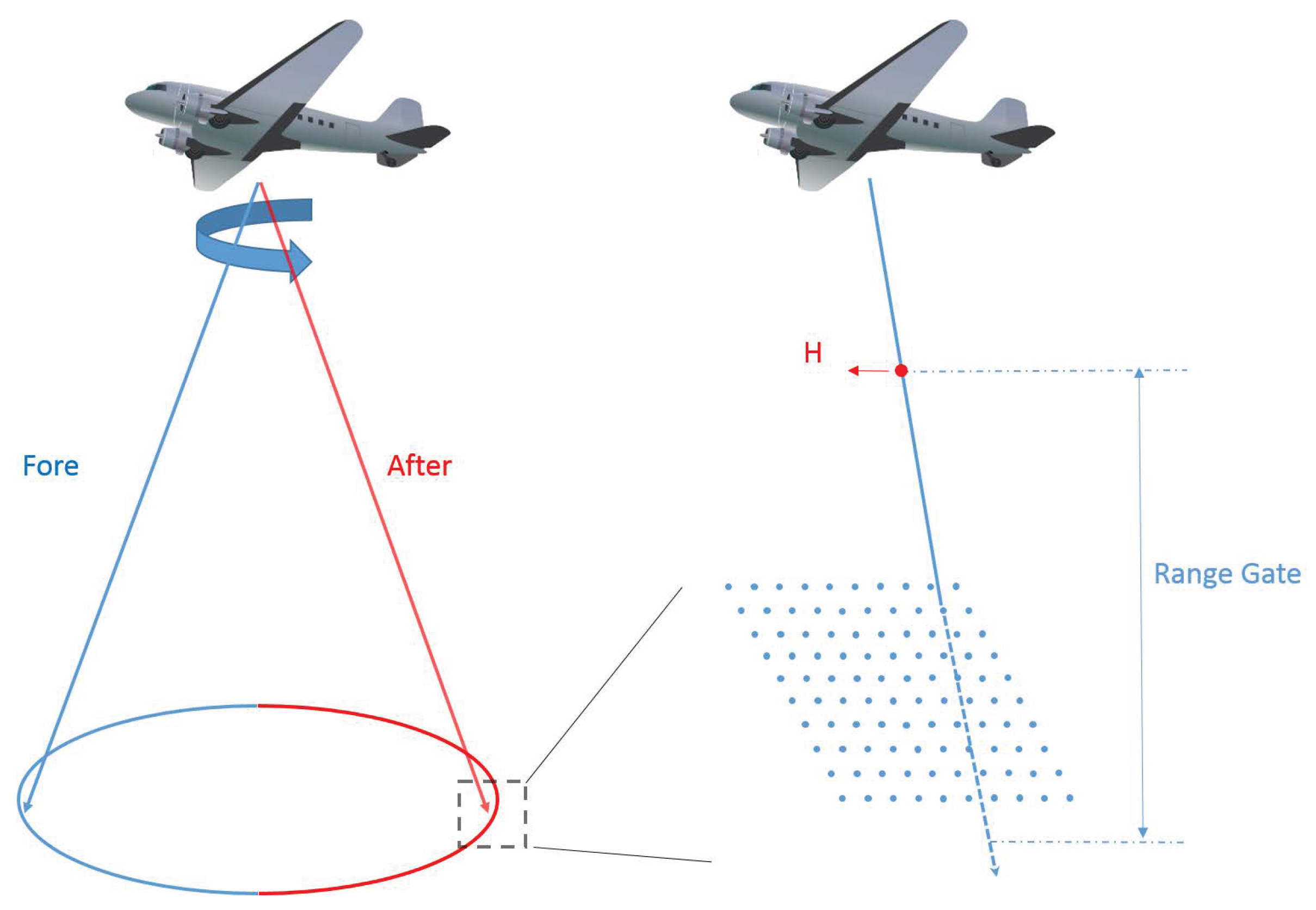
The experimental datasets were collected using the SPL-100 system developed by Sigma Space Corporation (Lanham, MD, USA) and Leica Geosystems Inc. (Lanham, MD, USA). The SPL-100 is a moderate altitude Lidar system employing multiple laser beamlets [13,14], where green laser pulses (532 nm) are split into 100 beamlets that image the target with a 10 × 10 array of illuminated footprints. A circular scanning pattern [15] is used by the SPL-100 and the recorded data are divided into two datasets, fore and after looking, as shown in Figure 1. The first experimental dataset was collected on 10 November 2016 in Easton, MA, USA and contains three overlapping flightlines. Data collection was from ∼3.5 km above ground level (AGL) with a half cone angle of 9 and scan frequency of 25 Hz and pulse repetition frequency (PRF) of 60 KHz. The point density is ∼18 points/m2 for a single flightline and the dataset was truncated with a range gate of 300 m around the expected signal return location. The other experimental dataset was collected on 23 February 2017 in a rural area near Lufkin, TX, USA and also contains three overlapping flightlines. The aircraft flew at ∼2 km AGL with a half cone angle of 15 and PRF of 50 kHz. The point density is ∼20 points/m2 for a single flightline pass and the dataset was truncated with a range gate of 85 m.
2.2. Methodology
The filtering workflow for the combined point cloud is comprised of three steps: (A) tiling the raw data into data blocks; (B) estimating point density using the VS model; and (C) removing noise returns with a modified and improved AES method. Details of each step are given in the following subsections.
2.2.1. Data Tiling
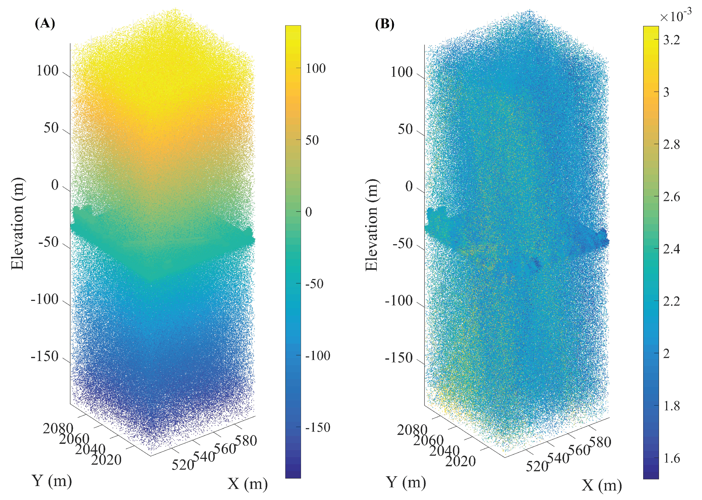
The study datasets were gridded with a horizontal grid size of 100 m × 100 m using TerraScan software. An individual file is generated that contains all the points within the grid cell. In addition to the 3D coordinates in the Universal Transverse Mercator (UTM) coordinate system, the GPS time, channel number and line point density are also encoded in each laser return. Line point density is calculated from the raw single epoch observation dataset by counting the average number of noise points per meter for each laser beamlet. More details about the calculation of line point density are given in [8]. Figure 2 shows a representative data block and line point density for each point.
2.2.2. Voxel Spherical (VS) Model
As previously mentioned, the noise density varies both horizontally and along the laser line-of-sight. Therefore, the noise density for the whole dataset needs to be adaptively estimated instead of computing a single noise metric based on analysis of the noise returns known a priori, which is usually employed to compute a single estimate of noise density [8]. Herein, the points are grouped into voxels and the voxel noise density is estimated and assigned to all the points inside the voxel. It is safe to assume that the noise density is relatively constant for a voxel with a small area, for example 10 × 10 × 10 m, which is the voxel volume used in this paper. A sphere located at the center of the voxel is then defined with the same volume as the voxel. Next, the expected number of noise points in the sphere is estimated. For every point in the data block, the corresponding aircraft location can be interpolated using the post-processed GNSS/INS (Global Navigation Satellite System/Inertial Navigation System) aircraft trajectory. The line-of-sight vector connecting the data point and the aircraft location at laser emission describes the direction of the outgoing laser beamlet. By calculating the distance between the line vector and the center of the sphere, it can be determined if the laser beamlet intersects the sphere. Given the spatial relationship among the query data point Q, the corresponding aircraft location F and the sphere center O, as shown in Figure 3, the distance between the laser beamlet and the sphere center is calculated by the following equation.
The laser beamlets with distance to the center shorter than the radius intersect the sphere. The part of a laser beamlet inside the sphere is labeled red in Figure 3 and its length l can be easily calculated using the Pythagorean Theorem. By applying this process to each data point in the block, all the laser beamlets intersecting the sphere can be obtained along with the corresponding length of the line segment inside the sphere. Then, the estimated density of noise points inside the sphere can be calculated as
where is the line point density of the ith laser beamlet which is calculated according to the methodology detailed in [8]. is the length of part of the ith beamlet inside the sphere, r is the sphere radius and is a correction coefficient which is the ratio of the number of laser shots to the number of beamlets n in the sphere. The correction coefficient compensates for the channels with no returns recorded. Figure 3 shows the entire process flow of the VS model.
2.2.3. Adaptive Ellipsoid Search (AES)
From the previous subsection, the expected number of noise points inside the voxel was estimated. Next, the actual number of neighboring points are calculated and will be used as the basis for determining noise returns. Instead of counting the number of neighbor points directly, it is calculated based on local geometry information. When considering local geometry information, the near-signal noise returns can be effectively removed. For each query point, its 15 nearest neighbors are selected and a Principle Component Analysis (PCA) [16] of their 3D coordinates is computed to obtain three principle components and three corresponding eigenvalues. Then, a base sphere with a radius of is defined at the query point center. The base sphere morphs into an ellipsoid with directionality defined by the local point cloud neighborhood based on the three eigenvalues using the following equations
where a, b and c are the three axis of the ellipsoid and , and are the three eigenvalues. The orientation of the ellipsoid is then modified to better fit local point geometry. To make this transformation simple, instead of rotating the ellipsoid, all the points within the data block are transformed using the following equation
where is the coordinate of the ith point and are the corresponding rotated coordinates. P is a 3 × 3 transform matrix comprised of three principle components. It is then easy to check if a point is located inside the ellipsoid using the following equation
If flag is less than 1, the point is inside the ellipsoid. The number of points that reside in the ellipsoid are then counted for the whole data block. With the expected number of noise returns and the actual number of points in the ellipsoid, a hypothesis test can be established: H0:, the query point is a noise return; and H1, the query point is a signal return.
For a given query point and a region of any shape around it, the number of neighbor points inside the region conforms to a Poisson distribution; the proof is as follows. Consider a 3D space with randomly distributed points. For any point, the probability of the number of its neighbor points inside the region is calculated as
where k is the number of neighbors, v is the volume of the region, is the volume of the whole space and N is the total number of points in the space. When and N are very large, the equation can be approximated as
the point density can then be defined as , and the equation rewritten as
The density is obtained from the VS model by dividing the expected number of points by the volume of the voxel. If the cumulative probability from zero to k is less than 95%, then the null hypothesis H0 is true and the point is a noise return, otherwise the point is a signal return.
3. Results and Discussion
3.1. Results
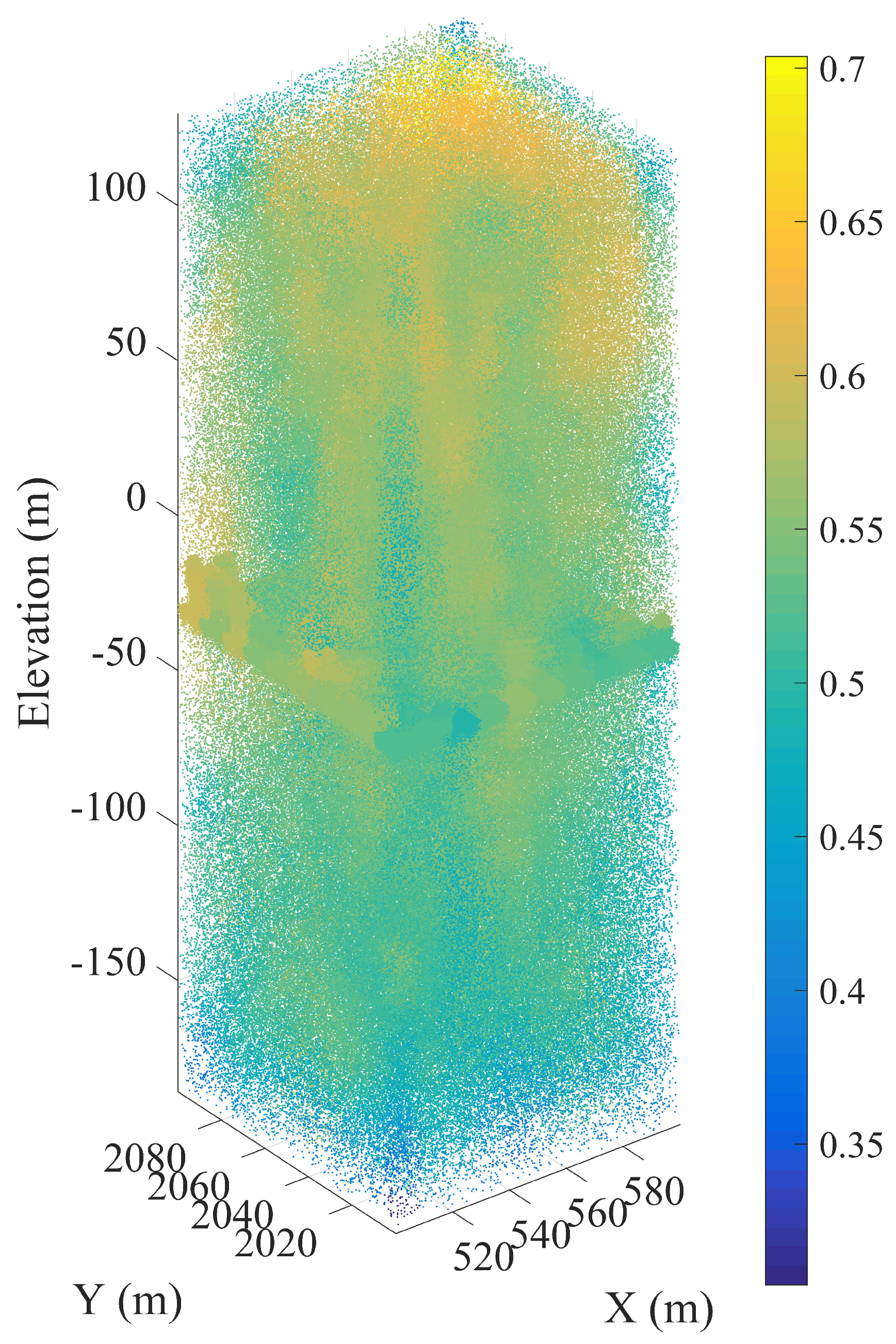
The VS model was first applied to each data block. Figure 4 displays the results for a representative VS model where it can be seen that the noise density is uneven throughout the whole data block. This demonstrates the importance of considering the scanning geometry when estimating noise level.
The filtered result with both VS and AES applied is shown in Figure 5. For comparison, the filtered result for the same area using a histogram method and the original AES method are also shown. The histogram method proposed by Degnan was used; more details on this method can be found in [1,4].
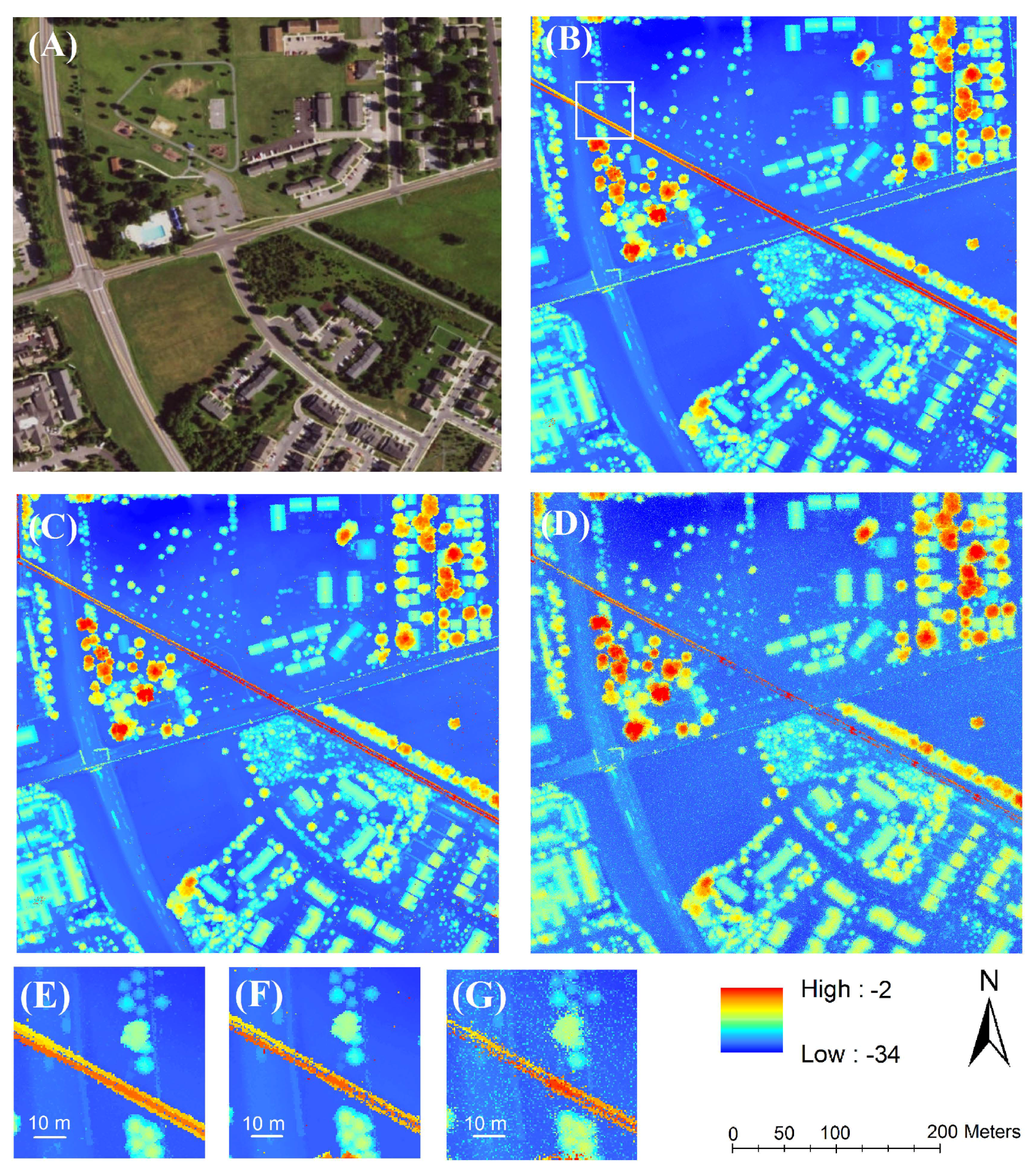
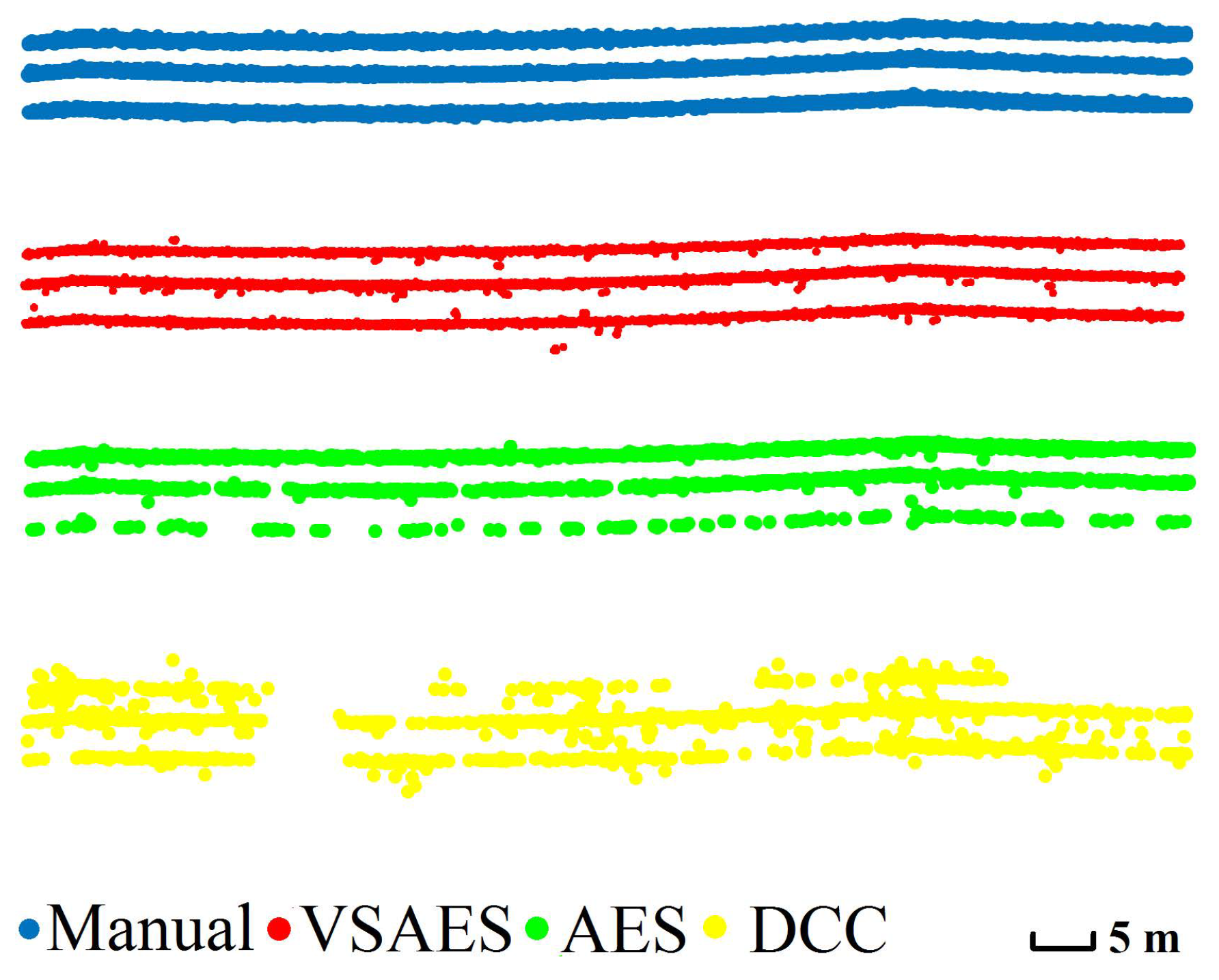
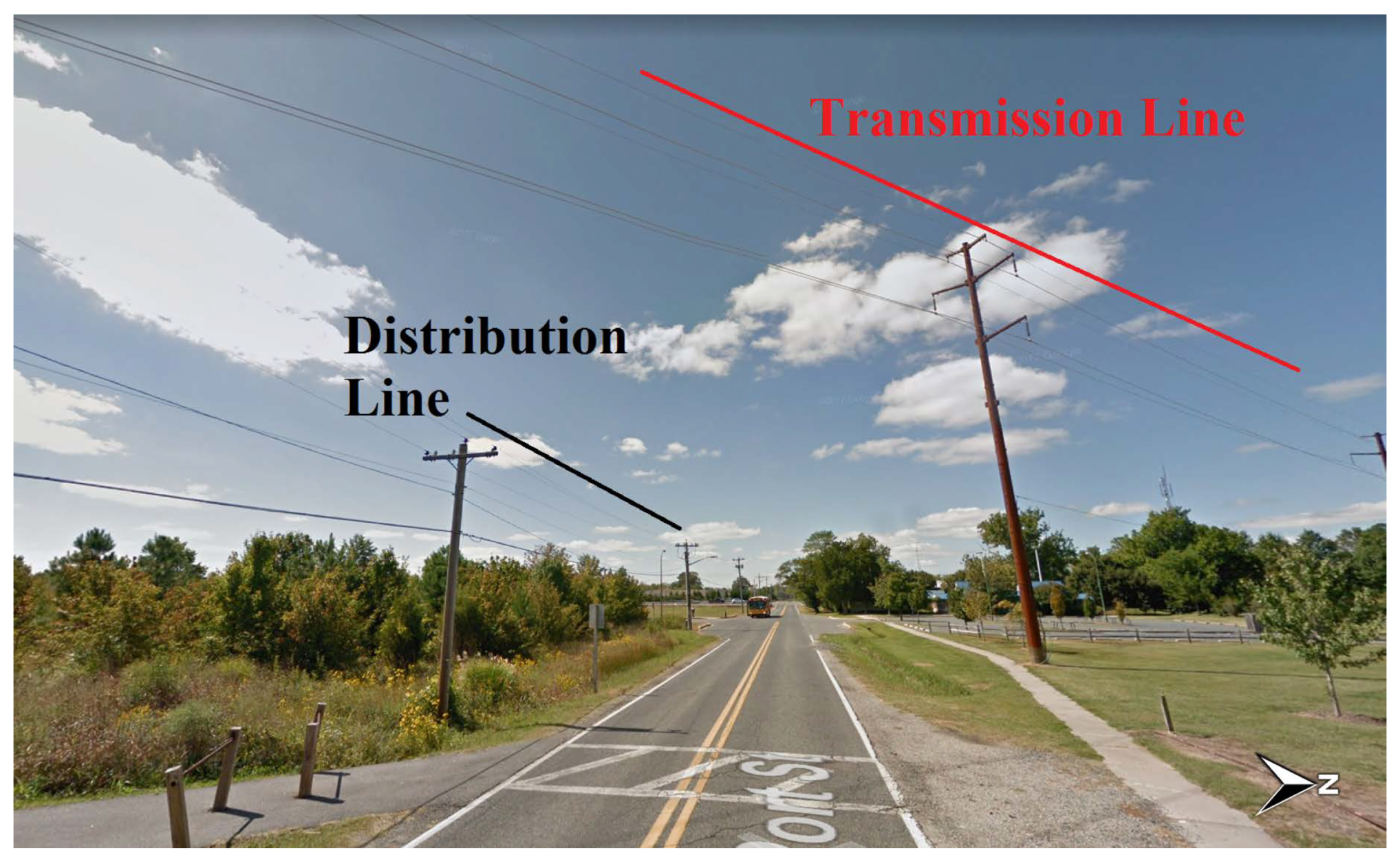
The red linear feature crossing Figure 5 from the top left to bottom right is a transmission line. Significant differences in the appearance of this transmission line can be noted when comparing the three filtered results. The transmission line returns have also been manually classified for comparison with the automatically filtered results. Figure 6 shows vertical profiles of the filtered and manually classified transmission line and Table 1 gives a comparison of the filtered and manually classified datasets. A 7 m × 7 m (height × width) examination region is defined around the transmission line and the number of laser returns automatically classified as signal from the transmission line within it are counted. These points are then compared with the number of manually classified transmission points.
In Table 1, the proposed method retains 89.1% of the power line points with only a few incorrectly classified noise returns. For comparison, AES keeps only 25.9% of the transmission line points and the DCC method retains only 13.4%. In Figure 6, the transmission line points retained in the VSAES results discriminate the three separate cables clearly even though a few noise points remain misclassified close to the wires. For the AES result, the upper two lines are well defined, but the extraction of the third line is not complete with a large number of gaps appearing. For the DCC result, clear gaps can be found in all three cables and more noise points appear close to the transmission lines. An optical image of the transmission lines is displayed in Figure 7. Both a qualitative visual check of the profile views in Figure 6 and the statistical analysis presented in Table 1 show that the extraction of weak signal points is significantly improved by combining the temporally spaced lidar observations and using the adaptive VSAES filtering approach.
Next, the results for a distribution line whose wires have an even smaller diameter than the transmission line are analyzed. As before, the signal points for the distribution line were manually extracted. One thing to note is that because of the low laser energy returned from distribution lines, even manual extraction is very hard and its accuracy is likely lower than that for larger transmission lines. Again, an examination region with the same size, 7 m × 7 m (height × width) was defined to evaluate the performance of the three filters; the statistics for distribution line extraction are given in Table 2 and vertical profiles are shown in Figure 8.
For the extraction of distribution lines, the proposed VSAES method detects only 60% of the line points, but this is still significantly more than the 29.3% for the AES method and 11.1% for the DCC method. In Figure 8, the lowest wire in the VSAES profile is well detected with only a small gap. The top line has more gaps but there are still enough return points to accurately depict the distribution wire geometry. Results for the middle wire are the worst, with larger areas containing gaps. However, the results are still markedly better than for the other two filtering methods, and appear to contain enough points to adequately model all of the distribution lines. An optical image of the distribution lines is also displayed in Figure 7.
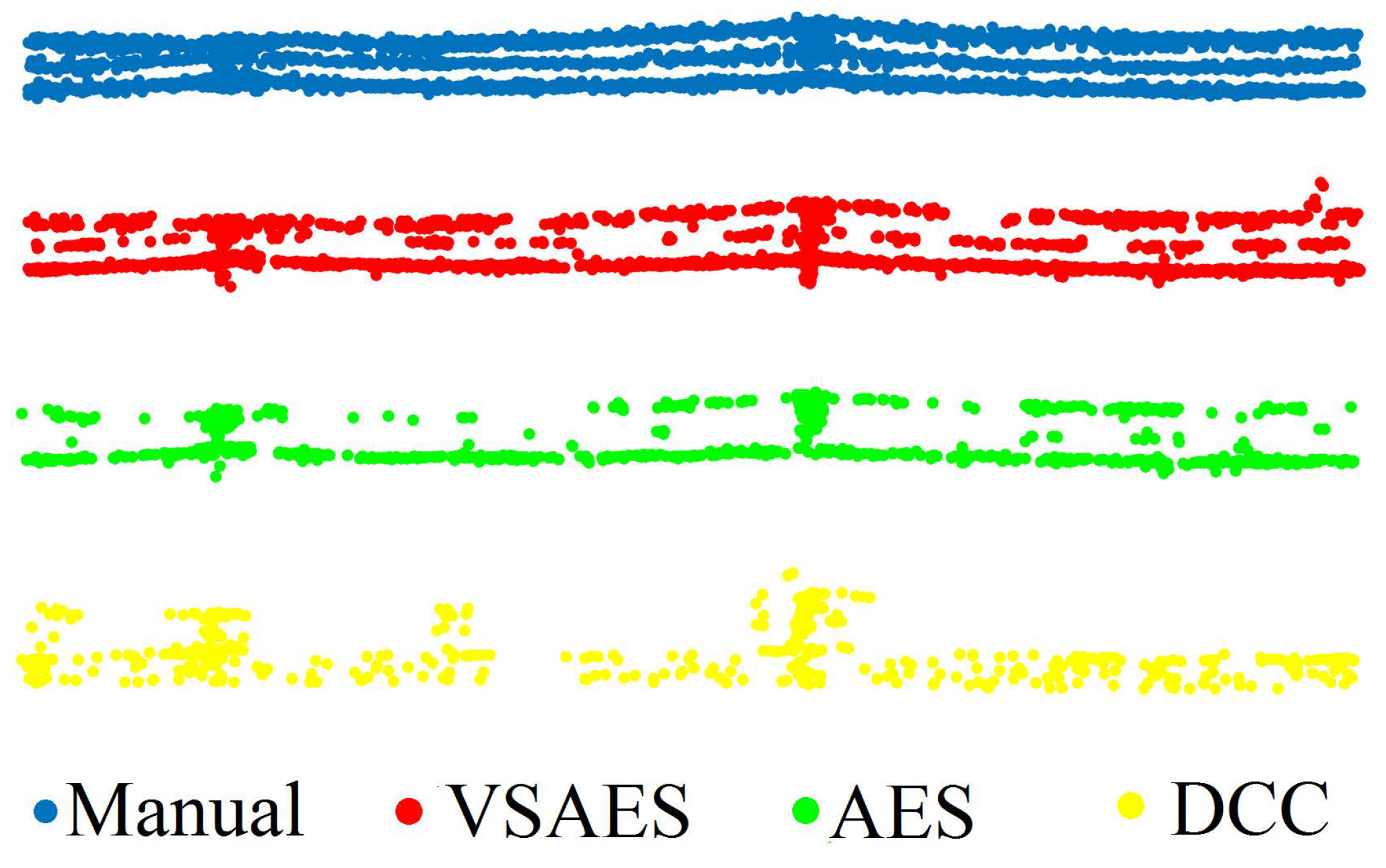
Finally, the performance for an additional power line captured in the Lufkin experimental dataset is examined. The filtered results using VSAES, AES, and DCC are displayed in Figure 9. The detailed sub figures (E, F and G) in Figure 9 show a region at an intersection of two distribution lines. Results from the proposed method retain both lines and clearly shows two lines. Only one line can be seen clearly from the AES results while the other is difficult to see. For the DCC results, no linear features are visible. Vertical profiles and statistical analysis for the three filtered results on the Lufkin dataset are given in Figure 10 and Table 3.
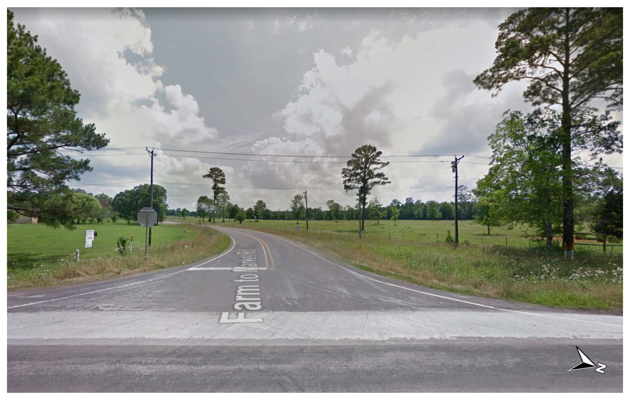
The proposed method significantly outperformed both the AES and DCC methods by correctly classifying 85.9% of distribution line points versus 37.9% and 6.1%, respectively, for the other methods. The top wire in the VSAES result is well extracted, while a few gaps can be found on the middle and bottom wires. By visual inspection of an oblique street view image (Figure 11), it can be seen that there are three top wires and one wire at the middle and bottom levels, respectively. Thus, the top line in the vertical profile is composed of signal returns from three power lines, resulting in a clear line with no gaps in the profile figure.
3.2. Discussion
From the comparison of filtered results from the three sets of powerlines, significant improvement in automatically extracting powerline points can be seen by using the proposed method. The improvements seen in the VSAES results are primarily because of two factors: the adaptive consideration of the local point cloud geometry during filtering and the combination of overlapping flight lines before filtering. Due to the high linearity of the powerlines points, the calculated three dimensional point density for each wire point is relatively small. The DCC method filters SPL data using the resolution of a one dimensional range bin and retains all the points in the data bin as signal points if the query data bin satisfies the filtering criteria. This 1D filtering mechanism makes DCC have limited efficiency for weak signal returns such as those from powerlines. However, if the linearity of the powerline is considered (adapting to the local point cloud geometry), then VSAES can more effectively extract power line points compared to methods that do not consider the local geometrical characteristics of the point cloud.
In addition, due to the small cross-section of the laser footprints on the powerlines, there are only a small number of signal photons bounced back to the SPL detector. Because of the statistical nature of the sensor (i.e., relatively low photon detection efficiency), even fewer photons are recorded by the system, making them difficult to distinguish from noise within a single flightline. In these circumstances, even considering the local geometric information with the AES method is not sufficient to effectively retain enough powerline points; all observations from all overlapping flightlines need to be considered simultaneously, and the proposed VSAES method can fully utilize data from different observations and even different flightline collections by adaptively estimating local noise density. The powerlines are illuminated from different directions and the probability that the sensor receives photons from each part of the powerline is therefore increased, which enhances the spatial correlation of the powerline points and helps to improve the filtered results.
An additional advantage of VSAES over AES is the mathematical robustness of the former method. Even though both VSAES and AES consider local geometric information through a PCA, they utilize different measures to differentiate signal from noise. In AES, several neighbors for a query point within a sphere and then an ellipsoid determined by PCA are counted; the difference between these two numbers of neighbors is used as the decision measure and compared to an empirically determined threshold. The performance of the filtered results relies on a proper selection of this threshold. By contrast, the proposed VSAES method utilizes a filtering criteria based on a hypothesis test and the selection of a statistical 95% confidence threshold instead of an empirically determined threshold, therefore the VSAES is a more robust method.
One last thing to note is that even considering the enhanced spatial correlation and local geometry distribution from overlapping flight observations, there are still a number of powerline points missing; for example, the results for the distribution line in the Easton study area (shown in Figure 8). By checking the corresponding optical image (shown in Figure 11), it is observed that the top and middle lines are of smaller diameter than the bottom one and this likely explains the higher number of missing points for them. For a direct comparison a laser scanning dataset for the same distribution line collected with a linear-mode airborne Lidar system was also examined. The data were collected on 14 June 2016 using a Leica ALS 80 sensor operated at ∼1.3 km AGL and a nominal point density of ∼25 points/m2. The top view and vertical profile of the distribution line from the linear-mode data are shown in Figure 12. From the vertical profile, it can be seen that, even though the bottom wire is well defined, the top and middle lines are missing in the linear-mode data. The energy of the return signal is too low for the linear-mode system to detect, and would require an even lower flight height to capture these lines. However, in the SPL point cloud (flown at ∼2 km AGL), the top and middle lines are defined with enough points to model them. This also indicates that SPL has an advantage over LML for powerline mapping because the data can be collected from a higher flight altitude, which would greatly improve collection efficiency.
4. Conclusions
In this study, an improved VSAES algorithm was proposed to extract weak signal points from SPL point clouds, and the methodology was tested using examples from powerlines. The proposed method first reorganizes the combined data by tiling them into data blocks, during which the spatial correlation of the signal points is improved. The VS model is then used to estimate the expected number of noise points in each voxel and adaptively compensates for uneven noise density while also balancing computational load. Finally, an improved AES method, based on a hypothesis test, is used to filter the data. The combined VSAES method is used on a complete SPL dataset (instead of on a flightline by flightline basis) and makes a significant improvement for the extraction of weak signal returns from powerlines. In the first experimental area in Easton, MD, 89% of the transmission line points were correctly extracted versus 25.9% for the AES method and 13.4% for the DCC method. For a distribution line, whose return signals are even weaker (due to smaller wire diameter), the proposed VSAES method extracted 60% of the signal points versus 29.3% for AES and 11.1% for DCC. For the second Lufkin dataset, the VSAES extraction results had 85.9% correctly classified versus 37.9% and 6.1% for AES and DCC respectively. It was also demonstrated with coincident LML data that points from thin powerlines, which are not recorded in the LML data, can be detected from SPL data, even though the SPL system was flown at a higher AGL and with a wider swath coverage. The high quantum sensitivity and high data collection efficiency of the SPL system shows great potential for wide area powerline mapping and monitoring.
Author Contributions
X.W. designed the experiments, compiled the results and wrote the initial version of the manuscript. C.G. assisted in experiment design and analysis of the results and edited and modified the manuscript to the current version. Z.P. provided access to raw data samples and formats, assisted in methodology and experiment design and reviewed the final manuscript for technical content.
Funding
This research was funded in part by the National Aeronautics and Space Administration under grant NNX15AQ22G, the U.S. Army Engineer Research and Development Center Cold Regions Research and Engineering Laboratory Remote Sensing/GIS Center of Expertise and Leica Geosystems.
Acknowledgments
The authors would like to thank Preston Hartzell for reviewing an earlier version of this manuscript. The authors would also like to thank the four anonymous reviewers, whose constructive comments and criticisms greatly improved the final version of the manuscript.
Conflicts of Interest
The authors declare no conflict of interest.
References
- Degnan, J.J.; Field, C.T. Moderate to high altitude, single photon sensitive, 3D imaging lidars. In Advanced Photon Counting Techniques; International Society for Optics and Photonics: Bellingham, WA, USA, 2014; Volume 9114. [Google Scholar]
- Tang, H.; Swatantran, A.; Barrett, T.; DeCola, P.; Dubayah, R. Voxel-Based Spatial Filtering Method for Canopy Height Retrieval from Airborne Single-Photon Lidar. Remote Sens. 2016, 8, 771. [Google Scholar] [CrossRef]
- Swatantran, A.; Tang, H.; Barrett, T.; DeCola, P.; Dubayah, R. Rapid, High-Resolution Forest Structure and Terrain Mapping over Large Areas using Single Photon Lidar. Sci. Rep. 2016, 6, 28277. [Google Scholar] [CrossRef] [PubMed] [Green Version]
- Degnan, J.J. Photon-counting multikilohertz microlaser altimeters for airborne and spaceborne topographic measurements. J. Geodyn. 2002, 34, 503–549. [Google Scholar] [CrossRef] [Green Version]
- Gwenzi, D.; Lefsky, M.A. Prospects of photon counting lidar for savanna ecosystem structural studies. ISPRS Int. Arch. Photogramm. Remote Sens. Spat. Inf. Sci. 2014, 40, 141–147. [Google Scholar] [CrossRef]
- Herzfeld, U.C.; McDonald, B.W.; Wallin, B.F.; Neumann, T.A.; Markus, T.; Brenner, A.; Field, C. Algorithm for Detection of Ground and Canopy Cover in Micropulse Photon-Counting Lidar Altimeter Data in Preparation for the ICESat-2 Mission. IEEE Trans. Geosci. Remote Sens. 2014, 52, 2109–2125. [Google Scholar] [CrossRef] [Green Version]
- Moussavi, M.S.; Abdalati, W.; Scambos, T.; Neuenschwander, A. Applicability of an automatic surface detection approach to micro-pulse photon-counting lidar altimetry data: Implications for canopy height retrieval from future ICESat-2 data. Int. J. Remote Sens. 2014, 35, 5263–5279. [Google Scholar] [CrossRef]
- Wang, X.; Glennie, C.L.; Pan, Z. An Adaptive Ellipsoid Searching Filter for Airborne Single-Photon Lidar. IEEE Geosci. Remote Sens. Lett. 2017, 14, 1258–1262. [Google Scholar] [CrossRef]
- Cheng, L.; Tong, L.; Wang, Y.; Li, M. Extraction of Urban Power Lines from Vehicle-Borne LiDAR Data. Remote Sens. 2014, 6, 3302–3320. [Google Scholar] [CrossRef] [Green Version]
- McLaughlin, R.A. Extracting Transmission Lines From Airborne LiDAR Data. IEEE Geosci. Remote Sens. Lett. 2006, 3, 222–226. [Google Scholar] [CrossRef]
- Matikainen, L.; Lehtomäki, M.; Ahokas, E.; Hyyppä, J.; Karjalainen, M.; Jaakkola, A.; Kukko, A.; Heinonen, T. Remote sensing methods for power line corridor surveys. ISPRS J. Photogramm. Remote Sens. 2016, 19, 10–31. [Google Scholar] [CrossRef]
- Zhu, L.; Hyyppä, J. Fully-Automated Power Line Extraction from Airborne Laser Scanning Point Clouds in Forest Areas. Remote Sens. 2014, 6, 11267–11282. [Google Scholar] [CrossRef]
- Degnan, J.J. Multibeam, Single Photon Lidars for Rapid, Large Scale, High Resolution, Topographic and Bathymetric Mapping. Remote Sens. 2016, 8, 958. [Google Scholar] [CrossRef]
- Degnan, J.J.; Wells, D.; Machan, R.; Leventhal, E. Second generation airborne 3D imaging lidars based on photon counting. In Advanced Photon Counting Techniques; International Society for Optics and Photonics: Bellingham, WA, USA, 2007; Volume 6771. [Google Scholar]
- Pan, Z.; Hartzell, P.; Glennie, C.L. Calibration of an Airborne Single-Photon Lidar System With a Wedge Scanner. IEEE Geosci. Remote Sens. Lett. 2017, 14, 1418–1422. [Google Scholar] [CrossRef]
- Wold, S.; Esbensen, K.; Geladi, P. Principle Component Analysis. Chemom. Intell. Lab. Syst. 1987, 2, 37–52. [Google Scholar] [CrossRef]
Figure 1.
An overview of the SPL100 scanning pattern: (left) fore and after observation data; and (right) the details of one laser shot and beamlet vectors. The transmitted laser pulse is split into 100 beamlets and the footprints form a 10 × 10 array on the target. A range gate is used to truncate the raw data. H is the highest point in one beamlet vector, i.e., the start of the range gate.

Figure 2.
An overview of a 100 m × 100 m data block after tiling: (A) colored by elevation; and (B) colored by estimated line point density.
Figure 2.
An overview of a 100 m × 100 m data block after tiling: (A) colored by elevation; and (B) colored by estimated line point density.

Figure 3.
Workflow for the VS model. The data block is first voxelized into 10 × 10 × 10 m voxels. Then, for each point, a sphere with the same volume as the voxel is defined at the center of the voxel. Finally, the expected number of noise points is calculated based on the geometry of the data points and the corresponding aircraft trajectory.
Figure 4.
Estimated expected number of noise points for a representative voxel using the VS model. The data are colored by the expected number of noise returns.
Figure 4.
Estimated expected number of noise points for a representative voxel using the VS model. The data are colored by the expected number of noise returns.

Figure 5.
Satellite image and filtered SPL point clouds for the Easton study area: satellite image (A); VSAES result (B); AES only result (C); and DCC result (D). Detailed view of a portion of a powerline (E–G) corresponding to (B–D). The extents are labeled in (B) with a white square. The filtered results are colored by elevation.

Figure 6.
Vertical profile of the transmission line from manually selected raw data and filtered results using the VSAES, AES and DCC methods.
Figure 6.
Vertical profile of the transmission line from manually selected raw data and filtered results using the VSAES, AES and DCC methods.

Figure 7.
Ground view image of the Easton study area. The red line depicts the transmission lines and the black line shows the distribution lines. The north arrow shows an approximate north direction.
Figure 7.
Ground view image of the Easton study area. The red line depicts the transmission lines and the black line shows the distribution lines. The north arrow shows an approximate north direction.

Figure 8.
Vertical profile of the distribution lines from manually selected raw data and filtered result using the VSAES , AES and DCC methods.
Figure 8.
Vertical profile of the distribution lines from manually selected raw data and filtered result using the VSAES , AES and DCC methods.

Figure 9.
Satellite image and filtered single photon lidar results for the Lufkin area: satellite image of study area (A); VSAES result (B); AES only result (C); and DCC result (D). Detailed view of a portion of the powerline (E–G) corresponding to (B–D). The extents are labeled in (B) with a white square. The filtered results are colored by elevation.
Figure 10.
Vertical profile of the transmission lines for Lufkin study area from manually classified raw data and filtered results using VSAES, AES and DCC methods.
Figure 10.
Vertical profile of the transmission lines for Lufkin study area from manually classified raw data and filtered results using VSAES, AES and DCC methods.
Figure 11.
Ground view image of the Lufkin study area. The north arrow shows an approximate north direction.
Figure 11.
Ground view image of the Lufkin study area. The north arrow shows an approximate north direction.

Figure 12.
Plan and profile view of the Lufkin study area distribution line captured using a Leica ALS-80 linear mode lidar system.
Figure 12.
Plan and profile view of the Lufkin study area distribution line captured using a Leica ALS-80 linear mode lidar system.

Table 1.
Statistical results for the automated extraction of transmission lines with the three filtering methods. The detection rate is calculated by dividing the number of correctly identified points with the number of manually classified signal points in the examination region. The false alarm rate is calculated by dividing the number of misclassified points with the total number of extracted points in the examination region.
| # Correctly Identified | Detection Rate | # Misclassified | False Alarm Rate | |
|---|---|---|---|---|
| Raw data | 57,185 | N/A | N/A | N/A |
| VSAES | 50,925 | 89.1% | 2884 | 5.4% |
| AES | 14,802 | 25.9% | 799 | 5.1% |
| DCC | 7666 | 13.4% | 2016 | 20.8% |
Table 2.
Statistical results for the automated extraction of distribution lines with the three filtering methods. The detection rate is calculated by dividing the number of correctly identified points with the number of manually classified signal points in the examination region. The false alarm rate is calculated by dividing the number of misclassified points with the total number of extracted points in the examination region.
| # Correctly Identified | Detection Rate | # Misclassified | False Alarm Rate | |
|---|---|---|---|---|
| Raw data | 20,793 | N/A | N/A | N/A |
| VSAES | 12,265 | 60.0% | 1042 | 7.8% |
| AES | 6089 | 29.3% | 594 | 8.9% |
| DCC | 2305 | 11.1% | 639 | 41.6% |
Table 3.
Statistical results for the automated extraction of distribution lines using three filtering methods. The detection rate is calculated by dividing the number of correctly identified points with the number of manually classified signal points in the examination region. The false alarm rate is calculated by dividing the number of mis-classified points with the total number of extracted points in the examination region.
| # Correctly Identified | Detection Rate | # Misclassified | False Alarm Rate | |
|---|---|---|---|---|
| Raw data | 104,542 | N/A | N/A | N/A |
| VSAES | 89,836 | 85.9% | 5250 | 5.5% |
| AES | 39,367 | 37.9% | 2622 | 6.2% |
| DCC | 6370 | 6.1% | 980 | 13.3% |
© 2018 by the authors. Licensee MDPI, Basel, Switzerland. This article is an open access article distributed under the terms and conditions of the Creative Commons Attribution (CC BY) license (http://creativecommons.org/licenses/by/4.0/).
Share and Cite
MDPI and ACS Style
Wang, X.; Glennie, C.; Pan, Z. Weak Echo Detection from Single Photon Lidar Data Using a Rigorous Adaptive Ellipsoid Searching Algorithm. Remote Sens. 2018, 10, 1035. https://doi.org/10.3390/rs10071035
AMA Style
Wang X, Glennie C, Pan Z. Weak Echo Detection from Single Photon Lidar Data Using a Rigorous Adaptive Ellipsoid Searching Algorithm. Remote Sensing. 2018; 10(7):1035. https://doi.org/10.3390/rs10071035
Chicago/Turabian StyleWang, Xiao, Craig Glennie, and Zhigang Pan. 2018. "Weak Echo Detection from Single Photon Lidar Data Using a Rigorous Adaptive Ellipsoid Searching Algorithm" Remote Sensing 10, no. 7: 1035. https://doi.org/10.3390/rs10071035
Note that from the first issue of 2016, this journal uses article numbers instead of page numbers. See further details here.