Concentric Circle Pooling in Deep Convolutional Networks for Remote Sensing Scene Classification


1
Faculty of Information Engineering, China University of Geosciences (Wuhan), Wuhan 430074, China
2
College of Urban and Environmental Sciences, Central China Normal University, Wuhan 430079, China
3
Soil and Water Conservation Department, Changjiang River Scientific Research Institute, Wuhan 430010, China
4
State Key Laboratory for Information Engineering in Surveying, Mapping and Remote Sensing (LIESMARS), Wuhan University, Wuhan 430079, China
*
Author to whom correspondence should be addressed.
Remote Sens. 2018, 10(6), 934; https://doi.org/10.3390/rs10060934
Submission received: 27 April 2018
/
Revised: 29 May 2018
/
Accepted: 9 June 2018
/
Published: 13 June 2018
(This article belongs to the Section Remote Sensing Image Processing)
Abstract
:Convolutional neural networks (CNNs) have been increasingly used in remote sensing scene classification/recognition. The conventional CNNs are sensitive to the rotation of the image scene, which will inevitably result in the misclassification of remote sensing scene images that belong to the same category. In this work, we equip the networks with a new pooling strategy, “concentric circle pooling”, to alleviate the above problem. The new network structure, called CCP-net can generate a concentric circle-based spatial-rotation-invariant representation of an image, hence improving the classification accuracy. The square kernel is adopted to approximate the circle kernels in concentric circle pooling, which is much more efficient and suitable for CNNs to propagate gradients. We implement the training of the proposed network structure with standard back-propagation, thus CCP-net is an end-to-end trainable CNNs. With these advantages, CCP-net should in general improve CNN-based remote sensing scene classification methods. Experiments using two publicly available remote sensing scene datasets demonstrate that using CCP-net can achieve competitive classification results compared with the state-of-art methods.

1. Introduction
With the development of remote sensing technology, large amounts of Earth-observation images with high resolution are becoming increasingly available and playing an ever-more important role in remote sensing scene classification [1]. High-Resolution Satellite (HRS) images provide much of the appearance and spatial arrangement information that is useful for remote sensing scene category recognition [2]. However, it is difficult to recognize remote sensing scene categories because they usually cover multiple land use categories or ground objects [3,4,5,6,7,8,9,10] such as airports with airplanes, runways, and grass. The classification of HRS images turns from a single remote sensing scene category-based or single object-based classification to a remote sensing scene-based semantic classification [11]. Remote sensing scene categories are largely affected and determined by human and social activities, and the recognition of remote sensing scene image is therefore based on a priori knowledge. As a result of such difficulties, traditional pixel-based [12] and low-level feature-based image classification techniques [13,14] can no longer achieve satisfactory results for remote sensing scene classification.
In the past few years, a large number of feature representation models have been proposed for scene classification. One of the most popularly used models is the Bag-Of-Visual-Words (BOVW) model [15,16,17,18], which provides an efficient solution for remote sensing scene classification. The BOVW model, initially proposed for text categorization, treats an image as a collection of unordered appearance descriptors, and represents the images with the frequency of “visual words” that are constructed by quantizing local features, such as the Scale-Invariant Feature Transform (SIFT) [19] or Histograms of Oriented Gradients (HOGs) [20] with a clustering method (for example, k-means) [15]. The original BOVW method discards the spatial order of the local features and severely limits the descriptive capability of image representation. Therefore, many variant methods [4,21,22,23] based on the BOVW model have been developed for improving the ability to depict the spatial relationships of local features. These methods are based on hand-crafted features, which rely heavily on the experience and domain knowledge of experts. Due to the lack of consideration for the details of actual data, it is difficult with these low-level features to attain a balance between discriminability and robustness [24]. Such features often fail to accurately characterize the complex remote sensing scenes found in HRS images [25].
Deep Learning (DL) algorithms, especially Convolutional Neural Networks (CNNs), have achieved great success in image classification [26], detection [27], and segmentation [28] on several benchmarks [29]. CNN is a hierarchical network invariant to image translations, which is composed of convolutional layers, pooling layers, and fully-connected layers. The key to success is the ability to learn the increasingly complex transformations of the input and to capture invariances from large labelled datasets [30]. However, it is difficult to directly apply the CNNs to remote sensing scene classification for millions of parameters to train the CNNs, which the training samples are insufficient for training. The studies in References [31,32,33,34,35,36,37] have demonstrated that CNNs can be pre-trained on large natural image datasets such as ImageNet [38], which contains general-purposed feature extractors, and can be transferable to many other domains. This is very helpful in the remote sensing scene classification because of the difficulty of training a deep CNN with a small number of training samples. Many approaches utilize the outputs of a deep and fully-connected layer as features to achieve transfer in CNNs. These methods, however, concatenate the outputs of the last convolutional layer to link with the fully-connected layer. This transformation does not capture the information concerning the spatial layout, which has limited descriptive ability in remote sensing scene classification. The works in References [4,25,39] can capture the spatial arrangement for the local features. They are designed for the hand-craft features and are not end-to-end trainable as CNNs are. The Spatial Pyramid Pooling (SPP) [40,41,42,43,44] (popularly known as the Spatial Pyramid Matching or SPM [21]) can incorporate spatial information by partitioning the image into increasingly fine subregions and computing the histograms of local features found inside each subregion. He et al. [41] introduce an SPP layer, which should, in general, improve the CNN-based image classification methods. Nevertheless, this pooling method was designed for natural image scene classification using ordered regular grids that incorporate spatial information into the representation, and therefore, are sensitive to the rotation of image scenes. This sensitivity problem inevitably causes the misclassification of scene images, especially for remote sensing scene images, and influences classification performance. These works in References [45,46] can learn a rotation-invariant CNN model object detection in remote sensing images by using data augmentation method which generates a set of new training samples by rotating transformation. These methods were designed for object detection and the data augmentation operation will inevitably increase the computational cost especially on large dataset because several transformations are required for each training samples.
In this paper, we introduce a Concentric Circle Pooling (CCP) layer to incorporate rotation-invariant spatial layout information of remote sensing scene images. The concentric circle-based partition strategy of an image has been proven effective for rotation-invariant spatial information representation in color and texture feature extraction [47,48] and the BOVW [11] and FV representations [49]. It partitions the image into a series of annular subregions and aggregates the local features found inside each annular subregion. However, concentric circle pooling has not been considered in the context of CNNs for remote sensing images. We applied this strategy to CNN models and designed a new network structure (called CCP-net) for remote sensing scene classification. Specifically, we added a CCP layer on top of the last convolutional layer. The CCP layer pools the convolutional features and then feeds them into the fully-connected layers. Thus, for the CCP layer, using annular spatial bins, we can pool the convolutional features to achieve a rotation invariant spatial representation. The experiments were conducted based on two public ground truth image datasets, manually extracted from publicly available high-resolution overhead imagery. The experimental results show that the CCP layer helps CNNs to represent the remote sensing scene images and achieve high classification accuracies.
The remainder of this paper is organized as follows: Section 2 introduces the proposed CCP layer for remote sensing scene classification. The experimental results and analysis are presented in Section 3, followed by an analysis and discussion in Section 4. In Section 5, some concluding remarks are presented and perspectives on future work close the paper.
2. The Proposed Method
2.1. Deep Convolutional Neural Network
The typical architecture of a CNN is composed of multiple cascaded layers, including convolutional layers, nonlinear pooling layers, and fully-connected layers. The convolutional layer is the core building block of a CNN, which is used to detect local conjunctions of features from the previous layer and mapping their appearance to a feature map. Each element of these feature maps is obtained by computing a dot product between the local region connecting to the input feature maps and a set of weights (called filters or kernels). The pooling layer is responsible for reducing the special size of the activation maps by a downsampling operation along the spatial dimensions of feature maps via computing the aggregated values on a local region. Two different aggregated methods including max pooling and average pooling are conducted through the experiments. The fully-connected layers on the top of several stacked convolutional and pooling layers usually use nonlinear activation functions [50] based on a hyperbolic tangent or rectified linear units (ReLU) [51]. The last fully-connected layer (also called the softmax layer) computes the scores for each defined class using the softmax activate function. The parameters of CNNs are trained with Stochastic Gradient Descent (SGD) based on the backpropagation algorithm [52].
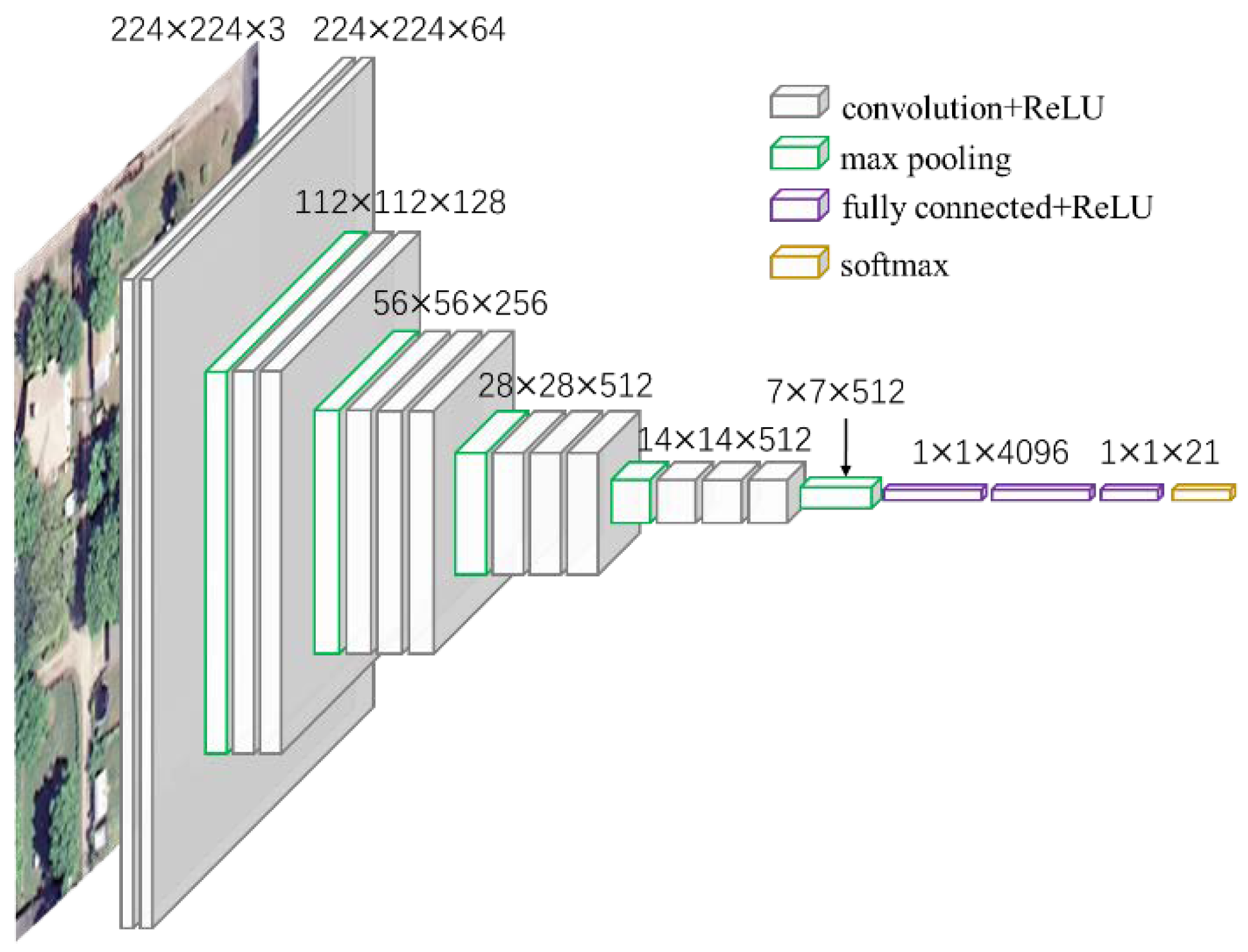
We use a popular architecture, VGG-VD networks [53], which won the runner-up prize in the 2014 ImageNet Large Scale Visual Recognition Challenge (ILSVRC-2014). The VGG-VD models include two very deep CNNs, knowns as VGG-VD16 (containing 13 convolutional layers and 3 fully-connected layers) and VGG-VD19 (containing 16 convolutional layers and 3 fully-connected layers). Figure 1 shows an example architecture using VGG-VD16 for remote sensing scene classification. The input images for VGG-VD16 are required to be resized to 224 × 224 × 3 to be compatible with the fully-connected layers. For the difficulty of training this deep network with small remote sensing datasets, we can employ a pre-trained VGG-VD16 and fine-tune them on scene datasets [54] or simply take the pre-trained CNN as a fixed feature extractor [36].
2.2. Concentric Circle Pooling Layer
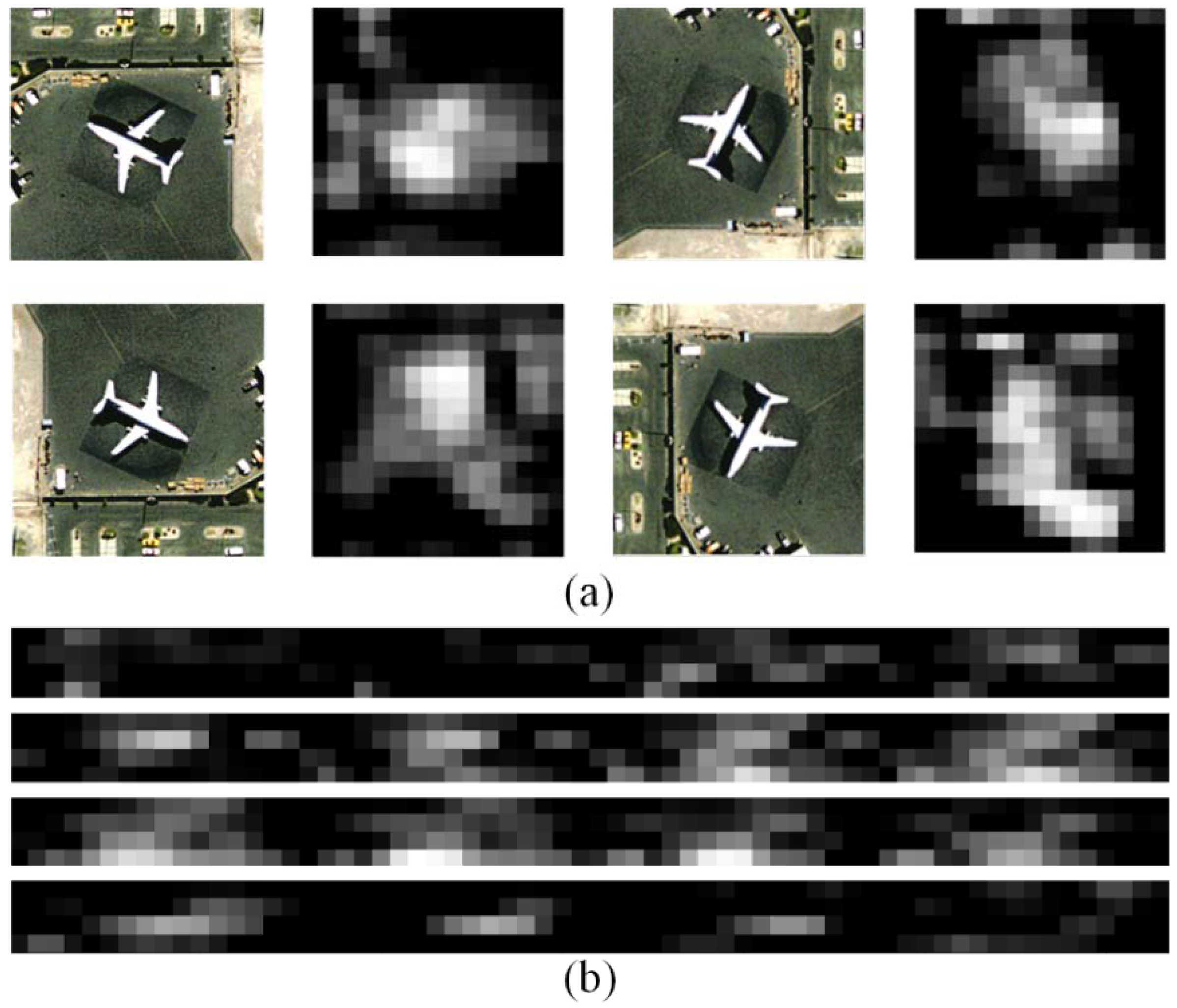
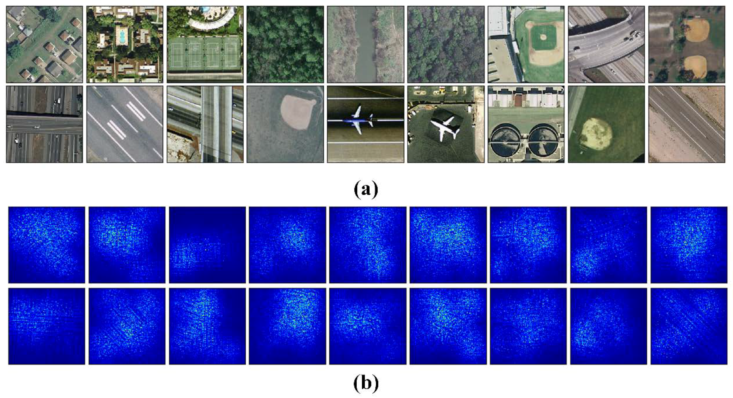
Due to the problem of object rotation variation in the remote sensing scene, it is problematic to directly use CNNs for remote sensing scene classification. Figure 2 illustrates this problem. Take the remote sensing scene image as an example, for Figure 2a, where they all belong to the same scene category. The 16 × 16 grey-scale maps in Figure 2a are one channel of the feature maps extracting by the last convolutional layer of VGG-VD16. The difference among these four feature maps is not simply rotating them. The traditional CNNs flatten the feature maps to connect with fully-connected layers. In Figure 2b, we split each 256-dimensional flattened representation into four parts and = each part in different subgraph. In each subgraph, we can observe that the dissimilarity among these four representations becomes larger. This will limit the capability of CNNs applied to remote sensing applications.
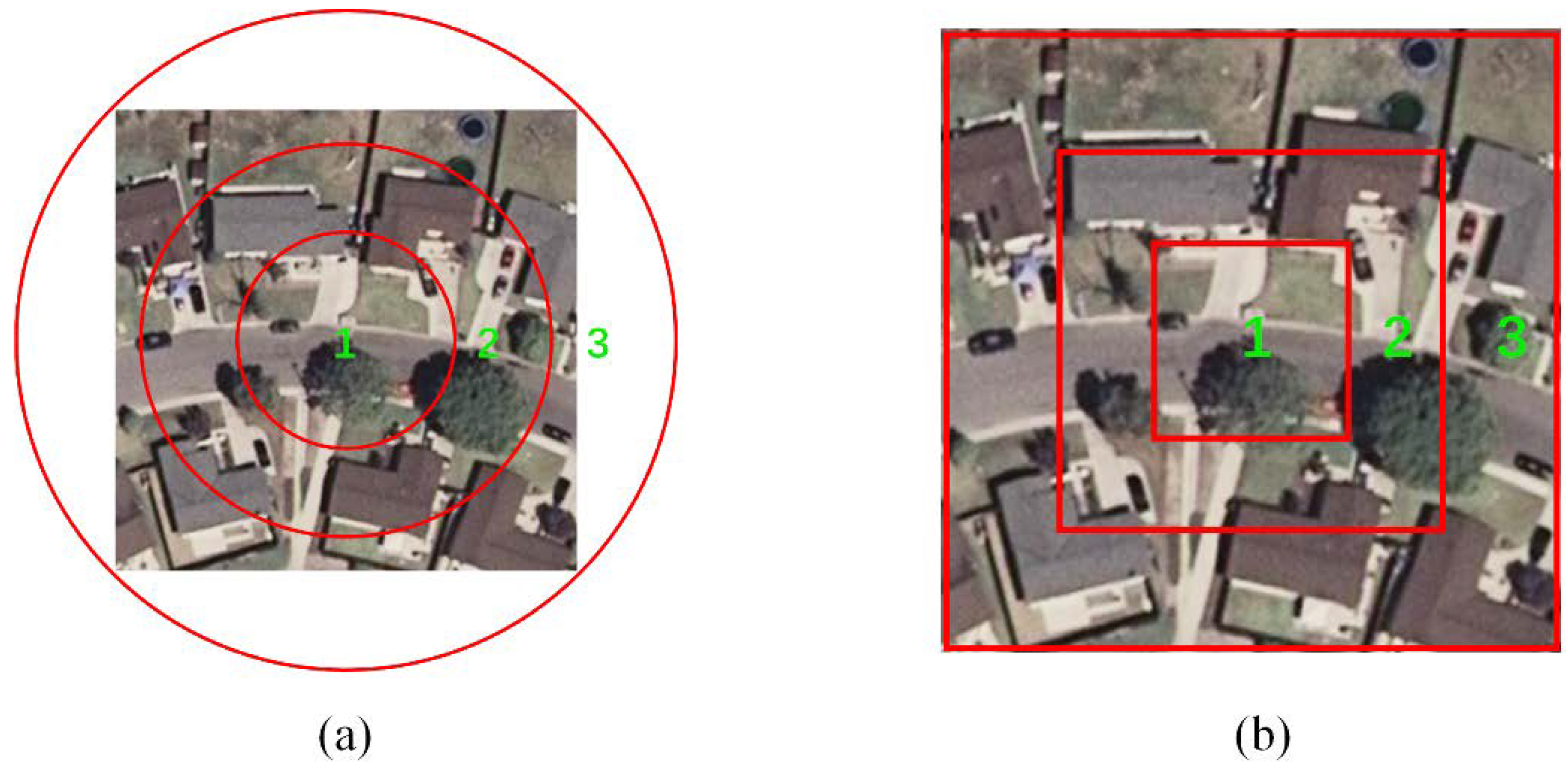
Concentric circle structure, which is used to improve BOVW method for remote sensing scene classification, can maintain spatial and rotation-invariance information by pooling in the local annular subregions (Figure 3a). We can acquire the spatial information of rotation-invariance by using this concentric circle structure to extract the spatial distribution of visual words. Therefore, we introduce the concentric circle pooling to the CNNs to capture the rotation-invariance information for remote sensing scene classification. As shown in Figure 3, circular kernels (Figure 3a) induce rotational invariance, but square kernels (Figure 3b) are computationally more efficient at the partial expense of rotational invariance. Furthermore, square kernels are more suitable for the CNNs to calculate and propagate gradients. Therefore, we adopt the square kernels in our proposed network architecture.
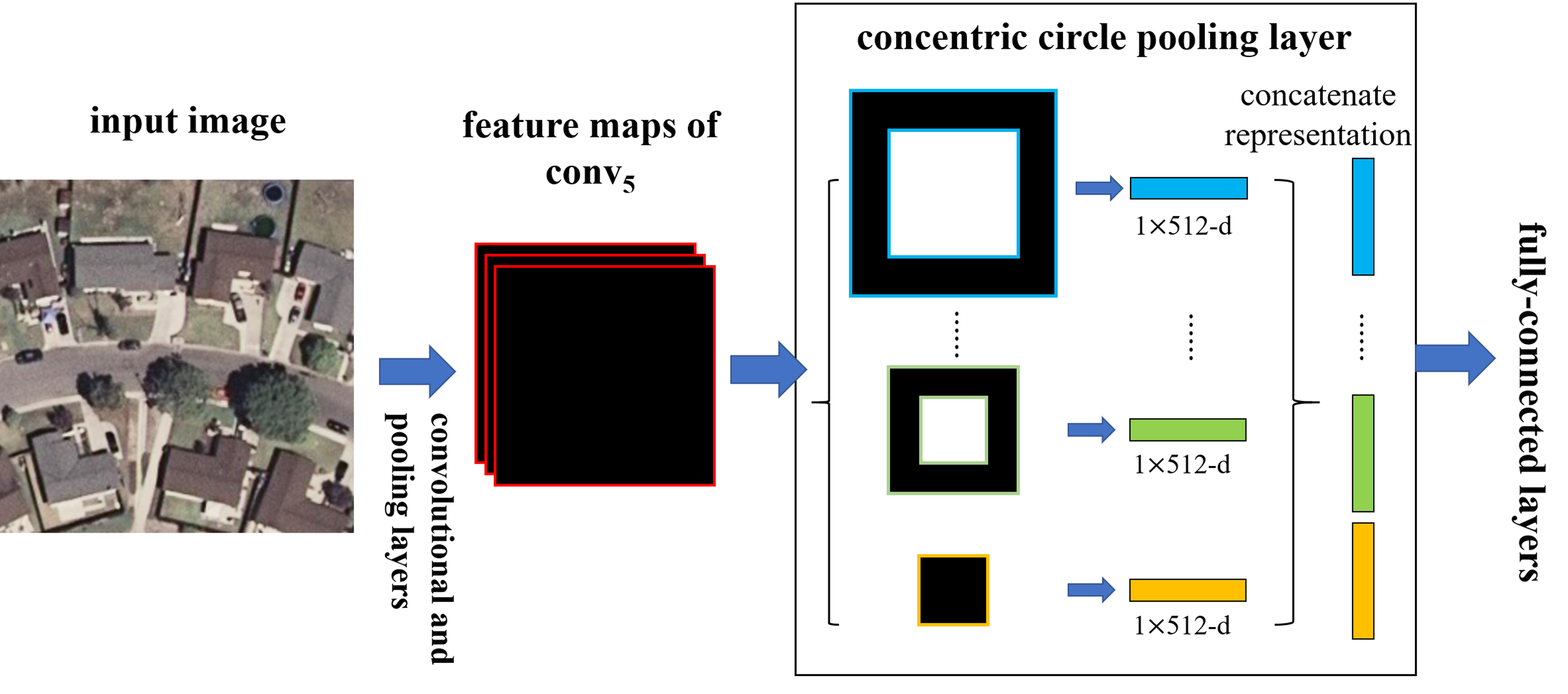
To adopt the deep network for the spatial information of rotation-invariance, we replaced the last pooling layer (the pool5 after the last convolutional layer conv5 in VGG-VD16) with a CCP layer. Figure 4 illustrates our method. In each annular subregion, we pool the response of each filter with max/average pooling. The output size of the last convolutional layer may not divide exactly by the number of subregions, so the valid number of the annular subregion is between 1 and R, where R denotes the circle number, which is the input number of subregions. The outputs of the CCP layer are K-dimensional vectors, where , and K denotes the number of filters in the last convolutional layer. In the next subsection, we interpret the output size of the CCP layer in detail.
2.3. Training the Network
The network with the CCP layer can be trained with standard SGD [52]. We will describe our training procedure using concentric circle pooling and the output size of the CCP layer.
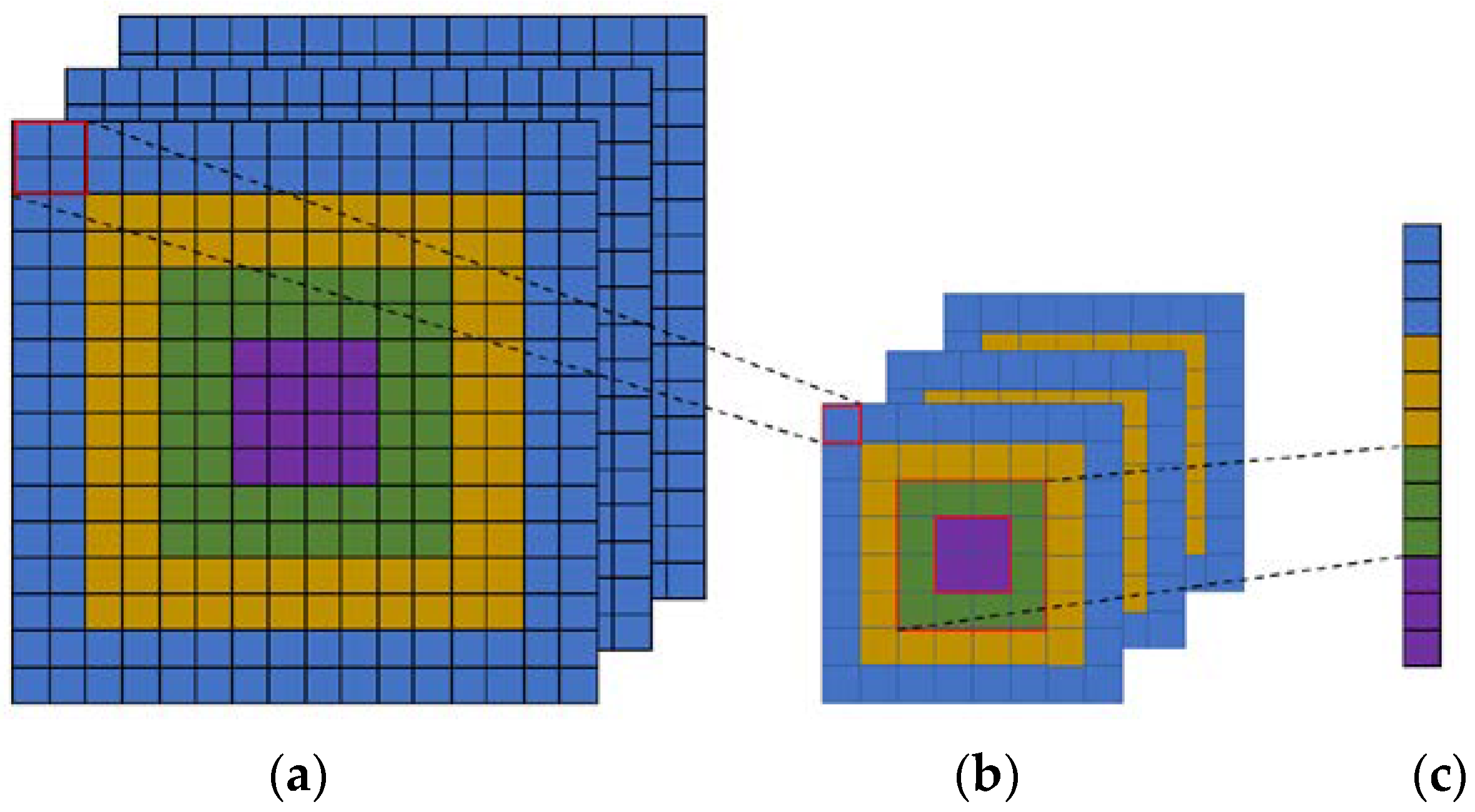
We consider a network with fixed-size input (256 × 256) images. To compute the concentric circle pooling, we can firstly partition the feature maps into several bins and compute the maximal or average values (corresponding to the max pooling and average pooling methods) for each bin. As shown in Figure 5, we assume that the feature maps after last convolutional layer have a size of () (Figure 5a). With an -level () concentric circle, we adopt a sliding window pooling where the window size and stride is () with denoting the ceiling operation. In the sliding window pooling, the “same” padding operation is used. We can obtain a new feature map that has a size of (), where (Figure 5b). Then, we can efficiently compute the maximum or mean of each annular subregion and obtain representations, where () (Figure 5c). The next fully-connected layer will concatenate these outputs. Here, may not be equal to for the ceiling operation. Therefore, the outputs of the CCP layer are , where .
3. Experiments and Analysis
In this section, we provide the experimental setups and discuss the results of the two public datasets. We implement our CCP-net using all the pretrained convolutional layers in VGG-VD networks as the feature extractor. Then, a fully-connected layer on the top of the last convolutional layer computes the scores for each defined class using the softmax activate function. Dropout [26] is used on the fully-connected layer for controlling the overfitting while training with SGD. We conducted several groups of experiments to investigate the effectiveness of CCP-net for remote sensing scene classification.
3.1. Experimental Setup
We evaluated our proposed model on two public remote sensing scene datasets, which were:
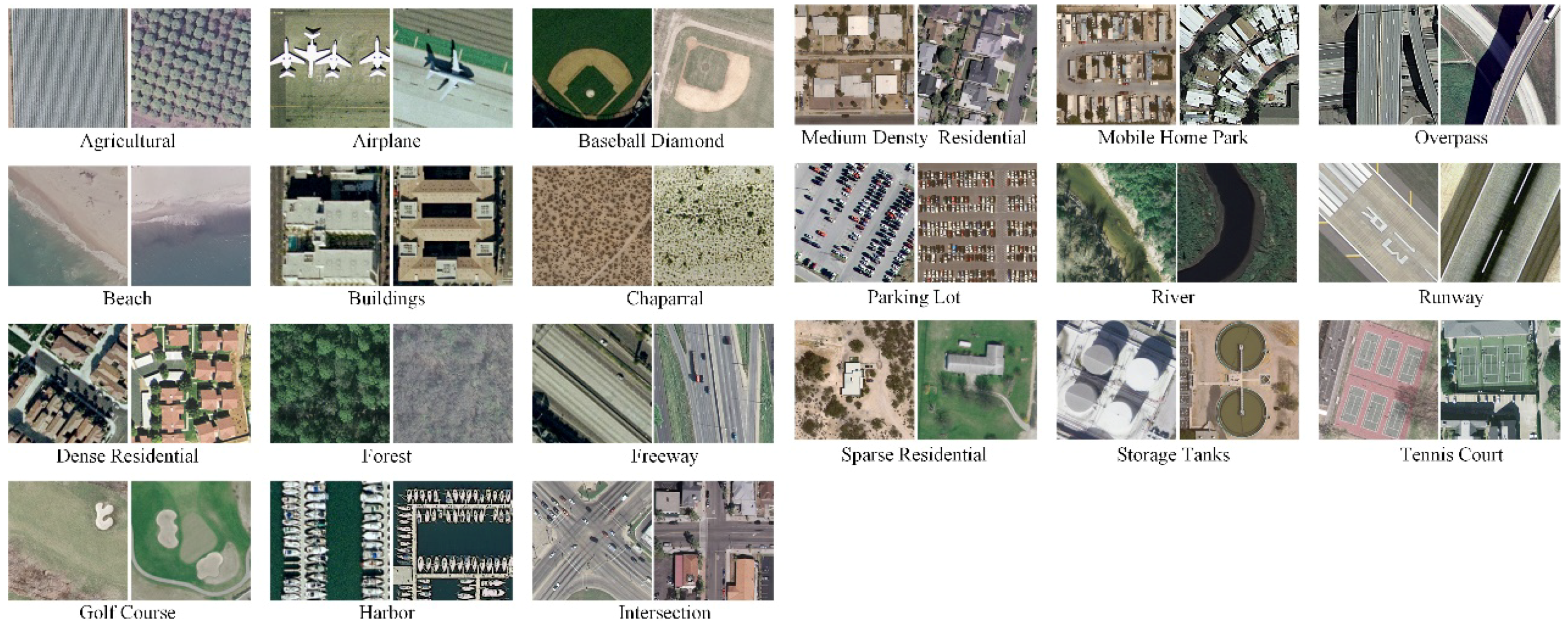
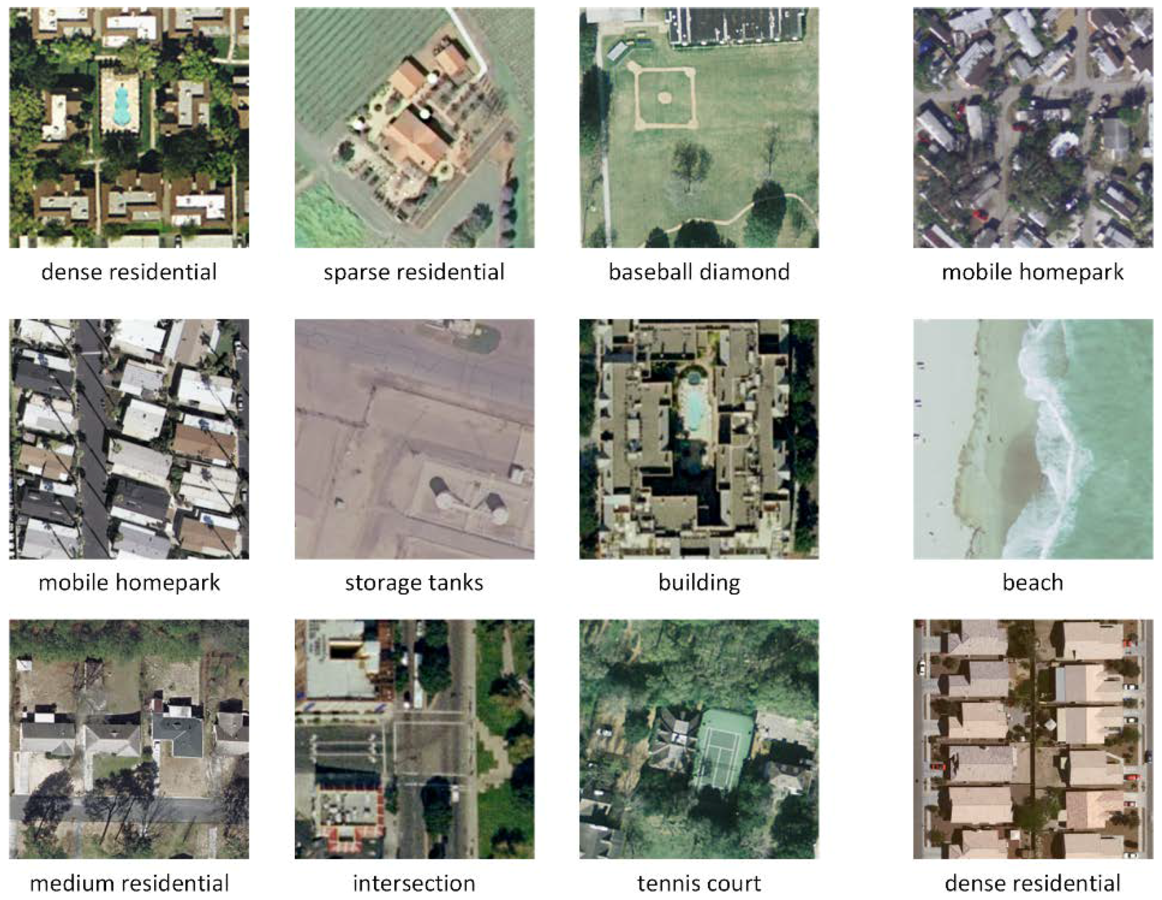
- UC Merced Land Use Dataset. The UC Merced dataset (UCM) is one of the first publicly available high-resolution remote sensing imagery datasets [4]. This dataset contains 21 typical remote sensing scene categories, each of which consists of 100 images measuring pixels with a pixel resolution of 30 cm in the red-green-blue color space. Figure 6 shows two examples of ground truth images from each class in this dataset. The classification of the UCM dataset is challenging because of the high inter-class similarity among categories such as medium residential and dense residential areas.
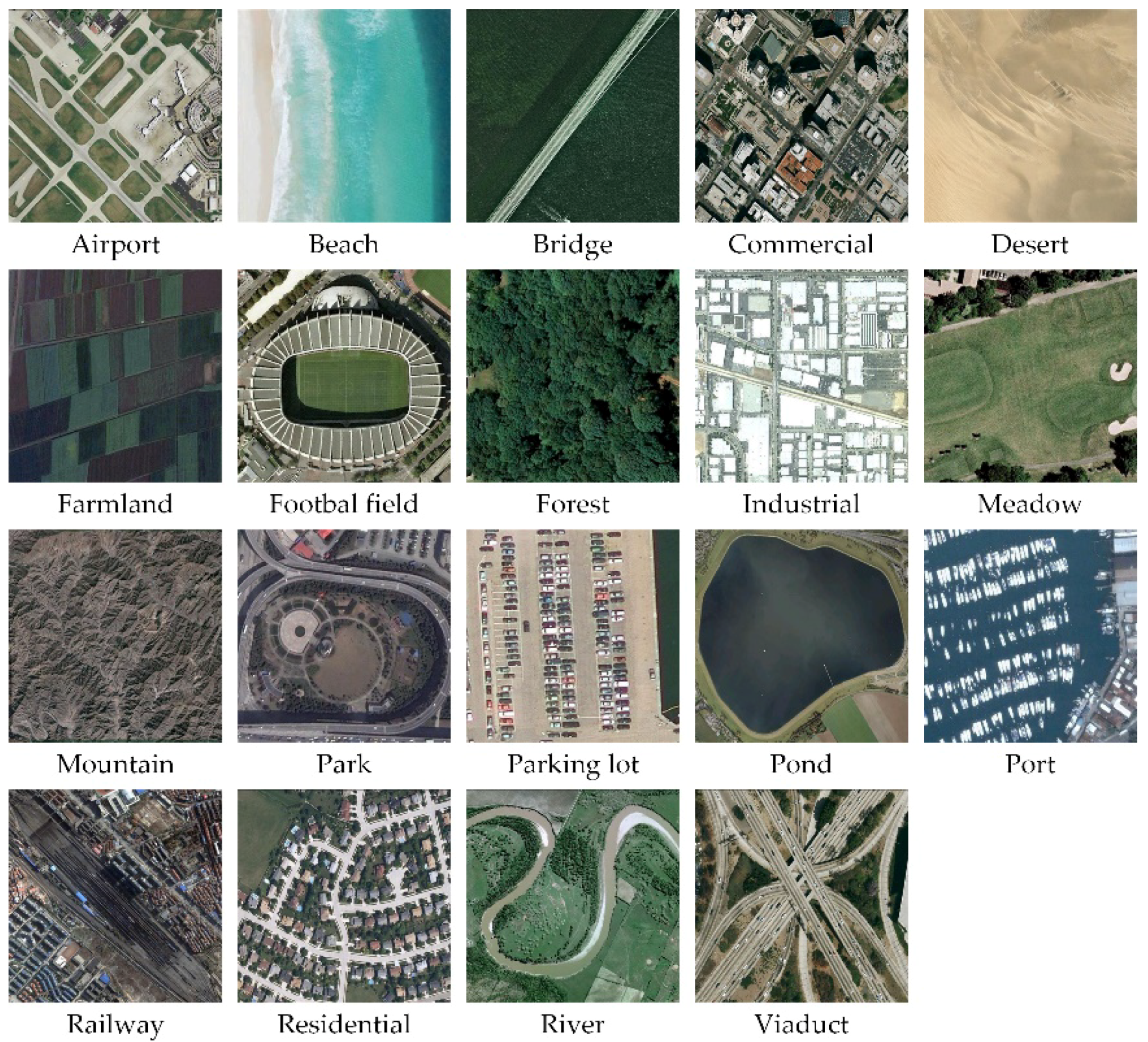
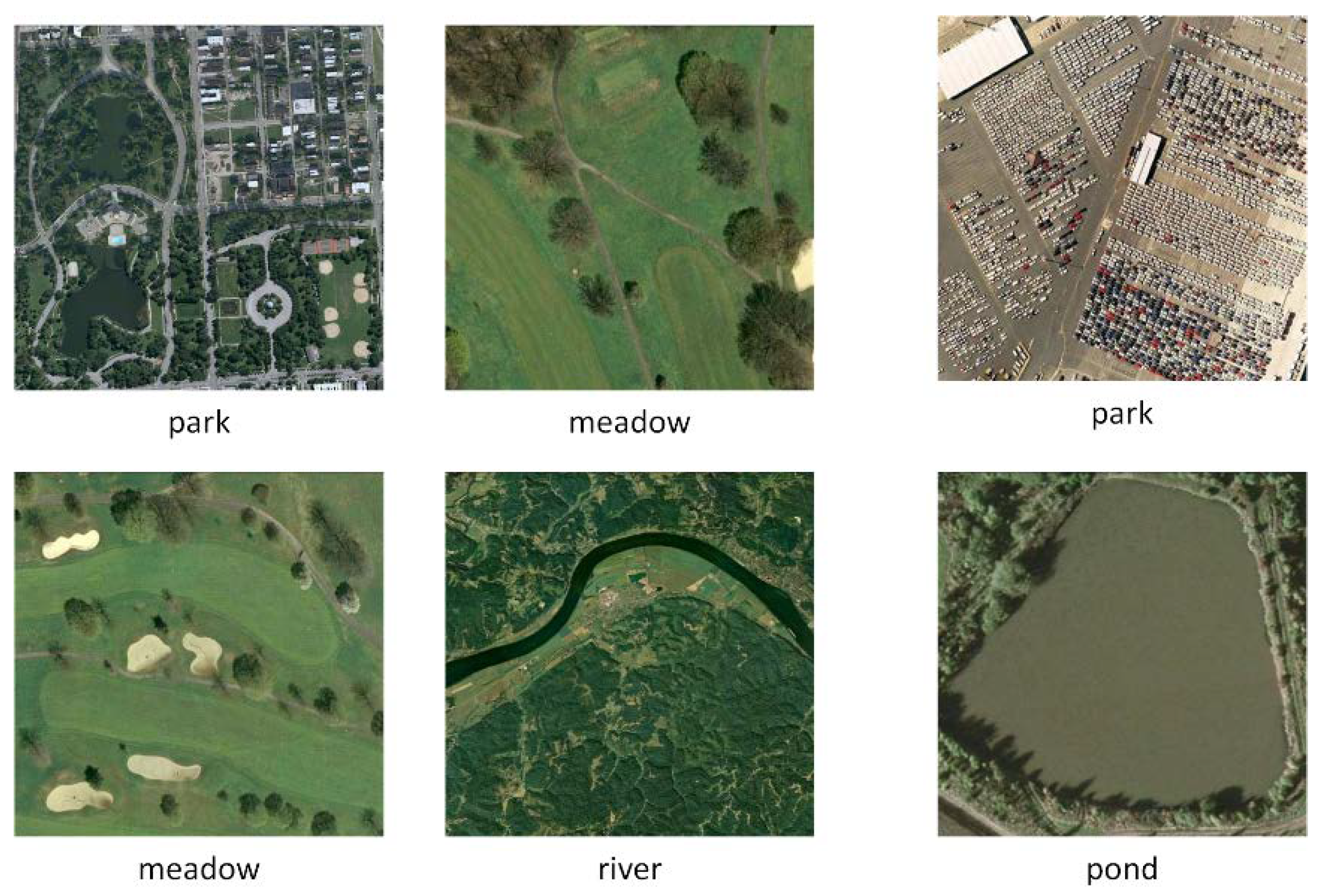
- WHU-RS Dataset. The WHU-RS dataset is a publicly available dataset in which all the images were collected from Google Earth (Google Inc.) [5]. This dataset consists of 950 images with a size of pixels distributed among 19 scene classes. Examples of ground truth images are shown in Figure 7. As compared to the UCM dataset, the scene categories in the WHU-RS dataset are more complicated due to the variation in scale, resolution, and viewpoint-dependent appearance.
We randomly selected samples of each class for training the CNNs and the left rest for testing. The sampling setting as in References [4,36,55] for the two datasets is as follows: 80 training samples per class for the UCM dataset and 30 training samples per class for the WHU-RS dataset. These two datasets were divided 10 times, each run with randomly selected training and testing samples, to obtain reliable results. The classification accuracy rate for the categories was recorded as the mean and standard deviation of 10 runs. We used a high-level neural network named API Keras [56] which was running on top of Tensorflow [57] to implement our network using the CCP layer. Keras Visualization Toolkit [58] was introduced as a high-level toolkit for visualizing the trained Keras neural net models. Experiments in this work were implemented using PyCharm 2017.3/Windows 10 and run on a workstation equipped with a single NVIDIA GeForce GTX 1080 Ti 12 GB GPU.
3.2. Parameter Sensitivity Analysis
3.2.1. Baseline Network Architectures
As with the other pooling method, the CCP is independent of the convolutional network architectures used. The coarsest concentric circle level which has a single annular region is a “global pooling” operation [59]. We investigated the VGG-VD network architectures and showed that CCP improves the accuracy of these architectures. Because fewer layers are suitable for small datasets, we used the pooling layer after the last convolutional layer with a softmax layer following it. We used the original image size for the UCM and WHU-RS datasets. The last convolutional layer generates feature maps with a 21-way softmax layer following it for the UCM dataset, and 37 feature maps with a 19-way softmax layer following it for the WHU-RS dataset. The baseline network architectures with different pooling methods are as follows: global pooling and spatial pyramid pooling. The global pooling layer generates feature maps and the spatial pyramid pooling generates {, }, {, , }, and {, , , } feature maps for 2-level, 3-level, and 4-level pyramids respectively.
3.2.2. Parameter Evaluation
In the HRS images, remote sensing scenes show great variation in shape and scale, thus, the circle number is critical for the effective representation of complex scenes. To quantitatively evaluate the effect of the circle number, we tested different circle numbers from 1 to 8. In these experiments, we trained 100 epochs for these networks. For the training speed, we froze all the convolutional layers and set the initial learning rate to 1 × 10⁻⁴.
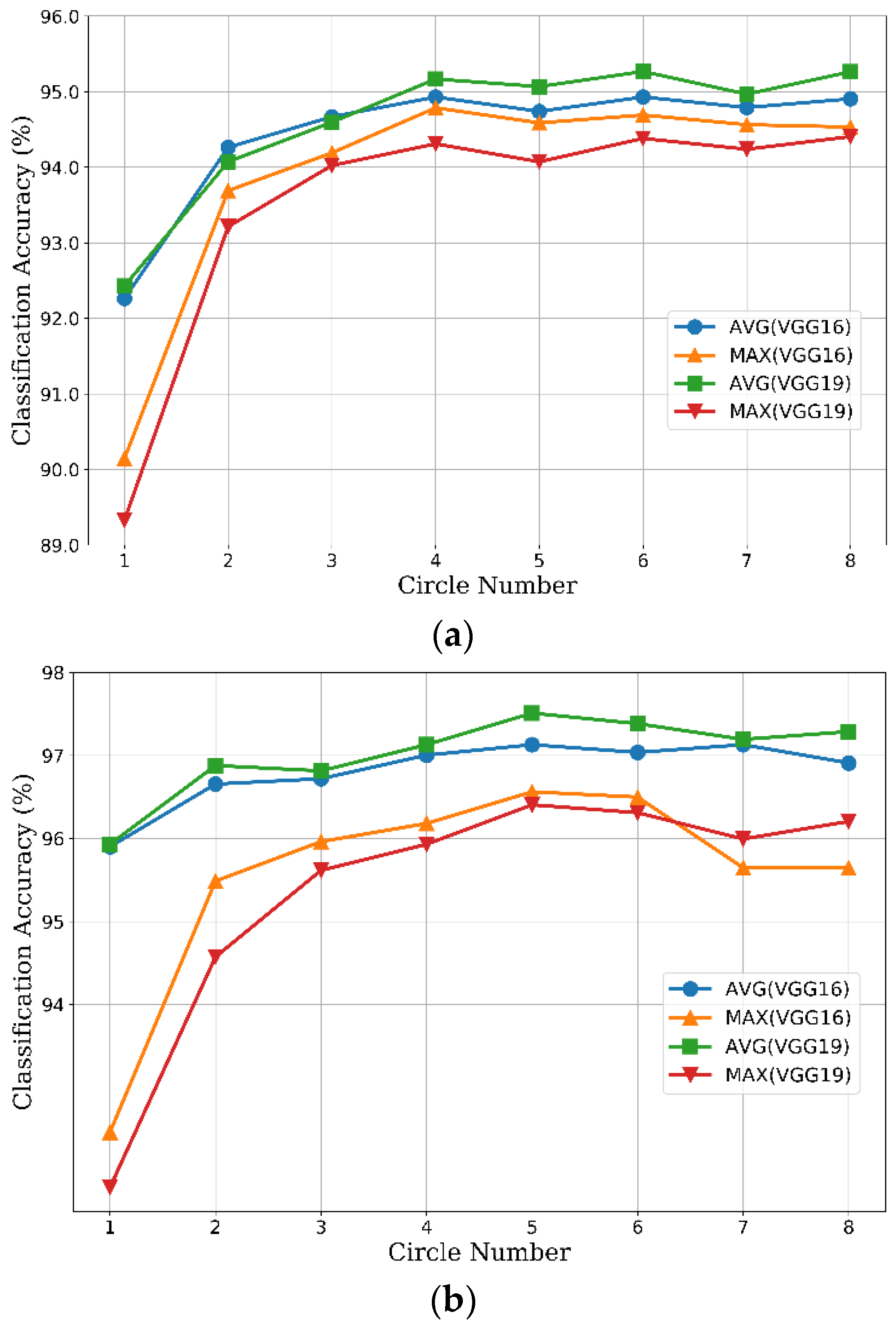
Figure 8 shows the results of CCP-net with different circle numbers and aggregating methods (max pooling and average pooling methods) on the UCM and WHU-RS datasets. In these networks, the convolutional layers have the same structures as the baseline models, whereas the pooling layer after the final convolutional layer is replaced with the CCP layer. Our results in Figure 8 show considerable improvement over the global pooling baselines (the classification accuracy obtained by using only one concentric circle). For the UCM dataset (Figure 8a), the classification accuracies improved gradually with an increase in the circle number, and up to a relative saturation point at 4. The accuracies fluctuate narrowly while the circle number is greater than 4. On the one hand, the outputs of the CCP layer are equal when the circle numbers are between 4 and 7 for the ceiling operation interpreting in Section 2.2. On the other hand, the gap between 4 and 8 is small because the rotation-invariant information is saturated while the circle number is 4. The optimal performance of CCP-net with VGG-VD19 is slightly better than the CCP-net with VGG-VD16. In Figure 8b, we can see that the optimal circle number is 5 for each model on the WHU-RS dataset. Generally, the average pooling method is prior to the max pooling method for each VGG-VD model. For the average pooling method, the accuracies of VGG-VD19 are slightly higher than VGG-VD16, but more time-consuming due to the deeper layer structure. Therefore, we chosen the VGG-VD16 with average pooling method in the following sections for our CCP-net.
We compare our concentric circle pooling with spatial pyramid pooling in Table 1. For the SPP-net, the optimal pyramid for VGG-VD16 is a 4-level pyramid: {, , , }; and for VGG-VD19, it is a 3-level pyramid: {, , }. We can see that the classification accuracies of CPP-net are all better than the SPP-net. The results show that spatial arrangement using regular grid is insufficient for arbitrary oriented objects in remote sensing scene. In Table 1, we also list the results of traditional VGG-VD networks in References [36] which removes the last fully-connected layer (the softmax layer) of a pre-trained CNN and fixes the rest of CNN. The CCP-net perform better than the traditional VGG-VD networks on these two datasets. Overall, the CCP-net considering the rotation-invariant information is effective for remote sensing scene classification tasks.
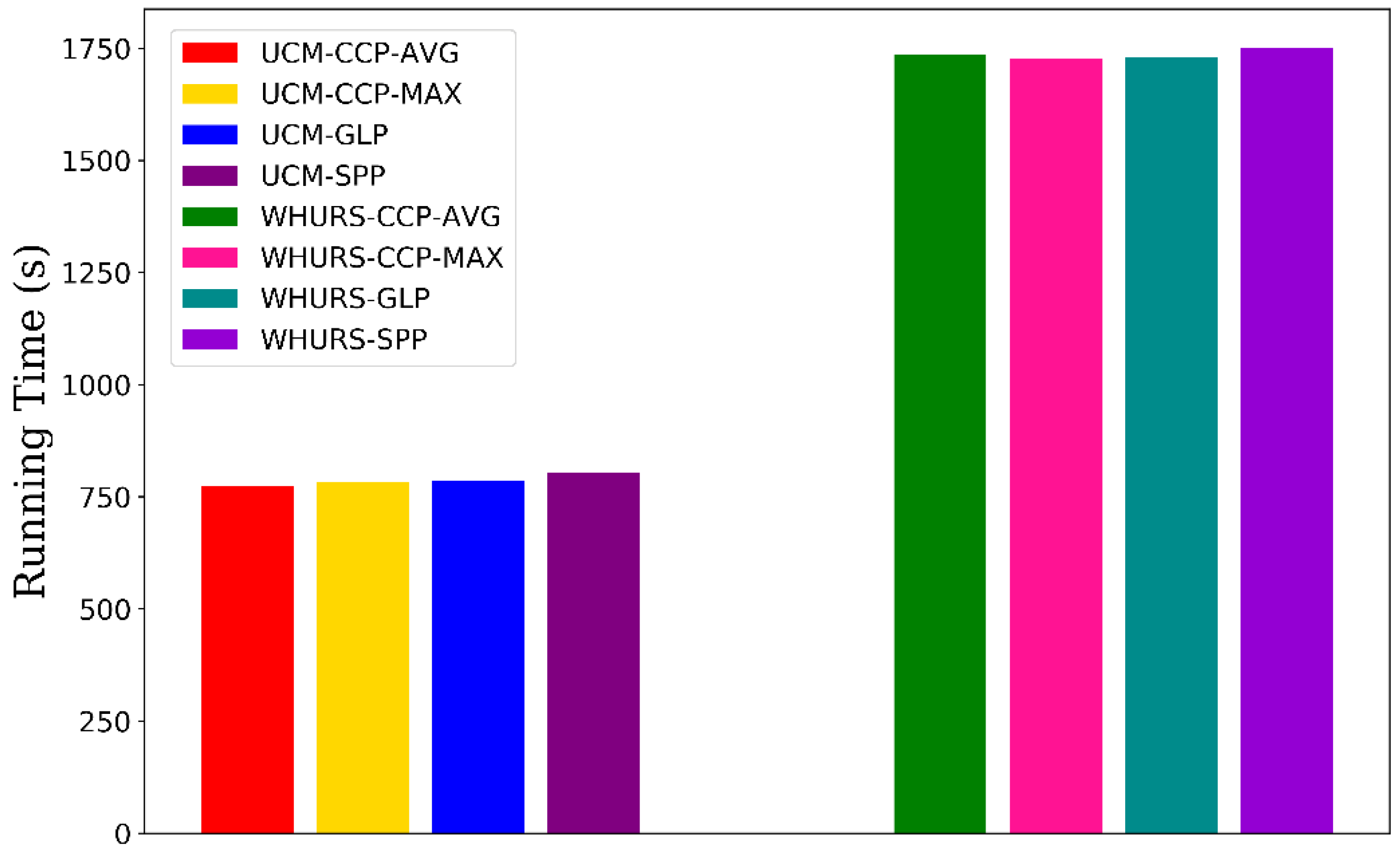
We evaluate the time consumption (measured in terms of seconds) of training models with different pooling methods on the UCM and WHU-RS datasets, shown in Figure 9. These models have almost the same computational cost on the same dataset. Because the length of features after CCP layer is smaller than SPP layer, the CCP-net lead to slightly less time consumption than SPP-net.
3.3. Confusion Matrix
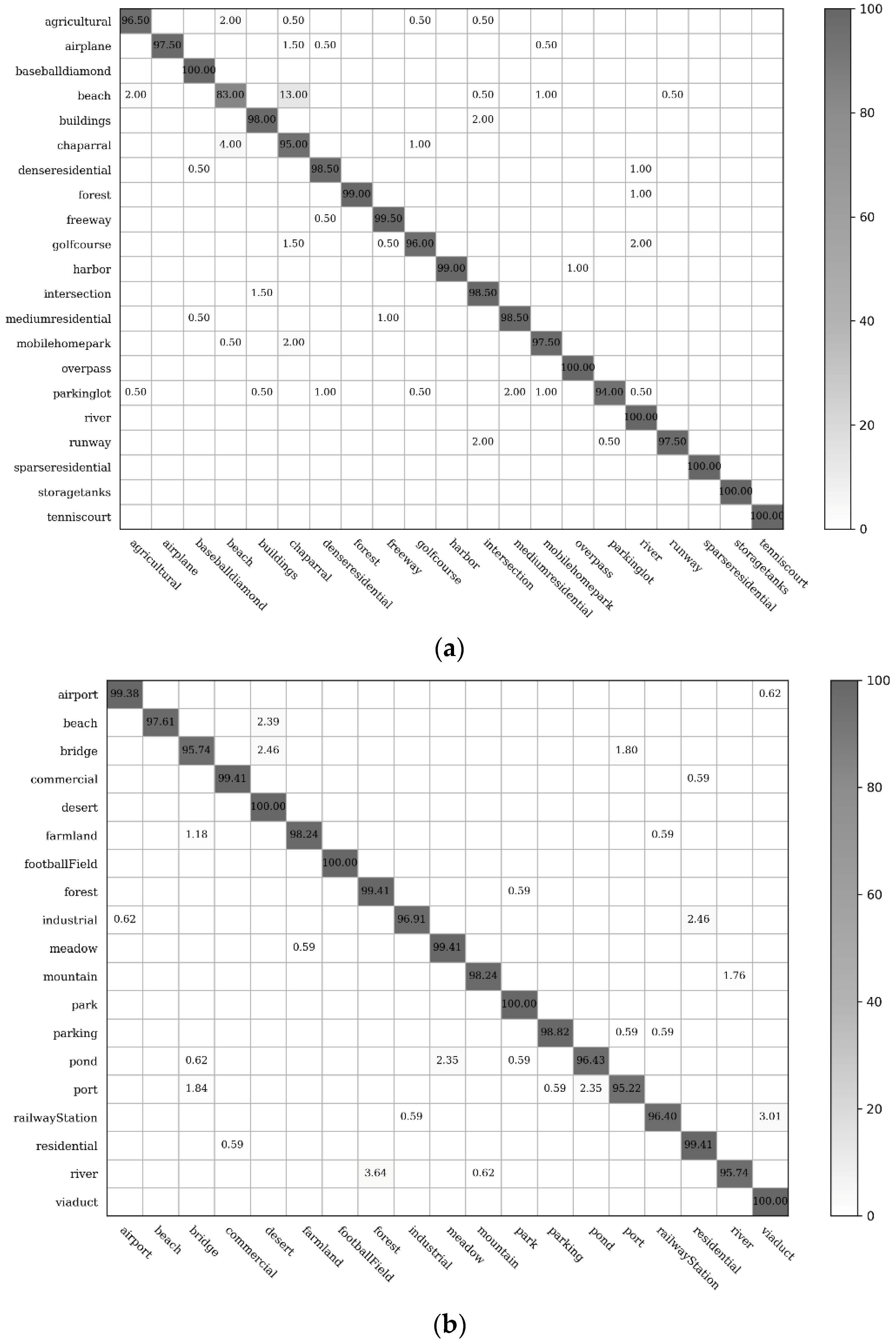
To obtain the optimal performance in CCP-net, we used the VGG-VD16 model and unfroze all the layers to train the entire network. We trained 1000 epochs with a small learning rate equal to 5 × 10⁻⁶. Early stopping [60] was used to stop the training before the weights have converged for controlling overfitting while training with SGD. The classification accuracies (%) of the individual classes on the UCM and WHU-RS datasets using the CCP-net with an optimal circle count as previously described are shown in Figure 9. As shown in these confusion matrices, our proposed method can extract meaningful information for different categories in these two datasets.
In Figure 10, there are 19 among the 21 UCM remote sensing scene classes that have classification accuracies exceeding 95%; the classification accuracies of the baseball diamond, forest, freeway, harbor, overpass, river, sparse residential, storage tank, and tennis court can exceed 99%. The error rates of these easily confused classes, dense residentials, medium residentials, and sparse residentials, are all reduced under 2% for the rotation-invariant spatial arrangements captured by concentric circle pooling. The classification values of 9 among the 19 remote sensing scene categories in the WHU-RS dataset were over 99%. The most confused scene classes are the beach and chaparral in the UCM dataset, and river and forest in the WHU-RS dataset. This is likely to result from the insufficiency of spatial arrangement information and the high similarity of these scene pairs in the aspect of texture structure.
3.4. Comparision with State-of-the-Art Methods
To illustrate the effectiveness of the CCP-net, we compared our results with various state-of-the-art methods that have reported classification accuracies on the UCM dataset. As shown in Table 2, our CCP-net largely outperforms methods that use a sophisticated learning strategy with low-level hand-engineered feature and non-linear classifiers, such as these SIFT-based BOVW and its extension forms like SPM [21] and Spatial Pyramid Co-occurrence Kernel (SPCK++) [4]. Furthermore, Unsupervised Feature Learning methods (UFLs) [7] and their Saliency-Guided version SG + UFL [8] were also involved in the comparison. The results show that our proposed method outperforms these methods, even the well-designed deep learning framework, GoogleLeNet + Fine-tune approach [59], in the terms of classification accuracy. On the WHU-RS dataset, our method achieved considerably better performance (98.23 ± 0.40%) than the MS-CLBP + FV method (94.32 ± 1.2%) [61] and the SIFT + LTP-HF + Color Histogram (93.6%) [55]. The classification accuracies of our CCP-net are slightly inferior to MDDC (98.27 ± 0.53) [39] and the method (98.64%) presented in Reference [36]. These two methods extract features from the convolutional layers of a pre-trained CNN and use a simple linear classifier to train and test. This method can achieve high performance with a small number of training samples. However, our method is more straightforward and end-to-end trainable. The performance of the proposed method is greater than these two methods while the amount of data increases. Overall, CCP-net can obtain remarkable classification results on the public benchmark. The results indicate that our proposed model has great potential for the representation and classification of remote sensing scene images.
4. Discussion
Extensive experiments show that our CCP-net is simple but very effective for remote sensing scene classification in HRS images. We use the concentric circle pooling to capture the rotation-invariant spatial information for the CNN architectures. We create a rotated dataset based on the UCM dataset with each image randomly rotated. Thus, each class includes 200 images in the rotated dataset.
In Table 3 we compare the CCP-net and SPP-net on the UCM and the rotated datasets. We froze all the convolutional layers and set the initial learning rate to 1 × 10⁻⁴. These networks use the optimal parameters obtained in Section 3.2.2. For these two networks, the overall classification accuracies on the rotated dataset are greater than the results on the UCM dataset. This may be because the rotated dataset contains additional rotated images based on the UCM dataset, which makes the sample images more abundant. For the additional rotated images, the CCP-net has more advantage over the SPP-net in the classification accuracy. This proves that the CCP-net are insensitive to the rotation of remote sensing scenes. The performance of CCP-net in almost all categories are improved more than SPP-net. The classification accuracies of some categories in the SPP-net are decreased more than 1%. The possible reason is that some of the classes are similar in part of scene image and the rotated images will increase their similarity. For example, the freeway and overpass are more easily to be confused, and the forest are more easily to be recognized as sparse residential. This is an indication of the importance of rotation-invariance for the remote sensing scene images. Compare with the results on the UCM dataset, the classification accuracies on the rotated dataset are 1.7% higher for CCP-net and 0.74% higher for SPP-net. The promotion of CCP-net is more than twice that of SPP-net. To sum up, our proposed method is rotation-invariant to image scenes and is effective for remote sensing scene image classification.
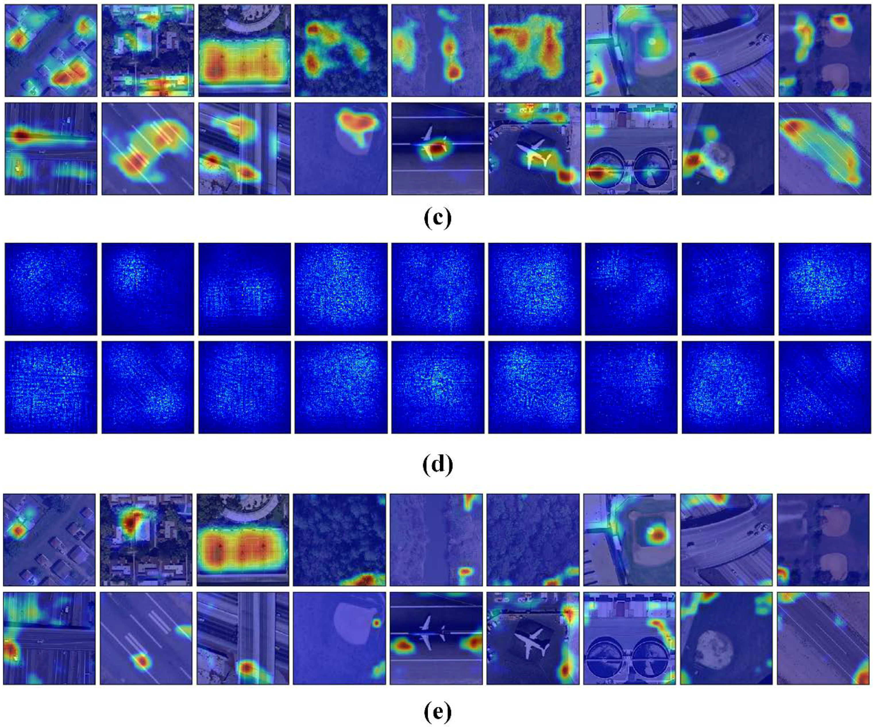
We use attention heatmap and gradient-weighted class activation maps [57] to assess whether a network is attending to correct parts of the image to generate a decision. The entire models were trained as Section 3.3 to fine-tune the convolutional layers that transfer from VGG-VD16. Figure 11 show the visualization results of CCP-net and SPP-net on the UCM dataset. In Figure 11b,d, the heatmap images indicate that the edges and corners in the scene images are contribute minimizing the weighted losses the most for these two methods. The saliency regions in the heatmaps of CCP-net are relatively concentrated for the concentric circle pooling in CCP-net. Due to the multiple pyramid-level pooling, the SPP-net may pay attention to more regions, especially for the categories with flat and similar pattern, e.g., forest and river. In Figure 11c,e, we show the gradient based class activation maps to produce a coarse localization map of the important regions in the image for CCP-net and SPP-net. These maps use the class-specific gradient information flowing into the final convolutional layer of CNNs. It is shown that these networks can learn meaningful representation for scene classification, e.g., tennis courts and baseball diamond. Owing to the rotation invariance, the CCP-net can take notice of the distinguishing parts in scene images, for example, intersection part in the overpass, and airplane in the airport. This illustrates that the rotation invariance can help the CNNs to follow the discriminative parts between remote sensing scene categories.
Several example images are presented in Figure 12 and Figure 13 that compare results from the networks with concentric circle pooling and spatial pyramid pooling on the UCM and WHU-RS datasets. As shown in Figure 12, these remote sensing scene images containing small objects, like the baseball diamond and storage tank, can be recognized by our CCP-net model. These remote sensing scenes are easily misclassified using SPP-net; the occurrences of small objects in different subregions, such as the baseball diamond, are recognized incorrectly as a golf course. Due to the rotation-invariant information, our model is more robust with respect to clutter background, like tennis courts in Figure 8 and parks in Figure 13. SPP-net, however, is more suitable for the scene images with regular grid layouts, like mobile home parks and beaches in Figure 12 and parks in Figure 13. Overall, CCP-net outperform SPP-net in classification accuracy because the remote sensing scene images are orthographical and irregular. The rotation-invariant is more import than the regular spatial arrangement for the remote sensing scene classification tasks.
These experimental results demonstrate the importance of rotation-invariant information for deep CNN features for remote sensing scene datasets. Our proposed concentric circle pooling method can assist the CNNs to be insensitive to the rotation of scenes and localize class-discriminative regions, thus, improve classification accuracies for remote sensing scene images.
5. Conclusions
Concentric circle pooling is a simple but effective solution for handling rotation-invariance problems. This issue is important in remote sensing scene classification using CNN architectures. We have suggested a solution to train a deep network with a concentric circle pooling layer. The resulting CCP-net outstanding accuracy is greater than for the global pooling and spatial pyramid pooling methods in the scene classification tasks. The CCP-net is evaluated using two publicly available ground truth image datasets. The experimental results prove that the proposed method delivers a competitive performance in the classification accuracy against state-of-the-art methods. In future studies, we plan to investigate a solution to handle the different input sizes and multiple scales for the CCP layer and evaluate the performance on big datasets such as NWPU-resisc45 [29].
Author Contributions
K.Q. proposed the algorithm and performed the experiments under the supervision of Q.G. C.Y., F.P., S.S. and H.W. contributed to discuss and analysis the experimental results. K.Q. drafted the manuscript, which was revised by all authors. All authors read and approved the submitted manuscript.
Funding
This work was supported by the National Key R&D Program of China under Grant No. 2017YFB0503704, National Natural Science Foundation of China under Grant No. 41701410, China Postdoctoral Science Foundation under Grant No. 2017M622550, and Open Research Fund of State Key Laboratory of Information Engineering in Surveying, Mapping and Remote Sensing under Grant No. 16R02.
Acknowledgments
The authors would like to thank the editors and the anonymous reviewers for their comments and suggestions.
Conflicts of Interest
The authors declare no conflict of interest.
References
- Zhou, W.; Troy, A. An object-oriented approach for analysing and characterizing urban landscape at the parcel level. Int. J. Remote Sens. 2008, 29, 3119–3135. [Google Scholar] [CrossRef]
- Zhang, H.; Lin, H.; Li, Y.; Zhang, Y. Feature extraction for high-resolution imagery based on human visual perception. Int. J. Remote Sens. 2013, 34, 1146–1163. [Google Scholar] [CrossRef]
- Rogan, J.; Chen, D. Remote sensing technology for mapping and monitoring land-cover and land-use change. Prog. Plan. 2004, 61, 301–325. [Google Scholar] [CrossRef]
- Yang, Y.; Newsam, S. Bag-of-visual-words and spatial extensions for land-use classification. In Proceedings of the 18th SIGSPATIAL International Conference on Advances in Geographic Information Systems, San Jose, CA, USA, 2–5 November 2010; pp. 270–279. [Google Scholar]
- Xia, G.S.; Yang, W.; Delon, J.; Gousseau, Y.; Sun, H.; Maitre, H. Structrual High-Resolution Satellite Image Indexing. In Proceedings of the ISPRS, TC VII Symposium Part A: 100 Years ISPRS—Advancing Remote Sensing Science, Vienna, Austria, 5–7 July 2010. [Google Scholar]
- Cheng, G.; Han, J.; Zhou, P.; Guo, L. Multi-class geospatial object detection and geographic image classification based on collection of part detectors. ISPRS J. Photogramm. Remote Sens. 2014, 98, 119–132. [Google Scholar] [CrossRef]
- Cheriyadat, A. Unsupervised Feature Learning for Aerial Scene Classification. IEEE Trans. Geosci. Remote Sens. 2014, 52, 439–451. [Google Scholar] [CrossRef]
- Zhang, F.; Du, B.; Zhang, L. Saliency-Guided Unsupervised Feature Learning for Scene Classification. IEEE Trans. Geosci. Remote Sens. 2015, 53, 2175–2184. [Google Scholar] [CrossRef]
- Fan, J.; Tan, H.L.; Lu, S. Multipath sparse coding for scene classification in very high resolution satellite imagery. SPIE Remote Sens. 2015, 9643. [Google Scholar] [CrossRef]
- Hu, F.; Xia, G.; Wang, Z.; Huang, X.; Zhang, L.; Sun, H. Unsupervised Feature Learning via Spectral Clustering of Multidimensional Patches for Remotely Sensed Scene Classification. IEEE J. Sel. Top. Appl. Earth Obs. Remote Sens. 2015, 8, 2015–2030. [Google Scholar] [CrossRef]
- Zhao, L.J.; Tang, P.; Huo, L.Z. Land-use scene classification using a concentric circle-structured multiscale bag-of-visual-words model. IEEE J. Sel. Top. Appl. Earth Obs. Remote Sens. 2014, 7, 4620–4631. [Google Scholar] [CrossRef]
- Chehdi, K.; Soltani, M.; Cariou, C. Pixel classification of large-size hyperspectral images by affinity propagation. J. Appl. Remote Sens. 2014, 8, 083567. [Google Scholar] [CrossRef] [Green Version]
- Yu, Q. Object-based detailed vegetation classification with airborne high spatial resolution remote sensing imagery. Photogramm. Eng. Remote Sens. 2006, 72, 799–811. [Google Scholar] [CrossRef]
- Zhao, Y.; Zhang, L.; Li, P.; Huang, B. Classification of high spatial resolution imagery using improved gaussian markov random-field-based texture features. IEEE Trans. Geosci. Remote Sens. 2007, 45, 1458–1468. [Google Scholar] [CrossRef]
- Sivic, J.; Zisserman, A. Video Google: A text retrieval approach to object matching in videos. In Proceedings of the IEEE International Conference on Computer Vision, Nice, France, 13–16 October 2003; pp. 1470–1477. [Google Scholar]
- Csurka, G.; Dance, C.R.; Fan, L.; Willamowski, J.; Bray, C. Visual categorization with bags of keypoints. In Proceedings of the Workshop on Statistical Learning in Computer Vision, European Conference on Computer Vision, Prague, Czech Republic, 11–14 May 2004; pp. 1–22. [Google Scholar]
- Bosch, A.; Zisserman, A.; Muoz, X. Scene classification using a hybrid generative/discriminative approach. IEEE Trans. Pattern Anal. Mach. Intell. 2008, 30, 712–727. [Google Scholar] [CrossRef] [PubMed]
- Jegou, H.; Douze, M.; Schmid, C. Improving bag-of-features for large scale image search. Int. J. Comput. Vis. 2010, 87, 316–336. [Google Scholar] [CrossRef] [Green Version]
- Lowe, D.G. Distinctive image features from scale-invariant keypoints. Int. J. Comput. Vis. 2004, 60, 91–110. [Google Scholar] [CrossRef]
- Dalal, N.; Triggs, B. Histograms of oriented gradients for human detection. In Proceedings of the IEEE Computer Society Conference on Computer Vision and Pattern Recognition, San Diego, CA, USA, 20–25 June 2005; pp. 886–893. [Google Scholar]
- Lazebnik, S.; Schmid, C.; Ponce, J. Beyond bags of features: Spatial pyramid matching for recognizing natural scene categories. In Proceedings of the IEEE Conference on Computer Vision and Pattern Recognition, New York, NY, USA, 17–22 June 2006; pp. 2169–2178. [Google Scholar]
- Qi, K.; Wu, H.; Shen, C.; Gong, J. Land-use scene classification in high-resolution remote sensing images using improved correlatons. IEEE Geosci. Remote Sens. Lett. 2015, 12, 2403–2407. [Google Scholar] [CrossRef]
- Chen, S.; Tian, Y. Pyramid of Spatial Relations for Scene-Level Land Use Classification. IEEE Trans. Geosci. Remote Sens. 2015, 53, 1947–1957. [Google Scholar] [CrossRef]
- Chen, X.; Xiang, S.; Liu, C.L.; Pan, C.H. Vehicle detection in satellite images by hybrid deep convolutional neural networks. IEEE Geosci. Remote Sens. Lett. 2017, 11, 1797–1801. [Google Scholar] [CrossRef]
- Zhao, W.; Du, S. Scene classification using multi-scale deeply described visual words. Int. J. Remote Sens. 2016, 37, 4119–4131. [Google Scholar] [CrossRef]
- Krizhevsky, A.; Sutskever, I.; Hinton, G.E. Imagenet classification with deep convolutional neural networks. In Proceedings of the Twenty-Sixth Annual Conference on Neural Information Processing Systems, Lake Tahoe, NY, USA, 3–8 December 2012; pp. 1097–1105. [Google Scholar]
- Girshick, R.; Donahue, J.; Darrell, T.; Malik, J. Rich feature hierarchies for accurate object detection and semantic segmentation. In Proceedings of the IEEE Conference on Computer Vision and Pattern Recognition, Columbus, OH, USA, 23–28 June 2014; pp. 580–587. [Google Scholar]
- Hariharan, B.; Arbelaez, P.; Girshick, R.; Malik, J. Simultaneous detection and segmentation. In Proceedings of the European Conference on Computer Vision, Zurich, Switzerland, 6–12 September 2014; pp. 297–312. [Google Scholar]
- Cheng, G.; Han, J.; Lu, X. Remote sensing image scene classification: Benchmark and state of the art. In Proc. IEEE 2017, 105, 1865–1883. [Google Scholar] [CrossRef]
- Cimpoi, M.; Maji, S.; Kokkinos, I.; Vedaldi, A. Deep filter banks for texture recognition, description, and segmentation. Int. J. Comput. Vis. 2016, 118, 65–94. [Google Scholar] [CrossRef] [PubMed]
- Penatti, O.A.; Nogueira, K.; dos Santos, J.A. Do Deep Features Generalize from Everyday Objects to Remote Sensing and Aerial Scenes Domains? In Proceedings of the IEEE Conference on Computer Vision and Pattern Recognition Workshops, Boston, MA, USA, 7–12 June 2015; pp. 44–51. [Google Scholar]
- Chatfield, K.; Simonyan, K.; Vedaldi, A.; Zisserman, A. Return of the Devil in the Details: Delving Deep into Convolutional Nets. In Proceedings of the British Machine Vision Conference, Nottingham, UK, 1–5 September 2014. [Google Scholar]
- Donahue, J.; Jia, Y.; Vinyals, O.; Hoffman, J.; Zhang, N.; Tzeng, E.; Darrell, T. DeCAF: A Deep Convolutional Activation Feature for Generic Visual Recognition. In Proceedings of the International Conference on Machine Learning, Beijing, China, 21–26 June 2014; pp. 647–655. [Google Scholar]
- Oquab, M.; Bottou, L.; Laptev, I.; Sivic, J. Learning and transferring mid-level image representations using convolutional neural networks. In Proceedings of the IEEE Conference on Computer Vision and Pattern Recognition, Columbus, OH, USA, 23–28 June 2014; pp. 1717–1724. [Google Scholar]
- Zeiler, M.D.; Fergus, R. Visualizing and understanding convolutional networks. In Proceedings of the European Conference on Computer Vision, Zurich, Switzerland, 6–12 September 2014; pp. 818–833. [Google Scholar]
- Hu, F.; Xia, G.; Hu, J.; Zhang, L. Transferring deep convolutional neural networks for the scene classification of high-resolution remote sensing imagery. Remote Sens. 2015, 7, 14680–14707. [Google Scholar] [CrossRef]
- Cheng, G.; Yang, C.; Yao, X.; Guo, L.; Han, J. When deep learning meets metric learning: Remote sensing image scene classification via learning discriminative cnns. IEEE Trans. Geosci. Remote Sens. 2018, 56, 2811–2821. [Google Scholar] [CrossRef]
- Deng, J.; Dong, W.; Socher, R.; Li, L.J.; Li, K.; Fei-Fei, L. Imagenet: A large-scale hierarchical image database. In Proceedings of the IEEE Conference on Computer Vision and Pattern Recognition, Miami, FL, USA, 20–25 June 2009; pp. 248–255. [Google Scholar]
- Qi, K.; Yang, C.; Guan, Q.; Wu, H.; Gong, J. A multiscale deeply described correlatons-based model for land-use scene classification. Remote Sens. 2017, 9, 917. [Google Scholar] [CrossRef]
- Grauman, K.; Darrell, T. The pyramid match kernel: Discriminative classification with sets of image features. In Proceedings of the International Conference on Computer Vision, Beijing, China, 17–21 October 2005; pp. 1458–1465. [Google Scholar]
- He, K.; Zhang, X.; Ren, S.; Sun, J. Spatial pyramid pooling in deep convolutional networks for visual recognition. IEEE Trans. Pattern Anal. Mach. Intell. 2015, 37, 1904–1916. [Google Scholar] [CrossRef] [PubMed]
- Lu, X.; Zheng, X.; Yuan, Y. Remote sensing scene classification by unsupervised representation learning. IEEE Trans. Geosci. Remote Sens. 2017, 55, 5148–5157. [Google Scholar] [CrossRef]
- Battiato, S.; Farinella, G.M.; Gallo, G.; Ravi, D. Spatial hierarchy of textons distributions for scene classification. In Conference on Multimedia Modeling; Springer: Berlin/Heidelberg, Germany, 2009; pp. 333–343. [Google Scholar]
- Zhou, L.; Zhou, Z.; Hu, D. Scene classification using multi-resolution low-level feature combination. Neurocomputing 2013, 122, 284–297. [Google Scholar] [CrossRef]
- Cheng, G.; Zhou, P.; Han, J. Learning rotation-invariant convolutional neural networks for object detection in vhr optical remote sensing images. IEEE Trans. Geosci. Remote Sens. 2016, 54, 7405–7415. [Google Scholar] [CrossRef]
- Li, K.; Cheng, G.; Bu, S.; You, X. Rotation-insensitive and context-augmented object detection in remote sensing images. IEEE Trans. Geosci. Remote Sens. 2018, 56, 2337–2348. [Google Scholar] [CrossRef]
- Rao, A.; Srihari, R.K.; Zhang, Z. Spatial color histograms for content-based image retrieval. In Proceedings of the IEEE International Conference on TOOLS with Artificial Intelligence, Chicago, IL, USA, 9–11 November 1999; pp. 183–186. [Google Scholar]
- Lazebnik, S.; Schmid, C.; Ponce, J. A sparse texture representation using local affine regions. IEEE Trans. Pattern Anal. Mach. Intell. 2005, 27, 1265–1278. [Google Scholar] [CrossRef] [PubMed] [Green Version]
- Wang, G.; Wang, X.; Fan, B.; Pan, C. Feature extraction by rotation-invariant matrix representation for object detection in aerial image. IEEE Geosci. Remote Sens. Lett. 2017, 14, 851–855. [Google Scholar] [CrossRef]
- Li, Z.; Song, Y.; Mcloughlin, I.; Dai, L. Compact Convolutional Neural Network Transfer Learning for Small-Scale Image Classification. In Proceedings of the IEEE International Conference on Acoustics, Speech and Signal Processing (ICASSP), Shanghai, China, 20–25 March 2016; pp. 2737–2741. [Google Scholar] [CrossRef]
- LeCun, Y.; Bengio, Y.; Hinton, G. Deep Learning. Nature 2015, 521, 436–444. [Google Scholar] [CrossRef] [PubMed]
- Rumelhart, D.E.; Hintont, G.E.; Williams, R.J. Learning representations by back-propagating errors. Nature 1986, 323, 533–536. [Google Scholar] [CrossRef]
- Simonyan, K.; Zisserman, A. Very deep convolutional networks for large-scale image recognition. In Proceedings of the International Conference on Learning Representations, San Diego, CA, USA, 7–9 May 2015. [Google Scholar]
- Castelluccio, M.; Poggi, G.; Sansone, C.; Verdoliva, L. Land Use Classification in Remote Sensing Images by Convolutional Neural Networks. Available online: http://arxiv.org/abs/1508.00092 (accessed on 30 March 2017).
- Sheng, G.; Yang, W.; Xu, T.; Sun, H. High-resolution satellite scene classification using a sparse coding based multiple feature combination. Int. J. Remote Sens. 2012, 33, 2395–2412. [Google Scholar] [CrossRef]
- Chollet, F. Keras, GitHub Repository. 2015. Available online: https://github.com/fchollet/keras (accessed on 6 September 2017).
- Abadi, M.; Agarwal, A.; Barham, P.; Brevdo, E.; Chen, Z. TensorFlow: Large-Scale Machine Learning on Heterogeneous Systems. 2015. Available online: http://tensorflow.org/ (accessed on 6 September 2017).
- Raghavendra, K. Keras-Vis. 2017. Available online: https://github.com/raghakot/keras-vis. (accessed on 18 February 2018).
- Szegedy, C.; Liu, W.; Jia, Y.; Sermanet, P.; Reed, S.; Anguelov, D.; Erhan, D.; Vanhoucke, V.; Rabinovich, A. Going deeper with convolutions. In Proceedings of the IEEE Conference on Computer Vision and Pattern Recognition Workshops, Boston, MA, USA, 7–12 June 2015. [Google Scholar]
- Prechelt, L. Automatic early stopping using cross validation: Quantifying the criteria. Neural Netw. 1998, 11, 761–767. [Google Scholar] [CrossRef]
- Huang, L.; Chen, C.; Li, W.; Du, Q. Remote sensing image scene classification using multi-scale completed local binary patterns and fisher vectors. Remote Sens. 2016, 8, 483. [Google Scholar] [CrossRef]
- Negrel, R.; Picard, D.; Gosselin, P.H. Evaluation of second-order visual features for land-use classification. In Proceedings of the International Workshop on Content-Based Multimedia Indexing, Klagenfurt, Austria, 18–20 June 2014; pp. 1–5. [Google Scholar]
- Qi, K.; Liu, W.; Yang, C.; Guan, Q.; Wu, H. Multi-Task Joint Sparse and Low-Rank Representation for the Scene Classification of High-Resolution Remote Sensing Image. Remote Sens. 2017, 9, 10. [Google Scholar] [CrossRef]
Figure 1.
The example architecture of remote sensing scene classification using VGG-VD16. It is composed of 13 convolutional layers and 3 fully-connected layers.
Figure 1.
The example architecture of remote sensing scene classification using VGG-VD16. It is composed of 13 convolutional layers and 3 fully-connected layers.

Figure 2.
The rotation variation problem in CNNs for remote sensing scene classification. (a) One channel of feature maps extracting by the last convolutional layer of VGG-VD16 for each image; (b) We flattened each feature map in (a) into one-dimensional representation, split them into four parts, and put each part in different subgraph for visualization. Each row in a subgraph is corresponding to different image in (a).

Figure 3.
The example of the spatial partition of the concentric circle pooling strategy to represent spatial information. (a) The original concentric circle structure-based pooling method; (b) The proposed concentric circle pooling method.
Figure 3.
The example of the spatial partition of the concentric circle pooling strategy to represent spatial information. (a) The original concentric circle structure-based pooling method; (b) The proposed concentric circle pooling method.

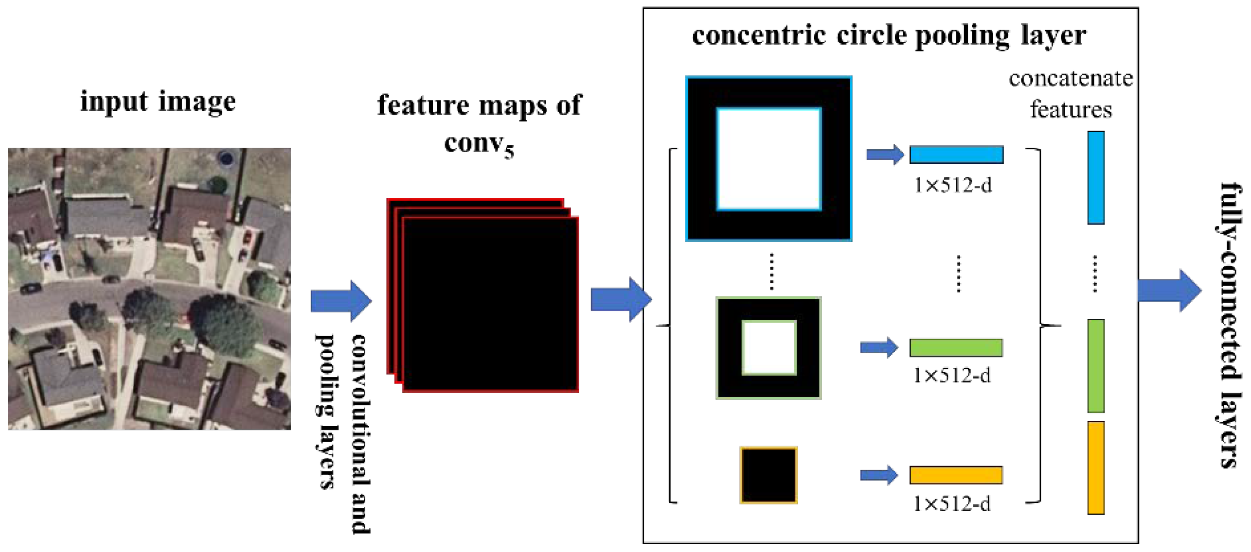
Figure 4.
A network structure with a concentric circle pooling layer. The convolutional and pooling layers except for the last pooling layer in VGG-VD16 are transformed to this network and 512 is the filter number of the conv5 layer, which is the last convolutional layer.
Figure 4.
A network structure with a concentric circle pooling layer. The convolutional and pooling layers except for the last pooling layer in VGG-VD16 are transformed to this network and 512 is the filter number of the conv5 layer, which is the last convolutional layer.

Figure 5.
An example four-level concentric circle pooling. (a) The output feature map of last convolutional layer; (b) The results after sliding window pooling which transforms each circle in output feature map of last convolutional layer to one-pixel width; (c) The outputs of concentric circle pooling which computes the maximum or mean of each annular subregion for each channel and concatenates them.

Figure 6.
Two example ground truth images of each scene category in the UC Merced dataset.

Figure 7.
The example ground truth images of each scene category in the WHU-RS dataset.

Figure 8.
The classification accuracy of concentric circle pooling network as a function of circle number. The AVG and MAX in the labels indicate the average aggregate and max average. (a) The UC Merced dataset; (b) The WHU-RS dataset.
Figure 8.
The classification accuracy of concentric circle pooling network as a function of circle number. The AVG and MAX in the labels indicate the average aggregate and max average. (a) The UC Merced dataset; (b) The WHU-RS dataset.

Figure 9.
The time consumption of training models with different pooling methods on the UCM and WHU-RS datasets. The AVG, MAX, and GLP in the labels indicate the average aggregate, the max aggregate, and the global pooling.
Figure 9.
The time consumption of training models with different pooling methods on the UCM and WHU-RS datasets. The AVG, MAX, and GLP in the labels indicate the average aggregate, the max aggregate, and the global pooling.

Figure 10.
The confusion matrices showing the classification accuracies (%) for the proposed model. (a) Confusion matrix for the UC Merced dataset; (b) Confusion matrix for the WHU-RS dataset.
Figure 10.
The confusion matrices showing the classification accuracies (%) for the proposed model. (a) Confusion matrix for the UC Merced dataset; (b) Confusion matrix for the WHU-RS dataset.

Figure 11.
The attention heatmaps and the gradient based class activation maps to show the important regions of the scene images in the UC Merced dataset. (a) Original scene images; (b,d) are attention heatmaps for CPP-net and SPP-net; (d,e) are gradient based class activation maps for CCP-net and SPP-net.


Figure 12.
Several example images that compare results from CCP-net and SPP-net on the UC Merced dataset. Images, where SPP-net failed, are shown in the first three columns and images where CCP-net failed are shown in the last column.
Figure 12.
Several example images that compare results from CCP-net and SPP-net on the UC Merced dataset. Images, where SPP-net failed, are shown in the first three columns and images where CCP-net failed are shown in the last column.

Figure 13.
Several example images that compare results from CCP-net and SPP-net on the WHU-RS dataset. Images, where SPP-net failed, are shown in the first two columns and images where CCP-net failed are shown in the last column.
Figure 13.
Several example images that compare results from CCP-net and SPP-net on the WHU-RS dataset. Images, where SPP-net failed, are shown in the first two columns and images where CCP-net failed are shown in the last column.


Table 1.
The comparison of the classification accuracy with spatial pyramid pooling network.
| Accuracy (Mean ± std%) | ||||
|---|---|---|---|---|
| UCM | WHU-RS | |||
| VGG-VD16 | VGG-VD19 | VGG-VD16 | VGG-VD19 | |
| CCP-net | 94.93 ± 0.95 | 95.17 ± 0.92 | 97.13 ± 0.78 | 97.51 ± 0.73 |
| 2-level SPP | 93.47 ± 1.26 | 91.93 ± 1.42 | 95.13 ± 1.35 | 94.38 ± 0.77 |
| 3-level SPP | 93.78 ± 1.19 | 93.38 ± 1.46 | 95.11 ± 1.32 | 94.99 ± 1.1 |
| 4-level SPP | 93.81 ± 1.39 | 93.24 ± 1.4 | 95.21 ± 1.44 | 94.81 ± 1.77 |
| Traditional [36] | 94.07 | 93.15 | 94.35 | 94.36 |
Table 2.
The comparison of the classification accuracy (%) on the UC Merced dataset.
| Method | Accuracy (Mean ± std) |
|---|---|
| BOVW [15] | 71.86 |
| SPM [21] | 74.0 |
| SPCK++ [4] | 77.38 |
| UFL [7] | 81.67 ± 1.23 |
| SG+UFL [8] | 82.72 ± 1.18 |
| VLAT [62] | 94.3 |
| MS-CLBP+FV [61] | 93.0 ± 1.2 |
| MTJSLRC [63] | 91.07 ± 0.67 |
| MBVW [25] | 96.14 |
| CaffeNet [31] | 93.42 ± 1.0 |
| OverFeat [31] | 90.91 ± 1.19 |
| MDDC [39] | 96.92 ± 0.57 |
| GoogLeNet + Fine-tune [59] | 97.1 |
| CCP-net | 97.52 ± 0.97 |
Table 3.
The comparison of the CCP-net and SPP-net on the UC Merced and the rotated datasets. For each network, the two rows are the results of the UC Merced and the rotated datasets, respectively.
Table 3.
The comparison of the CCP-net and SPP-net on the UC Merced and the rotated datasets. For each network, the two rows are the results of the UC Merced and the rotated datasets, respectively.
| Method | Acc | Agri | Air | Base | Beach | Build | Chap | Dres | Fore | Free | Golf | Harb | Inter | Mres | Mph | Over | Park | Riv | Run | Sres | Stor | Tenn |
|---|---|---|---|---|---|---|---|---|---|---|---|---|---|---|---|---|---|---|---|---|---|---|
| CCP-net | 94.93 | 98 | 100 | 97.5 | 100 | 88 | 100 | 76 | 100 | 98 | 94 | 100 | 94.5 | 91.5 | 90 | 97.5 | 99 | 93 | 99.5 | 95.5 | 95 | 86.5 |
| 96.63 | 99. | 100. | 99.5 | 99.25 | 90.75 | 100 | 80.25 | 100. | 97.75 | 95.75 | 99.5 | 95.5 | 95.75 | 96.25 | 98.75 | 100 | 97.75 | 100 | 94.75 | 96.25 | 92.5 | |
| SPP-net | 93.81 | 98.5 | 99 | 98 | 100 | 83.5 | 100 | 73 | 100 | 98.25 | 93 | 100 | 88.25 | 88.5 | 92 | 95.5 | 99 | 94 | 100 | 93.5 | 90 | 86 |
| 94.55 | 99 | 99.75 | 98.5 | 99.25 | 84 | 100 | 74 | 98 | 96.75 | 93.25 | 100 | 89.5 | 91.5 | 97.5 | 94.5 | 99.5 | 95.25 | 99.75 | 93.5 | 92.25 | 89.75 |
© 2018 by the authors. Licensee MDPI, Basel, Switzerland. This article is an open access article distributed under the terms and conditions of the Creative Commons Attribution (CC BY) license (http://creativecommons.org/licenses/by/4.0/).
Share and Cite
MDPI and ACS Style
Qi, K.; Guan, Q.; Yang, C.; Peng, F.; Shen, S.; Wu, H. Concentric Circle Pooling in Deep Convolutional Networks for Remote Sensing Scene Classification. Remote Sens. 2018, 10, 934. https://doi.org/10.3390/rs10060934
AMA Style
Qi K, Guan Q, Yang C, Peng F, Shen S, Wu H. Concentric Circle Pooling in Deep Convolutional Networks for Remote Sensing Scene Classification. Remote Sensing. 2018; 10(6):934. https://doi.org/10.3390/rs10060934
Chicago/Turabian StyleQi, Kunlun, Qingfeng Guan, Chao Yang, Feifei Peng, Shengyu Shen, and Huayi Wu. 2018. "Concentric Circle Pooling in Deep Convolutional Networks for Remote Sensing Scene Classification" Remote Sensing 10, no. 6: 934. https://doi.org/10.3390/rs10060934
Note that from the first issue of 2016, this journal uses article numbers instead of page numbers. See further details here.