Improved Joint Sparse Models for Hyperspectral Image Classification Based on a Novel Neighbour Selection Strategy

Abstract

Joint sparse representation has been widely used for hyperspectral image classification in recent years, however, the equal weight assigned to each neighbouring pixel is less realistic, especially for the edge areas, and one fixed scale is not appropriate for the entire image extent. To overcome these problems, we propose an adaptive local neighbour selection strategy suitable for hyperspectral image classification. We also introduce a multi-level joint sparse model based on the proposed adaptive local neighbour selection strategy. This method can generate multiple joint sparse matrices on different levels based on the selected parameters, and the multi-level joint sparse optimization can be performed efficiently by a simultaneous orthogonal matching pursuit algorithm. Tests on three benchmark datasets show that the proposed method is superior to the conventional sparsity representation methods and the popular support vector machines.

1. Introduction

In recent years, remote sensing images have played an important role in many areas, such as surveillance, land-use classification, forest disturbance, and urban planning [1]. How to exploit the information of remotely-sensed images has been a popular research problem for decades. Hyperspectral images (HSI) have attracted a significant amount of attention due to its high spectral resolution and wide spectral range which make it possible to analyse and distinguish various objects with higher accuracy [2].

One of the most important applications of HSI is supervised classification which assigns a specific class to each pixel based on the spectral information [3]. Various techniques have been employed for this task, such as support vector machines (SVM) [4,5,6], random forest (RF) [7], multinomial logistic regression (MLR) [8], and neural networks (NN) [9]. Among these techniques, SVM has shown its effectiveness for HSI classification, especially when dealing with the Hughes phenomenon of very high-dimensional data [4]. Dimensionality reduction methods were developed to deal with the high dimensionality of HSI data and obtained some promising results [6,10,11]. Although these methods have provided some reasonable solutions to the problem, spatial context has not been fully utilized in those conventional classifiers. Without spatial information being involved, the classification map may produce a more noisy appearance and a lower accuracy [12]. During the past decade, many attempts have been made to integrate the spatial context in the classification tasks. Some methods have focused on feature extraction, such as extended morphological profiles [13,14] and attribute profiles [15,16], which improved the classification results by taking the morphological properties into account. Kernel-based methods, such as the one in [17], use a composite kernel to incorporate spectral and spatial properties, and then images are classified by SVM. In addition, multiple feature learning approaches [18,19], which combine different features learned by various methods, are proven to enhance the classification results. Markov random fields (MRF) [20,21] focus on developing classifiers that can preserve the spatial context by formulating a minimization function of spatial and spectral energy, and the result changes when different weights are assigned to spectral and spatial energy terms. All these techniques are able to incorporate spatial and spectral information.

In the last few years, sparse representation (SR) has been a promising tool in solving many image processing problems, such as denoising [22], fusion [23], and image compression [24]. In [25], SR was used to detect the boundary points and outliers from images, which is proven to be very useful for image processing applications. SR assumes that a natural signal can be linearly expressed by a few coefficients from a so-called dictionary [26]. Now SR has been extended to the classification of HSI based on the assumption that the pixels of a class usually lie in a low-dimensional subspace, despite their high-dimensional characteristics [27]. This enables a test pixel with an unknown label to be linearly represented by a few elements, and then the label can be determined after the coefficient vectors are recovered from a training dictionary. Many studies [28,29,30] have provided a promising result for HSI classification based on SR. Moreover, SR can also learn the probability for a decision fusion classifier [31]. It should be noted that the reconstruction work mechanism makes it very efficient, and can easily accommodate new training data by reconstructing the class-specific dictionary (e.g., directly adding the new training data to the dictionary matrix which corresponding to the label class of the training data) without retraining the whole dataset, which is required for other classifiers, such as SVM and MLR. Another advantage of SR compared to other conventional binary classifiers is that it can label the pixels from multiple classes directly. Many studies have been attempted to explore the merits of SR. Cui and Prasad [32] proposed a class-dependent sparse representation classifier which utilized the k-nearest method to select atoms for SR, and they considered the label information by computing the Euclidean distances between the test sample and k-nearest pixels in a class-specific manner. The class-dependent SR can also be extended to a kernelized variant by using a kernel function. Similar work has been done in [33]. In the report of [34], the authors proposed a multi-layer spatial-spectral sparse representation specifically for hyperspectral image classification. The class residual is computed in the first sparse representation layer, and then the sparse coefficients are determined to be updated or not in the next layer based on a class-dependent residual distribution. The multi-layer strategy is implemented sequentially and the selected atoms’ indices are determined by the classes’ rankings within the minimal residuals. The experimental results have demonstrated its superior results when compared to the traditional sparse coding methods.

In order to further exploit the spatial information, a joint sparse model (JSM) has been proposed [28]. For HSI, neighbouring pixels tend to have similar contextual properties and are highly correlated with each other [35]. JSM assumes that pixels constrained by a region scale share a common sparsity pattern, and these pixels can be linearly represented by a few common atoms which are associated with different sparsity coefficients. Based on this assumption, the test pixel can be replaced with its surrounding neighbours in the JSM model to seek a more reliable representation. Recently, JSM has achieved a better performance when compared to pixel-wise SR methods [36]. However, JSM is sensitive to the selected region scale because near-edge areas require a small region scale and smooth areas need a large region scale. Some experiments have shown that, if an oversized area is selected for a specific test pixel, the accuracy tends to decrease [37]. If the scale is too small, then insufficient contextual properties are included; hence, it is difficult to choose an optimal region scale for JSM.

On the other hand, for a given specific area, distinct structures and characteristics, as well as some irrelevant information, will exhibit; however, some pixels with different spectral structures of the test pixel also exist in this region. If a strategy aims to find the most similar pixels to the test pixel and reject the dissimilar neighbouring pixels, information of correlated spatial context should be more representative for classification. Hence, we propose an adaptive neighbour selection strategy which computes the weights based on distances between pixels, with the labels of training data as a priori information. The structural similarity between the central pixel and its neighbours can be exploited in a more sensible way by considering the different contribution of each spectral band. Based on this, a novel joint sparse model-based classification approach, namely ‘adaptive weighted joint sparse model’ (AJSM) is proposed in this paper. Moreover, we propose a novel classification method with a name ‘multi-level joint sparse representation model’ (MLSR), in order to take advantage of the correlations among neighbouring pixels in a region. The procedures of MLSR are summarized as: (1) Local matrices are obtained by the proposed adaptive neighbour selection strategy. Different thresholds of distances can result in different local matrices corresponding to different levels; therefore (2) different joint sparse representations of the test pixel from different levels can be constructed. Since pixels with similar distances can be simultaneously sparsely represented by the features in the same subspace, and pixels from multiple levels may share different sparsity patterns, MLSR is designed to learn the dictionary for each joint sparse model separately; and (3) a simultaneous orthogonal matching pursuit (SOMP) algorithm is employed to learn the multi-level classification task.

The weight matrix for AJSM and MLSR is constructed by the ratio of the between-class and within-class distances with the consideration of a priori label information. This alleviates the negative impact when we classify the mixed pixels and similar pixels. In addition, the proposed MLSR performs on one region scale with different levels, and the sparse coding procedures at different levels are independent of each other. To sum up the main advantage of the proposed multi-level method, various parameter values can generate multiple sparse models to represent the different inner contextual structures among pixels, thereby improving the HSI classification accuracy.

The remainder of this paper is organized as follows: Section 2 reviews the sparsity representation and joint sparse models briefly. Section 3 describes the proposed MLSR method in detail for HSI classification. Experimental results on three benchmark datasets are presented in Section 4. Finally, conclusions and future work are provided in Section 5.

2. Classification of HSI via SR and JSM

2.1. Sparsity Representation Classification Model

For the sparsity representation classification (SRC) model, assume that there are $N$ training pixels belonging to $C$ classes, and $x$ is a $L$ dimensional pixel. Let $D$ be the dictionary learnt by training samples, and $x$ can be linearly represented by the combination of $D$:

$$\begin{array}{ll}x& =[D_1,D_2\dots D_C]\left[\begin{array}{c}{r}_1\\ r_2\\ ⋮\\ r_C\end{array}\right]\\ & =Dr\end{array}$$

(1)

where $D_c\in {ℝ}^{L\times N_c}$ ($N_1+\dots N_c+\dots +N_C=N$) is the sub-dictionary for the c-th class, $r_c\in {ℝ}^{N_c\times 1}$ is the sparse coefficients corresponding to $D_c$. In an ideal situation, if $x$ belongs to the c-th class, then $r_j=0$, $\forall j=1\dots C,j\ne c$. Given the dictionary $D$, coefficient vectors can be recovered by solving the optimization problem:

$$\begin{array}{l}\widehat{r}=\underset{r}{\arg \min }{\Vert r\Vert }_0\\ \begin{array}{ccc}subject& to& Dr=x\end{array}\end{array}$$

(2)

Considering empirical error tolerance $\sigma$, Equation (2) can be relaxed with the following inequality:

$$\begin{array}{l}\widehat{r}=\underset{r}{\arg \min }{\Vert r\Vert }_0\\ \begin{array}{ccc}subject& to& {\Vert Dr-x\Vert }_2\le \sigma \end{array}\end{array}$$

(3)

Equation (3) can also be replaced by a sparse objective function:

$$\begin{array}{l}\widehat{r}=\underset{r}{\arg \min }{\Vert x-Dr\Vert }_2\\ \begin{array}{ccc}subject& to& {\Vert r\Vert }_0\le P\end{array}\end{array}$$

(4)

where $P$ is a predefined sparsity parameter corresponding to the number of zero entries in $r$. This nondeterministic polynomial-time hard (NP-hard) problem can be optimized by greedy pursuit algorithms. Orthogonal Matching Pursuit (OMP) [38] is a typical algorithm that solves this NP-hard problem, in which the residual is always orthogonal to the span of the already selected atoms, and $r$ is updated by the residual in each iteration. This problem can also be relaxed to a basis pursuit problem by replacing the ${\ell }_0$ norm with other form of regularization as follows:

$$\widehat{r}=\underset{r}{\arg \min }{\Vert x-Dr\Vert }_2+\lambda {\Vert r\Vert }_q$$

(5)

where $\lambda$ is a regularization parameter, and the norm is $l_1$ and $l_2$ when $q=1$ and $q=2$ respectively. Normally, ${\ell }_1$ norm is more effective in solving the convex optimization problems than ${\ell }_0$ norm is, and ${\ell }_2$ norm can avoid the overfitting issue. The detailed procedure to solve this convex problem can be found in [39].

The label of $x$ can be directly determined by the recovered sparse coefficients and reconstruction error. Let $e$ represent the residual error between the test sample and the reconstruction term by sparse representation:

$$e_c={\Vert x-D_c{\widehat{r}}_c\Vert }_2\begin{array}{cc}& c=1,2\dots C\end{array}$$

(6)

where $r_c$ represents the residual computed by dictionary and an optimal sparse coefficient for the c-th class. Then the class label of test sample $x$ can be obtained according to the minimum residual:

$$Class(x)=\underset{c=1,2\dots C}{\arg \min }{e}_c(x)$$

(7)

2.2. Joint Sparsity Model

Since spatial information has been considered very important for HSI classification tasks, it is essential to embed spatial contextual information into the SR model as well. A joint sparsity model (JSM) [28] was proposed to exploit the correlation between neighbouring pixels and the centre pixel. Given a patch of $\sqrt{W}\times \sqrt{W}$ pixels where $W$ is a square number, let $X=[x_1,x_2\dots x_W]$ be the joint signal matrix consisting of all the neighbouring pixels in this patch. In other words, the test pixel is located at the centre of the selected region, the remaining pixels in $X$ are its neighbours. According to the report [28], $X$ can be expressed as:

$$\begin{array}{ll}X& =[x_1,x_2\dots x_W]=[D{r}^1,D{r}^2\dots D{r}^W]\\ & =D[r^1,r^2\dots r^W]=DR\end{array}$$

(8)

where $R=[r^1,r^2\dots r^W]\in {ℝ}^{N\times W}$ is the sparsity matrix, and the selected atoms in dictionary $D$ are determined by the nonzero coefficients in $R$. Therefore, the common sparsity pattern for pixels can be recognized by enforcing the indices of nonzero atoms in the sparsity coefficient matrix.

Given the dictionary $D$, the matrix $R$ can be optimized by solving the following object function:

$$\begin{array}{l}\stackrel{⌢}{R}=\arg \min {\Vert X-DR\Vert }_F\\ {\begin{array}{ccc}subject& to& \Vert R\Vert \end{array}}_{row,0}\le P\end{array}$$

(9)

where ${\Vert \cdot \Vert }_F$ is the Frobenius norm, and ${\Vert R\Vert }_{row,0}$ denotes the number of nonzero rows of $R$. Equation (9) is also an NP-hard problem. Simultaneous OMP (SOMP) [36] is a generalized OMP algorithm which can be used to efficiently solve this problem.

The label of $x$ can be directly determined by the recovered sparse coefficients and reconstruction error. Let $e$ represent the residual error between the test sample and the reconstruction term by sparse representation:

$$e_c={\Vert X-D_c{R}_c\Vert }_2\begin{array}{cc}& c=1,2\dots C\end{array}$$

(10)

where $R_c$ represents the reconstruction residual corresponding to the c-th class. Then the class label of test sample $x$ can be obtained according to the minimum residual:

$$Class(x)=\underset{c=1,2\dots C}{\arg \min }{e}_c(x)$$

(11)

JSM can achieve a better classification result by incorporating the contextual information of neighbouring pixels when compared with a pixel-based SRC. However, different areas need different region scales, and there may exist some less-correlated pixels in one local patch due to the spectrally heterogeneous features in HSI scenes even though neighbouring pixels tend to have similar spectral signatures. Another situation that should be considered according to Li [40] is that the general dictionary constructed by the whole set of training samples may include outliers.

3. Adaptive Weight Joint Sparse Model (AJSM) and Multi-Level Sparse Representation Model (MLSR)

We introduce an adaptive weight joint sparse model (AJSM) and a multi-level joint sparse representation model (MLSR) for HSI classification in this paper. Multiple local signal matrices are constructed using different parameters to realize the similarity learning in MLSR. In fact, AJSM is a simple form of MLSR. The proposed AJSM is expected to improve the classification accuracy in these areas by not taking all the neighbouring pixels to construct the joint sparse matrix. Additionally, MLSR improves the classification results by selecting the neighbour pixels from various levels using the proposed adaptive neighbour selection strategy.

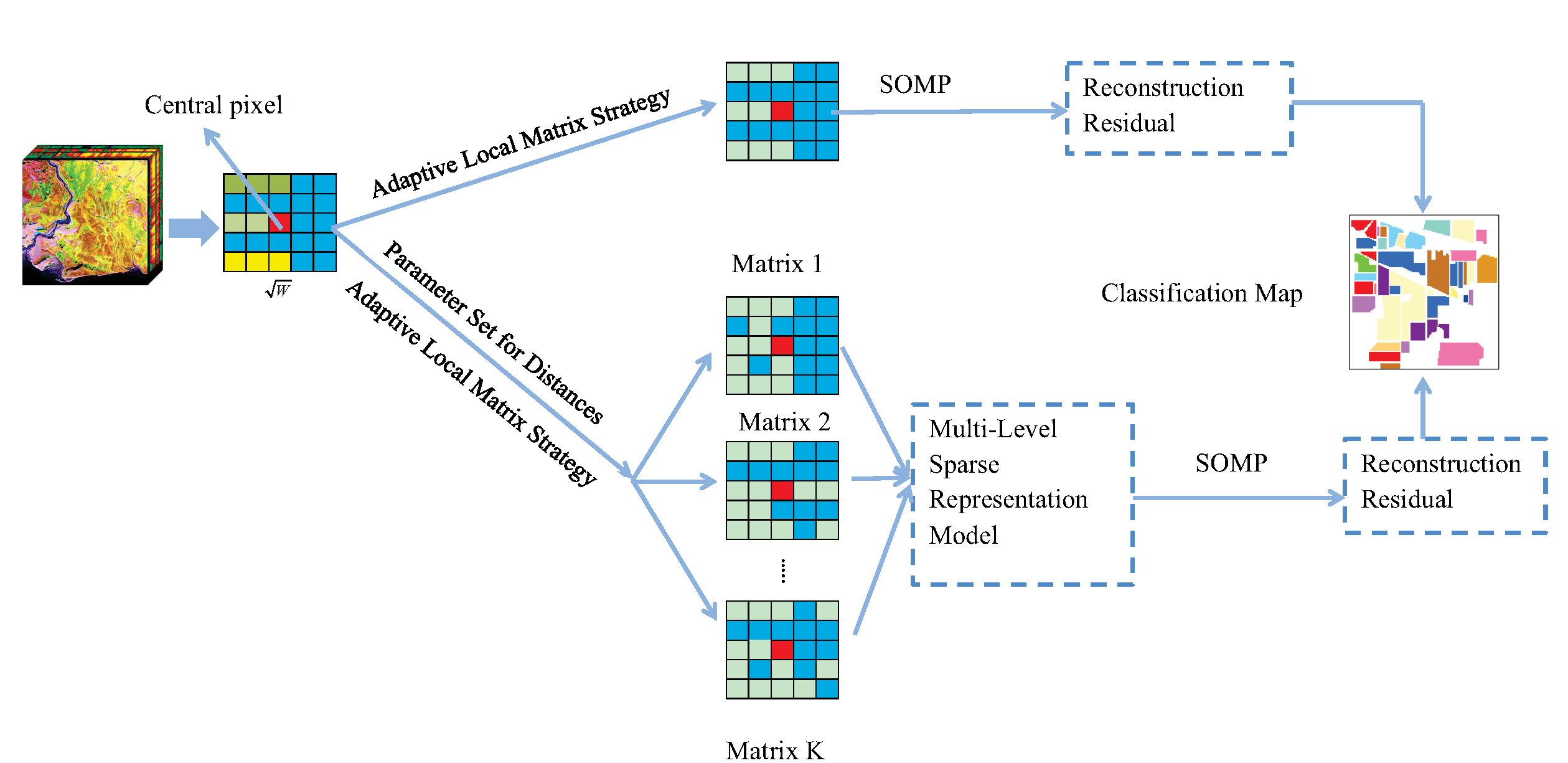
To better understand the procedure of the proposed method, a flowchart is shown in Figure 1 where each component of the method is explained in detail in the following sections.

3.1. Adaptive Local Signal Matrix

In order to select reasonable neighbours to construct the joint matrix, the weighted Euclidean distances between the test pixel and its neighbours are used. We first select a region with a window size $\sqrt{W}\times \sqrt{W}$, which is centred at the test pixel $x_i$. Different weights are given to each spectral band according to their contribution to the whole spectral characteristics. The weighting strategy is described as follows:

$$\begin{array}{l}A<x_i,x_j>=\sqrt{{\displaystyle \sum _{l=1}^L{w}_l{(x_{il}-x_{jl})}^2}}\\ w_l=\frac{\exp (\alpha I_l)}{{\displaystyle \sum _{l=1}^L\exp (\alpha I_l)}}\\ I_l=\frac{{\displaystyle \sum _{i=1}{\displaystyle \sum _{c}In(y_i=c){({\overline{x}}_{cl}-{\overline{x}}_l)}^2}}}{{\displaystyle \sum _{i=1}{\displaystyle \sum _{c}In(y_i=c){(x_{il}-{\overline{x}}_{cl})}^2}}}\end{array}$$

(12)

where $A<x_i,x_j>$ is the weight distance between pixels $x_i$ and $x_j$, $w_l$ is the weight for the l-th feature, and $w_l$ is determined by training samples from different classes. $\alpha$ is a positive parameter that controls the influence of a class-specific distance $I_l$. If $\alpha =0$, the distance between two pixels decreases to the equal weight Euclidean distance. If $\alpha$ is large enough, the change will be reflected on $I$. $In(\cdot )$ denotes an indicator function which takes between-class and within-class distances into account. ${\overline{x}}_{cl}$ is the average of the c-th class of the l-th feature, and ${\overline{x}}_l$ represents the average of all training samples of the l-th feature; $y_i$ represents the label of pixel $x_i$.

Pixels with a predefined distance value can be selected as similar neighbours according to this method. In other words, this adaptive neighbour selection strategy can identify the samples with similar characteristics to form a group. The superiority of this weight strategy over other weighting schemes is that it considers the spectral similarities on a pixel level, and the discriminative information among different groups which can be obtained from training samples.

3.2. Adaptive Weight Joint Sparse Model

The goal of Equation (12) is to find the optimal samples to reconstruct the central pixel. Once the appropriate weights are assigned to each spectral band, the weight distances between the test pixel and its neighbouring pixels can be evaluated. Based on the top N-nearest strategy, $N$ nearest neighbouring pixels can be chosen as the adaptive weight joint sparse matrix to relax the joint sparse model (Equation (9)). Here we define $S_N$ as the weight matrix chosen from the original joint sparse matrix $X=[x_1,x_2\dots x_W]$. In other words, $N$ nearest pixels are selected from the $W$ pixels based on the previous adaptive weight scheme. The adaptive weight joint sparse model can be expressed as:

$$\begin{array}{l}\stackrel{⌢}{R}=\arg \min {\Vert S_N-DR\Vert }_F\\ {\begin{array}{ccc}subject& to& \Vert R\Vert \end{array}}_{row,0}\le P\end{array}$$

(13)

The label of central pixel can be identified by minimizing the class residual:

$$Class(x)=\underset{c=1,2\dots C}{\arg \min }{\Vert S_N-D_c{R}_c\Vert }_F$$

(14)

The procedure of AJSM is summarized below in Algorithm 1.

Algorithm 1. The implementation of AJSM

Input: training datasets belong to the c-th class: $X_c$, region scale: $W$, top number of nearest neighbours: $N$, test datasets $X_T$. Initialization: initialize dictionary $D$ with training samples, and normalize the columns of $D$ to have unit ${\ell }_2$ norm. 1. Compute the $w_l$ for each spectral band according to Equation (12); 2. For each test pixel in $x_i\in X_T$:  Construct the weight matrix $S_N$ according to Equation (12) and normalize the columns of $S_N$ to have a unit ${\ell }_2$ norm;  Calculate the sparse coefficient matrix $R$ and dictionary $D$ from Equation (13) using SOMP;  Determine the class label $y_t$ for each test pixel $x_i\in X_T$ by Equation (14). Output: 2-dimensional classification map.

It has been identified that neighbouring pixels consist of different types of materials in the heterogeneous areas in HSI. JSM cannot perform well on such areas due to its definition of neighbouring pixels, which tend to have similar labels. The proposed AJSM is expected to improve the classification accuracy in these areas by not taking all the neighbouring pixels to construct the joint sparse matrix.

3.3. Multi-Level Weighted Joint Sparse Model

The neighbour pixels selected from a fixed scale using single level criteria as seen in JSM and AJSM may not contain the complementary and accurate information, and the neighbour pixels selected from different criteria levels can help represent the data wholly. Herewith we propose a multi-level weighted joint sparse model to fully integrate the neighbour information, as well as to avoid the outliers dominating in the sparse coding. For a test pixel, its neighbour pixels are selected by the proposed adaptive neighbour selection strategy with different distance threshold level values. Then the multiple joint sparse matrices are constructed by the corresponding neighbour pixels with different distance threshold level values. The details of this method are described as follows.

Assume that $S_{i,k}$ is the k-th joint sparse matrix constructed for pixel $x_i$. Here we define $S_{i,k}$ using a weight matrix i.e., $S_{i,k}=[\varpi <x_i,x_{i,1}>x_{i,1},\varpi <x_i,x_{i,2}>x_{i,2},\dots ,\varpi <x_i,x_{i,j}>x_{i,j},\dots ,\varpi <x_i,x_{i,W}>x_{i,W}]$ where $\varpi <x_i,x_{i,j}>$ is a function that determines if pixel $x_{i,j}$ can be preserved to reconstruct $x_i$, $x_{i,j}$ is the j-th sample in the given region which is restricted by the scale $\sqrt{W}\times \sqrt{W}$. In (12), $A<x_i,x_{i,j}>$ is a monotonously increasing function of the weighted distances. Although there are many ways to define $\varpi <x_i,x_{i,j}>$, we define it as a piecewise constant to simplify the selection of different joint sparse matrices as follows:

$$\varpi <x_i,x_{i,j}>=\{\begin{array}{c}\begin{array}{cc}1,& A<x_i,x_{i,j}>\le \epsilon \end{array}\\ \begin{array}{cc}0,& A<x_i,x_{i,j}>>\epsilon \end{array}\end{array}$$

(15)

where $\epsilon$ is a threshold controlling the value of the corresponding element in $S_{i,k}$. According to (12) and (15), when a pixel in $S_{i,k}$ has the corresponding weighted distance with the test pixel $x_i$: $A<x_i,x_{i,j}>>\epsilon$ it will not be selected in the joint sparse model. Otherwise, if $A<x_i,x_{i,j}>\le \epsilon$, the corresponding term will be selected to reconstruct the test pixel. In other words, $S_{i,k}$ is constructed by the terms that have the weighted distances less than $\epsilon$ between itself and the test pixel $x_i$.

By using the proposed scheme, we can generate different patches with various values of $\epsilon$:

• $\epsilon =0$: This is an independent set. In this situation, only the central pixel itself is selected. This means that the joint sparse model becomes a pixel-wise sparse representation model.
• $\epsilon \ge 1$: Because $A<x_i,x_{i,j}>\le 1$ in this situation, all the neighbours of the test pixel in the given area are selected.
• $0<\epsilon <1$: The sparsity representation of $x_{i,j}$ is satisfied. A smaller number of pixels are selected for the reconstruction of $x_i$.

As described above, for each test pixel $x_i$, when different parameters of $\left\{{\epsilon }_1,\dots ,{\epsilon }_k,\dots ,{\epsilon }_K\right\}$ are applied, $K$ different patches can be generated to represent this pixel with the inner contextual information involved. Our next task is to construct the multi-level joint sparse representation model for the test pixel.

3.4. Multi-Level Joint Sparse Representation

The SRC has been successfully used for HSI classification, herein we extend it to a multi-level version for the classification task. After $K$ different patches are constructed for each pixel, the patches for the test pixel can be arranged as a feature matrix: $S_i=[S_{i,1},\dots ,S_{i,k},\dots ,S_{i,K}]$($k=1,2,\dots ,K$), where $S_{i,k}$ be the k-th joint sparsity matrix constructed for the test pixel $x_i$.

In this paper, let $D=\{D^1,\dots ,D^k,\dots D^K\}$ be a set of dictionary which can be learnt from all the training data for $K$ patches, and $D^k$ is the dictionary learnt for the k-th level. Each dictionary $D^k$ is composed of all the sub-dictionaries for each labelled class as $D^k=[D_1^k,\dots ,D_c^k,\dots ,D_C^k]$, where $D_c^k$ denotes the sub-dictionary of the c-th labelled class.

The sparse representation of the test pixel $x_i$ with its k-th patch can be described as:

$$\underset{Q^k}{\min }{\Vert S_{i,k}-D^k{Q}^k\Vert }_F$$

(16)

where $Q^k$ is the sparse representation coefficients for the specific patch $S_{i,k}$. Equation (16) expresses how to sparsely represent each of the $K$ patches when the sparse coefficient vector is given. Considering all the $K$ patches, Equation (16) can be rewritten as:

$$\underset{Q}{\min }{\displaystyle \sum _{k=1}^K\left({\Vert S_{i,k}-D^k{Q}^k\Vert }_F\right)}$$

(17)

where $Q=[Q^1,\dots ,Q^k,\dots Q^K]$ is composed of $K$ columns of the coefficient vectors. Each column of the matrix is the sparse representation coefficients corresponding to a dictionary over a specific patch.

Since the pixels belonging to the same class should have the dictionary in the same subspace spanned by the training samples, the class-specific level joint representation optimization problem can be written as:

$$\langle \widehat{D},\widehat{Q}\rangle =\underset{D,Q}{\arg \min }{\displaystyle \sum _{k=1}^K\left({\Vert S_{i,k}-D^k{Q}^k\Vert }_F\right)}$$

(18)

This problem can be decomposed into $K$ sub-problems. In this paper, the SOMP is used to solve the optimization function (Equation (18)) and it can efficiently solve this problem in several iterations. Algorithm 2 introduces the implementation of the proposed framework.

After the sparsity coefficients are obtained, for a given test pixel $x_i$, it would be assigned to the class which gives the smallest reconstruction residual:

$$y_i=\underset{c\in 1,2,\dots ,C}{\arg \min }{E}_c(x_i)$$

(19)

where $E_c(x_i)$ is the reconstruction residual of $x_i$, as:

$$E_c(x_i)={\displaystyle \sum _{k=1}^K{\Vert S_{i,k}-D_c^k{Q}_c^k\Vert }_2^2}$$

(20)

where $D_c^k$ is the dictionary for the c-th class over the k-th patch, and $Q_c^k$ denotes the sparse coefficient matrix corresponding to $D_c^k$.

Algorithm 2. The implementation of the proposed algorithm.

Input: training datasets belonging to the c-th class: $X_c$, region scale: $W$, number of levels: $K$, distance threshold controlling parameter: $\epsilon$, test datasets $X_T$ Initialization: initialize dictionary $D_c=X_c$, and normalize the columns of dictionary to have unit ${\ell }_2$ 1. Compute $w_l(l=1,2,\dots ,L)$ according to Equation (12) using the training data sets $X_c$ and the corresponding labels 2. For each test pixel $x_i\in X_T$  Compute adaptive weight distances between the test pixel and all the pixels in the selected neighbour region to construct $A<x_i,x_j>$ based on Equation (12) 3. Compute $S_{i,k}$ based on Equation (15). 4. For $k=1:K$  Compute $Q^k$ for each level for each class using SOMP. 5. Compute the class label $y_i$ for test pixel based on Equations (19) and (20). Output: 2-dimensional classification map.

4. Experimental Results and Analysis

4.1. Data Description

To validate the proposed methods, three benchmark datasets are used in the experiments.

1. Airborne Visible/Infrared Imaging Spectrometer (AVIRIS) dataset: Indian Pines, which was obtained by an AVIRIS sensor over the site in Northwest Indiana, United States of America (USA). This imagery has 16 labelled classes. The dataset has 220 spectral bands ranging from 0.2 to 2.4 $\mathsf{\mu }\mathrm{m}$ wavelength, and each channel has 145$\times$145 pixels with a spatial resolution of 20 m. Twenty water absorption bands (no. 104–108, 150–163, and 220) are removed in the experiments. This data is widely used due to the presence of mixed pixels in available classes and the unbalanced number of training samples per class.

2. Reflective Optics System Imaging Spectrometer (ROSIS) data set: University of Pavia, Italy. This image was acquired during a fight campaign over Pavia in Northern Italy. It has nine labelled ground truth classes with 610$\times$340 pixels. This dataset contains urban features, as well as vegetation and soil features. Each pixel has a 1.3 m spatial resolution. With water absorption bands removed, 103 bands are used in the experiments.

3. AVIRIS data set: Salinas. The image was also acquired by an AVIRIS sensor over Salinas Valley, CA, USA. The image is of 512$\times$217 size with 224 spectral bands. In the experiments, 20 water absorption bands (no. 108–112, 154–167, and 224) are removed. Salinas has a 3.7 m resolution per pixel and 16 different classes. It includes vegetables, bare soils, and vineyard fields. Due to the spectral similarity of most classes, this dataset has been frequently used as a benchmark for HSI classification.

The ground truths of three datasets, as well as the false colour composite images are illustrated in Figure 2.

4.2. Description of Comparative Classifiers and Parameters Setting

In this paper, the proposed AJSM and MLSR are compared with several benchmark classifiers: pixel-wise SVM (referred to as SVM), EMP with SVM (referred to as EMP), pixel-wise SRC (referred to as SRC), and JSM with a greedy pursuit algorithm [28]. Pixel-wise SVM and pixel-wise SRC classify the images with only spectral information, while JSM, AJSM, and MLSR are sparse representation-based classifiers with spatial information utilized.

During the experiments, the range of parameters is empirically determined and the optimal values are determined by cross-validation. The parameters for pixel-wise SVM are set as the default ones in [4] and implemented using the SVM library with Gaussian kernels [41]. Parameters for EMP and pixel-wise SRC are set up by following the instructions in [14] and [28], respectively. The selected regions for JSM, AJSM, and MLSR are set as 3$\times$3, 5$\times$5, 7$\times$7, 9$\times$9, 11$\times$11, 13$\times$13 and 15$\times$15, and the best result is described in this paper. For AJSM, the number of pixels selected in the given region is set as: 7, 20, 40, 50, 50, 50, and 50 for the abovementioned scales, respectively. For the proposed MLSR, the number of threshold parameter $\epsilon$ is set as seven, and the threshold values are: $\left\{0.1,0.2,0.3,0.4,0.5,0.7,1\right\}$. The predefined sparsity level is set as 3 for each dataset.

Quantitative analysis metrics, overall accuracy (OA), average accuracy (AA), and Kappa coefficient are adopted to validate the proposed method. All the experiments in this paper are repeatedly implemented ten times and the mean accuracy is presented.

4.3. Experimental Results

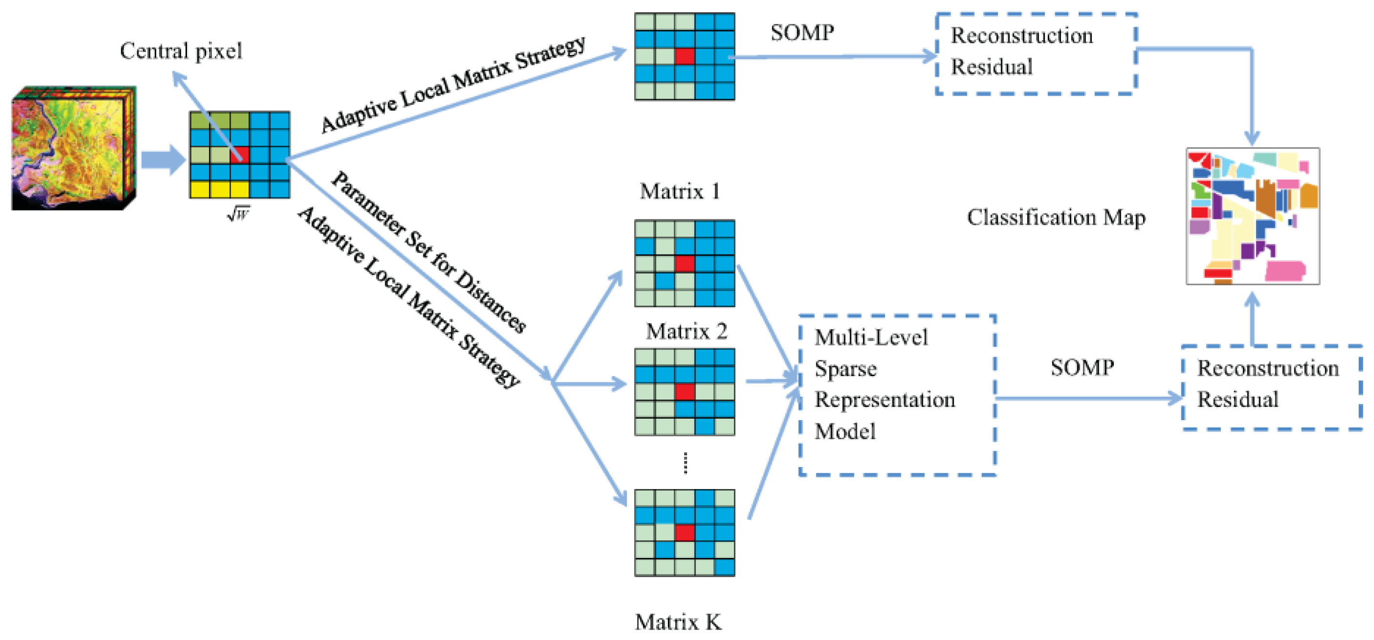
The first experiment was performed on the Indian Pines image. We randomly selected 10% of the samples from each class as training data and the remaining as a test dataset. The optimal parameters in this experiment are set as: $\alpha$= 0.2, $W=13\times 13$. The numbers of training and test data for each class are described in

Table 1. Class information for the Indian Pines dataset.

Class	Class Name	Training	Test
1	Alfalfa	5	41
2	Corn-no till	143	1285
3	Corn-min till	83	747
4	Corn	24	213
5	Grass/trees	49	434
6	Grass/pasture	73	657
7	Grass/pasture-mowed	3	25
8	Hay-windrowed	48	430
9	Oats	2	18
10	Soybeans-no till	97	875
11	Soybeans-min till	246	2209
12	Soybeans-clean till	60	533
13	Wheat	21	184
14	Woods	127	1138
15	Buildings-grass-trees	39	347
16	Stone-steel towers	9	84
Total		1029	9220

. Classification results are listed in

Table 2. Classification accuracies (%) for the Indian Pines image. The best results are shown in boldface.

Class	SVM	EMP	SRC	JSM	AJSM	MLSR
1	42.40	70.49	32.48	74.07	84.09	92.60
2	75.06	91.55	73.31	94.97	92.16	94.63
3	59.91	85.63	58.12	91.82	95.16	99.88
4	50.98	79.49	47.53	87.15	93.67	96.15
5	86.97	95.83	82.04	96.63	96.67	93.36
6	93.84	98.19	89.33	98.88	98.63	97.99
7	89.66	96.30	39.68	94.15	99.98	100.00
8	99.57	100.00	93.22	99.79	99.16	99.80
9	66.67	92.86	32.73	78.57	50.00	82.00
10	62.49	85.96	60.96	91.16	93.30	97.83
11	83.31	94.39	82.61	95.61	92.71	97.41
12	72.17	88.96	70.00	92.05	95.43	91.37
13	90.04	98.07	78.74	99.50	96.10	99.53
14	96.93	98.77	94.83	99.03	97.78	100.00
15	52.82	83.57	49.90	89.88	95.84	98.95
16	82.61	90.82	60.40	94.57	98.91	90.53
OA	75.41	90.77	65.82	92.52	94.74	97.08
AA	75.34	90.68	65.37	92.73	92.48	95.75
Kappa	73.71	91.20	69.90	94.25	94.02	96.79

, and the classification maps are shown in Figure 3. One can observe that the classification maps obtained by pixel-wise SVM and pixel-wise SRC have a more noisy appearance than other classifiers, which confirms that the contextual information is important for hyperspectral image classification. Considering the spatial information, JSM gives a smoother result; however, it still fails to classify some near-edge areas. EMP, AJSM, and the proposed MLSR deliver better results, and MLSR shows the highest classification accuracy. From Figure 3, one can see that MLSR further provides a smoother classification result and preserves more useful information for HSI.

The proposed AJSM improves the classification capability of JSM by exploring the different contributions of the neighbouring pixels in the selected region. This confirms the effectiveness of the adaptive weight matrix scheme. However, one can see that AJSM produces a relatively lower accuracy for oats, which has limited training samples. The improvement of MLSR-based classification of alfalfa and oats, which have been considered as small classes, indicates that the proposed method can perform well on classes with fewer training samples. In addition, the adaptive local matrix imposes the local constraint on the sparsity, which would improve the performance. As can be observed from the classification maps, our proposed method has a better capability to identify the near-edge areas and it benefits from the selection of most similar pixels to reconstruct the test pixel. The accuracies for MLSR are very high, which indicates that JSM can be significantly improved by multiple feature extraction approaches.

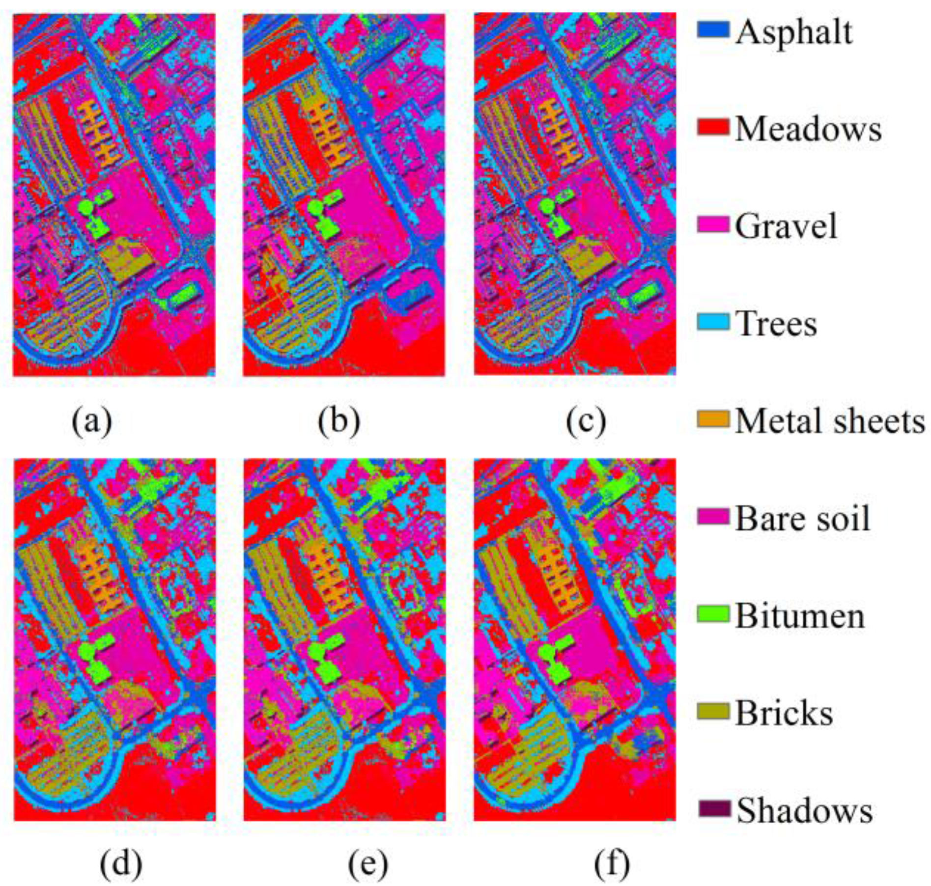
The second experiment is conducted on the Pavia University image, and

Table 3. Class information for the University of Pavia image.

Class No.	Class Name	Training	Test
1	Asphalt	250	6381
2	Meadows	250	18,399
3	Gravel	250	1849
4	Trees	250	2814
5	Meta sheets	250	1095
6	Bare soil	250	4779
7	Bitumen	250	1080
8	Bricks	250	3432
9	Shadows	250	697
Total		2250	40,526

shows the class information. We randomly selected 250 samples as the training data, and the rest as test data. The optimal parameters in this experiment are set as: $\alpha$= 0.2, $W=15\times 15$. Classification results and maps are illustrated in

Table 4. Classification accuracies (%) for the University of Pavia image. The best results are shown in boldface.

Class	SVM	EMP	SRC	JSM	AJSM	MLSR
1	77.42	84.38	73.46	86.84	99.41	96.32
2	96.34	97.81	95.35	98.07	92.59	99.38
3	84.03	91.44	79.53	91.47	87.09	99.90
4	72.41	81.58	68.07	83.23	98.50	97.68
5	99.92	99.93	99.92	99.11	99.11	100.00
6	82.67	88.81	78.52	90.19	90.16	100.00
7	95.07	96.65	93.64	97.27	95.19	99.92
8	92.39	95.97	89.74	96.46	84.87	99.65
9	99.89	99.54	97.65	86.54	100.00	95.04
OA	88.90	92.90	86.21	92.13	93.30	98.85
AA	88.92	92.95	86.47	93.73	94.10	98.65
Kappa	84.38	90.22	80.76	91.51	91.21	98.47

and Figure 4, respectively. It is obvious that the multi-level information can, indeed, improve the results of classification of the Pavia University image compared to other SRC based methods and the popular SVMs. The improvement of MLSR compared to JSM suggests that the local adaptive matrix can preserve the most useful information and reduce the redundant information. The result is consistent with the previous experiment on the Indian Pines image where the edge pixels are predicted more precisely.

The third experiment is conducted on the Salinas imagery. For each class, 1.5% samples are selected as the training data, and the remaining as the test dataset. The optimal parameters in this experiment are set as: $\alpha$= 0.2, $W=15\times 15$. The class information and classification results are given in

Table 5. Class Information for the Salinas image.

Class No.	Class Name	Training	Test
1	Weeds_1	30	1979
2	Weeds_2	56	3670
3	Fallow	30	1946
4	Fallow plow	21	1373
5	Fallow smooth	40	2638
6	Stubble	60	3899
7	Celery	54	3525
8	Grapes	169	11,102
9	Soil	93	6110
10	Corn	49	3229
11	Lettuce 4 week	16	1052
12	Lettuce 5 week	29	1898
13	Lettuce 6 week	14	902
14	Lettuce 7 week	16	1054
15	Vineyard untrained	110	7158
16	Vineyard trellis	27	1780
Total		814	53,315

and

Table 6. Classification accuracies (%) for the Salinas image. The best results are shown in boldface.

Class	SVM	EMP	SRC	JSM	AJSM	MLSR
1	98.62	99.50	98.67	99.31	99.75	97.83
2	99.65	99.76	99.65	99.70	99.58	97.97
3	95.44	97.95	95.63	97.02	98.73	100.00
4	97.25	98.43	97.39	97.94	98.92	98.85
5	97.73	98.30	97.76	98.18	98.62	99.51
6	100.00	99.90	100.00	99.92	99.77	99.92
7	98.11	99.42	98.16	99.11	99.86	99.72
8	78.87	90.74	79.91	86.79	80.18	89.77
9	99.56	99.77	99.61	99.76	98.90	99.48
10	90.60	96.03	91.13	94.12	93.72	98.96
11	89.01	95.75	89.79	93.07	99.44	100.00
12	96.05	98.45	96.40	97.55	99.07	100.00
13	94.77	96.67	94.87	95.62	97.60	99.13
14	87.11	94.25	87.56	91.44	96.17	98.13
15	59.09	79.50	60.62	71.87	82.44	97.41
16	98.28	99.17	98.39	99.16	98.78	98.56
OA	87.64	94.31	88.20	91.98	92.58	97.25
AA	92.51	96.47	92.85	95.04	96.33	98.77
Kappa	86.29	93.68	86.91	91.09	92.00	96.94

, respectively. The results are also visualized in classification maps as shown in Figure 5. One can observe that the proposed MLSR yields the best accuracy for most of the classes, especially for classes 15 and 16. Furthermore, the proposed MLSR identified the edge areas best.

4.4. Effects of Different Kinds of Parameters

This section focuses on the effects of the parameters setting on the classification performance. We first varied the value of positive parameter $\alpha$ that controls the influence of the ratio of the between-class and within-class distances, and the value was varied from 0 to 1 at 0.2 intervals. The experiments were conducted with AJSM on three datasets and the window sizes were fixed as the corresponding optimal values. In Figure 6, the overall accuracies for three datasets fluctuate in a small range, and the best performances were obtained when $\alpha$ was set as 0.2 for all three datasets though the trends for them were different. As $\alpha$ only controls the influence of each feature band, it is reasonable to apply the same value for MLSR in the experiments.

The effect of region scales for JSM, AJSM, and MLSR has also been analysed in the experiments. In order to simply show the trends, the numbers of training and test datasets are selected to be the same as in the previous experiments. OA is shown in Figure 7. For JSM, AJSM, and MLSR, the region scales ranging from 3$\times$3 to 29$\times$29 at 2$\times$2 intervals. As shown in Figure 7, the best OA is achieved for JSM when the scale is set as 7$\times$7, 11$\times$11, and 15$\times$15 for Indian Pines, Pavia University, and Salinas, respectively. If the scale increases, the accuracy decreases dramatically. In most situations, AJSM performs better than JSM because the most useful information is preserved and the redundant information is rejected by the selection strategy. The accuracy for MLSR becomes stable when a larger region is selected. More specifically, the proposed MLSR performs better than other joint sparsity-based models in most regions. This result actually benefits from its mechanism of discarding outliers in the specific area, which provides a more reliable dictionary.

Another consideration is the number of patches that should be tested, i.e., is having more patches better? To evaluate this, the adaptive framework is used to generate more patches. Especially, with $\epsilon$ set to $\left\{0.1, 0.2, 0.3, 0.4, 0.5, 0.6, 0.7, 0.8, 0.9, 1\right\}$, we can define 11 patches. In each experiment, we randomly selected a patch subset with the number of $K\in \left\{1,2,3,4,5,6,7,8,9,10,11\right\}$ from these 11 patches and evaluated the performance of the method on three datasets. For each value of $K$, the experiment procedure is repeated 10 times with different subset selection. Figure 8 shows the average OA result of the 10 iterations. As $K$ increases, the performance of the framework also increases when $K\le 7$; however, it slightly decreases when $K\ge 8$. This trend shows that a certain number of patches are necessary for the improvement of the performance of the proposed method. However, too many patches can also result in a slight decrease in performance. In the experiment, we fixed five values {0.1, 0.2, 0.3, 0.4, 0.5}, and the last two values are determined from the remaining five values {0.6, 0.7, 0.8, 0.9, 1} by cross-validation.

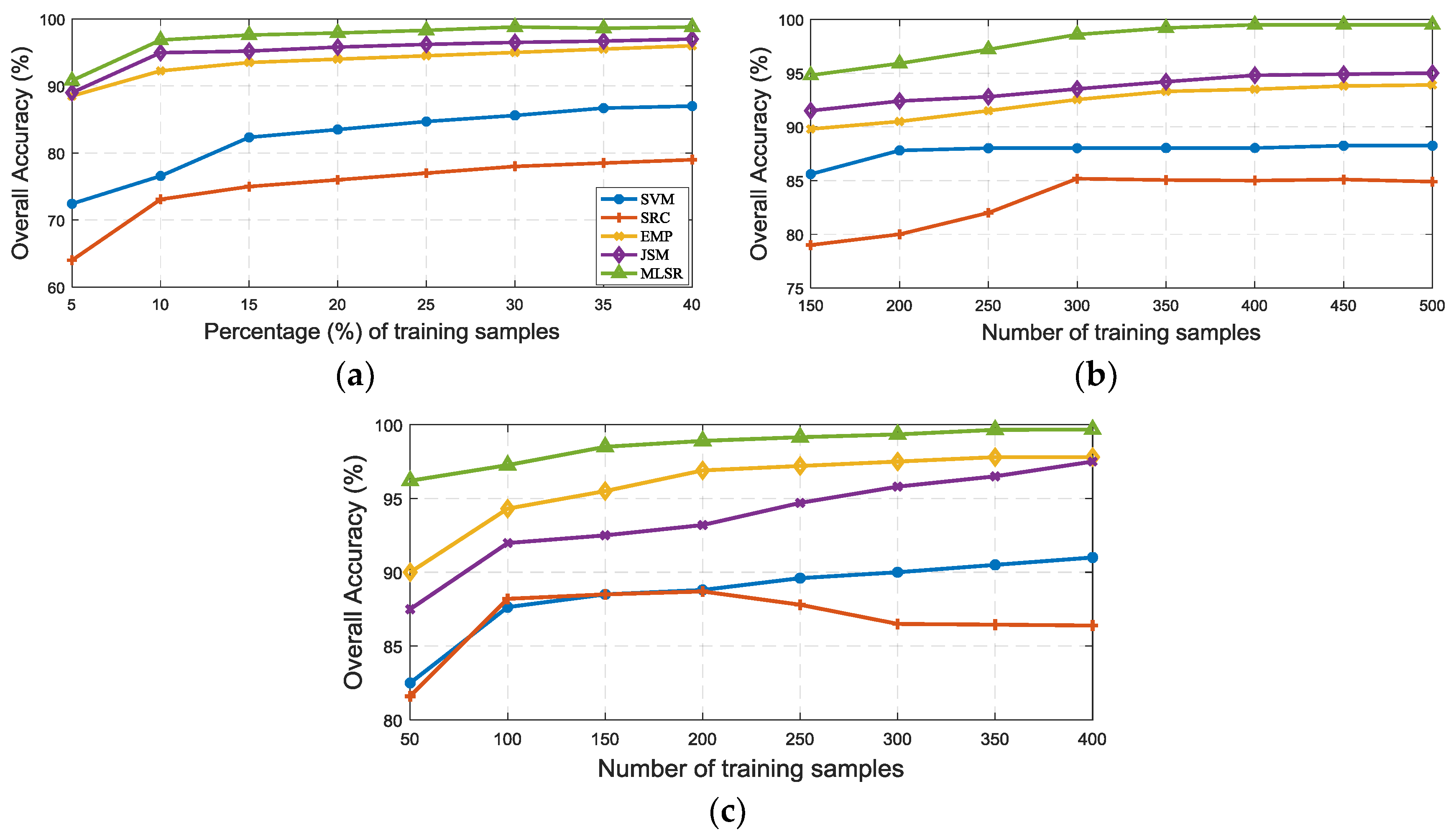
We also conducted the experiments to evaluate the impact of the number of training samples per class for pixel-wise SVM, pixel-wise SRC, EMP with SVM, single-scale JSM, and the proposed MLSR. AJSM is not considered in this experiment as they exhibit a similar trend with JSM. Training samples are randomly chosen, and the rest are used as test samples. For the Indian Pines dataset, the number of training data ranges from 5% to 40% of the whole pixel counts at 5% intervals; for the Pavia University dataset, the number of training samples per class ranges from 150 to 500 at 50 intervals; For the Salinas dataset, the number of training samples per class ranges from 50 to 400 at 50 intervals. Figure 9 illustrates the classification results (OA) for these three datasets. As can be observed, less than 5% of the samples are needed for each class to obtain an OA over 90% for the Indian Pines datasets using the proposed MLSR. This is very promising because it is often difficult to collect a large training datasets in practice. For the Pavia University dataset, only 150 training samples are needed to obtain an OA of 95%. In fact, this accuracy is 3% higher than that by JSM and 4.5% higher than that by EMP with SVM. This is due to the fact that the local information included by the proposed MLSR outperforms the others. The same trend can be concluded for the Salinas dataset. In addition, the proposed MLSR produces very high accuracy and shows robustness with an increase of the number of training samples, and it can be observed that MLSR performs very well when training samples are limited.

5. Conclusions and Future Research Lines

In this paper, we have introduced two novel sparse representation-based hyperspectral classification methods. These proposed methods employ an adaptive weight matrix scheme as the neighbour selection strategy for the joint sparse matrix construction. The adaptive weight joint sparse model outperforms the traditional joint sparse models, however, it is designed for simple cases rather than complicated situations where the number of labelled training samples is not sufficient. This was overcome by introducing the second model, i.e., the multi-level joint sparse model that can solve the complex classification problem in a more effective way. The multi-level joint sparse model consists of two main parts: adaptive locality patches and a multi-level joint sparse representation model. This model is introduced to fully explore the spatial context within a given region for the test pixel. The proposed methods locally smooth the classification maps and preserve the relevant information for most labelled classes. Compared with other spatial-spectral methods and sparse representation-based approaches, the proposed methods can provide a better performance on real hyperspectral scenes. This is consistent with the observation from the classification maps. Moreover, the experiments on the impact of the number of training samples also indicate that the proposed multi-level sparse approach leads to a more reliable result when only a limited number of training samples are available.