High Temporal Resolution Refractivity Retrieval from Radar Phase Measurements


Signal Theory and Communications Department, University of Vigo, 36310 Vigo, Spain
*
Author to whom correspondence should be addressed.
†
These authors contributed equally to this work.
Remote Sens. 2018, 10(6), 896; https://doi.org/10.3390/rs10060896
Submission received: 14 March 2018
/
Revised: 4 June 2018
/
Accepted: 5 June 2018
/
Published: 7 June 2018
(This article belongs to the Special Issue Remote Sensing of Land-Atmosphere Interactions)
Abstract
:Knowledge of the spatial and temporal variability of near-surface water vapor is of great importance to successfully model reliable radio communications systems and forecast atmospheric phenomena such as convective initiation and boundary layer processes. However, most current methods to measure atmospheric moisture variations hardly provide the temporal and spatial resolutions required for detection of such atmospheric processes. Recently, considering the high correlation between refractivity variations and water vapor pressure variations at warm temperatures, and the good temporal and spatial resolution that weather radars provide, the measurement of the refractivity with radar became of interest. Firstly, it was proposed to estimate refractivity variations from radar phase measurements of ground-based stationary targets returns. For that, it was considered that the backscattering from ground targets is stationary and the vertical gradient of the refractivity could be neglected. Initial experiments showed good results over flat terrain when the radar and target heights are similar. However, the need to consider the non-zero vertical gradient of the refractivity over hilly terrain is clear. Up to date, the methods proposed consider previous estimation of the refractivity gradient in order to correct the measured phases before the refractivity estimation. In this paper, joint estimation of the refractivity variations at the radar height and the refractivity vertical gradient variations using scan-to-scan phase measurement variations is proposed. To reduce the noisiness of the estimates, a least squares method is used. Importantly, to apply this algorithm, it is not necessary to modify the radar scanning mode. For the purpose of this study, radar data obtained during the Refractivity Experiment for HO Research and Collaborative Operational Technology Transfer (REFRACTT_2006), held in northeastern Colorado (USA), are used. The refractivity estimates obtained show a good performance of the algorithm proposed compared to the refractivity derived from two automatic weather stations located close to the radar, demonstrating the possibility of radar based refractivity estimation in hilly terrain and non-homogeneous atmosphere with high spatial resolution.
1. Introduction
Knowledge of the spatial and temporal variability of near-surface water vapor is of great importance to forecast convective initiation and boundary layer atmospheric processes [1]. In fact, the results in [2] indicate that the development of drylines is related to the initiation of deep moist convection. In addition, it has been shown that small variations in temperature (≈1 C) and moisture (≈1 g·kg) can make the difference between the initiation or not of a convective process [3,4]. Furthermore, it has also been reported that a spatial resolution, on the order of 2–5 km, is desired to define an accurate retrieval algorithm [5]. However, the lack of an adequate method to observe moisture variations with such accuracy and spatial resolution is one of the main limitations for the development of accurate numerical weather prediction methods [6]. Radar measurements of refractivity may help to improve the temporal resolution of water vapor pressure data over small areas since, at warm temperatures, the atmospheric refractivity is a good proxy for water vapor pressure. For example, at 18 C, a change of 1 C in temperature or a much smaller change of 0.2 g·kg in water vapor results in refractivity changes of 1 N-unit. That is, refractivity variations are mainly linked to water vapor variations at warm temperatures [7,8].
Additionally, the knowledge of the near-surface atmospheric refraction variability with enough spatial and temporal resolution is also fundamental to successfully design reliable radio communications systems, since it is needed for the electromagnetic tools devoted to the analysis and prediction of wave propagation [9], e.g., the parabolic equation method [10,11], for forward one-way [12] and forward-backward two-way propagation models [13]. Further development of current communication systems require accurate electromagnetic coverage prediction tools that help in spectrum management and reuse, interference mitigation and cognitive radio applications [14].
Weather radars are mainly used to detect and follow precipitation. Nevertheless, at low scanning elevation angles, ground clutter can also be observed. Taking advantage of this, it was demonstrated that the atmospheric refractivity can be derived from radar phase measurements providing an accuracy and a resolution not attainable by any other measurement methods at this moment (radiosonde launches, GPS occultation techniques [15,16], ...) while maintaining the essential functionality of weather radars [17]. In particular, the method retrieves temporal changes of the mean atmospheric refractivity over small areas at the radar height from phase measurements of the waves backscattered from stationary ground-based targets, assuming propagation over flat terrain and a zero vertical gradient of the refractivity [18]. First results, obtained with the McGill S-Band coherent radar in the Montreal area, provided a temporal resolution of about 5 min over areas of about 4 × 4 km. However, it must be pointed out that the size of the area over which the mean atmospheric refractivity is calculated is strongly dependent on the density of the stationary ground-based targets around the radar [18]. Refractivity coverage up to a range of 50–60 km from the radar can be obtained under standard propagation conditions.
Since then, several international experiments have been conducted in order to provide near-surface high-resolution water vapor information. The International HO project (IHOP_2002), held in the Southern Great Plains in Oklahoma (USA), focused on four complementary research topics: quantitative precipitation forecasting, convection initiation, atmospheric boundary layer processes and instrumentation for improving the understanding and the prediction of convective processes [19]. Results from IHOP_2002 revealed a close agreement between radar refractivity retrieval and weather ground-based stations measurements [7].
The Refractivity Experiment for HO Research and Collaborative Operational Technology Transfer (REFRACTT), held in northeastern Colorado (USA), provided the opportunity to improve the understanding of water vapor gradients and the role they play in the initiation of convection and thunderstorms over a several hundred kilometer domain using the Multi Next Generation Weather Radar network (NEXRAD) [20].
In general, comparisons of atmospheric refractivity estimated from weather radar data and surface weather stations measurements showed a high agreement, both spatially and temporally [21,22]. Interestingly, boundary layer convergence zones were identified prior to their appearance in reflectivity or Doppler velocity fields [7].
The interest in radar refractivity retrieval has become global and other interesting experiments have been conducted in the United Kingdom [23] and France [24,25]. Moreover, the algorithms for refractivity estimation have been validated at different operating radar frequencies: S-Band [8], C-Band [26] and X-Band [27]; and using phased array radars [28]. Moreover, the measurement algorithms, originally designed for coherent klystron transmitters, have been successfully modified to be used with non-coherent magnetron transmitters [29,30,31].
To improve the results of the algorithms to estimate the atmospheric refractivity from weather radar measurements, different sources of error have been analyzed, e.g., vegetation sway by the wind [18], reference map representativeness [22], phase-correlated returns [32], uncertainty in target location inside the gate [23], phase ambiguities [33] or the frequency drift when a non-coherent transmitter is used [23,31]. To reduce the noisiness, spatially smoothing of the phase variation measurements by either a pyramidal weighting function over a 4 × 4 km base [18] or a least squares method [32] has been proposed.
However, the assumptions of the method -flat terrain and a zero vertical gradient of the refractivity- severely limit the areas where the method can be applied since the actual non-zero refractivity vertical gradient and the height difference between the radar and the targets can lead to a significant bias of the estimated refractivity. In order to expand the applicability of the method to non-flat areas with a non-zero refractivity vertical gradient, different approaches have been proposed. Estimating the vertical profile of the refractivity from radar clutter measurements has been addressed in a number of works [34,35,36]. A comprehensive review is done in [37]. The approach proposed is based on finding the vertical profile of the refractivity that minimizes some measure of the difference between the sea clutter response at the radar and the predicted clutter response for a vertical profile. This is a complex inverse problem. The accuracy of the scattering/propagation method considered for the clutter response prediction and the performance of the inversion algorithm required determine the overall behaviour of the approach. In [38,39], the refractivity over hilly terrain, considering a varying refractivity vertical gradient, is retrieved from previous estimation of the refractivity vertical gradient from the ground coverage reached by the radar. Unfortunately, the limited accuracy of radar coverage estimates is transferred to refractivity vertical gradient estimates. In [40], it was proposed to previously estimate the refractivity vertical gradient from power measurements at two elevation angles. The variation of the refractivity vertical gradient between the measurements at different elevation angles affects the accuracy of this method. In fact, comparisons of the results obtained for the refractivity with in situ measurements of the refractivity showed a significant bias and a large variance of the refractivity retrieved from radar measurements due to the limitations of the methods for estimating the refractivity vertical gradient. Nevertheless, the results obtained with the previous methods demonstrated the impact of a non-zero refractivity vertical gradient on refractivity estimates.
In this paper, an approach to jointly and simultaneously retrieve the atmospheric refractivity and its vertical gradient over small areas from radar phase measurements with high temporal resolution, without modifying the radar scanning mode, is proposed and discussed. This method does not require considering flat terrain. Regarding the refractivity vertical gradient, following ITU-R P.453-11 Recommendation, it is assumed that it decreases linearly with height [41]. Measurements obtained during the Refractivity Experiment for HO Research and Collaborative Operational Technology Transfer (REFRACTT) [20], held in northeastern Colorado (USA) have been used to prove and validate the method. In fact, refractivity retrievals obtained from radar phase measurements showed a good agreement with data from ground-based weather stations located inside the influence area of the radar.
The remaining sections are organized as follows. In Section 2, the study area as well as the available data sources are described. The theoretical background for the retrieval of refractivity from radar phase measurements is briefly outlined in Section 3. In Section 4, refractivity derived from radar phase measurements is compared with refractivity measurements derived from automatic weather stations. Results are discussed in Section 5. Finally, the main conclusions of this research are presented in Section 6.
2. Study Site and Data Sources
2.1. Study Area
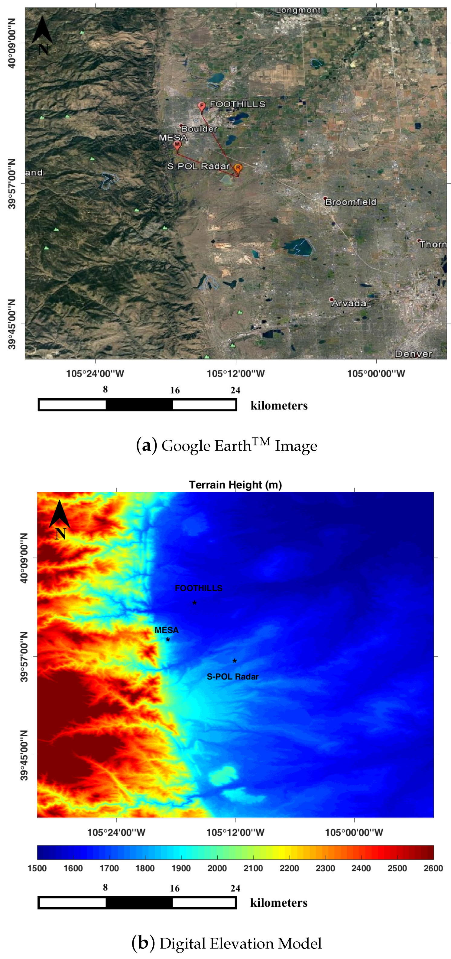
Data were collected during the Refractivity Experiment for HO Research and Collaborative Operational Technology Transfer () held at the base of the Foothills of the Rocky Mountains in Boulder (Northeast Colorado, USA) (Figure 1a). An elevation range of 1500 m to 2600 m above sea level is found inside the study area of 50 × 50 km centered in the radar location (3939′00 N to 4015′00 N, 10530′00 W to 10454′00 W) as shown in Figure 1b.
2.2. Data Sources
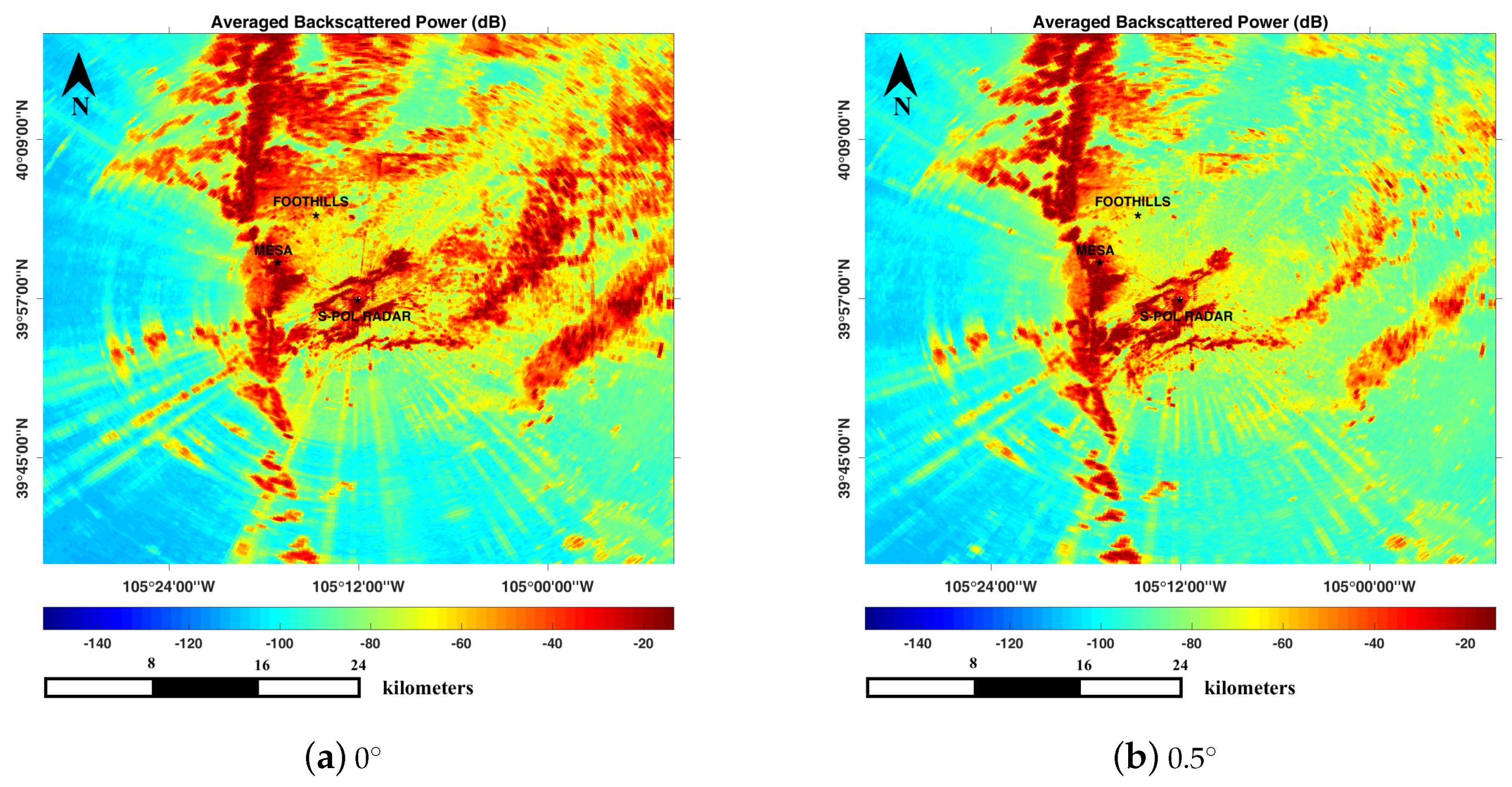
Radar measurements were collected using the S-Band Dual-Polarization Doppler Coherent Radar of the National Center for Atmospheric Research (NCAR S-Pol Radar) [42,43]. For this study, a total of 356 Plan Position Indicators (PPIs) collected from 12:00 a.m. UTC to 10:15 p.m. UTC on 1 August 2006 are considered. This amount of data results in a high temporal resolution of just over 3 min and a half. Scanning elevation angles of and were considered. Figure 2 shows the averaged backscattered power for both elevation angles along the full time interval. The radar technical specifications and the operational parameters are given in Table 1.
The digital elevation model (DEM) from the National Elevation Dataset of the U. S. Geological Survey (USGS) was used to derive the topography and to obtain the height of the targets. The height is sampled with an approximate spatial resolution of m in latitude and m in longitude. Figure 1b shows the topography of the study area. A height of 15 m above ground level is considered for the targets, since most of them are poles along the road, telecommunication towers or buildings. For the radar, considering the size of the antenna dish and of the supporting structure, a height above ground level of 15 m is assumed.
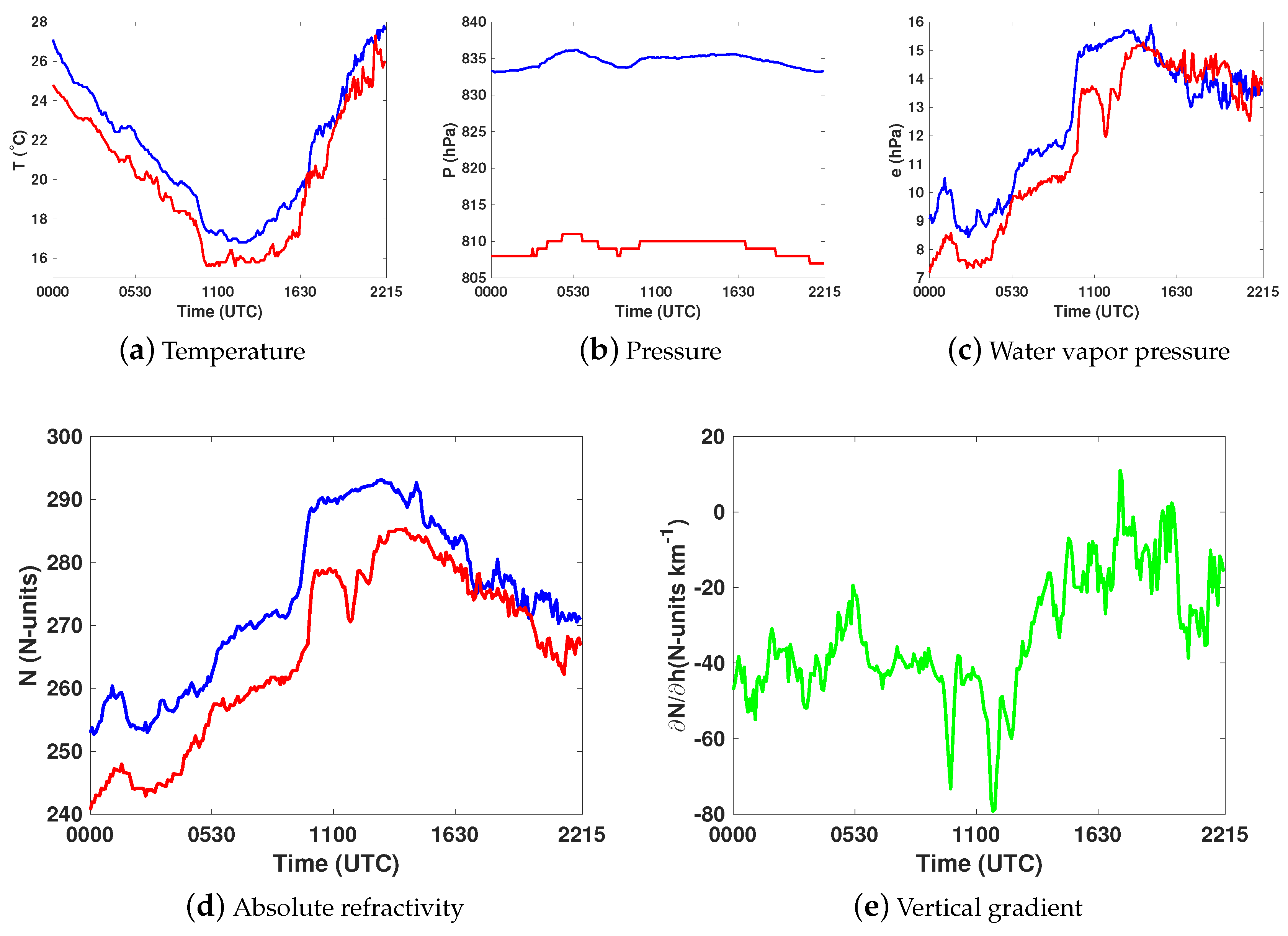
Two automatic weather stations, located at Foothills and Mesa (see Figure 1a,b), were used to derive in situ refractivity measurements. Automatic weather stations provided observations of atmospheric pressure (p[hPa]), temperature (T[K]) and water vapor pressure (e[hPa]) from which the refractivity was derived [44]:
A total of 267 joint observations of pressure, temperature and water vapor at 5 min time steps were collected while radar measurements were taken (from 12:00 a.m. UTC to 10:15 p.m UTC on 1 August 2006). Table 2 provides the location parameters of the automatic weather stations and their position with respect to the radar. Information about the radar and automatic weather stations data collected are summarized in Table 3.
3. High Temporal Resolution Estimation of Mean Refractivity and Refractivity Vertical Gradient over Small Areas
3.1. Radar Refractivity Algorithm
In the lower part of the atmosphere, where weather radars are operated, it can be assumed that the refractive index of the atmosphere linearly decreases with height [41]:
where is the refractive index of the atmosphere at the radar height , arc distance s and time t, and is the vertical gradient of the refractive index at time instant t, assumed to be constant with height and arc distance.
As a consequence of the variation of the refractive index with distance and height, the electromagnetic wave does not follow a straight path, but it bends as it propagates. Its phase will be determined by the actual path, C, followed by the wave and the refractive index along the path:
That is, considering that the height of the ray path along the range r is described by and the refractive index in the lower troposphere is as given in Equation (2), the phase of the wave travelling from the radar to a target at range and back is
where is the phase of the ground target scattering coefficient and the sub-index t in is used to stress that the range to the target varies with time.
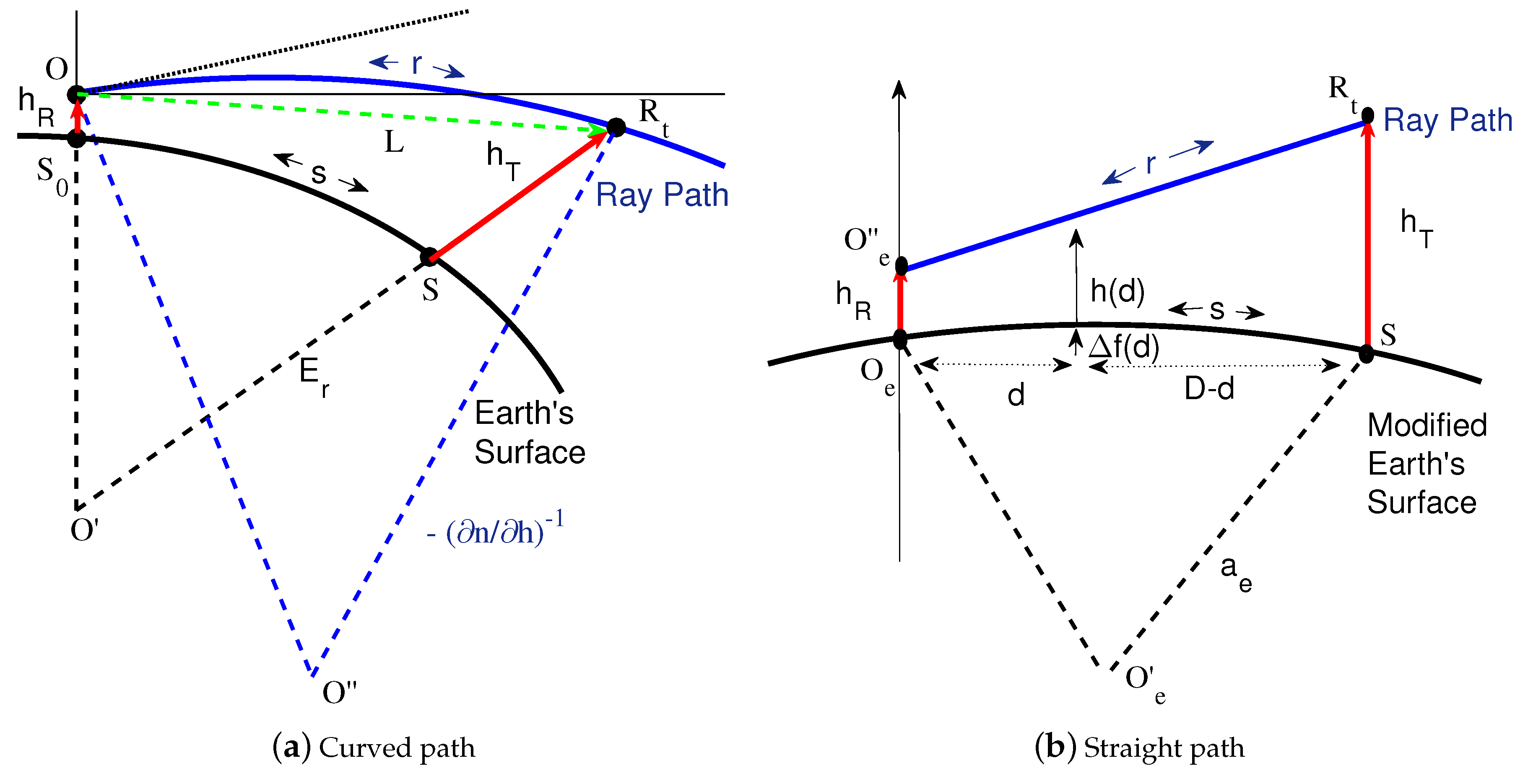
The range, , travelled by the ray, from the radar to the target , at time t is obtained (see Figure 3a) [38] assuming that, for low elevation angles, the ray curvature can be considered constant along the ray path, its radius can be approximated by and the arc distance S between the radar and the target at the Earth’s surface is known:
with
where is the height of the ground target above sea level and the Earth’s radius.
To evaluate the integral in Equation (4), the equivalent Earth model (see Figure 3b) is considered [45]. In this model, the Earth’s radius is modified so that, keeping the curvature difference between the Earth and the ray constant, the rays propagate in a straight line. Then, the height of the ray path to the target along the range r, , is given by [38]:
and, substituting Equation (7) into Equation (4), it is found that the phase of the wave backscattered from target is given by :
where is the radius of the equivalent Earth and is the mean refractive index along the arc path at height between the radar and the target :
Equation (8) shows the relationship between the backscattered wave phase at the radar and the refractive index. Changes in the refractive index result in phase variations. Unfortunately, the phase measured at the radar can only take on values within , i.e., the phase wraps every half wavelength increment of the path range preventing the estimation of the refractive index or its gradient from absolute phase measurements. Alternatively, it has been proposed to estimate refractive index variations from phase measurement variations between two time instants and and a pair of targets and [17]. Thus, the phase variation between a couple of targets and and two time instants and can be expressed as:
with
and
being the increment of the range to the target in the time interval , the increment of the mean value of the refractive index between targets and in the same time interval and the time variation of the refractive index vertical gradient between and . Additionally, it has been considered that the scattering coefficient phase of stationary ground clutter does not vary in time .
3.2. Joint Estimation of the Refractive Index and the Refractive Index Vertical Gradient Variations
The inversion of Equation (10) to retrieve the variations of the mean refractive index and of the refractive index vertical gradient is difficult. In order to obtain a simpler equation relating the phase variation between and and two consecutive time instants and with the variations of the mean refractive index and of the refractive index vertical gradient, the contribution of each term in Equation (10) to the phase variation has been analyzed (see Appendix A).
It was found that the contribution of some terms, namely , and , is negligible, so Equation (10) can be simplified to:
which shows a linear relation the phase variation between and from to with the variation of the mean refractive index between and at the radar height from to , , and the variation of the refractive index vertical gradient from to .
Let us consider that backscattering from N + 1 targets is available for a given area within which can be assumed constant. Then, the variation of the mean value of the refractive index is the same for all inter-targets paths along one azimuth direction, and up to N independent equations can be obtained and a least squares method can be used to estimate and :
The resolution in range will be defined by the maximum distance in range between any two targets, the resolution in azimuth by the maximum angular distance between any two targets and the temporal resolution will equal the time between scans. A higher resolution in range × azimuth can be achieved at the expense of increasing the variance of the estimates since some target pairs will not be inside the reduced resolution area.
In order to analyse the performance of the proposed method, the root mean square error (RMSE) and the bias (BIAS) between refractivity and refractivity vertical gradient variations derived from the radar and refractivity and refractivity vertical gradient variations derived from the weather stations are computed. The RMSE and BIAS for refractivity variations are defined as:
where is the variation of the refractivity derived from the radar from to and is the variation of the refractivity derived from the automatic weather stations measurements at the same time instants. For that, data derived from automatic weather stations are interpolated at the same time instants that radar data were taken. The same definition is used for refractivity vertical gradient variations changing by .
4. Results
4.1. Refractivity from Automatic Weather Stations
Observations of temperature, atmospheric pressure and relative humidity from two automatic weather stations (Foothills and Mesa) were used to derive the atmospheric refractivity. Figure 4a–c shows the meteorological observations at each station. The lower values of temperature and pressure at Mesa location are due to its higher altitude. Figure 4d shows the refractivity derived from the observations. As expected, it is generally higher at Foothills because of its lower altitude. Finally, Figure 4e shows the refractivity vertical gradient estimated from the difference in refractivity measurements at the Mesa and Foothills locations with a height difference of 260 m. It is worth noting that the assumptions considered previously in the analysis of the contributions to the total phase are consistent with the maximum variations of refractivity and vertical gradient derived, respectively, from Figure 4d–e considering 5 min time instants ( N-units and N-units ).
4.2. Stationarity Index of a Target
To estimate refractivity from radar phase measurements, the stationary targets must be identified. In this study, the stationarity of a target is determined considering the averaged backscattered power, its standard deviation and the reliability index (RI) defined in [28]:
where S is the number of scans considered (356 scans in our case) and the phase measured at the l-th PPI.
The index takes values between 1 (for completely stationary targets) and 0 (for completely random targets). Targets with a RI greater than 0.7, an averaged backscattered power higher than dB and a standard deviation of the averaged backscattered power lower than 2 dB are considered stationary targets.
4.3. Refractivity from Radar Phase Measurements
Spatial smoothing by a pyramidal weighting function over a 4 × 4 km base [18] has been commonly used to reduce the noisiness of the phase variation measurements over flat terrain. This smoothing acts as a band-pass filter centered on the average refractivity previously estimated over a certain area. As a result of this smoothing, faster fluctuations due mainly to phase noise are removed while slower fluctuations due to local variations of refractivity are retained.
Over hilly terrain, accurate estimation of the refractivity at the radar height requires simultaneous estimation of the refractivity vertical gradient. In this case, the fluctuations in the phase variations, due to the variability of the heights of the targets, can be quite fast; and therefore smoothing of the phase would lead to underestimate the vertical gradient variations. The refractivity estimates presented in here have been made from a careful selection of targets based on the RI, the averaged backscattered power and its standard deviation without smoothing the phase variation measurements.
Additionally, to reduce the probability of wrapping, which increases when height differences between the radar and the targets exist, consecutive PPIs are considered to obtain .
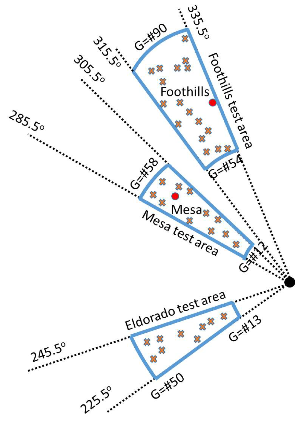
To analyze the performance of the least squares based algorithm proposed for the joint estimation of the mean refractivity variation and the vertical gradient refractivity variation, three different test areas, to the West of the NCAR S-Pol radar, of around 6 km in range by 20 in azimuth have been defined: the Foothills test area, the Mesa test area and the Eldorado test area, Figure 5. The Foothills and Mesa test areas have been defined around the Foothills and Mesa weather stations where already significant height differences between the targets and the radar are found. The Eldorado test area, though it does not contain any weather station presents higher height variations (the average altitude of the stationary targets within this area is 1810 m) and the results achieved here can be analyzed in comparison to the results obtained at Foothills and Mesa test areas.
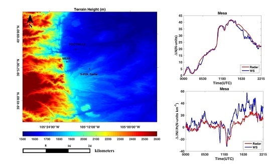
Figure 6a,b shows the mean refractivity variation at the radar height (in red) estimated from phase measurements from Mesa and Foothills test areas. It is compared with the refractivity variation at the radar height estimated from Mesa and Foothills weather stations data. Figure 6c,d shows the absolute mean refractivity derived from the estimates of the mean refractivity at the radar height and the vertical gradient of the refractivity (red line), and the absolute refractivity derived from weather station data (blue line) at the weather station heights. A good agreement is observed at radar height as well as at the weather stations heights between the refractivity derived from weather stations data and the refractivity derived from radar phase measurements. The RMSE and BIAS of the refractivity estimates shown in Figure 6a–d are summarized in Table 4.
The refractivity vertical gradient variation derived from the weather stations data (blue line) and the refractivity vertical gradient variation derived from radar phase measurements (red line) are shown in Figure 6e,f. The RMSE and BIAS of the refractivity vertical gradient estimates obtained for Mesa and Foothills test areas are also gathered in Table 4. Regarding the higher bias and variance observed for the refractivity vertical gradient estimates, it is of interest to point out that it is due to the higher noise caused by the height variations of the targets (that affect mainly the coefficients of the refractivity vertical gradient, see Equation (12). It is worth mentioning, though, that the correlation coefficient between the estimates of the refractivity vertical gradient variation independently derived for the Mesa and Foothills areas is very high, 0.831.
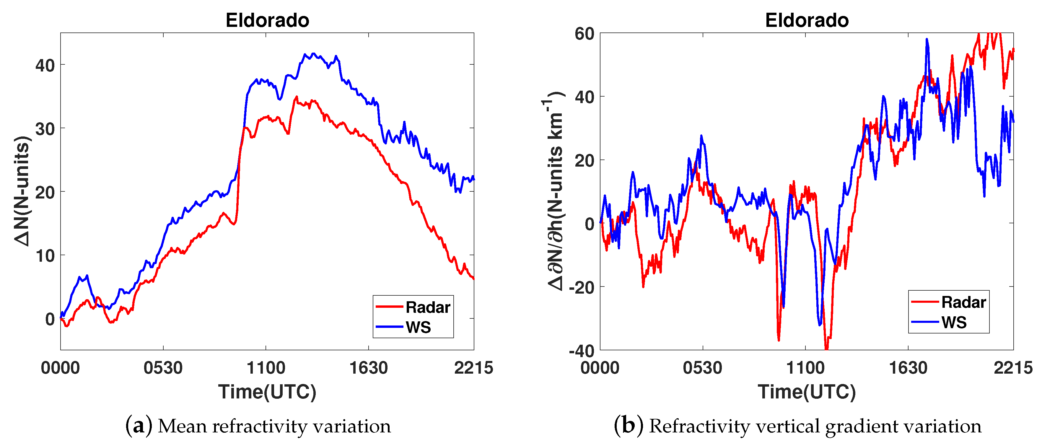
Figure 7a,b shows the mean refractivity variations at the radar height and the refractivity vertical gradient obtained from radar phase measurements of the Eldorado test area. In Figure 7a, the mean refractivity variation at the radar height estimated from Foothills and Mesa weather stations data is shown just for reference to observe the general agreement in the behavior of both estimates of the mean refractivity variation, from radar measurements and from weather station measurements. The higher discrepancies, as compared to Figure 6a,b are expected as there is a significant distance between Mesa-Foothills test areas and Eldorado test area. On the other hand, very high correlation coefficients of 0.809 (between the refractivity vertical gradient variation independently estimated at Mesa and Eldorado) and 0.776 (at Foothills and Eldorado) are obtained.
5. Discussion
The results obtained show the possibility and potential of the joint estimation of the refractivity vertical gradient and the mean refractivity at the radar height in hilly terrain. This last remark is important since, to estimate the refractivity vertical gradient, it is required to have targets at different heights. If there is not a significant height difference between the radar and the targets (on the order of 100 m or more), the system in Equation (12) becomes ill-posed. In this case, trying to estimate the variation of the refractivity vertical gradient will only lead to useless high variance estimates of both the variation of the mean refractivity and the variation of the refractivity vertical gradient. That is, in non-hilly terrain or when negligible height differences are found, estimation of the refractivity vertical gradient is not recommended, as it would be time-consuming and would not lead to improved results. This fact, unfortunately, has considerably limited the available data that could be used to validate the approach presented in here.
The results presented in here show, in general, a good agreement between the refractivity parameters obtained from radar measurements and those obtained from weather stations measurements. In evaluating the discrepancies observed, it should be considered that weather stations provided samples of the refractivity parameters at specific points while radar measurements provided estimates of mean values over an area of the refractivity parameters. On the other hand, in this first implementation, the results have been obtained using Ordinary Least Squares. The accuracy of the results could be improved considering, for future implementations, Constrained Least Squares or, if a better characterization or estimation of the measured phases statistical characteristics is available, Weighted Least Squares.
Regarding the time interval considered to measure phase time variations, previous works considered a first measurement taken at a reference time, , with known and stable atmospheric conditions so current measurements are always compared to this one at the reference time. Doing so, estimation errors at one time instant do not propagate to other time instants, however, the maximum variation of the mean refractivity that can be measured is bounded. To keep this bound as high as possible, the maximum distance between pairs of stationary targets has to be small, even more if height differences between the radar and the targets exist, which may jeopardize the attainable resolution since the number of target pairs within a desired area that meet this requirements may be very low. Alternatively, in this paper, it has been considered to estimate refractivity variations from consecutive radar phase measurements. Using consecutive PPIs presents the advantage of highly increasing the bound of the variation of the mean refractivity that can be measured but propagates the estimation errors that may occur at one time instant. It is important to note here that statistical errors will average to zero, but errors due to the violation of the assumed stationarity of the refractivity variation within the area considered or due to wrapping will propagate. Regarding the usable targets, much higher distances between targets pairs can be considered and, therefore, more targets pairs will be found within the area defined for refractivity estimation. The analysis in the appendix will be of help to determine the targets pairs with height and distance differences that can be used to ensure that no wrapping occurs.
In view of the above, it is clear that a practical implementation of the method requires periodically calibrating the results obtained with the method proposed in here. Simultaneous obtaining of the radar refractivity considering a well characterized reference-calibration time would be of interest. Weather stations data could also be considered.
Concerning the spatial smoothing of the measured phases, it can be used to reduce the noisiness in the measured phase variations and facilitate the refractivity estimation, however, as already pointed out, care must be taken to avoid filtering the phase variations related to the variation of the refractivity vertical gradient.
Finally, it is clear that there exists a trade-off between the accuracy that can be obtained for the mean refractivity and the refractivity vertical gradient estimates and the size of the resolution area. If a high accuracy for the refractivity parameters estimates is of interest, then the resolution will worsen. On the contrary, if estimates over small areas are required then, the accuracy of the estimates will decrease. On the other hand, it must be pointed out that the resolution is defined by the number of stationary targets identified, while, at close distances from the radar, the number of stationary targets is usually high, and a fine resolution can be obtained. At far distances, it will be difficult to achieve the same resolution as the number of stationary targets usually decreases, especially in flat areas as a consequence of refraction. In hilly areas, scanning at different elevation angles may help to identify stationary targets at different ranges, though this would imply a worse temporal resolution that may affect phase unwrapping.
6. Conclusions
A practical method for the joint and simultaneous estimation of the mean atmospheric refractivity and its vertical gradient variations from radar phase measurements over hilly terrain with high temporal resolution have been proposed. The method is intended for meteorological applications. Its use for other applications, especially those with changing scenarios, would require further developments. To evaluate its performance, radar data collected during the Refractivity Experiment for HO Research and Collaborative Operational Technology Transfer (REFRACTT) held in Colorado (USA) has been used.
The algorithm proposed for the joint estimation of the mean refractivity and the refractivity vertical gradient variations showed promising results for producing accurate and high temporal resolution estimates of the atmospheric refractivity over small areas. However, in general, the results showed a good agreement between the refractivity derived from automatic weather stations data and the refractivity retrieved from radar phase measurements, the amount of data available for testing the algorithm was limited and it is necessary to get more data before definite conclusions can be drawn. In addition, it is clear the need to develop a calibration method that can be simultaneously implemented.
Finally, it is interesting to point out that, to date, radar based refractivity measurements have been obtained with weather radars due to the interest of having refractivity estimates for meteorological forecast applications. The very good coverage of weather radars in most developed countries, quickly increasing in developing countries, make weather radar a good candidate for global refractivity monitoring. In this regard, it is important to point out that the algorithm proposed may provide simultaneous estimates of the mean refractivity and the refractivity vertical gradient without affecting the scanning strategy and main operation purpose of weather radars.
Author Contributions
R.N.L. under the supervision of V.S.d.R., developed the method, analyzed the data, interpreted the results and prepared the manuscript.
Acknowledgments
This research is partially supported by the Galician Regional Government under project GRC2015/019 and the Spanish State Secretary for Research under project TEC2014-55735-C03-3R. Data was provided by NCAR/EOL under sponsorship of the National Science Foundation. Website: http://data.eol.ucar.edu/.
Conflicts of Interest
The authors declare no conflict of interest.
Abbreviations
The following abbreviations are used in this manuscript:
| REFRACTT | Refractivity Experiment for HO Research and Collaborative Operational Technology Transfer |
| PPI | Plan Position Indicator |
| LS | Least Squares |
| RI | Reliability Index |
| UTC | Universal Time Coordinated |
| DEM | Digital Elevation Model |
| RMSE | Root Mean Square Error |
Appendix A. Analysis of the Contributions to the Phase
This analysis focuses on determining the maximum bias that each term in Equation (10) causes, if neglected, when estimating the phase variation between two consecutive time instants. For convenience, phase variations will be analyzed in terms of the refractivity () and its vertical gradient (). Phase variations are mainly due to refractivity and vertical gradient variations. They are almost insensitive to the absolute values of the refractivity and its gradient at the reference time . Therefore, absolute averaged refractivity and vertical gradient values at reference time of 340 N-units and N-units km have been respectively considered. Height differences and arc distances between targets up to 200 m and 5 km have been studied. Since data are obtained from consecutive PPIs (Plan Position Indicators), that is, with a temporal resolution of about 3–4 min, variations between consecutive PPIs of N-units and N-units km for N and , respectively, are considered. This analysis is additional to the one performed in [40], which considered larger temporal resolutions and smaller differences in height between consecutive targets.
Appendix A.1. Horizontal Contribution
The contribution of the horizontal component of the refractivity to the total phase variation between targets and and consecutive time instants and is contained in the term .
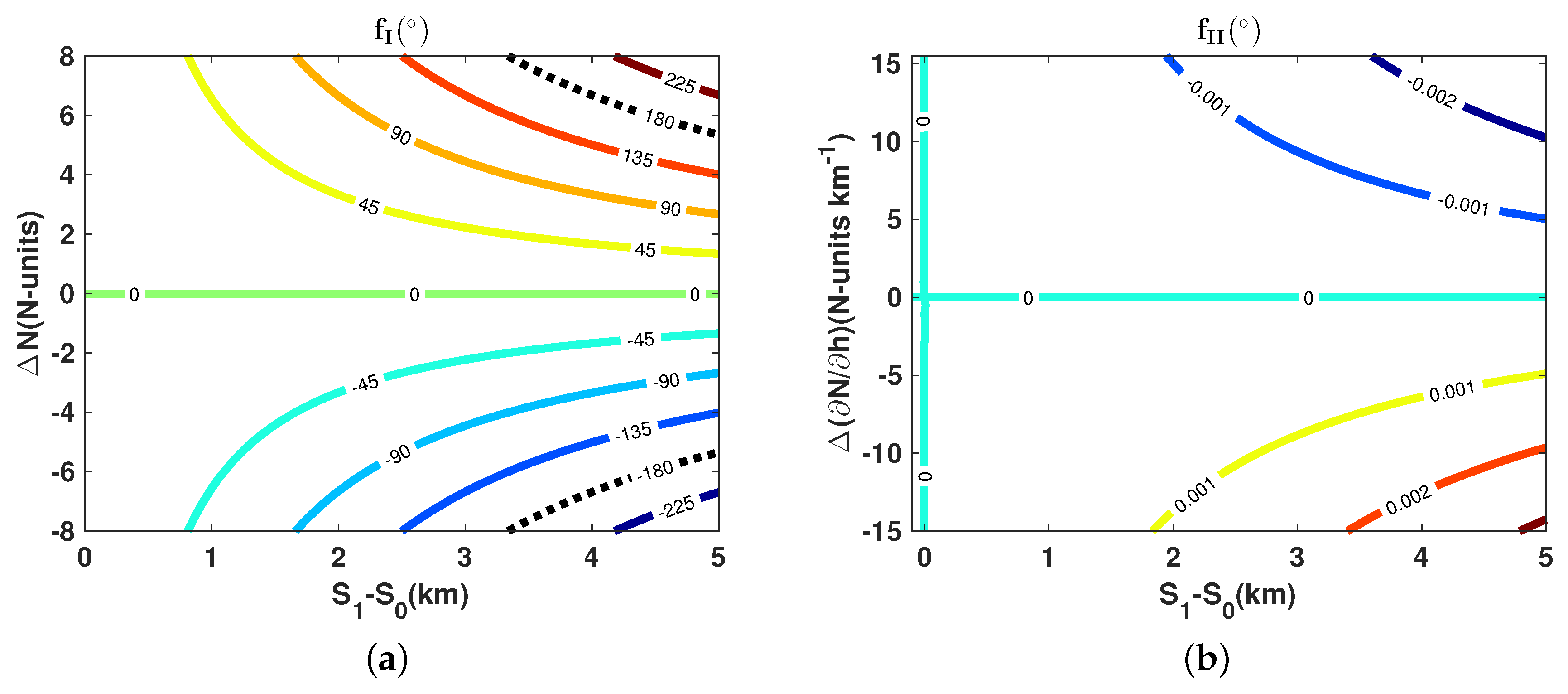
The first term, , matches the term retrieved in [17] and it is related to the variation of the mean refractive index along the ray path at the radar height between targets and and times and , . The second term, , takes into account the variations of the ray path length to targets and between and due to the change of the propagation conditions:
Figure A1a–d shows the contribution to the phase variation of and . Figure A1a show the contribution of as a function of the arc distance between targets and the variation of the mean horizontal refractivity. Since variations with are negligible, the results in Figure A1a have been obtained for N-units km. On the other hand, Figure A1b–d shows the contribution of as a function of the mean refractivity at time , the variation of the refractivity vertical gradient from to and the arc distance between targets (in Figure A1b, the mean refractivity is set to 340 N-units. In Figure A1c, the arc distance between targets is set to 5 km and in Figure A1d the vertical gradient is set to 15 N-units km).
The contribution of to the phase variation is around times the contribution of ; therefore, it will be neglected.
Figure A1.
Contribution of the horizontal term to the total phase variation. (a) as a function of the arc distance between both targets and the horizontal mean refractivity variation in the path. The vertical gradient is set to −157 N-units km−1. The dotted black line represents the maximum joint variation of refractivity and arc distance between targets to ensure a correct unwrapping of the phase; (b) as a function of the arc distance between both targets and the vertical gradient variation. The absolute averaged refractivity is set to 340 N-units; (c) as a function of the horizontal mean refractivity and the vertical gradient variation. The arc distance between both targets is set to 5 km; (d) as a function of the arc distance between both targets and the horizontal mean refractivity. The vertical gradient variation is set to 15 N-units km−1.


Appendix A.2. Vertical Contribution
The refractivity vertical gradient contributes to the total phase variation with a term that can be expressed as the sum of , which depends on the variation of the refractivity vertical gradient, the heights of the targets and their range, and which also depends on the refractivity vertical gradient at and the path length variation to and between and :
Figure A2a–d and Figure A3a–d show the contributions of and to as a function of the height difference between targets, the range difference between them and the refractivity vertical gradient variation.
Figure A2.
Contribution of to the total phase variation. (a) as a function of the vertical gradient variation and the height difference between targets. The arc distance from the radar to the first target and between targets are respectively set to 20 and 5 km; (b) as a function of the arc distance and the height variations between targets. The vertical gradient variation is set to 15 N-units km; (c) as a function of the vertical gradient variation and the arc distance between targets with a height difference between targets of 200 m; (d) as in (c), but setting the height difference to 150 m.

Height differences up to 200 m and arc distances between targets up to 5 km have been used. Furthermore, the distance from the radar to the first target was set to 20 km. Both and depend on , however this dependence is very weak. Therefore, the refractivity vertical gradient at has been set to N-units km. Figure A2c shows how the phase variation would wrap for refractivity vertical gradients of ±15 N-units km and height differences between targets of 200 m even for nearby targets. Figure A2d shows that for height and arc distance variations lower than 150 m and 2.2 km respectively, the phase variation would be correctly unwrapped.
Figure A3.
Contribution of to the total phase variation. (a) as a function of the vertical gradient variation and the height difference between targets. The arc distance from the radar to the first target and between targets are respectively set to 20 and 5 km; (b) as a function of the arc distance and the height variations between targets. The vertical gradient variation is set to 15 N-units km; (c) as a function of the vertical gradient variation and the arc distance between targets. The height difference between the targets is set to 200 m; (d) as a function of the absolute vertical gradient and the height difference between targets. The arc distance from the radar to the first target and between targets are respectively set to 20 and 5 km, and the vertical gradient variation is set to 15 N-units km.

Appendix A.3. Earth’s Curvature Contribution
Finally, the contribution of the Earth’s curvature term can also be expressed as the sum of two terms: and . depends on the time variation of the refractivity vertical gradient, the arc distance between targets and the height difference between them. also depends on the refractivity vertical gradient at time and the path length variation to and between and :
Figure A4.
Contribution of the Earth’s curvature term to the total phase variation. (a) as a function of the vertical gradient variation and arc distance between targets. The height difference between targets is set to 200 m; (b) as a function of the vertical gradient variation and the height difference between targets. The arc distance from the radar to the first target and between targets are respectively set to 20 and 5 km; (c) as a function of the arc distance and the height variations between targets. The vertical gradient variation is set to 15 N-units km; (d) as a function of the absolute vertical gradient and the arc distance between targets. The height difference between targets and the vertical gradient variation are set to 200 m and 15 N-units km, respectively.

Figure A4a–c shows the joint contribution of both terms to the total phase variation as a function of the arc distance and height variations between targets and the refractivity vertical gradient variation. Again, height differences and arc distances between targets up to 200 m and 5 km have been considered, and a refractivity vertical gradient at of N-units km has been assumed. Figure A4b,c shows that the Earth’s curvature term is not affected by the height difference between targets. In Figure A4d, the contribution of the Earth’s curvature term as a function of the refractivity vertical gradient at time is shown. Clearly, higher contributions are found for ducting and sub-refractive conditions.
Comparison of the Earth’s curvature and the vertical gradient terms shows that the contribution of the Earth’s curvature term to the phase variation is generally significantly lower than the contribution of the vertical gradient term. For example, for a height difference between targets of 200 m and an arc distance of 5 km, the vertical gradient term is approximately 30 times higher than the Earth’s curvature term. However, because the Earth’s curvature term does not depend on the height difference between targets while the vertical gradient term strongly depends on it, when the targets are placed at similar heights, the Earth’s curvature term can be higher than the vertical gradient term. In this case, as the height difference between targets decreases, the contribution of the vertical terms to the total phase variation in Equation (10) becomes negligible. Then, the contribution of the Earth’s curvature terms should be compared to the contribution of . For an extreme situation, with a zero mean refractivity variation at the targets height but a high refractivity vertical gradient variation of N-units km, the contribution of the Earth’s curvature term, if neglected would cause an error in the estimation of the variation of the mean refractivity of only 0.327 N-units for two targets separated an arc distance of 5 km. Therefore, the Earth’s curvature contribution to the phase variation between consecutive PPIs can also be neglected.
References
- Weckwerth, T.M.; Wilson, J.W.; Wakimoto, R.M. Thermodynamic variability within the convective boundary layer due to horizontal convective rolls. Mon. Weather Rev. 1996, 124, 769–784. [Google Scholar] [CrossRef]
- Ziegler, C.L.; Lee, T.J.; Pielke, R.A. Convective initiation at the dryline: A modeling study. Mon. Weather Rev. 1997, 125, 1001–1026. [Google Scholar] [CrossRef]
- Crook, N.A. Sensitivity of moist convection forced by boundary layer processes to low-level thermodynamic fields. Mon. Weather Rev. 1996, 124, 1767–1785. [Google Scholar] [CrossRef]
- Weckwerth, T.M. The effect of small-scale moisture variability on thunderstrom initiation. Mon. Weather Rev. 2000, 128, 4017–4030. [Google Scholar] [CrossRef]
- Deeter, M.N.; Evans, K.F. Mesoscale variations of water vapor inferred from millimeter-wave imaging radiometer during TOGA COARE. J. Appl. Meteorol. Notes Corresp. 1997, 36, 183–188. [Google Scholar] [CrossRef]
- Dabberdt, W.F.; Schlatter, T.W. Research Opportunities from Emerging Atmospheric Observing and Modeling Capabilities. Bull. Am. Meteorol. Soc. 1996, 77, 305–323. [Google Scholar] [CrossRef] [Green Version]
- Weckwerth, T.M.; Pettet, C.R.; Fabry, F.; Park, S.; LeMone, M.A.; Wilson, J.W. Radar refractivity retrieval: validation and application to shrot-term forecasting. J. Appl. Meteorol. 2005, 44, 285–300. [Google Scholar] [CrossRef]
- Fabry, F. The Spatial Variability of Moisture in the Boundary Layer and its Effect on Convection Initiation: Project-Long Characterization. Mon. Weather Rev. 2006, 134, 978–987. [Google Scholar] [CrossRef]
- Matzler, C. Parabolic Equations for Wave Propagation and the Advanced Atmospheric Effects Prediction System; Institute of Applied Physics, University of Bern: Bern, Switzerland, 2004. [Google Scholar]
- Levy, M.F. Horizontal parabolic equation solution of radiowave propagation problems on large domains. IEEE Trans. Antennas Propag. 1995, 43, 137–144. [Google Scholar] [CrossRef]
- Barrios, A.E. A terrain parabolic equation model for propagation in the troposphere. IEEE Trans. Antennas Propag. 1994, 42, 90–98. [Google Scholar] [CrossRef]
- Dockery, G.D. Modeling electromagnetic wave propagation in the troposphere using the parabolic equation. IEEE Trans. Antennas Propag. 1988, 36, 1464–1470. [Google Scholar] [CrossRef]
- Ozgun, O. Recursive two-way parabolic equation approach for modeling terrain effects in tropospheric propagation. IEEE Trans. Antennas Propag. 2009, 57, 2706–2714. [Google Scholar] [CrossRef]
- Liang, Y.C.; Chen, K.C.; Li, Y.G.; Mahonen, P. Cognitive Radio Networking and Communications: An overview. IEEE Trans. Veh. Technol. 2011, 60, 3386–3407. [Google Scholar] [CrossRef]
- Bevis, M.; Businger, S.; Herring, T.A.; Rocken, C.; Anthes, R.A.; Ware, R.H. GPS Meteorology: Remote Sensing of Atmospheric Water Vapor Using the Global Positioning System. J. Geophys. Res. 1992, 97, 15787–15801. [Google Scholar] [CrossRef]
- Businger, S.; Chriswell, S.; Bevis, M.; Duan, J.; Anthes, R.; Rocken, C.; Ware, H.; Exner, M.; VanHove, T.; Solheim, F. The Promise of GPS in Atmospheric Monitoring. Bull. Am. Meteorol. Soc. 1996, 77, 5–18. [Google Scholar] [CrossRef] [Green Version]
- Fabry, F.; Frush, C.; Zawadzki, I.; Kilambi, A. On the extraction of near-surface index of refraction using radar phase measurements from ground targets. J. Atmos. Ocean. Technol. 1997, 14, 978–987. [Google Scholar] [CrossRef]
- Fabry, F. Meteorological Value of Ground Target Measurements. J. Atmos. Ocean. Technol. 2004, 21, 560–573. [Google Scholar] [CrossRef]
- Weckwerth, T.M.; Parson, D.B.; Koch, S.E.; Moore, J.A.; LeMone, M.A.; Demoz, B.B.; Flamant, C.; Geerts, B.; Wang, J.; Feltz, W.F. An overview of the International H2O Project (IHOP_2002) and some preliminary highlights. Bull. Am. Meteorol. Soc. 2004, 85, 253–277. [Google Scholar] [CrossRef]
- Roberts, R.D.; Fabry, F.; Kennedy, P.C.; Nelson, E.; Wilson, J.; Rehak, N.; Fritz, J.; Chandrasekar, V.; Braun, J.; Sun, J.; et al. REFRACTT_2006: Real-Time retrieval of high-resolution low-level moisture fields from operational NEXRAD and research radars. Bull. Am. Meteorol. Soc. 2008, 89, 1535–1548. [Google Scholar] [CrossRef]
- Bodine, D.; Heinselman, P.L.; Cheong, B.L.; Michaud, D.; Palmer, R.D. A case study on the impact of Moisture Variability on Convection Initiation using Radar Refractivity Retrievals. J. Appl. Meteorol. Climatol. 2010, 49, 1766–1778. [Google Scholar] [CrossRef]
- Bodine, D.; Michaud, D.; Palmer, R.D.; Heinselman, P.L.; Brotzge, J.; Gasperoni, N.; Cheong, B.L.; Xue, M.; Gao, J. Understanding Radar Refractivity: Sources of Uncertainty. J. Appl. Meteorol. Climatol. 2011, 50, 2543–2560. [Google Scholar] [CrossRef] [Green Version]
- Nicol, J.C.; Illingwoth, A.; Darlington, T.; Kitchen, M. Quantifying Errors due to Frequency Changes and Target Location Uncertainty for Radar refractivity Retrievals. J. Atmos. Ocean. Technol. 2013, 30, 2006–2024. [Google Scholar] [CrossRef]
- Parent du Chatelet, J.; Tabary, P.; Boudjabi, C. Evaluation of the refractivity measurement feasibility with a C-Band radar equipped with a magnetron transmitter. In Proceedings of the 33rd International Conference on Radar Meteorology, Cairns, Australia, 6–10 August 2007. [Google Scholar]
- Besson, L.; Boudjabi, C.; Caumont, O.; Parent du Chatelet, J. Links between Weather Phenomena and Characterisitcs of Refractivity Measured by Precipitation Radar. Bound. Layer Meteorol. 2011, 143, 77–95. [Google Scholar] [CrossRef]
- Nicol, J.C.; Illingwoth, A.; Bartholomew, K. The potential of 1h refractivity changes from an operational C-Band magnetron-based radar for numerical weather prediction validation and data assimilation. Q. J. R. Meteorol. Soc. 2014, 140, 1209–1218. [Google Scholar] [CrossRef]
- Cheong, B.L.; Palmer, R.; Chandrasekar, V.; Junyent, F. Real-time Refractivity Retrieval Using the Magnetron-based CASA X-band Radar Network during the Spring 2008 Campaign. In Proceedings of the International Geoscience and Remote Sensing Symposium (IGARSS), Boston, MA, USA, 6–11 July 2008. [Google Scholar]
- Cheong, B.L.; Palmer, R.; Curtis, C.D.; Yu, T.Y.; Zrnic, D.S.; Forsyth, D. Refractivity Retrieval Using the Phased-Array Radar: First Results and Potencial for Multimission Operation. IEEE Trans. Geosci. Remote Sens. 2008, 46, 2527–2537. [Google Scholar] [CrossRef]
- Parent du Chatelet, J.; Boudjabi, J.; Boudjabi, C. A new formulation for signal reflected from a target using a magnetron radar. In Proceedings of the ERAD 2008—The 5th European Conference on Radar in Meteorology and Hydrology, Helsinki, Finland, 30 June–4 July 2008. [Google Scholar]
- Junyent, F.; Chandrasekar, V.; McLaughlin, D.; Insanic, E.; Bharadwaj, N. The CASA Integrated Project 1 Networked Radar System. J. Atmos. Ocean. Technol. 2010, 27, 61–78. [Google Scholar] [CrossRef]
- Parent du Chatelet, J.; Boudjabi, C.; Besson, L.O.C. Errors caused by long-term drifts of magnetron frequencies for refractivity measurement with a radar: Theoretical formulation and initial validation. J. Atmos. Ocean. Technol. 2012, 29, 1428–1434. [Google Scholar] [CrossRef]
- Nicol, J.C.; Illingwoth, A. The effect of Phase-Correlated Returns and Spatial Smoothing on the Accuracy of Radar Refractivity Retrievals. J. Atmos. Ocean. Technol. 2013, 30, 22–39. [Google Scholar] [CrossRef]
- Besson, L.; Parent du Chatelet, J. Solutions for Improving the Radar Refractivity Measurements by taking Operational Constraints into Account. Bound. Layer Meteorol. 2013, 30, 1730–1742. [Google Scholar] [CrossRef]
- Rogers, L.T.; Hattan, C.; Stapleton, J. Estimating evaporation duct heights from radar sea echo. Radio Sci. 2000, 35, 955–966. [Google Scholar] [CrossRef] [Green Version]
- Gerstoft, P.; Rogers, L.; Krolik, J.L.; Hodgkiss, W. Inversion for refractivity parameters from radar sea clutter. Radio Sci. 2003, 38. [Google Scholar] [CrossRef] [Green Version]
- Zhao, X.; Huang, S. Estimation of atmospheric duct structure using radar sea clutter. J. Atmos. Sci. 2012, 69, 2808–2818. [Google Scholar] [CrossRef]
- Karimian, A.; Yardim, C.; Gerstoft, P.; Hodgkiss, W.; Barrios, A.E. Refractivity estimation from sea clutter: An invited review. Radio Sci. 2011, 46. [Google Scholar] [CrossRef] [Green Version]
- Park, S.; Fabry, F. Simulation and interpretation of the phase data used by radar refractivity retrieval algorithm. J. Atmos. Ocean. Technol. 2010, 27, 1286–1301. [Google Scholar] [CrossRef]
- Park, S.; Fabry, F. Estimation of Near-Ground Propagation Conditions using Radar Ground Echo Coverage. J. Atmos. Ocean. Technol. 2011, 28, 165–180. [Google Scholar] [CrossRef]
- Feng, Y.; Fabry, F.; Weckwerth, T.M. Improving Radar Refractivity Retrieval by considering the change in the Refractivity Profile and the Varying Altitudes of Ground Targets. J. Atmos. Ocean. Technol. 2016, 33, 989–1004. [Google Scholar] [CrossRef]
- ITU-R, P.; 453-11, R. The Radio Refractive Index: Its Formula and Refractivity Data. 2015. Available online: https://www.itu.int/dmspubrec/itu-r/rec/p/R-REC-P.453-11-201507-S!!PDF-E.pdf (accessed on 6 June 2018).
- UCAR/NCAR. Earth Observing Laboratory. S-Band/Ka-Band Polarimetric (S-PolKa) Data cfRadial Format. Version 1.0. UCAR/NCAR—Earth Observing Laboratory. 1996. Available online: https://doi.org/10.5065/D6WW7FV6 (accessed on 11 January 2015).
- Lutz, J.P.; Lewis, E.; Loew, E.; Randall, M.; Van Andel, J. NCAR SPol: Portable polarimetric S-Band radar. In Proceedings of the Preprints, Ninth Symposium on Meteorological Observations and Instrumentation, Charlotte, NC, USA, 27–31 March 1995; pp. 408–410. [Google Scholar]
- Bean, B.R.; Dutton, E.J. Radio Meteorology. In National Bureau of Standards Monograph; National Bureau of Standards: Gaithersburg, MD, USA, 1968; 435p. [Google Scholar]
- Doviak, R.J.; Zrnic, D.S. Doppler Radar and Weather Observations, 2nd ed.; Academy Press Inc.: Cambridge, MA, USA, 2006; 562p. [Google Scholar]
- Ferreti, A.; Prati, C.; Rocca, F. Permanent scatterers in SAR interferometry. IEEE Trans. Geosci. Remote Sens. 2001, 39, 8–20. [Google Scholar] [CrossRef] [Green Version]
- Noferiny, L.; Pieraccini, D.; Mecatti, D.; Luzi, G.; Atzeni, C.; Tambburini, A.M.B. Permanent Scatterers Analysis for Atmospheric Correction in Ground-Based SAR Interferometry. IEEE Trans. Geosci. Remote Sens. 2005, 43, 1459–1470. [Google Scholar] [CrossRef]
Figure 1.
Location of the study area at the base of the Rocky Mountains in Boulder (Northeast Colorado, USA): (a) Google Earth™ image showing the location of the radar and the automatic weather stations; (b) topographic map of the terrain (National Elevation Dataset of the U. S. Geological Survey (USGS)).

Figure 2.
Radar backscattered power: (a) 0∘ elevation angle; (b) 0.5∘ elevation angle.

Figure 3.
Geometry between the Earth’s surface and the ray path taking into account the vertical gradient of the refractivity. (a) ray path in a spherically stratified atmosphere along the Earth’s surface; (b) straight path of the ray above the equivalent Earth of radius ae.
Figure 3.
Geometry between the Earth’s surface and the ray path taking into account the vertical gradient of the refractivity. (a) ray path in a spherically stratified atmosphere along the Earth’s surface; (b) straight path of the ray above the equivalent Earth of radius ae.

Figure 4.
(a–c) meteorological observations; (d) refractivity derived from automatic weather stations (blue and red lines represent data from Foothills and Mesa weather stations, respectively); (e) refractivity vertical gradient estimated from the difference in refractivity measurements at the Mesa and Foothills locations.

Figure 5.
Resolution area defined by the targets in Mesa and Foothills azimuths.

Figure 6.
Mean refractivity variation at the radar height, absolute mean refractivity at the weather station heights and refractivity vertical gradient obtained from radar phase measurements (red) and weather stations data (blue) in the Mesa and Foothills areas.
Figure 6.
Mean refractivity variation at the radar height, absolute mean refractivity at the weather station heights and refractivity vertical gradient obtained from radar phase measurements (red) and weather stations data (blue) in the Mesa and Foothills areas.

Figure 7.
Mean refractivity variation at the radar height and refractivity vertical gradient variation obtained from radar phase measurements at the Eldorado test area.
Figure 7.
Mean refractivity variation at the radar height and refractivity vertical gradient variation obtained from radar phase measurements at the Eldorado test area.


Table 1.
Technical specifications of the S-Pol Radar and operational parameters used in the experiment.
Table 1.
Technical specifications of the S-Pol Radar and operational parameters used in the experiment.
| Parameter | Value |
|---|---|
| Frequency | 2.8 GHz |
| Wavelength | 10 cm |
| Pulse-width | 0.994 s |
| Pulse repetition frequency (PRF) | 655–714 Hz |
| Range resolution | 150 m |
| Beam-width | 0.918 |
| Scan-rate | 11.13–12.14s |
| Samples | 54 |
| Scanning elevation angle | 0–0.5 |
| Noise Power | dBm |
Table 2.
Location parameters of the S-Pol Radar and the weather stations.
| Station | Longitude | Latitude | Altitude (m) | Distance to Radar (km) | Azimuth () | Gate |
|---|---|---|---|---|---|---|
| S-pol Radar | 10511′42 W | 3957′00 N | 1742 | – | – | – |
| Mesa | 10516′42 W | 3958′48 N | 1885 | 7.578 | 295.9 | 51 |
| Foothills | 10514′35 W | 4001′48 N | 1625 | 9.777 | 335.3 | 69 |
Table 3.
Radar and automatic weather stations information.
| Source | Data Collecting Time (UTC) | Samples | Resolution |
|---|---|---|---|
| Radar | 0000 to 2215 on 1 August 2006 | 356 PPIs | <4 min |
| Weather Stations | 267 Observations (T, p and e) | 5 min |
Table 4.
RMSE and BIAS of mean refractivity variation estimates and refractivity vertical gradient variations at the radar height and at the Mesa and Foothills locations.
Table 4.
RMSE and BIAS of mean refractivity variation estimates and refractivity vertical gradient variations at the radar height and at the Mesa and Foothills locations.
| Estimator | Parameter | Mesa | Foothills |
|---|---|---|---|
| N () | RMSE | 1.91 | 1.79 |
| BIAS | |||
| N () | RMSE | 1.65 | 3.00 |
| BIAS | 0.68 | ||
| RMSE | 15.37 | 15.90 | |
| BIAS | 10.50 | 10.67 |
© 2018 by the authors. Licensee MDPI, Basel, Switzerland. This article is an open access article distributed under the terms and conditions of the Creative Commons Attribution (CC BY) license (http://creativecommons.org/licenses/by/4.0/).
Share and Cite
MDPI and ACS Style
López, R.N.; Río, V.S.d. High Temporal Resolution Refractivity Retrieval from Radar Phase Measurements. Remote Sens. 2018, 10, 896. https://doi.org/10.3390/rs10060896
AMA Style
López RN, Río VSd. High Temporal Resolution Refractivity Retrieval from Radar Phase Measurements. Remote Sensing. 2018; 10(6):896. https://doi.org/10.3390/rs10060896
Chicago/Turabian StyleLópez, Rubén Nocelo, and Verónica Santalla del Río. 2018. "High Temporal Resolution Refractivity Retrieval from Radar Phase Measurements" Remote Sensing 10, no. 6: 896. https://doi.org/10.3390/rs10060896
Note that from the first issue of 2016, this journal uses article numbers instead of page numbers. See further details here.