Article

Integration of Single-Frequency GNSS and Strong-Motion Observations for Real-Time Earthquake Monitoring

1
National Time Service Center, Chinese Academy of Sciences, Shu Yuan Road, Xi’an 710600, China
2
University of Chinese Academy of Sciences, Yu Quan Road, Beijing 100049, China
3
Key Laboratory of Precision Navigation Positioning and Timing Technology, Chinese Academy of Sciences, Xi’an 710600, China
*
Author to whom correspondence should be addressed.
Remote Sens. 2018, 10(6), 886; https://doi.org/10.3390/rs10060886
Submission received: 18 April 2018 / Revised: 26 May 2018 / Accepted: 5 June 2018 / Published: 6 June 2018

Abstract

:
In this study, a real-time earthquake monitoring system based on the integration of single-frequency global navigation satellite system (GNSS) and strong motion (SM) observations was developed. This high-precision integrated system can provide full-frequency monitoring information, and it makes full use of SM data to quickly and accurately determine the vibration window for initial baseline shift correction. High-precision displacement data obtained from GNSS epoch-differenced velocity estimation are used to constrain the SM’s low-frequency baseline shift. Hence, full-frequency monitoring information (displacement, velocity, and acceleration) can be provided in real-time. Three different datasets were used for validation and the results confirm that the proposed system can be used for practical earthquake monitoring.

Graphical Abstract

1. Introduction

Epoch-differenced velocity estimation technology, which is based on single-frequency global navigation satellite system (GNSS) observations and satellite broadcast ephemeris, has the advantages of no ambiguity parameters, rapid initialization, high precision, low cost, and rapid turnaround; therefore, it is widely used in earthquake engineering applications, such as real-time earthquake monitoring, early warning, and rapid response [1]. In addition, other studies have focused on GNSS positioning from mass-market receivers for monitoring purposes and real-time earthquake monitoring activities [2,3,4,5]. Meng et al. used GNSS positioning technology for structural health monitoring and geo-hazard early warning [2], Bellone et al. and Dabove and Li et al. also used the low-cost receiver for fast deformation monitoring (e.g., earthquakes) [3,4,5]. However, owing to its low sampling rate, the GNSS can only provide low-frequency displacement information with high precision; high-frequency information, such as velocity and acceleration, is significantly affected by noise [6,7,8].
Strong motion (SM) data, which is inexpensive, can provide high-frequency information with high precision and high sensitivity; however, the integrated velocity and displacement are seriously distorted owing to a baseline shift caused by low-frequency noise and tilting or rotation of the instrument; consequently, the recovered displacement has a precision of the order of decimeters or worse [9,10,11,12,13,14].
The effective integration of GNSS and SM data to maximise their complementary advantages is a topic of significant research interest [14,15]. The goal is to develop an early warning system that not only provides high-precision and full-frequency information, but is also inexpensive and efficient. Wang et al. used linear trigonometric and time correlation to express the baseline shift of SM data and to correct the displacement to be consistent with the high-frequency GNSS displacement using a least-squares solution [14]. This method constrains the baseline shift and results in high-precision velocity and displacement measurements; however, the assumptions of the linear function are influenced by subjective factors and, therefore, it cannot be employed for real-time applications. Bock et al. used a Kalman filter to realise the combination of GNSS and SM [15]. The inputs are the GNSS’ displacement and the SM’s acceleration; the outputs are the filtered displacement and velocity. The Kalman filter approach can result in high precision and broadband displacement information. However, GNSS uses a precise positioning mode that requires a dual-frequency receiver and high-precision satellite ephemeris, with associated expense and poor turnaround time; hence, the widespread implementation of this approach is limited. Tu et al. proposed an approach to compare the difference between the global positioning system (GPS) displacement and SM-integrated displacement to derive the baseline shift, and to subsequently recover the final displacement and velocity [16]. However, validation trials on an experimental dataset indicate that it worked only for 50 Hz GPS data, which limits the method’s practical application. Subsequently, many researchers have studied the tight integration of high-quality dual-frequency GNSS and SM observations for deformation monitoring and earthquake early warning systems [16,17,18,19,20,21,22,23,24,25,26], which have the advantages of being complementary systems; however, they have the drawback of significant cost. Only a few researchers have strongly considered the cost issues (e.g., Saunders et al. [26]) by using single-frequency GPS and low-cost MEMS accelerometers for earthquake early warning and rapid response.
In this context, our study proposes a real-time earthquake monitoring system based on the integration of a single-frequency GNSS and low-cost SM observations. The system is composed of three modules, all of which work in real time: data input, processing, and output. The system uses a Kalman filter method to combine the complementary systems and allow real-time retrieval of velocity and acceleration information for applications in earthquake monitoring and early warning.

2. Methodology

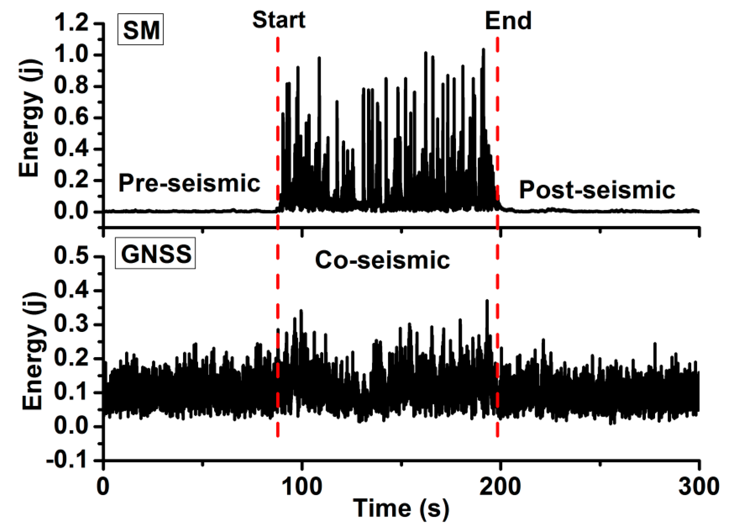
2.1. Determination of the Signal Window

High-frequency GNSS has issues such as high levels of noise, time-consuming separation of the true vibration signal from the noise, and poor real-time sensitivity. However, high-sensitivity SM detectors can determine the signal window quickly and accurately, which is useful for initialization and quality inspection.
A seismic event can be divided into three periods: pre-seismic, co-seismic, and post-seismic. For the time series of the co-seismic acceleration, we define an average energy function:
W n = 1 N ( t = n + 1 t = n + N | a ( t ) | Δ t 2 ) , W 0
where W n is the average energy at epoch n ,   W 0 is the rest energy,   N is the epoch numbers to calculate the average energy, a ( t ) is the acceleration time series, and Δ t is the sample interval. The signal start time t 1 is defined as the time when the average energy W n is more than five times the rest energy W 0 ; the end time t 2 is defined as the time after the start time when the average energy W n is less than five times the rest energy W 0 .
Figure 1 shows a comparison of average energies for GNSS and SM. The GNSS energy function has high levels of noise and, thus, cannot be used to accurately determine the signal start and end times. Consequently, it is unsuitable for real-time initialization of the GNSS velocity shifts, making implementation for earthquake monitoring and early warning in real-time difficult. However, the shaking window can be readily determined from the SM energy function, and it complements the GNSS system for the initialization shift before the earthquake and quality evaluation after the earthquake.

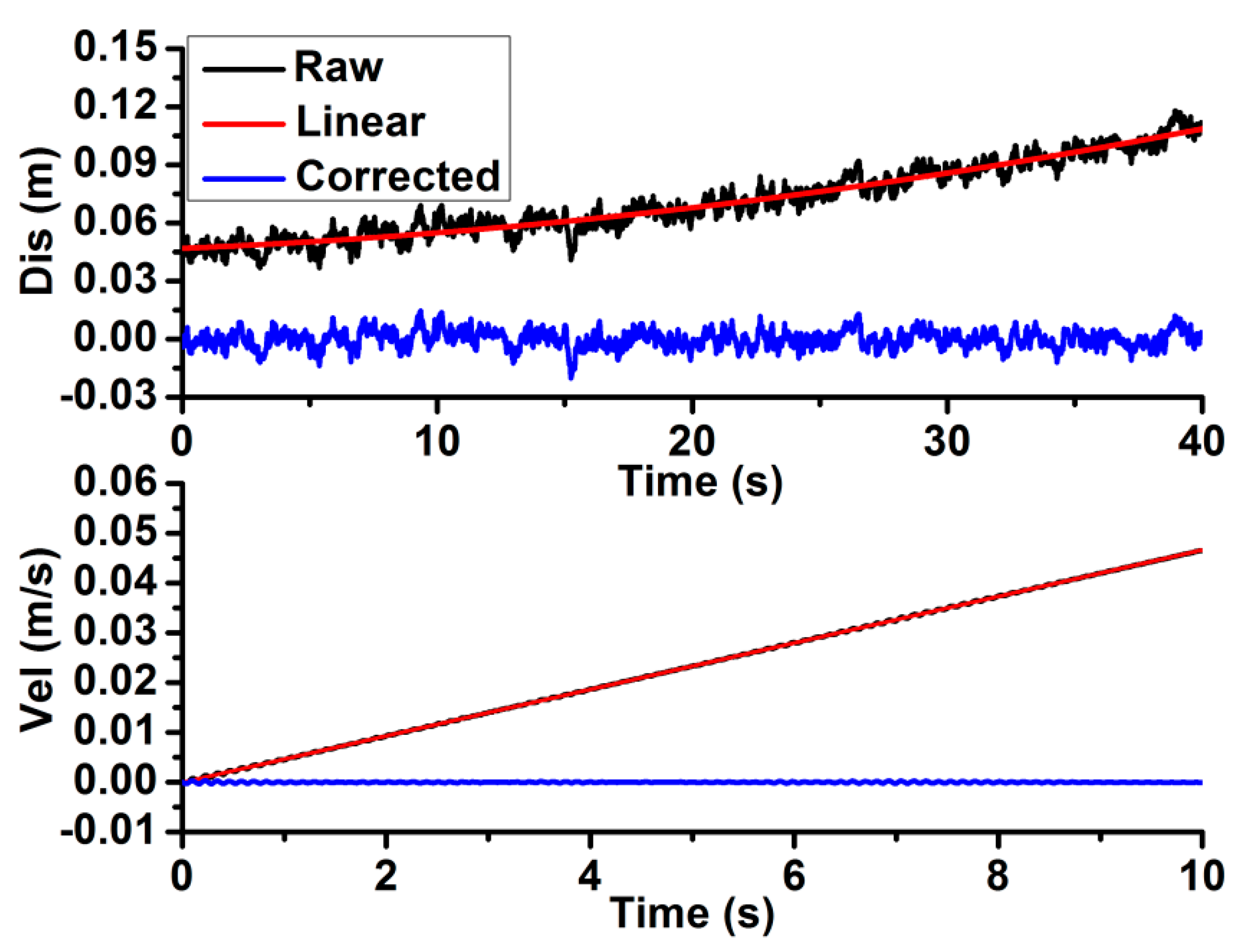
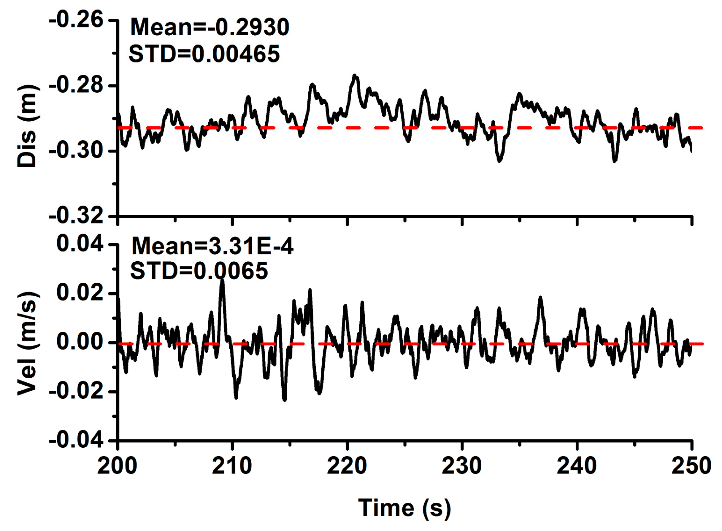
2.2. Initial Baseline Shift Correction of the Integrated System before an Earthquake

Colosimo et al. and Tu et al. reported a linear shift in the estimated velocity in epoch difference calculations due to uncorrected atmosphere errors; this shift is stable over a period of around 10 min [1,16]. One to two minutes of velocity data prior to the earthquakes was selected to determine the initial shift by assuming that the time series of the GNSS velocity v ( t ) can be expressed as:
v ( t ) = ( v 1 ,   v 2 ,   v 3 v N ) .
Given the presence of high-frequency noise, we usually integrate the velocity to obtain low-frequency displacement and use least-squares fitting to estimate the initial shift. Equations (3) and (4) are the solution and correction, respectively, for the displacement:
s ( t ) = ( s 1 ,   s 2 ,   s 3 s N ) = At 2 + Bt + C ,
v c ( t ) = v ( t ) ( 2 A ^ t + B ^ ) ,
where s ( t ) is the integrated displacement time series, A ,   B ,   and   C are the polynomial fitting coefficients, and v c ( t )   is the corrected velocity.
The SM acceleration is corrected by a constant initial baseline shift to compensate for environmental noise and instrument effects. The time series of the acceleration can be written as:
a ( t ) = ( a 1 ,   a 2 ,   a 3 a N )
Similarly, the acceleration integrated to velocity or displacement used least-squares fitting to solve the acceleration initial shift correction:
a c ( t ) = a ( t ) a ^ ( t ) ,
where a c ( t ) is the corrected acceleration and a ^ ( t ) is the initial shift correction for acceleration. Figure 2 shows the GNSS and SM system’s initial baseline shift corrections. After correction, the GNSS velocity data fluctuate around the zero line, implying that the initial baseline shift correction model is objective and accurate.

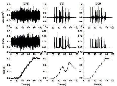
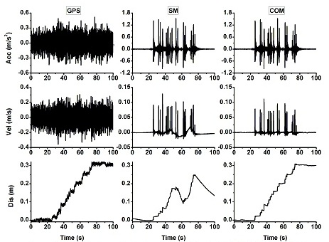
2.3. Integration during an Earthquake

Low-frequency displacement can be accurately recovered from the GNSS single system’s velocity estimation and the initial shift correction [19]:
s c ( t ) = t = 1 t = N v c ( t ) Δ t = ( s c 1 ,   s c 2 ,   s c 3 s cN ) .
For the SM sensors, there is an additional instantaneous shift and new permanent shift due to the instrument’s tilting or rotation during the shaking. Although they can significantly distort the integrated velocity and displacement, the magnitude of these shifts is small (about 0.001 m / s 2 ) and can be ignored. An accurate acceleration can be obtained from:
a c ( t ) = ( a c 1 ,   a c 2 ,   a c 3 a cN ) .
The integrated system used a Kalman filter to determine velocity [15]. The GNSS’ displacement and SM’s acceleration were used for the inputs; the output is the accurate velocity information. The observation equations are:
Y ( t ) = A X ( t ) + ε Y ,
Y ( t ) = [ Y s ( t ) Y v ( t ) Y a ( t ) ] ,
A = [ 1 0 0 0 1 0 0 0 1 ] ,
X ( t ) = [ s ( t ) v ( t ) a ( t ) ] ,
ε Y N ( 0 ,   Q Y ) ,
P = Q Y 1 = [ 1 q s 1 q v 1 q a ] ,
where Y ( t ) denote the observation values, A is the coefficient matrix, X ( t ) denote the solution parameters,   ε Y is the observation noise, and Q Y is the noise variance matrix, P is the observation weight matrix, and q a ,   q v , and   q s are the noise variance of acceleration, velocity, and displacement, respectively.
The corresponding state equation can be written as:
X ( t ) = Φ X ( t 1 ) + ε s ,
Φ = [ 1 τ τ 2 2 0 1 τ 0 0 1 ] ,
  ε s N ( 0 ,   Q s ) ,
Q s = τ q a 2 [ τ 4 20 τ 3 8 τ 2 6 τ 3 8 τ 2 3 τ 2 τ 2 6 τ 2 1 ] ,
where Φ is the state transition matrix, ε s is the dynamic noise, Q s is the dynamic noise matrix, and τ is the sample interval of the acceleration.
The prediction estimation can be expressed as:
X ( t ) ¯ = Φ X ^ ( t 1 ) ,
Q ( t ) ¯ = Φ ( t 1 ) Q ( t 1 ) Φ T ( t 1 ) + Q s ( t 1 ) ,
and the filter estimation can be expressed as:
Q Y ( t ) = P 1 + A Q ( t ) ¯ A T ,
Q ( t ) = ( Q ( t ) ¯ 1 + A T Q Y 1 ( t ) A ) 1 ,
X ^ ( t ) = X ( t ) ¯ + Q ( t ) A T Q Y 1 ( t ) ( Y ( t ) A X ( t ) ¯ ) .
In the real-time filtering system, the predict estimation was carried out on the SM sample point, and the filter estimation was performed on the GNSS sample point. Hence, the integrated system can obtain high-precision displacement, velocity, and acceleration information in real-time.

2.4. Quality Assessment of the Integrated System

SM sensors can determine the signal end time quickly and accurately after shaking, perform quality control, and prepare for the next initialization. The inspection was performed separately for the GNSS system, where the time series of velocity were integrated into displacement to determine whether the permanent displacement was stable based on a criterion of standard deviation (STD) of less than 2 cm. On the other hand, for SM, the solved velocity is assessed by whether it returns to the zero level after shaking stops, using the threshold of STD less than 1 cm/s as the criterion.
Figure 3 is an example for the quality evaluation of the integrated system. The permanent displacement is stable and the velocity is on the zero level after the event, both of which indicate that the baseline shift is appropriate.

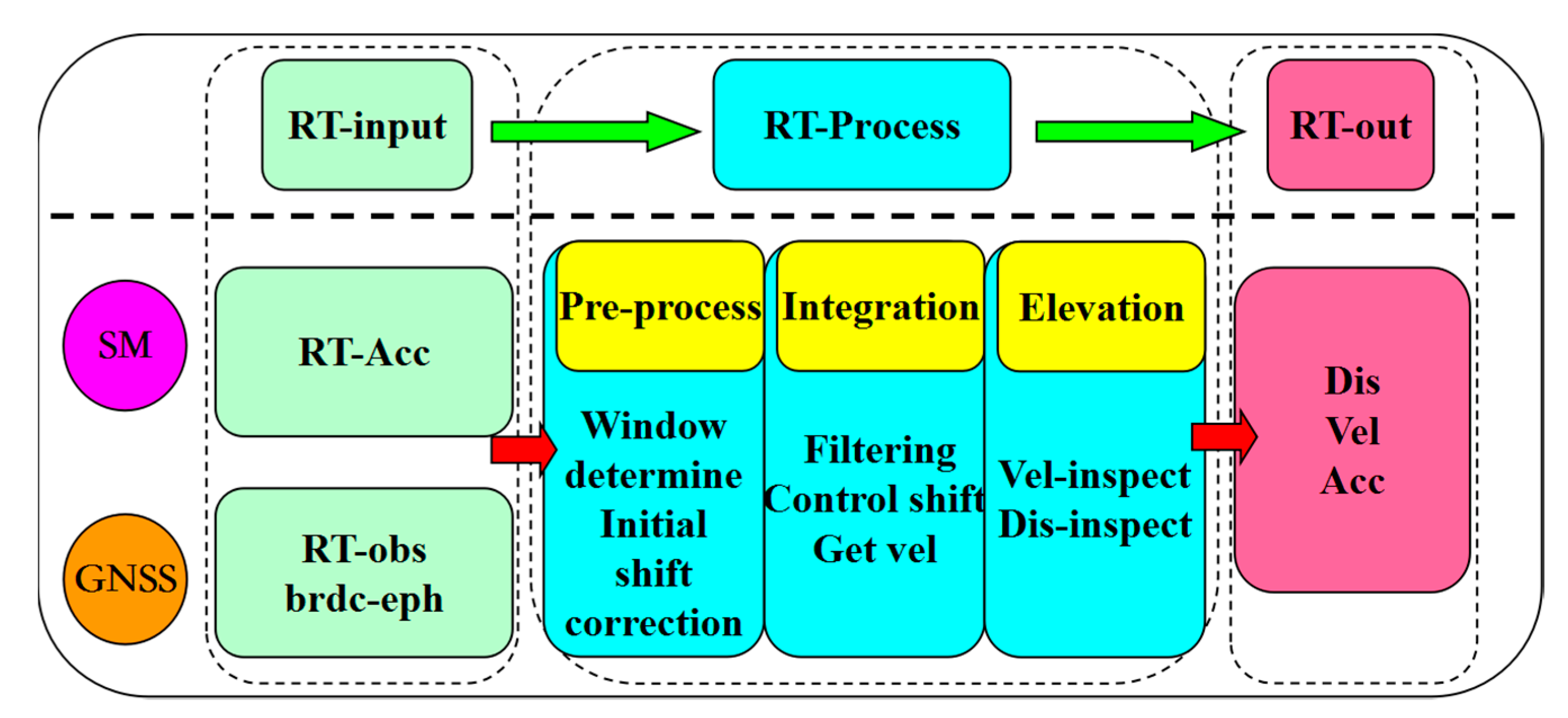
2.5. Implementation of the Real-Time Integrated System

The system is divided into three modules: real-time data stream input, real-time data processing, and output, it is shown in Figure 4.
(1)
The real-time data stream input module collects SM acceleration data, GNSS observation data, satellite broadcast ephemeris products, and associated parameters.
(2)
The real-time data processing module include pre-processing, integration, and quality control. During the pre-process period, after the SM determines the signal start, each subsystem carries out an initial shift correction. Then, the GNSS system provides accurate displacement information and the SM system provides accurate acceleration information. In the integration process period, the GNSS displacement and SM acceleration are the system inputs to the Kalman filter process; the accurate and low-frequency displacement can effectively constrain the SM’s baseline shift and retrieve high-precision velocity information. In the quality control module, the integrated system’s velocity and displacement are inspected; the accuracy and reliability are also verified.
(3)
The real-time output module controls the output of the displacement, velocity, acceleration, and accuracy information.

3. Validation Results and Analysis

The integrated system was tested and validated using three different datasets: (1) an experimental dataset including GPS and SM observations collected simultaneously on a dedicated experimental platform; (2) an experimental dataset with the BeiDou Satellite System (BDS) and SM observations collected simultaneously in a dedicated experimental setup; and (3) GPS and SM data collected from the E1 Mayor-Cucapah earthquake. All three datasets were processed in a simulated real-time mode by only using data up to the processed epoch and L1 single-frequency GNSS observations; velocity and acceleration were analysed by the combined system. In addition, all the scenarios which are examined in the experiments are not the transient component, but the co-seismic component of the ground response.

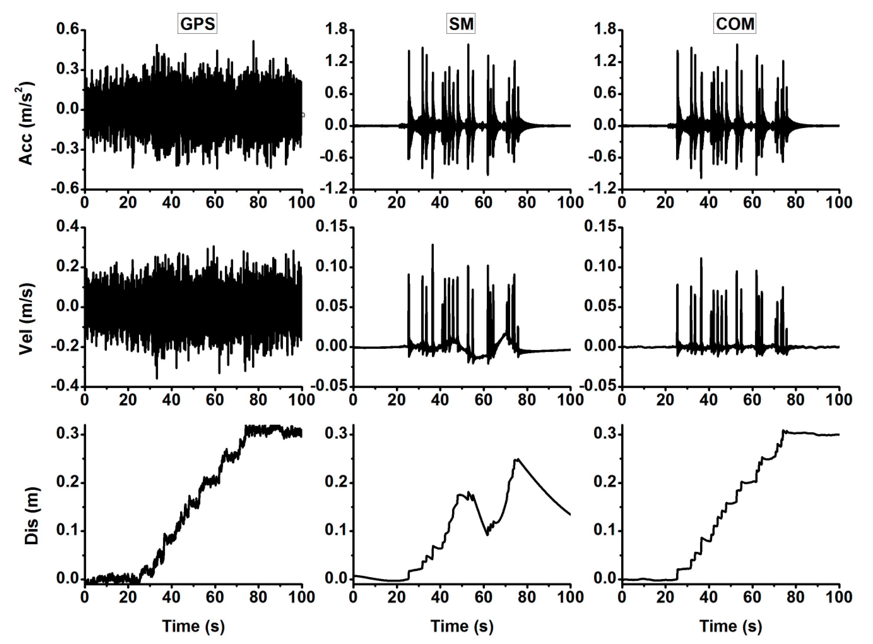
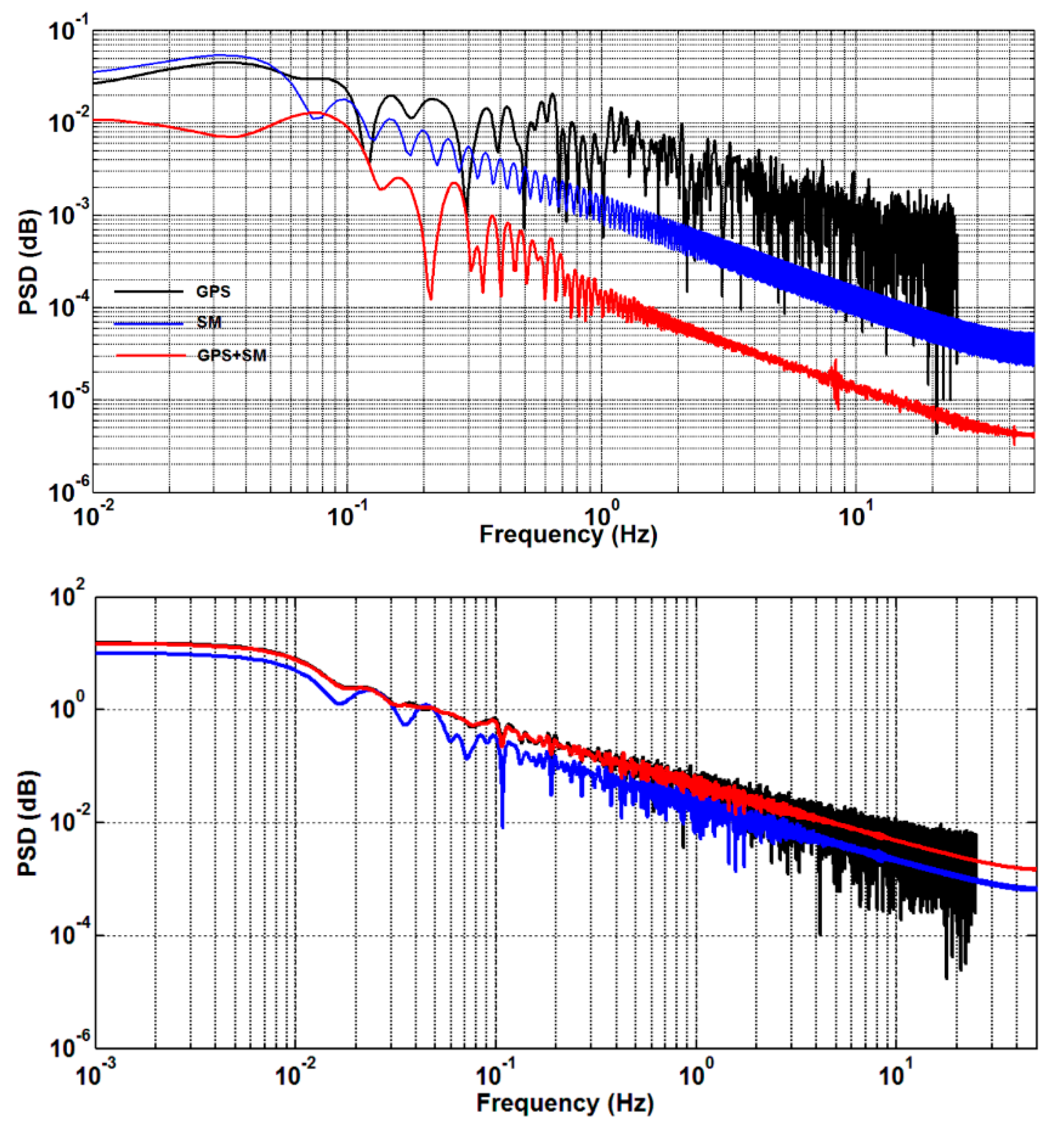
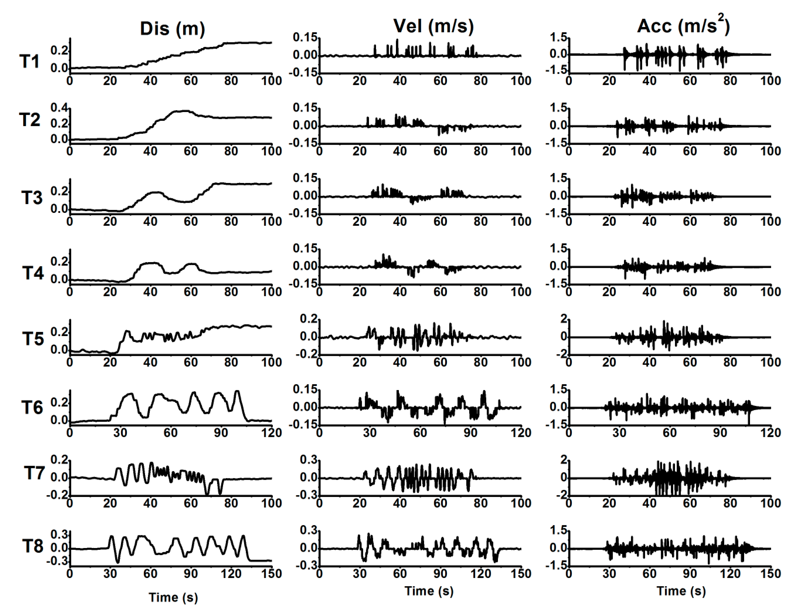
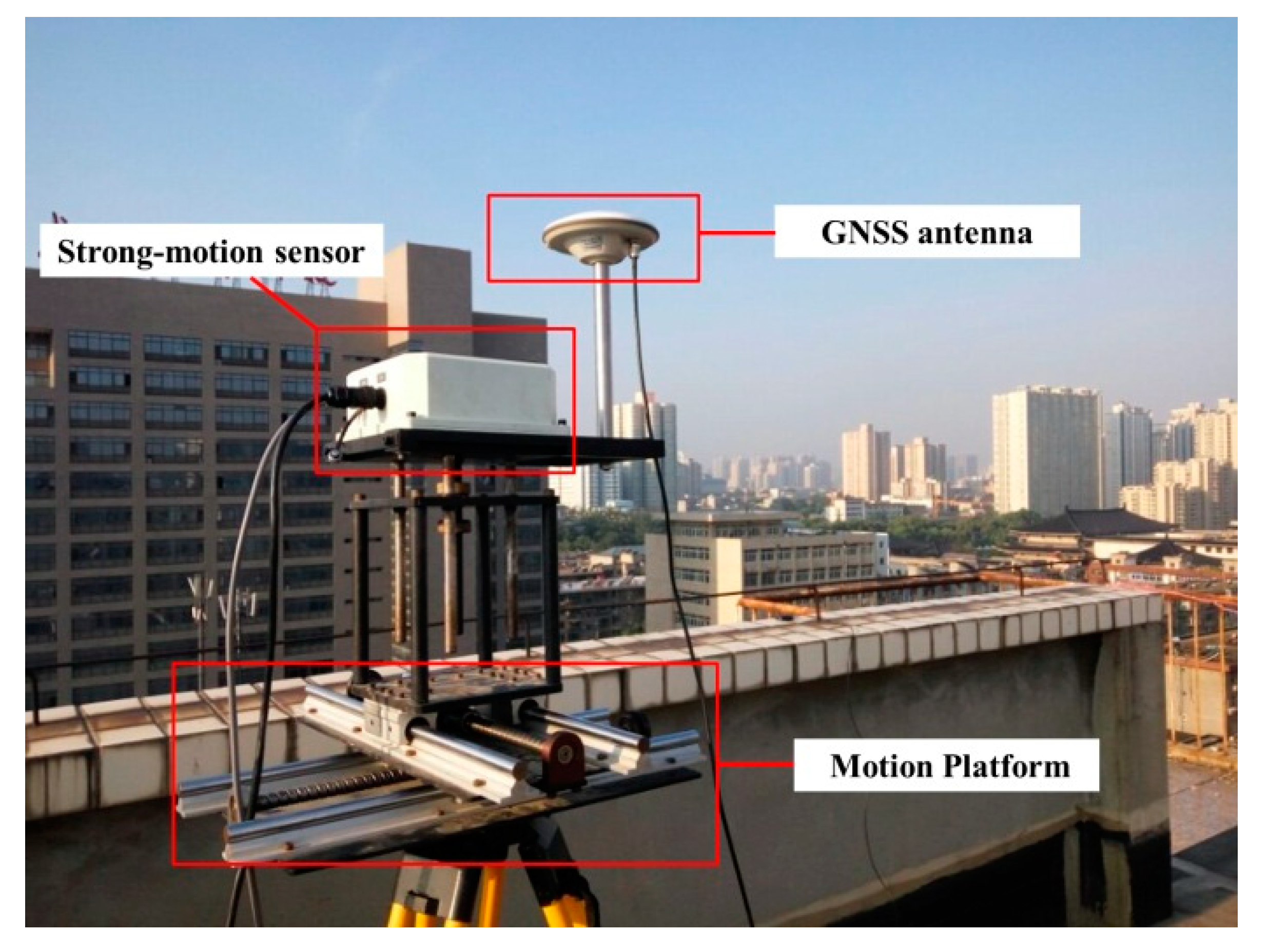
3.1. GPS and SM Data Test

Figure 5 shows the GPS and SM experimental platform, composed of a dynamic GPS antenna (Type: JAV_RINGANT_G3T NONE), a low-cost MEMS-type accelerometer [27], and real-time processing facilities. The experiment was carried out in December 2012; the sample rates were 50 Hz and 100 Hz for the single-frequency GPS and SM sensor, respectively. Real permanent displacement was provided by the Vernier calipers and the high-frequency camera to the front of the rig, and it was measured with a precision of better than 5 mm. Data processing used a high-frequency GPS and SM integration solution package developed by our research group.
Figure 6 shows the displacement sequence that was used for the test. We simulated eight events (T1 to T8) by moving the platform from one side to the other. The reference displacements were recorded by a set of Vernier calipers fixed on the table. For each experiment, we initially kept the rig static at the start point for about 5 min; then, we slid the combined instruments from the start point to the end point, for over about 1 min; next, the rig was kept static at the end point for about 5 min; finally, the rig was returned to the start point for the next experiment. For the eighth experiment, it was not returned to the start point, as this was the end of the experiment. Owing to the design of the platform, movement was performed only in one direction along the rail.
Figure 7 compares the displacement, velocity, and acceleration between GPS and SM individually and in combination for the first test. It can be concluded that the single-frequency GPS velocity estimation, which is based on broadcast ephemeris, can recover high-precision low-frequency displacement information; however, the velocity and acceleration are seriously distorted because of high-frequency noise pollution. In comparison, the SM-based acceleration has a much higher signal-to-noise ratio; however, the baseline-shift-corrected velocity and displacement show larger offsets than those for the GPS, while for the combination of GPS and SM measurements, both velocity and displacement are recovered in addition to the combined displacement, which is recovered with much less noise than the GNSS single system.
Figure 8 shows the power spectral densities (PSD) of the displacements obtained using different sensors; the top represents no motion, and the bottom represents the displacement motion. The GPS and SM combined system complements the advantages of each other, resulting in much smaller noise and much higher frequency than the GPS, and the removal of the baseline shift error in the SM.
Figure 9 shows the displacement, velocity, and acceleration outputs of the integration system, conforming that it accurately corrects the initial baseline shift of each system. Hence, the combined system effectively constrains the instantaneous complex baseline shift during an earthquake allowing high-precision broadband information to be retrieved in real-time.
Table 1 presents the final displacement and velocity biases compared to the references and their standard deviation statistics for all eight tests; all STDs are smaller than the thresholds. From these data, the accuracy of the displacement is 1–2   cm and the velocity is about 1   mm /s for the GPS and SM combined system.

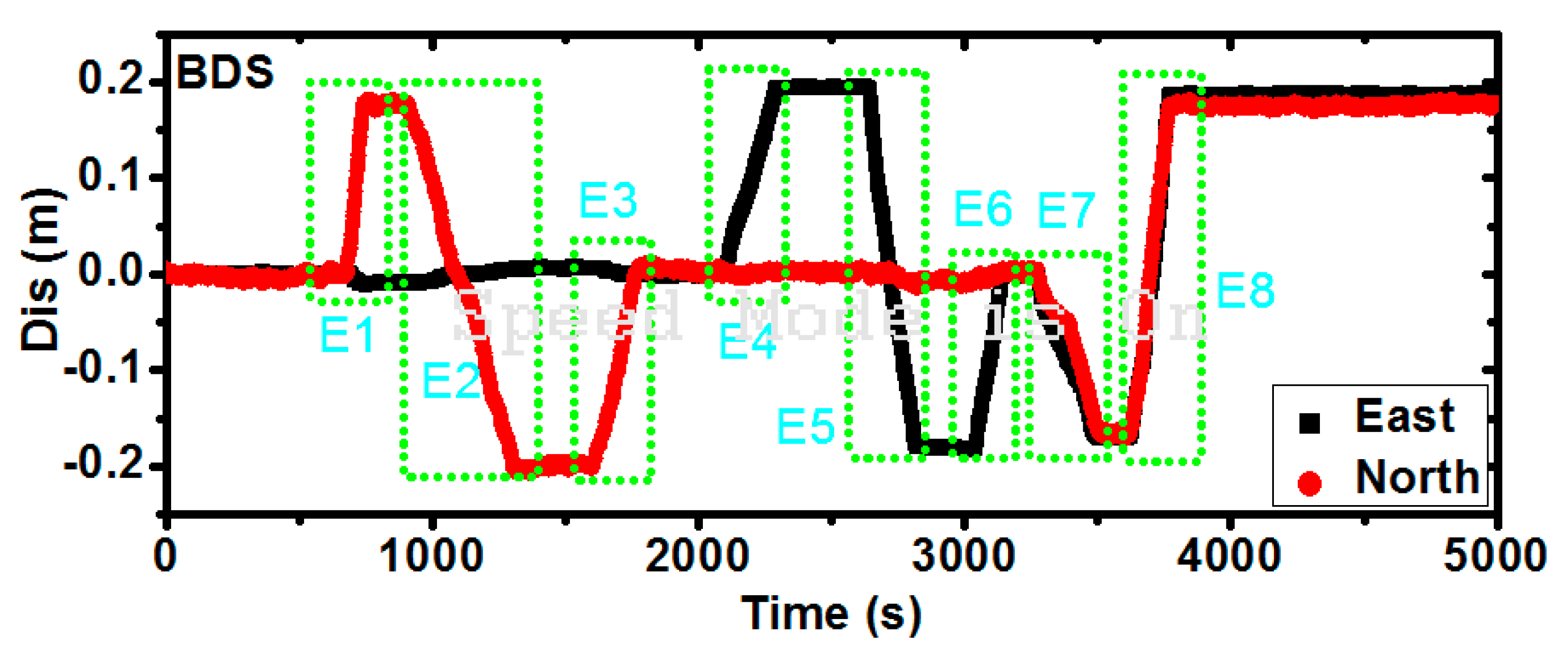
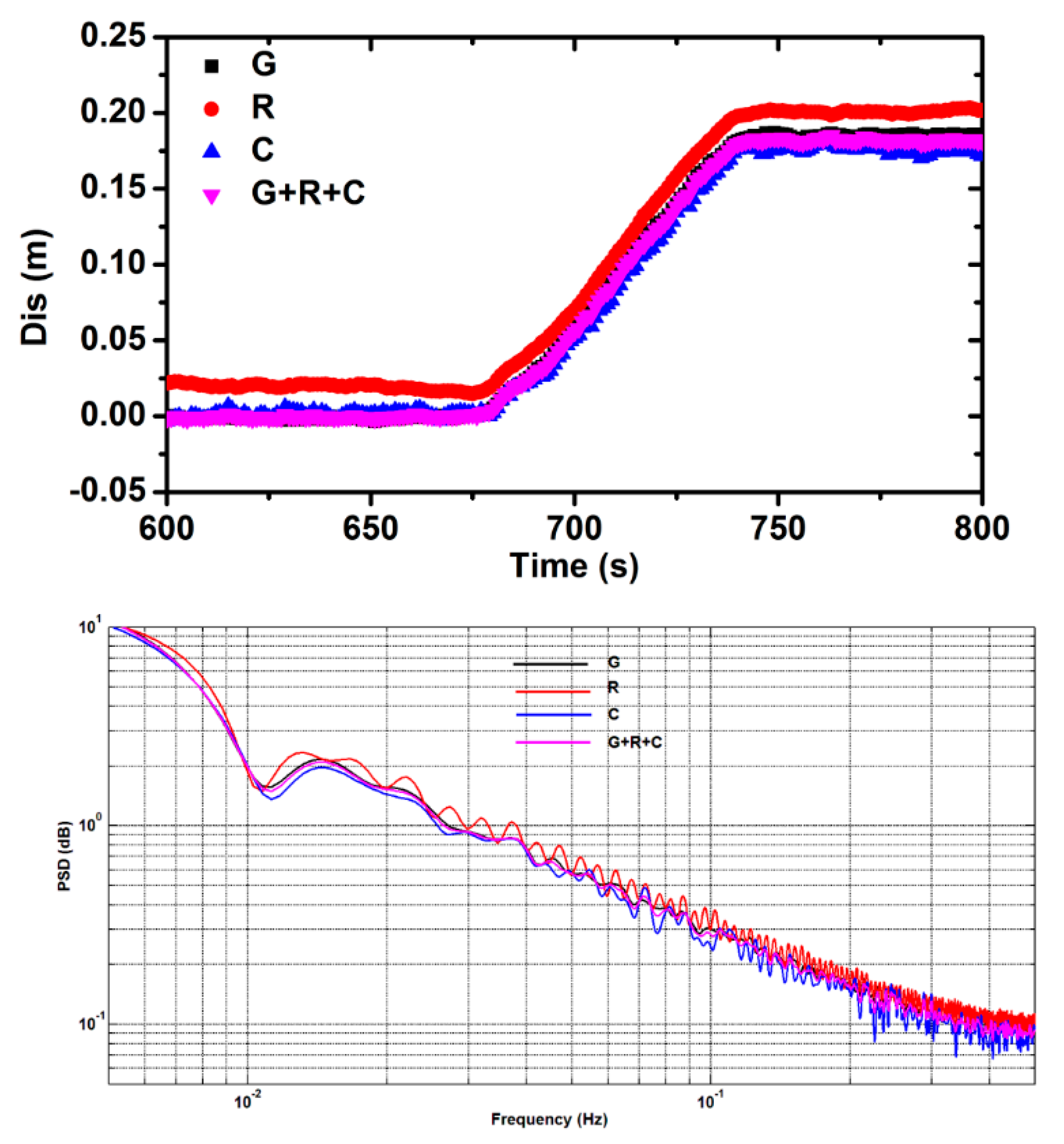
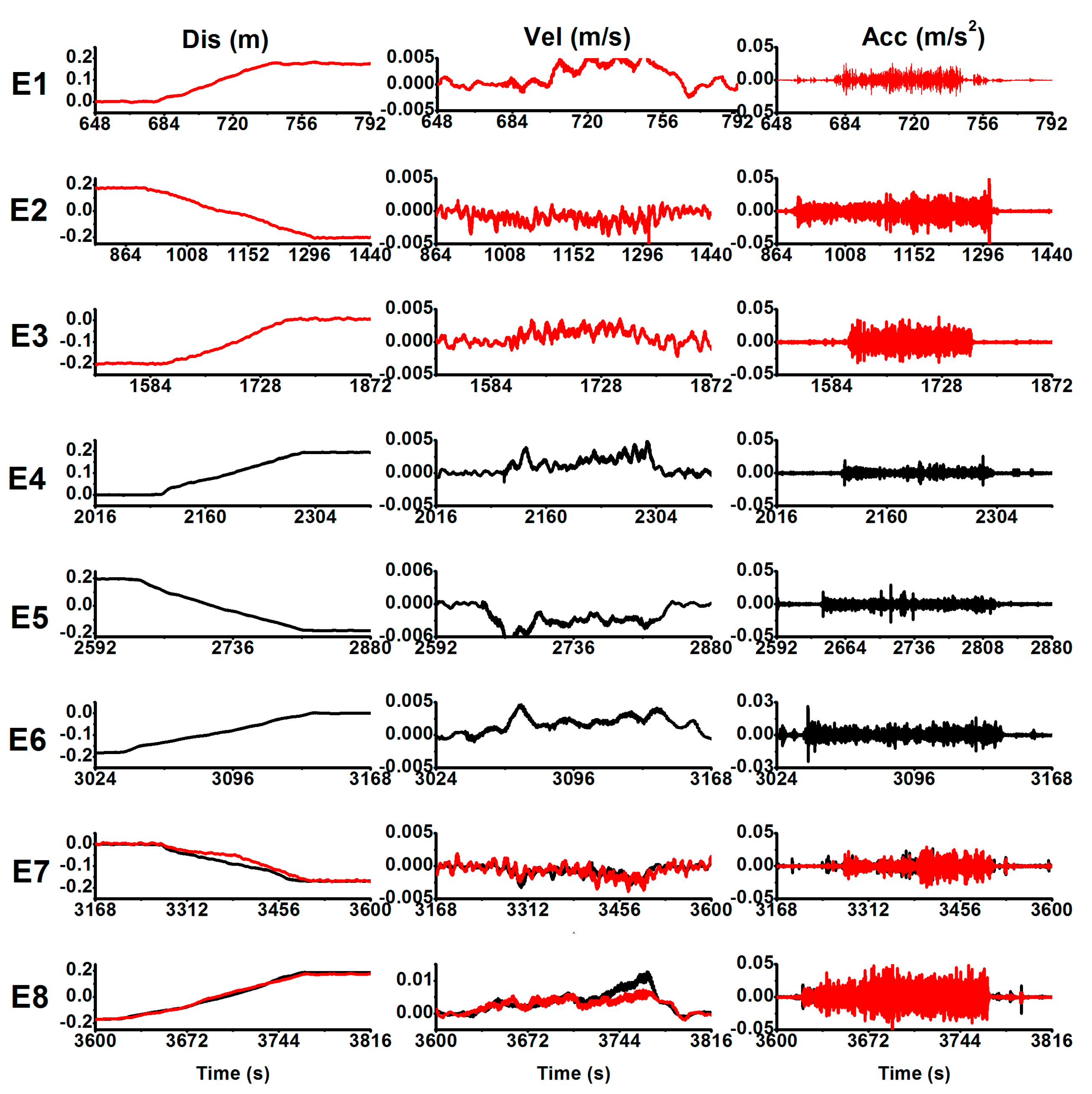
3.2. BDS and SM Data Test

BDS is a new GNSS system that is operated by China. Currently, it can provide positioning, navigation, and timing services in the Asia-Pacific region, and will expand to provide global coverage in 2020. We tested the performance of the integration of the BDS and SM system. Figure 10 shows another test platform used in the experiment performed in 2016 August in Xi’an, China. The platform, which can slide along a table, includes a dynamic GNSS antenna that can track BDS, GPS, and GLONASS signals (Type: UR380, Antenna: HX-GG486A), and a low-cost MEMS-type accelerometer [27]. The sampling rate was 1 Hz for GNSS and 100 Hz for the accelerometer. The maximum sliding distance of the platform is restricted to about 0.5 m. All data were processed in a simulated real-time mode. Here, we only analysed BDS and SM data.
Figure 11 shows the movement sequence applied to the BDS and SM integration experiment. We simulated eight earthquake events (E1–E8) by moving the platform from one side to the other. As for the previous experiment, reference displacements were recorded by a set of Vernier calipers fixed on the table. For each experiment, we kept the rig static at the start point for several minutes at first; then, we slid the combined instruments from the start point to the endpoint over about 1 or 2 min; and finally, the rig was kept static at the endpoint for several minutes, before starting the next experiment. We carried out eight experiments in the horizontal component: three in a north–south direction, three in an east–west direction, and two in a northeast–southwest direction.
As shown in previous studies, the performance of multi-GNSS systems is better than that of the single GNSS system [28,29,30,31,32]. Figure 12 shows a comparison of displacements and PSD for different GNSS systems for the first experiment. It can be seen that the precision of the GLONASS system was the worst because of fewer observed satellites. The BDS and GPS system nearly show the same accuracy, and their combination results are more stable. The PSD results reflect that BDS has much larger noise than GPS, and that the GLONASS has a small offset; the combination of multi-GNSS systems represents the average of each single system.
In Figure 13, the results of combining BDS and SM data for all eight experiments are illustrated. As expected, when the baseline shifts of the accelerations are corrected by the combined system, the high-resolution acceleration can help constrain the combination solution. Thus, high-precision and broadband deformation information (displacement, velocity, and acceleration) are recovered in real time.
Table 2 summarises the mean bias and STD between the recovered and references values. The RMS is generally less than 2 mm for velocity, and better than 2 cm for displacement.

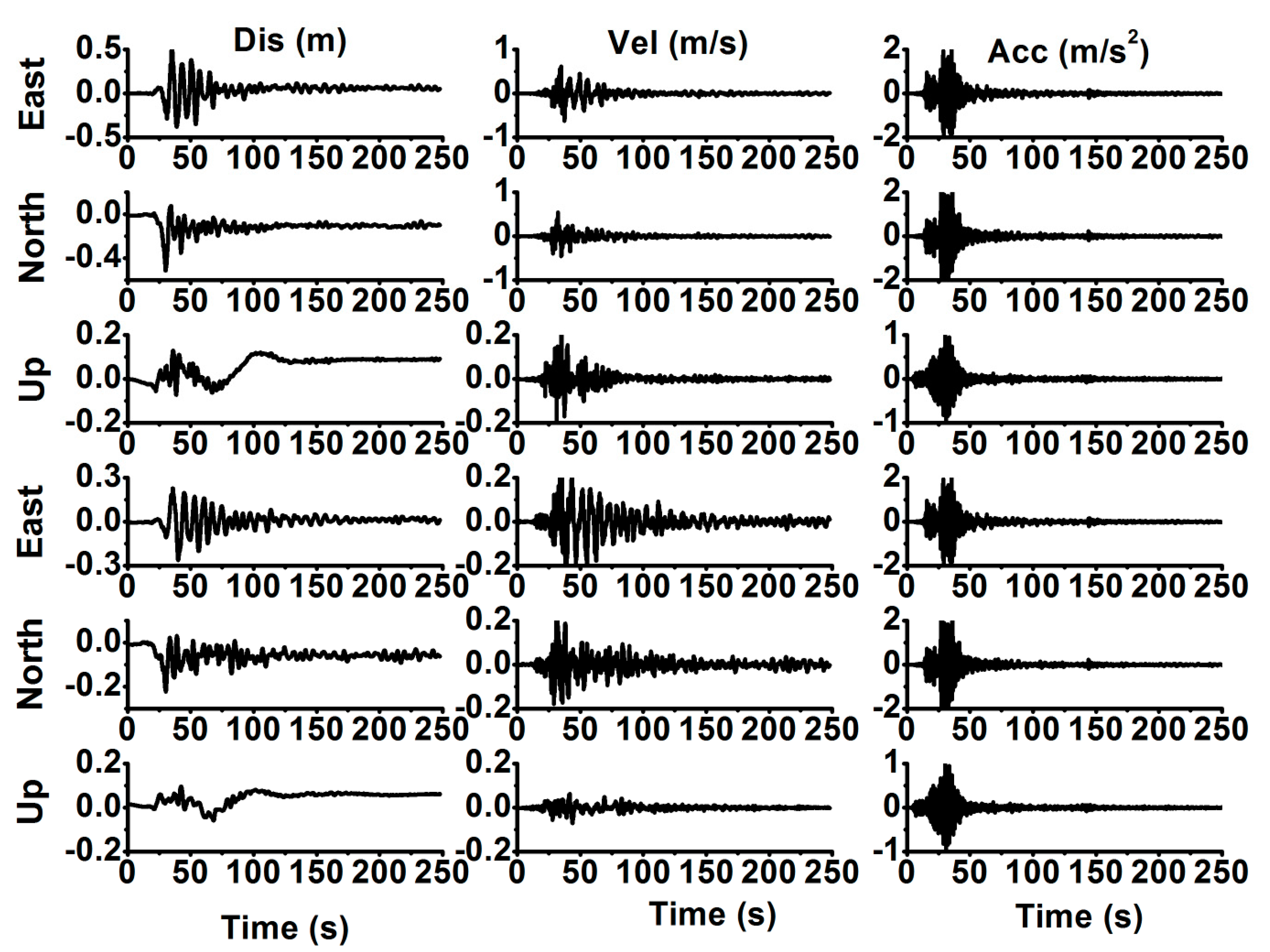
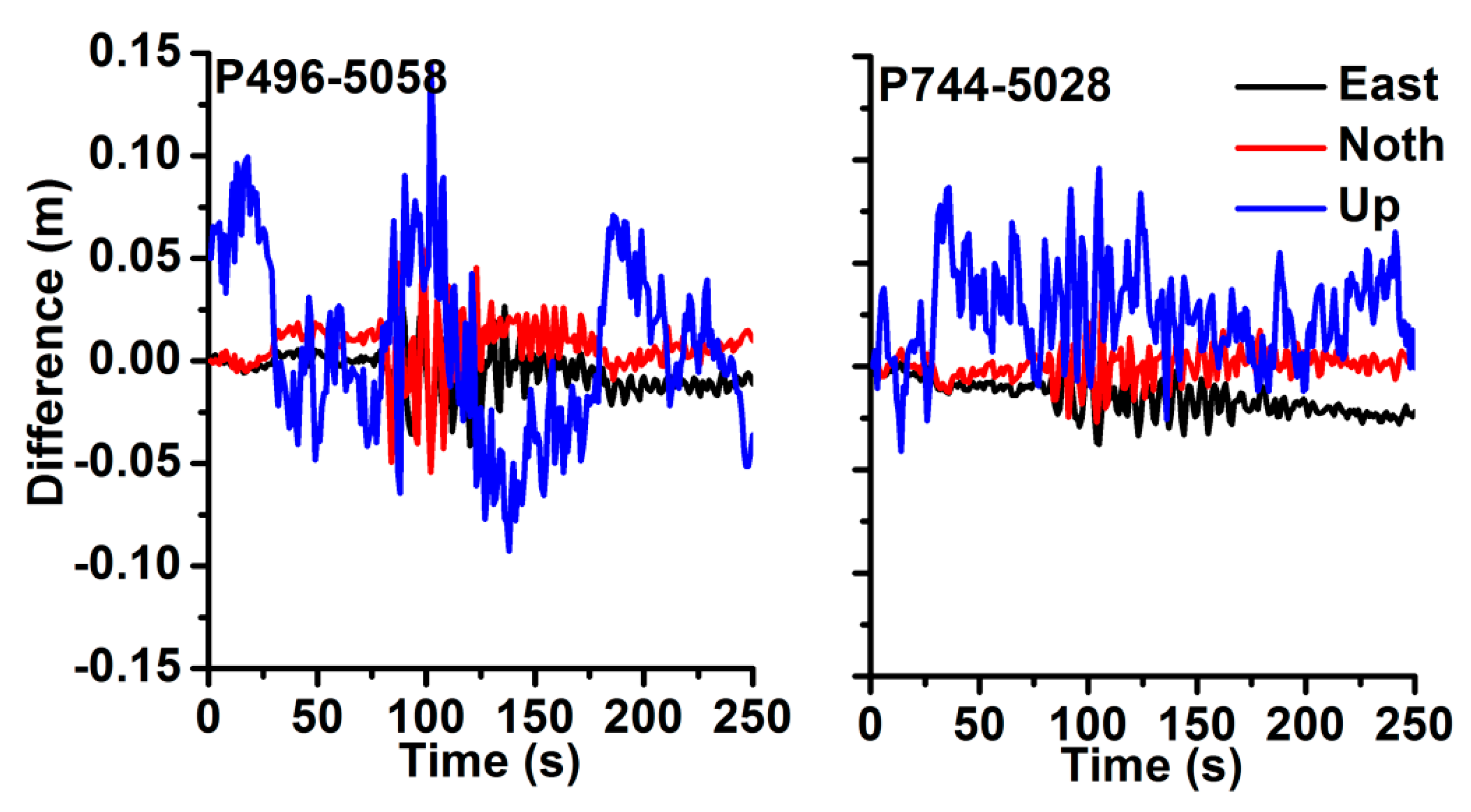
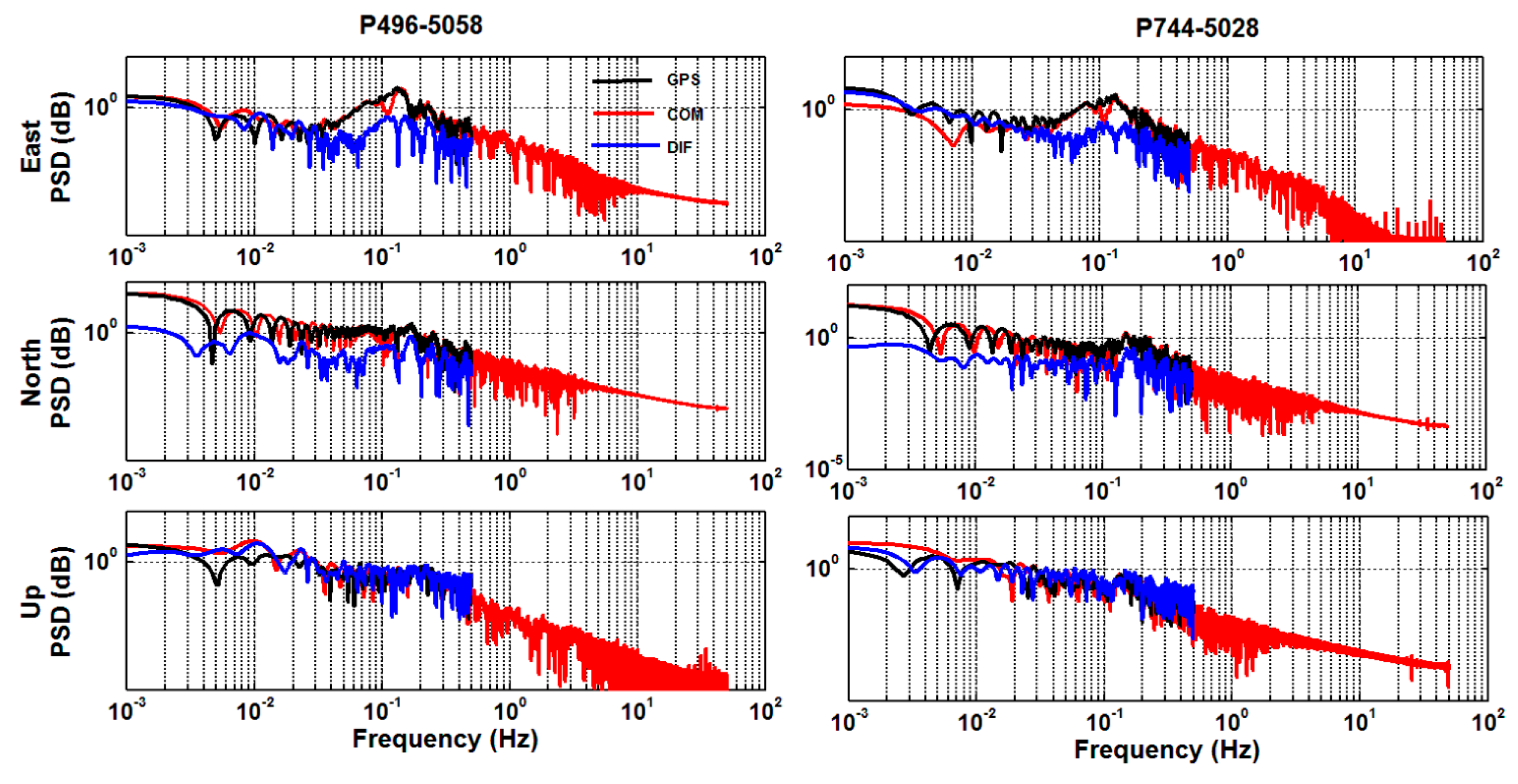
3.3. Baja Earthquake Data Test

After validation using two experimental datasets, co-located GPS and seismic data collected during the E1 Mayor-Cucapah earthquake (Mw, 7.2, 4 April 2010, 22:40:42 UTC) were also analysed. Two pairs of co-located GPS and SM seismometers were selected and processed. The GPS station P496, which is located 74 km from the earthquake epicentre, is nearly co-located with the seismic station 5058 of the Southern California Seismic Network (SCSN), within a distance of about 140 m. GPS station P744 located 80 km from the epicentre is about 275 m away from the nearest seismic station, 5028 in SCSN. The accelerometer data are 200 Hz, and the GPS data were recorded at 5 Hz.
Figure 14 shows the acceleration, velocity, and displacement information of the combined system in the east, north, and vertical components. The velocity sequence clearly reflects the waveform information, and the velocity fluctuates about the zero line after the earthquake. In the displacement sequence, the displacement fluctuates on the permanent displacement line.
In addition, the difference between GPS and the combined solution (by GPS and SM sensors) are shown in Figure 15. For the displacement, the residuals from the GPS and the integration method are nearly at the same level, the largest difference between the GPS and the combined solution is about 5 cm and most of them are smaller than 2 cm in the horizontal component. Additionally, it is much worse in the vertical component, the reasons may be owing to the GPS atmosphere error and SM baseline errors are not precisely corrected.
Table 3 shows the statistical results for these datasets. The reference displacement is provided by the GPS precise point positioning post solutions, with a precision of better than 5 mm. For the permanent displacement, which is calculated from the GPS post solutions, the mean difference in the horizontal components is 2–3 cm, and the average difference in the vertical components is about 4 cm. Such levels of displacement precision are much better than those of an individual SM seismometer, which has a displacement precision of the order of decimeters. Furthermore, the combined system can recover acceleration and velocity information, which the single GPS system cannot accurately provide. The vertical component of the GPS signal is subject to greater dithering than the horizontal components because the atmosphere error is difficult to process accurately in GPS epoch-differenced data; thus, the precision of the vertical displacement is worse than that of the horizontal components. These GPS errors will be included in the output of the combined system.
Meanwhile, the corresponding PSD are shows in Figure 16, we can see the GPS with much larger noise and narrower band than the combined results. Thus, the combined sensors best complement the advantages of GPS’s high precision and strong-motion’s high frequency.

4. Discussion

GNSS velocity estimation has significant potential benefits as it can be operated with a single station in real-time, and it does not need initialization. Previous studies have shown that 5 Hz GPS data can be used to recover a significant part of PGV values for large earthquakes [33].
For the application of velocity estimation, attention to details is important. As velocity estimation uses broadcast satellite ephemeris and epoch-differences, uncorrected atmosphere errors and ephemeris residuals will lead to shifts in estimated velocity. In this study, we treated these shifts as a linear model; the final precision may not be as high as with a linear correction, but linear corrections are, themselves, limited because they only work for short periods. In a future study, we plan to estimate GNSS shift as unknown parameters. In addition, for the epoch-difference solution, we plan to use the broadcast ephemeris record for the entire event period to avoid possible jumps in the results caused by discontinuities of adjacent ephemeris records.
Using only one kind of sensor has its limitations; the cooperation of different sensors can complement the advantages of each and it can, therefore, provide more reliable and robust information. The integration of multi-GNSS and SM is an interesting area of development for further research.
In this study, we proposed a combination approach by using single-frequency GNSS and low-cost SM observations. However, some of the validation data were not collected from the real single-frequency and/or low-cost sensors; thus, additional datasets are needed for further validation. Our results consider the complementary advantages of each sensor; however, inconsistencies between the two datasets may also depend on the frequency of the excitation, the direction of the excitation signal, and the distance from the excitation source; these need to be analysed in the future [34]. The analysis of noise in GNSS and SM measurements will also represent the focus of future work.
For real-time earthquake monitoring, the trigger mechanism is the most important. As the acceleration variation in SM data is more sensitive than that in GNSS data, we used the energy change from SM to detect the start of the combined system. When an event is detected, we required only a short period of pre-event data for the initialization; thus, when continuous events are detected, this combined system will not work. Furthermore, energy change not induced by earthquakes has no effect on the combined solution, which is processed by each collocated station; stations without influence are used for deformation monitoring, which is not limited to earthquakes.
The data solution of the combined system is based on the detection of an event. As the GNSS’ linear shift by epoch difference is also changing, the data solution is only effective for a short period; thus, it cannot be used for slow deformation hazards.

5. Conclusions

In this study, we developed a high-precision, full-frequency, and real-time earthquake monitoring system based on the integration of single-frequency GNSS and low-cost SM observations. The integrated system makes full use of the high-sensitivity of SM data to quickly and accurately determine the vibration window for the initial baseline shift correction before the earthquake and quality control after an earthquake. Additionally, it uses high-precision displacement recovered from the GNSS epoch-differenced velocity estimation to effectively constrain the SM low-frequency baseline shift. Hence, the integrated system can determine high-precision and full-frequency vibration information in real-time for the application of earthquake monitoring and early warning. Single-frequency GNSS and simple SM sensors are low cost; the acquisition of satellite broadcast ephemeris and observation data is straightforward in real-time; the data processing module can be embedded in the integrated instruments, enabling automatic operation for individual stations or single machines. Consequently, we believe that a real-time earthquake monitoring system based on this approach will be widely used in the future.

Author Contributions

R.T. and P.Z. conceived and designed the experiments; R.T. and R.Z. performed the experiments, analysed the data, and prepared the manuscript; and R.Z., J.L., and X.L. contributed to the discussions and revisions.

Acknowledgments

The work was partly supported by the program of National Key Research and Development Plan of China (Grant No. 2016YFB0501804), National Natural Science Foundation of China (Grant Nos. 41504006, 41674034) and Chinese Academy of Sciences (CAS) programs of ‘Pioneer Hundred Talents’ (Grant No. Y620YC1701), Light of the west joint scholar’ (Grant No. Y507YR1203), and ‘The Frontier Science Research Project’ (Grant No. QYZDB-SSW-DQC028).

Conflicts of Interest

The authors declare no conflict of interest.

References

  1. Colosimo, G.; Crespi, M.; Mazzoni, A. Real-time GPS seismology with a stand-alone receiver: A preliminary feasibility demonstration. J. Geophys. Res. 2011, 116, B11302. [Google Scholar] [CrossRef]
  2. Meng, X. From Structural Health Monitoring to Geo-Hazard Early Warning: An Integrated Approach Using GNSS Positioning Technology. In Earth Observation of Global Changes (EOGC); Springer: Berlin/Heidelberg, Germany, 2013; pp. 285–293. [Google Scholar]
  3. Bellone, T.; Dabove, P.; Manzino, A.M.; Taglioretti, C. Real-time monitoring for fast deformations using GNSS low-cost receivers. Geomat. Nat. Hazards Risk 2016, 7, 458–470. [Google Scholar] [CrossRef]
  4. Dabove, P.; Manzino, A. Kalman Filter as Tool for the Real-time Detection of Fast Displacements by the Use of Low-cost GPS Receivers. In Proceedings of the 2nd International Conference on Geographical Information Systems Theory, Applications and Management, Rome, Italy, 26–27 April 2016; pp. 15–23, ISBN 978-989-758-188-5. [Google Scholar] [CrossRef]
  5. Li, M.; Li, W.; Fang, R.; Shi, C.; Zhao, Q. Real-time high-precision earthquake monitoring using single-frequency GPS receivers. GPS Solut. 2015, 19, 27–35. [Google Scholar] [CrossRef]
  6. Elo’segui, P.; Davis, J.L.; Oberlander, D.; Baena, R.; Ekström, G. Accuracy of high-rate GPS for seismology. Geophys. Res. Lett. 2006, 33, L11308. [Google Scholar] [CrossRef]
  7. Genrich, J.F.; Bock, Y. Instantaneous geodetic positioning with 10–50 Hz GPS measurements: Noise characteristics and implications for monitoring networks. J. Geophys. Res. 2006, 111, B03403. [Google Scholar] [CrossRef]
  8. Larson, K.M.; Bilich, A.; Axelrad, P. Improving the precision of high-rate GPS. J. Geophys. Res. 2007, 112, B05422. [Google Scholar] [CrossRef]
  9. Iwan, W.; Moser, M.; Peng, C. Some observations on strong-motion earthquake measurement using a digital acceleration. Bull. Seismol. Soc. Am. 1985, 75, 1225–1246. [Google Scholar]
  10. Boore, D.M. Effect of baseline corrections on displacement and response spectra for several recordings of the 1999 Chi-Chi, Taiwan, earthquake. Bull. Seismol. Soc. Am. 2001, 91, 1199–1211. [Google Scholar] [CrossRef]
  11. Zhu, L. Recovering permanent displacements from seismic records of the June 9, 1994 Bolivia deep earthquake. Geophys. Res. Lett. 2003, 30, 1740. [Google Scholar] [CrossRef]
  12. Graizer, V. Tilts in strong ground motion. Bull. Seismol. Soc. Am. 2006, 96, 2090–2106. [Google Scholar] [CrossRef]
  13. Wu, Y.; Wu, C. Approximate recovery of coseismic deformation from Taiwan strong-motion records. J. Seismol. 2007, 11, 159–170. [Google Scholar] [CrossRef]
  14. Wang, R.; Schurr, B.; Milkereit, C.; Shao, Z.; Jin, M. An improved automatic scheme for empirical baseline correction of digital strong-motion records. Bull. Seismol. Soc. Am. 2011, 101, 2029–2044. [Google Scholar] [CrossRef]
  15. Bock, Y.; Melgar, D.; Crowell, B.W. Real-time strong-motion broadband displacements from collocated GPS and accelerometers. Bull. Seismol. Soc. Am. 2011, 101, 2904–2925. [Google Scholar] [CrossRef]
  16. Tu, R.; Wang, R.; Ge, M.; Walter, T.R.; Ramatschi, M.; Milkereit, C.; Bindi, D.; Dahm, T. Cost effective monitoring of ground motion related to earthquakes, landslides or volcanic activities by joint use of a single-frequency GPS and a MEMS accelerometer. Geophys. Res. Lett. 2013, 40, 3825–3829. [Google Scholar] [CrossRef]
  17. Tu, R.; Ge, M.; Wang, R.; Walter, T.R. A new algorithm for tight integration of real-time GPS and strong-motion records, demonstrated on simulated, experimental, and real seismic data. J. Seismol. 2014, 18, 151–161. [Google Scholar] [CrossRef]
  18. Tu, R.; Wang, R.; Walter, T.R.; Diao, F.Q. Adaptive recognition and correction of baseline shifts from collocated GPS and accelerometer using two phases Kalman filter. Adv. Space Res. 2014, 54, 1924–1932. [Google Scholar] [CrossRef]
  19. Tu, R.; Zhang, Q.; Wang, L.; Liu, Z.K.; Huang, G.W. An improved method for tight integration of GPS and strong-motion records: Complementary advantages. Adv. Space Res. 2015, 56, 2335–2344. [Google Scholar] [CrossRef]
  20. Tu, R.; Liu, J.H.; Lu, C.X.; Zhang, R.; Zhang, P.F.; Lu, X.C. Cooperating the BDS, GPS, GLONASS and strong-motion observations for real-time deformation monitoring. Geophys. J. Int. 2017, 209, 1408–1417. [Google Scholar] [CrossRef]
  21. Geng, J.; Bock, Y.; Melgar, D.; Crowell, B.W.; Haase, S. A new seismogeodetic approach applied to GPS and accelerometer observations of the 2012 Brawley seismic swarm: Implications for earthquake early warning. Geochem. Geophys. Geosyst. 2013, 14, 2124–2142. [Google Scholar] [CrossRef] [Green Version]
  22. Li, X.; Ge, M.; Zhang, Y.; Wang, R.; Klotz, J.; Wicket, J. High-rate coseismic displacements from tightly-integrated processing of raw GPS and accelerometer data. Geophys. J. Int. 2013, 195, 612–624. [Google Scholar] [CrossRef]
  23. Wang, R.; Parolai, S.; Ge, M.; Jin, M.; Walter, T.R.; Zschau, J. The 2011 Mw 9.0 Tohoku-Oki earthquake: Comparison of GPS and Strong-motion. Bull. Seismol. Soc. Am. 2012. [Google Scholar] [CrossRef]
  24. Geng, J.; Bock, Y.; Melgar, D.; Crowell, B.; Haase, J. A new seismogeodetic approach applied to GPS and accelerometer observations of the 2012 Brawley seismic swarm: Implications for earthquake early warning. Geochem. Geophys. Geosyst. 2013, 14, 2124–2142. [Google Scholar] [CrossRef] [Green Version]
  25. Geng, J.; Melgar, D.; Bock, Y.; Pantoli, E.; Restrepo, J. Recovering coseismic point ground tilts from collocated high-rate GPS and accelerometers. Geophys. Res. Lett. 2013, 40, 5095–5100. [Google Scholar] [CrossRef] [Green Version]
  26. Saunders, J.; Goldberg, E.; Haase, J.; Bock, Y.; Offield, D.; Melgar, D.; Restrepo, J.; Fleischman, R.; Nema, A.; Geng, J.; et al. Seismogeodesy Using GPS and Low-Cost MEMS Accelerometers:Perspectives for Earthquake Early Warning and Rapid Response. Bull. Seismol. Soc. Am. 2016, 106, 2469–2489. [Google Scholar] [CrossRef]
  27. Fleming, K.; Picozzi, M.; Milkereit, C.; Kuehnlenz, F.; Lichtblau, B.; Fischer, J.; Zulfikar, C.; Ozel, O. The SAFER and EDIM Working Groups. The Self-Organising Seismic Early Warning Information System (SOSEWIN). Seismol. Res. Lett. 2009, 80, 755–771. [Google Scholar] [CrossRef]
  28. Msaewe, H.; Hancock, C.; Psimoulis, P.; Roberts, G.; Bonenberg, L. Monitoring Dynamic Deflections at Towers of Severn Suspension Bridge in the UK Using GNSS Technique. In Proceedings of the ISGNSS, Hong Kong, China, 10–13 December 2017. [Google Scholar]
  29. Roberts, G.; Tang, X.; He, X. Accuracy analysis of GPS/BDS relative positioning using zero-baseline measurements. J. Glob. Position. Syst. 2018, 16, 7. [Google Scholar] [CrossRef] [Green Version]
  30. Psimoulis, P.; Pytharouli, S.; Karambalis, D.; Stiros, S. Potential of GPS to measure frequencies of oscillation of engineering structures. J. Sound Vib. 2008, 318, 606–623. [Google Scholar] [CrossRef]
  31. Moschas, F.; Stiros, S. Dynamic Deflections of a Stiff Footbridge Using 100-Hz GNSS and Accelerometer Data. J. Surv. Eng. 2015, 141, 04015003. [Google Scholar] [CrossRef]
  32. Häberling, S.; Rothacher, M.; Zhang, Y.; Clinton, J.; Geiger, A. Assessment of high-rate GPS using a single-axis shake table. J. Geod. 2015, 89, 697–709. [Google Scholar] [CrossRef]
  33. Michel, C.; Kelevitz, K.; Houlié, N.; Edwards, B.; Psimoulis, P.; Su, Z.; Clinton, J.; Giardini, D. The Potential of High-Rate GPS for Strong Ground Motion Assessment. Bull. Seismol. Soc. Am. 2017, 107, 1849–1859. [Google Scholar] [CrossRef]
  34. Psimoulis, P.; Houlié, N.; Meindl, M.; Rothacher, M. Consistency of GPS and strong-motion records: Case study of Mw9.0 Tohoku-Oki 2011 earthquake. Smart Struct. Syst. 2015. [Google Scholar] [CrossRef]
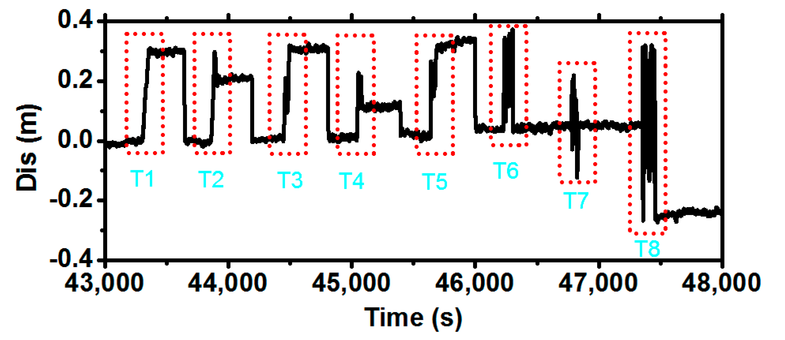
Figure 1. Comparison of average energies for GNSS (bottom) and SM (top) detectors.
Remotesensing 10 00886 g001
Figure 2. Correction of initial baseline shift for GNSS (top) and strong-motion (bottom). The black line represents raw values; the red line, estimated corrections; and the blue line, corrected values.
Remotesensing 10 00886 g002
Figure 3. Quality evaluation of the displacement and velocity after an earthquake. The upper graph shows the displacement, which is stable around a fixed offset; the lower graph shows the velocity, which is stable around 0 m/s.
Remotesensing 10 00886 g003
Figure 4. Real-time integration system of GNSS and SM observations. ‘RT’ indicates real-time, ‘Dis, Vel, and Acc’ represent displacement, velocity and acceleration, respectively, ‘obs’ represents observation, and ‘eph’ represents ephemeris.
Remotesensing 10 00886 g004
Figure 5. Experimental platform (left) and processing facilities (right) of the combined system GPS and SM system.
Remotesensing 10 00886 g005
Figure 6. Movement sequence of the GPS and SM experiments. The graph covers the time for eight tests (T1–T8), each indicated by a dashed red rectangle.
Remotesensing 10 00886 g006
Figure 7. Comparisons of displacement, velocity, and acceleration for the GPS (left); SM (middle); and combined system (COM) (right).
Remotesensing 10 00886 g007
Figure 8. Comparison of the PSD for the displacements of the first experiment by different sensors. Black, blue and red lines represent the GPS, SM, and the combined system, respectively, the (top) represents no motion and (bottom) represents displacement motion.
Remotesensing 10 00886 g008
Figure 9. Displacement (left); velocity (middle); and acceleration (right) output of the integration system for the GPS and SM data. Note that vertical scales vary between the tests.
Remotesensing 10 00886 g009
Figure 10. Experimental equipment used to test the integration of BDS and SM data. Hardware consists of a GNSS sensor, an SM sensor, and a tracked platform.
Remotesensing 10 00886 g010
Figure 11. Movement sequence of eight BDS and SM experiments. Each green dotted rectangle represents one test.
Remotesensing 10 00886 g011
Figure 12. Comparison of displacements (top) and PSD (bottom) for different GNSS systems. Black, blue, red, and pink lines represent the GPS, GLONASS, BDS, and their combinations, respectively.
Remotesensing 10 00886 g012
Figure 13. Displacement (left); velocity (middle); and acceleration (right) output of the integration system for the BDS and SM data. Black curves indicate east–west displacement of the test bed, whereas the red curves indicate north–south motion.
Remotesensing 10 00886 g013
Figure 14. Displacement (left); velocity (middle); and acceleration (right) output of the integration system for the Baja earthquake data. The upper three plots represent pairs of ‘P496-5058’; the lower three plots represent pairs of ‘P744-5028’.
Remotesensing 10 00886 g014
Figure 15. Differences of displacement waveforms between GPS and combined solutions. The (left) represents pairs of ‘P496-5058’; the (right) represents pairs of ‘P744-5028’.
Remotesensing 10 00886 g015
Figure 16. PSD of displacement waveforms by different methods (‘‘COM” represents the GPS and SM combined results, ‘‘DIF” represents the difference between GPS and combined results). The (left) represents pairs of ‘P496-5058’; the (right) represents pairs of ‘P744-5028’.
Remotesensing 10 00886 g016
Table 1. Quality statistics results for the GPS and SM data. D indicates the displacement (m) and V indicates velocity (m/s).
TestD-BiasD-STDV-BiasV-STDTestD-BiasD-STDV-BiasV-STD
T1−0.0060.0021.3 × 10−40.001T50.0120.0031.2 × 10−40.001
T20.0110.0031.1 × 10−40.001T60.0080.002−1.0 × 10−40.001
T30.0130.003−1.1 × 10−40.001T70.0160.0031.4 × 10−40.001
T4−0.0140.0021.2 × 10−40.001T8−0.0130.0031.1 × 10−40.001
Table 2. Quality statistics for the BDS and SM data (D indicates displacement (m), V indicates velocity (m/s), and N and E represent the north and east components, respectively).
TestD-BiasD-STDV-BiasV-STDTestD-BiasD-STDV-BiasV-STD
E1(N)−0.0130.0021.3 × 10−40.001E4(E)−0.0140.0020.6 × 10−40.001
E2(N)0.0140.0021.0 × 10−40.001E5(E)0.0120.0031.1 × 10−40.001
E3(N)0.0130.0020.9 × 10−40.001E6(E)0.0130.0022.0 × 10−40.001
E7(E)0.0160.0031.0 × 10−40.001E7(N)0.0150.0021.1 × 10−40.001
E8(E)0.0130.003−0.9 × 10−40.001E8(N)0.0170.003−1.4 × 10−40.001
Table 3. Quality statistics for Baja earthquake data. D indicates displacement (m), V indicates velocity (m/s).
PairsComponentD-BiasD-STDV-BiasV-STD
P496-5058East0.0260.0031.4 × 10−40.002
North0.0110.003−1.2 × 10−40.002
Up0.0440.0051.0 × 10−40.001
P744-5028East0.0210.0021.3 × 10−40.002
North0.0180.0031.0 × 10−40.002
Up0.0360.004−0.9 × 10−40.001

