Article

An Enhanced Linear Spatio-Temporal Fusion Method for Blending Landsat and MODIS Data to Synthesize Landsat-Like Imagery

1
Institute of Surface-Earth System Science, Tianjin University, Tianjin 300072, China
2
National Marine Data and Information Service, Tianjin 300171, China
3
LREIS, Institute of Geographic Sciences and Natural Resources Research, University of the Chinese Academy of Sciences, Beijing 100101, China
*
Author to whom correspondence should be addressed.
Remote Sens. 2018, 10(6), 881; https://doi.org/10.3390/rs10060881
Submission received: 26 April 2018 / Revised: 31 May 2018 / Accepted: 5 June 2018 / Published: 5 June 2018
(This article belongs to the Special Issue Multisensor Data Fusion in Remote Sensing)

Abstract

:
Landsat and MODIS data have been widely utilized in many remote sensing applications, however, the trade-off between the spatial resolution and temporal frequency has limited their capacities in monitoring detailed spatio-temporal dynamics. Spatio-temporal fusion methods based on a linear model that considers the differences between fine- and coarse-spatial-resolution images as linear can effectively solve this trade-off problem, yet the existing linear fusion methods either regard the coefficients of the linear model as constants or have adopted regression methods to calculate the coefficients, both of which may introduce some errors in the fusion process. In this paper, we proposed an enhanced linear spatio-temporal fusion method (ELSTFM) to improve the data fusion accuracy. In the ELSTFM, it is not necessary to calculate the slope of the linear model, and the intercept, which can be deemed as the residual caused by systematic biases, is calculated based on spectral unmixing theory. Additionally, spectrally similar pixels in a given fine-spatial-resolution pixel’s neighborhood and their corresponding weights were used in the proposed method to mitigate block effects. Landsat-7/ETM+ and 8-day composite MODIS reflectance data covering two study sites with heterogeneous and homogenous landscapes were selected to validate the proposed method. Compared to three other typical spatio-temporal fusion methods visually and quantitatively, the predicted images obtained from ELSTFM could acquire better results for the two selected study sites. Furthermore, the resampling methods used to resample MODIS to the same spatial resolution of Landsat could slightly, but did not significantly influence the fusion accuracy, and the distributions of slopes of different bands for the two study sites could all be deemed as normal distributions with a mean value close to 1. The performance of ELSTFM depends on the accuracy of residual calculation at fine-resolution and large landscape changes may influence the fusion accuracy.

Graphical Abstract

1. Introduction

Landsat data at 30 m resolution have been widely applied for ecological system variation studies [1], environmental monitoring [2], and detailed land use and land cover mapping [3,4] because of their rich archives and free availability (more than four decades from the launch of Landsat-1 in 1972 to Landsat-8 with the OLI/TIRS imager launched on 11 February 2013). However, their 16-day revisit-cycles, even longer because of frequent cloud contamination and other inferior atmospheric conditions, limit their applications in dynamics monitoring. Leckie [5] found that for a given temporal coverage, the probability of obtaining Landsat images with less than 10% cloud cover could be as low as 10% for some regions in Canada. Furthermore, for tropical regions where cloud coverage is frequent, cloud contamination still limits the usages of Landsat data [6]. On the other hand, the moderate resolution imaging spectroradiometer (MODIS) images have also been widely employed for dynamics and process monitoring in global- or large-scale regions [7,8,9,10]. MODIS imagery has a daily revisit period, but its spatial resolution (from 250 m to 1 km) cannot perfectly meet the fine-scale environmental applications [11]. Additionally, although some new satellites can provide high spatial resolution data frequently, such as the Sentinel-2 series, which can provide data covering the same area every 10 days (5 days with two satellites together) with four bands at 10 m, six bands at 20 m, and three bands at 60 m spatial resolution, however, due to both cloud and shadow contamination, the temporal interval between two successive cloud-free images for specific areas may be more than several months [12]. Hence, up to now, a trade-off between spatial and temporal resolutions still exists in remote sensing instruments and one effective way to solve this trade-off problem is spatio-temporal fusion, which aims to blend images with fine spatial resolution but low frequency (such as Landsat data, referred to as fine-spatial-resolution images) and images with high temporal frequency but coarse spatial resolution (such as MODIS data, referred as coarse-spatial-resolution images) to synthesize data with high spatial resolution and temporal frequency.
Spatio-temporal fusion methods based on a linear model have been developed for many years, which deem the reflectance of fine- and coarse-spatial-resolution images as linear and the predicted reflectance can be directly obtained by adding the temporal changes to the observed fine-spatial-resolution images. Gao et al. [13] first proposed the spatial and temporal adaptive reflectance fusion model (STARFM) to synthesize the Landsat-like data by combining the MODIS and Landsat data. The theoretical basis of STARFM is that the reflectance of pixels acquired from homogeneous regions are comparable and consistent in fine- and coarse-spatial-resolution images. Then, the predicted synthetic values can be obtained by adding the changes derived from coarse-spatial-resolution pixels to the corresponding observed fine-spatial-resolution pixels. Additionally, to decrease the effects of mixed pixels and to enhance the fusion accuracy, neighboring spectrally similar pixels at fine-resolution are selected and a weighed sum algorithm using all similar pixels is used to calculate the final predicted reflectance. Though the STARFM can predict the fine-spatial-resolution pixels, the performance of STARFM for reflectance change areas and heterogeneous landscapes is not satisfactory, and therefore some improved methods derived from the STARFM method have been developed. Hilker et al. [14] presented a spatial and temporal adaptive algorithm for mapping reflectance change (STAARCH), which could enhance the fusion accuracy in land cover change regions by identifying highly detailed spatio-temporal patterns. Zhu et al. [11] introduced enhanced STARFM (ESTARFM), which could increase fusion accuracy in heterogeneous areas by introducing the conversion coefficient. The STARFM and its improved models have been widely used to support various applications such as leaf area index assimilation [15], urban heat island effect monitoring [16], land surface temperature generating [17], crop types and dynamics mapping [18,19,20], land cover classification [21], and land surface water mapping [22].
Recently, some new linear models have deemed the temporal changes between two coarse-spatial-resolution images as linear in a short period. The theoretical basis is that the coefficients for the linear equation formed using two coarse-spatial-resolution images at the reference and prediction dates can be directly applied to the fine-spatial-resolution images and then the unknown prediction at fine resolution can be acquired. Cheng et al. [23] presented the spatial and temporal nonlocal filter-based fusion model (STNLFFM). The coefficients of the linear equation of a given pair of coarse-spatial-resolution pixels can be acquired by using the least square method based on the neighboring pixels and the given pixels themselves. Then, the coefficients can be used for the observed fine-spatial-resolution image to acquire the prediction. To decrease the effects of heterogeneous landscapes, the STNLFFM uses the neighboring spectrally similar pixels to make a more accurate prediction. Similarly, Wang and Atkinson [12] proposed a linear model (hereafter referred to as Fit_FC) that contained three main steps: (1) regression model fitting was used to calculate the coefficients of linear model; (2) spatial filtering was used to deal with the blocky artifacts problem created in the first step; and (3) residual compensation was used to distribute the residuals generated in the first step.
Alternatively, the unmixing-based model is also a significant component in spatio-temporal fusion. Zurita-Milla et al. [24] used the unmixing-based method to blend TM and medium resolution imaging spectrometer (MERIS) data. Generally, the land-use databases on the study areas are necessary for the unmixing-based model, however, the land-use databases are not always available or have not been updated for specific regions, hence, some unmixing-based methods use unsupervised classification methods to generate classification maps. Based on land-use databases or classification maps, the abundances of all classes in a given coarse-spatial-resolution pixel and its neighboring pixels can be obtained. By using the least square method, the spectral values of endmembers (i.e., fine-spatial-resolution pixels) located in the central coarse-spatial-resolution pixels can be calculated. Some improved unmixing-based methods have been proposed to enhance the fusion accuracy. Instead of unmixing the coarse-spatial-resolution pixels, Gevaert and Garcia-Haro [25] estimated the changes of endmembers by directly unmixing the changes of coarse-spatial-resolution pixels and Bayesian theory was used to constrain the estimation to avoid the outliers. Xie et al. [26] first used unmixing-based methods to downscale the two coarse-spatial-resolution images at the reference and prediction dates, and then based on the downscaled coarse-spatial-resolution images, the STARFM was employed to synthesize the fine-spatial-resolution image. Wu et al. [27] proposed the spatial temporal data fusion approach (STDFA), which regarded the temporal variation properties of pixels belonging to the identical class as unchanged. Then, Wu et al. [28] proposed an improved version of STDFA, which took the spatial-variability adjustment and sensor-difference adjustment into account. Zhu et al. [29] first used the “purest” coarse-spatial-resolution pixels to calculate the temporal changes of endmembers by using the unmixing method. Then, the errors from homogeneous and heterogeneous regions were considered separately and through the homogeneity index, these two types of errors were combined to modify the temporal changes obtained in the first step. Finally, the neighboring spectrally similar pixels were used to mitigate block effects. We refer to this method as FSDAF in this paper. By introducing the temporal changes modification, FSDAF could better predict the areas where land cover type changes between the reference and prediction dates. The unmixing-based methods have also been used in many applications such as NDVI series generating [30,31] and crop monitoring [32]. Additionally, some learning-based methods based on the mechanism of machine learning have nowadays been proposed including mainly sparse representation [33,34], extreme learning machine [35], and deep learning [36].
All of the above spatio-temporal fusion approaches can obtain accurate synthetic data, but some errors still inevitably exist in the fused process. Generally speaking, for the homogeneous fine- and coarse-spatial-resolution pixels at the same location, the relationship between them can be described using the linear model as:
M = a × L + b
where L and M refer to the fine- and coarse-spatial-resolution pixels (in this paper, they refer to Landsat and MODIS data, respectively) and a and b are two coefficients of the linear model. How to accurately predict these two coefficients is essential for the fusion methods based on the linear model. For STARFM and ESTARFM, coefficient a is considered to be equal to either 1 or a constant, however, the coefficients a and b may vary at different locations. Hence, the assumption of STARFM and ESTARFM may introduce some errors in fusion. On the other hand, similar to the ideas of some linear models [12,23], the coefficients a and b can be calculated by using the least square method. Generally, the pixels obtained from coarse-spatial-resolution images at the reference and prediction dates in a moving window are usually used to get the coefficients of the central pixel. Even though the regression model can accurately predict the coefficients in some regions, some fitting errors inevitably exist in the data fitting process. Especially, when the differences of pixels used to calculate the coefficients in the moving window are relatively large, caused probably by the temporal changes of landscapes, the fitting coefficients may result in great errors between the fitting values and the actual values. Theoretically, the more coarse-spatial-resolution pixels are considered, the lower the fitting errors that will be generated.
Hence, we proposed an enhanced linear spatio-temporal fusion model (ELSTFM). The ELSTFM is based on the linear model, but it is not necessary to calculate coefficient a and coefficient b is acquired based on the unmixing-based theory (discussed in Section 2). There are two main advances of the ELSTFM: (1) the two coefficients a and b are not invariable and can be determined locally; and (2) the fitting process is not necessary, so the fitting errors can be partly depressed, meanwhile, the subjective window size setting in the fitting process also becomes an unnecessary step. Therefore, the ELSTFM can enhance the accuracy of spatio-temporal fusion for different landscapes. In the remainder of the paper, the ELSTFM will be introduced in Section 2; then the experiments and results will be described in Section 3; the details of ELSTFM will be discussed in Section 4; finally, the paper will be concluded in the last section.

2. Methods

2.1. Theoretical Basis of the ELSTFM

The ELSTFM requires one fine-spatial-resolution image at the reference date and two coarse-spatial-resolution images at the reference and prediction dates. Additionally, assume that the two coarse-spatial-resolution images have been resampled and clipped to the same spatial resolution and extent of the fine-spatial-resolution image. The difference of reflectance between a given fine-spatial-resolution pixel obtained from homogeneous landscapes and its corresponding resampled coarse-spatial-resolution pixel only depends on the systematic biases [11]. Hence, the relationship between the fine- and coarse-spatial-resolution reflectance can be described as:
M ( m , n , t 0 , B ) = a × L ( m , n , t 0 , B ) + b
where L, M denote the fine- and coarse-spatial-resolution reflectance; a is the slope of the linear model; b can be regarded as the residual caused by the systematic biases; m and n are the coordinates of a given pixel for both coarse- and fine-spatial-resolution images; t0 denotes the reference date; and B is a given band. The coefficients a and b may be not unique at different locations and need to be calculated locally due to the differences of atmospheric condition, solar angle, and altitude [11]. These two coefficients can be regarded as invariable in a short period, hence, for the prediction date, the linear model can be expressed as:
M ( m , n , t k , B ) = a × L ( m , n , t k , B ) + b
where tk is the prediction date. Based on Equation (2), the coefficient a can be computed as:
a = M ( m , n , t 0 , B ) b L ( m , n , t 0 , B )
Thus, substitute coefficient a in Equation (3) with Equation (4) and the final prediction can be calculated as:
L ( m , n , t k , B ) = M ( m , n , t k , B ) b a = M ( m , n , t k , B ) b M ( m , n , t 0 , B ) b × L ( m , n , t 0 , B ) = M ( m , n , t k , B ) M ( m , n , t 0 , B ) M ( m , n , t 0 , B ) b × L ( m , n , t 0 , B ) + L ( m , n , t 0 , B )
According to Equation (5), the reflectance of a given fine-spatial-resolution pixel at the prediction date is the sum of the reflectance of fine-spatial-resolution pixel at the reference date and the product of that reflectance and a coefficient that only depends on the resampled coarse-spatial-resolution images at the reference and prediction dates as well as the residual of the corresponding pixel.
In reality, the coarse-spatial-resolution pixels are often not homogeneous in most regions, i.e., there may be more than one land-cover type that exists inside a given coarse-spatial-resolution pixel. To obtain a more accurate prediction, like most linear model methods such as STARFM, ESTARFM, Fit_FC, the neighboring spectrally similar pixels are introduced in the ELSTFM. Thus, the final prediction of a fine-spatial-resolution pixel can be calculated as:
L ( m , n , t k , B ) = i = 1 ω j = 1 ω W i , j × ( ( M ( i , j , t k , B ) M ( i , j , t 0 , B ) M ( i , j , t 0 , B ) b ( i , j , t 0 , B ) ) × L ( i , j , t 0 , B ) + L ( i , j , t 0 , B ) )
where ω denotes the searching window size, and was set to 1500 m; and Wi,j refers to the weight of the similar pixel (i, j).

2.2. The Similar Pixels Determination and Weights Computation

The similar pixels determined by spectral differences in the neighborhood can offer additional information for central pixel prediction. The spectral difference between a given pixel (m, n) and its neighboring pixel at (x, y) is calculated as:
D = B = 1 n u m _ b a n d [ L ( x , y , t 0 , B ) L ( m , n , t 0 , B ) ] 2 / n u m _ b a n d
where num_band is the total number of bands. Similar to previous studies [12,29], in the local window with ω by ω fine pixels, the first k pixels with the smallest D were identified as spectrally similar neighbors. In this paper, the value of k was set to 30 and the value of k for the other methods that were used to compare with the proposed method, such as FSDAF, was also set to 30.
The contributions of similar pixels for the central pixel prediction are weighted by the spatial distances. Therefore, the spatial distances between the similar pixels and the central pixel were calculated first, then the normalized distances were used as the weights and assigned to the corresponding similar pixels:
d i , j = 1 + ( i m ) 2 + ( j n ) 2 / ( ω / 2 )
W i , j = ( 1 / d i , j ) / ( i , j ) S n s ( 1 / d i , j )
where di,j refers to the spatial distance between the central pixel (m, n) and the similar pixel (i, j), and the constants 1 and ω/2 are used to ensure that the distances are constrained from 1 to 1 + 2 ; ns is the number of similar pixels in the neighborhood; and S is the set of similar pixels in the neighborhood.

2.3. The Residuals Computation

The residuals are essential for the ELSTFM and can influence the fusion accuracy. It is difficult to directly obtain residuals based on the linear model as the coefficient a is unknown. In this study, we used the unmixing-based theory to get the residuals at fine-resolution.
Based on the unmixing theory, for a given original coarse-spatial-resolution pixel (i.e., coarse-spatial-resolution pixel without resample), its value is equal to the sum of the values of all fine-spatial-resolution pixels inside it and the corresponding residual of that coarse-spatial-resolution pixel [13]. Therefore, the relationship can be written as:
M o ( M , N , t 0 , B ) = 1 n f ( p , q ) ( M , N ) n f L ( p , q , t 0 , B ) + ξ
where Mo(M, N, t0, B) is the origin coarse-spatial-resolution pixel at (M, N); nf and L(p, q, t0, B) are the number of fine-spatial-resolution pixels and the reflectance of fine-spatial-resolution pixel at (p, q) inside the pixel (M, N), respectively; and ξ is the corresponding residual of pixel (M, N).
First, the residual of a given coarse-spatial-resolution pixel can be considered unchanged in a short period [29]. Hence, the residuals obtained at the reference and prediction dates can be deemed as equal. Additionally, the residuals that can be deemed as the system difference between two sensors only results from the differences in solar geometry and bandwidth [13], hence, we can assume that there is no significant change in the system difference within one coarse-spatial-resolution pixel. Therefore, the residuals of fine-spatial-resolution pixels inside a given coarse-spatial-resolution pixel should be identical. The coefficient b can be calculated as:
b ( p , q , t 0 , B ) = b ( p , q , t k , B ) = ξ n f
where b (p, q, t0, B) and b (p, q, tk, B) denote the residuals of the fine-spatial-resolution pixel (p, q) located in the corresponding coarse-spatial-resolution pixel (M, N) at the reference and prediction dates. It is notable that the residuals of fine-spatial-resolution pixels are only identical in the corresponding coarse-spatial-resolution pixels.

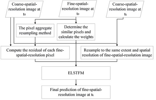
2.4. Implementation Process of ELSTFM

In practice, two coarse-spatial-resolution images obtained at the reference date (t0) and prediction date (tk) as well as one fine-spatial-resolution image acquired at t0 are necessary for fine-spatial-resolution image prediction. ELSTFM implementation mainly contains three steps: (1) the fine-spatial-resolution image at t0 is first resampled to the same spatial resolution of coarse-spatial-resolution image by utilizing the aggregate resampling approach, then the residuals of fine-spatial-resolution pixels can be computed based on Equations (10) and (11); (2) for a given fine-spatial-resolution pixel, the neighboring similar pixels and their corresponding weights are calculated, and the coarse-spatial-resolution images at t0 and tk are resampled to the same spatial resolution of the fine-spatial-resolution image; and (3) the ELSTFM is utilized to synthesize the final fine-spatial-resolution image at tk based on Equation (6). The flowchart of the ELSTFM is shown in Figure 1.

3. Experiments

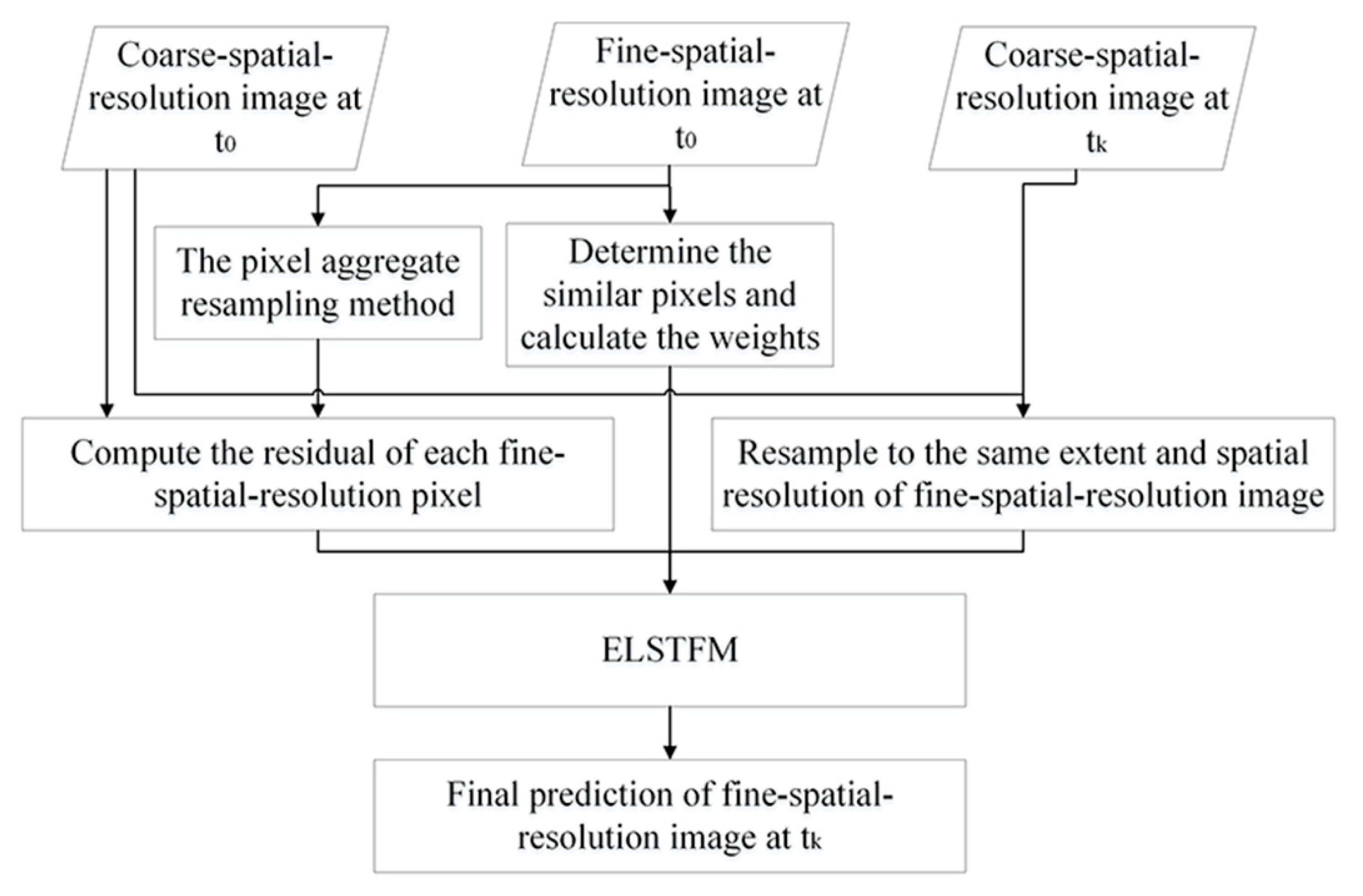
3.1. Experimental Data and Pre-Processing

To better compare with the existing fusion methods, similar to previous studies, two typical study sites of Landsat-7/ETM+ and 8-day composite 500-m resolution MODIS surface reflectance products (MOD09A1) data which have been used to validate STARFM, ESTARFM, and FSDAF algorithms [29,37] were selected. Landsat-7/ETM+ and MODIS sensors can acquire images of a roughly 185 km × 185 km area and 2330 km (cross track) × 10 km (along track at nadir) area, respectively. The 8-day composite MODIS data instead of daily MODIS data were used because of their relatively high data quality. These two kinds of data can be downloaded from the United States Geological Survey (USGS) EarthExplorer (http://glovis.usgs.gov/) and the National Aeronautics and Space Administration (NASA) (https://modis.gsfc.nasa.gov/), respectively.
The NIR–red–green as the RGB composite of Landsat-7/ETM+ images and their corresponding MODIS images of the first site with heterogeneous landscape is shown in Figure 2. We used two cloud-free Landsat-7/ETM+ images (Path/Row 93/84) acquired on 11 January (Figure 2a, used as input fine-spatial-resolution image) and 12 February 2002 (Figure 2b, used to validate the experimental accuracy) with six bands (the 1st–5th bands and the 7th band) covering an area of approximately 24 × 15 km2 (800 × 496 fine-spatial-resolution pixels) in southern New South Wales, Australia (145°E, 34°S). This heterogonous site can be deemed as a benchmark for comparing or testing spatio-temporal fusion methods and has been widely used in spatio-temporal fusion studies. The major land cover types in this area are irrigated rice cropland, dryland agriculture, and woodlands. Meanwhile, two MOD09A1 images acquired on 9 January (Figure 2c, used as the coarse-spatial-resolution image at the reference date) and 10 February 2002 (Figure 2d, used as the coarse-spatial-resolution image at the prediction date) with six bands (the 1st–4th bands and 6th and 7th bands) covering the same area (h29v12) were selected.
The second site was located in Canada (54°N, 104°W), covering an area of approximate 11.5 × 17.7 km2 (384 × 592 fine-spatial-resolution pixels), where the growing season is short and phenology changes are extreme [13]. The major land-cover in this region is forest, with subsidiary fen and patches of sparse vegetation (soil, rock, burn scars). This site has been used to validate the STARFM method and can be regarded as a homogenous area. The NIR–red–green as the RGB composite of the Landsat-7/ETM+ images and their corresponding MODIS images are shown in Figure 3. Two Landsat-7/ETM+ images (Path/Row 36/22) acquired on 17 May (Figure 3a, used as input fine-spatial-resolution image) and 2 June 2001 (Figure 3b, used to validate the experimental accuracy) with six bands (the 1st–5th bands and the 7th band) utilized. Additionally, the two input MOD09A1 images (h11v03) with six bands (the 1st–4th bands and the 6th and 7th bands) at the reference and prediction dates were acquired on 17 May (Figure 3c) and 2 June 2001 (Figure 3d), respectively.
All experimental fine- and coarse-spatial-resolution images were preprocessed before predicting the synthetic image. The Landsat ecosystem disturbance adaptive processing system (LEDAPS) was employed to atmospherically correct and calibrate the digital numbers from the Landsat level 1 product. The Landsat-7/ETM+ and MODIS surface reflectance data can be deemed as consistent and comparable because of the same atmospheric correction approach used for Landsat and MODIS data [13,29]. Additionally, the ISODATA method was used in this study to generate the classification maps of the two study sites to meet the requirements of the FSDAF algorithm.
By utilizing the MODIS reprojection tool (MRT), the MOD09A1 images were first reprojected to the universal transverse mercator (UTM) projection, then resampled to a 30 m spatial resolution based on the nearest neighbor method, and finally clipped to the same extent of the Landsat-7/ETM+ images for the two study sites. For convenience, to match 16 times the spatial resolution of the Landsat images, the MODIS at 500 m resolution were resampled into 480 m by using the nearest neighbor approach. The bandwidths of MODIS and Landsat-7/ETM+ data were similar even though the bandwidths of MODIS data were narrower than those of Landsat-7/ETM+ data (Table 1).

3.2. Quantitative Comparison

The performance of ELSTFM was quantitatively and visually compared with the Fit_FC algorithm [12], FSDAF algorithm [29], and STARFM algorithm [13]. These algorithms are based on either a linear model or the unmixing model and have been widely used. Five indices including the correlation coefficient (γ), root mean square error (RMSE), structural similarity index (SSIM), average absolute difference (AAD), and ERGAS were used to evaluate these four fusion methods. The higher ɤ indicates better linear correlativity between the predicted and actual data; SSIM can assess the similarity of the overall structure (the best value is 1); lower RMSE and AAD values represent better fusion performance of the corresponding method; and a lower ERGAS value means better image fusion quality. These metrics can be calculated as follows:
γ = a = 1 A ( k a k ¯ ) ( l a l ¯ ) a = 1 A ( k a k ¯ ) 2 a = 1 A ( l a l ¯ ) 2 S S I M = ( 2 k l ¯ + C 1 ) ( 2 σ k l + C 2 ) ( k ¯ 2 + l ¯ 2 + C 1 ) ( σ k + σ l + C 2 ) R M S E = a = 1 A ( k a l a ) 2 A A A D = 1 A a = 1 A | k a l a | E R G A S = 100 r h r l 1 n u m _ b a n d B = 1 n u m _ b a n d ( R M S E B 2 / l ¯ B 2 )
where A denotes the total pixels number of fine-spatial-resolution image; ka and la are the values of the ath synthetic and actual fine-spatial-resolution pixels;   k ¯ and l ¯ are the mean values of the synthetic and actual images; rh and rl represent the resolutions of high and low spatial resolution images (in this paper, the spatial resolutions of Landsat-7/ETM+ data and MODIS data are set to 30 m and 480 m); RMSEB is the RMSE value of the Bth band between the synthetic and actual images; l ¯ B is the average value of the Bth band of the actual image; σk and σl are variances of the synthetic and actual images; σkl denotes the covariance of the synthetic and actual images; C1, C2 are two small constants to avoid outliers, and in this study, they are both equal to 0.001.

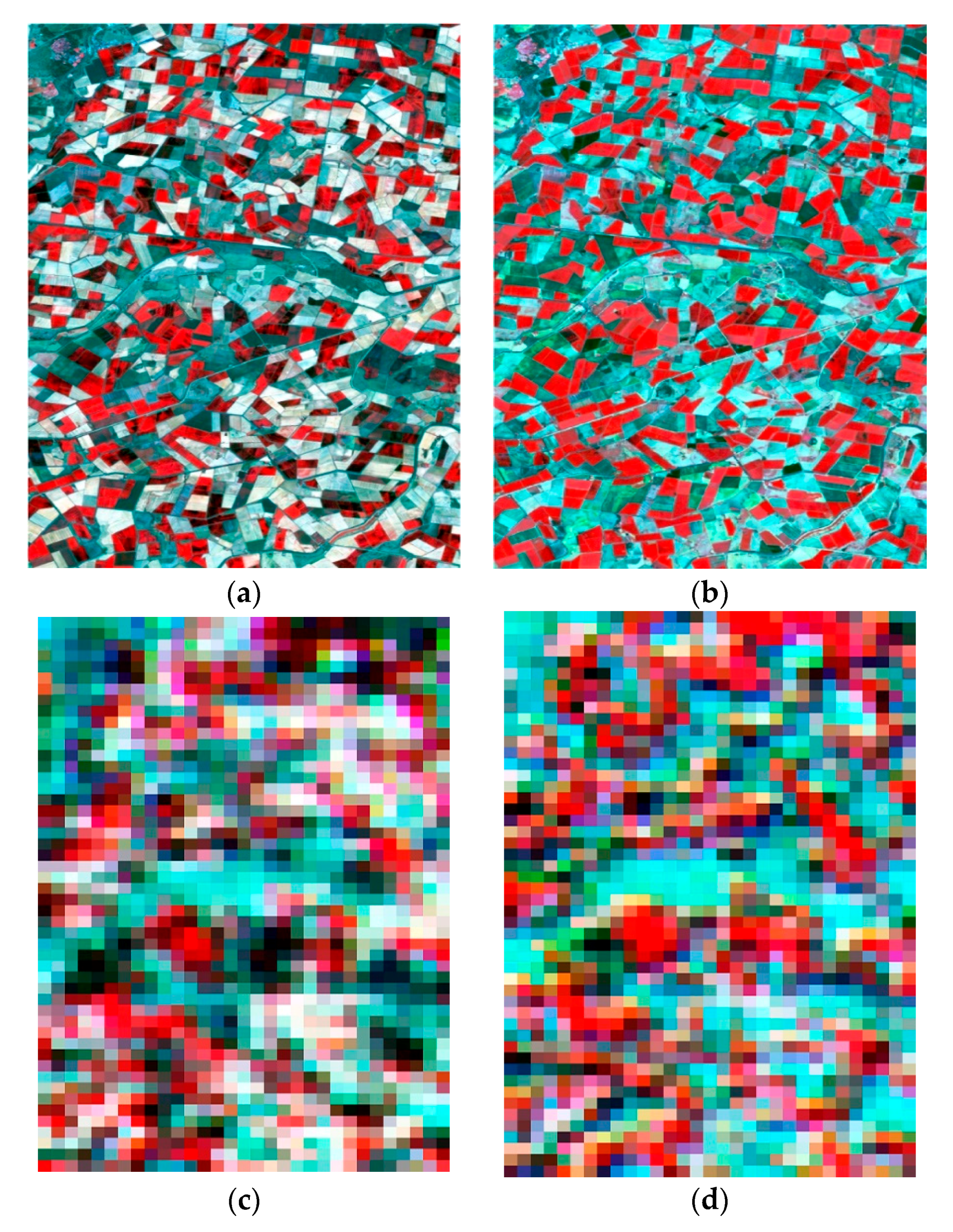
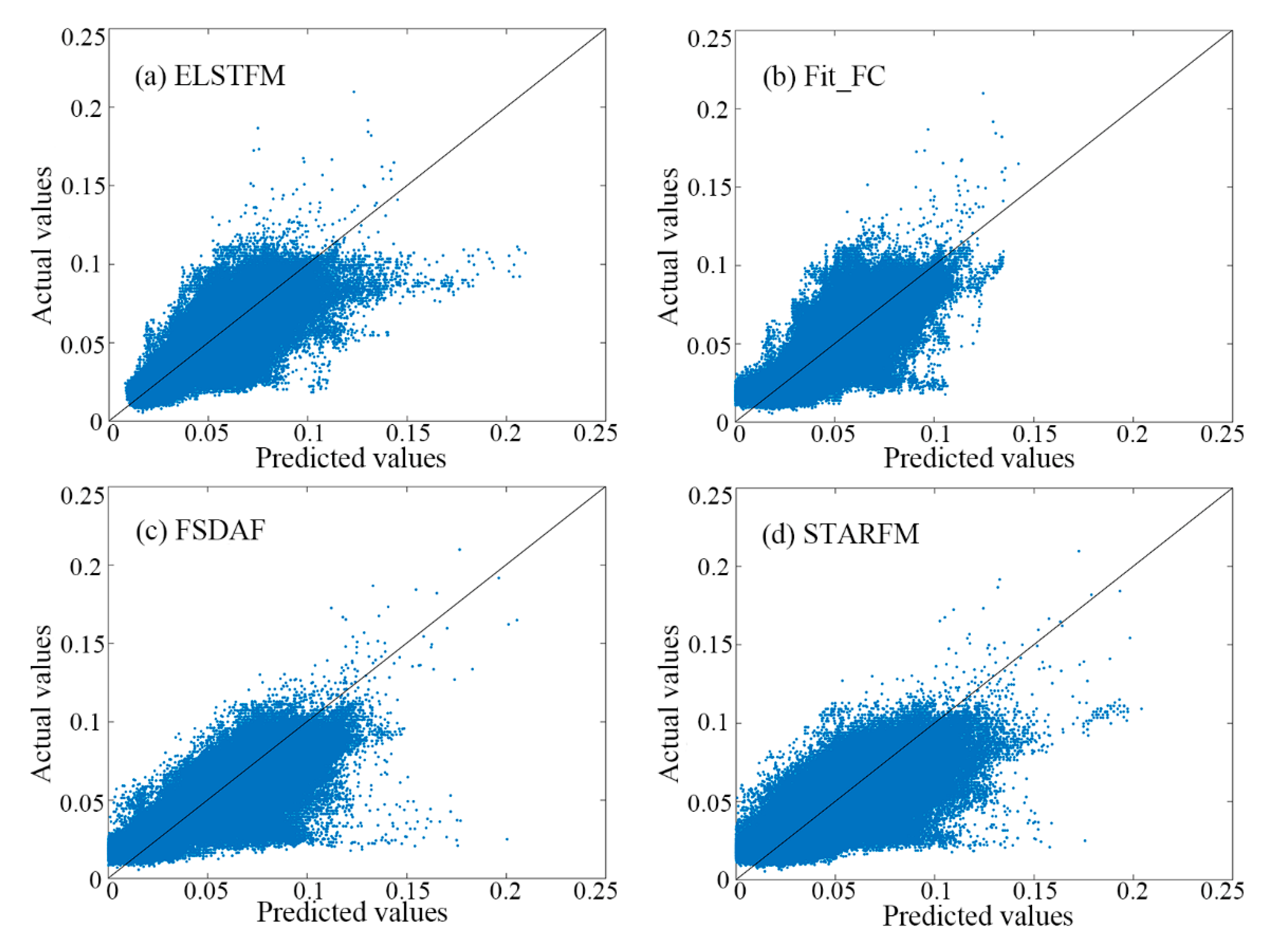
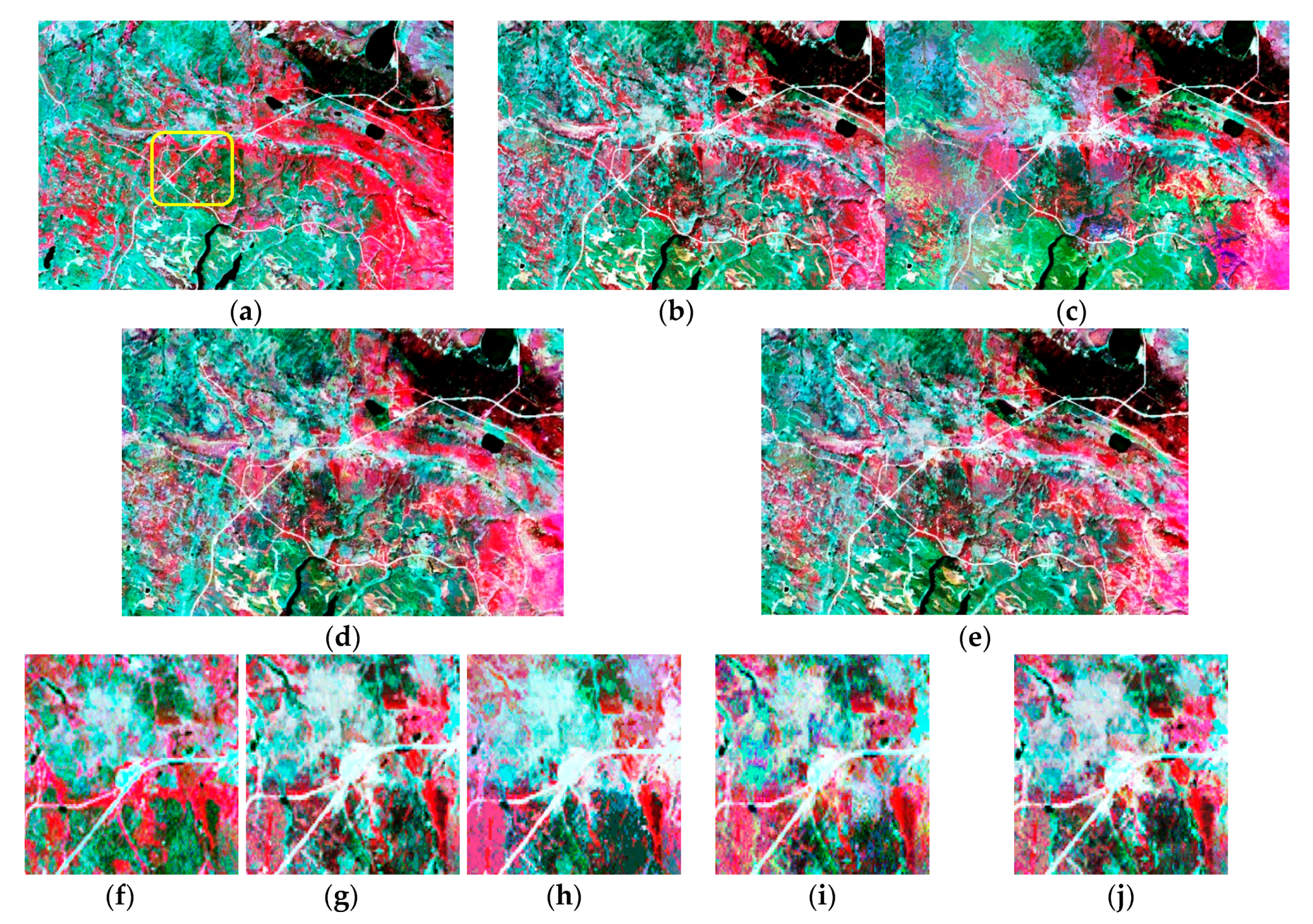
3.3. Results for Experimental Site 1

Figure 4b–e shows the predicted images on 12 February 2002 generated by the four data fusion methods and Figure 4a is the actual Landsat-7/ETM+ image acquired on 12 February 2002. A zoom-in area marked by the yellow square in Figure 4a was also used to highlight the difference between the predicted images and the actual image (Figure 4f–j). As a whole, from the visual comparison, the predicted images were all similar to the actual image in most regions. However, when compared with the other three methods, the predicted image obtained by ELSTFM was closer to the actual image with regard to the spatial details for some special regions such as the zoom-in images in Figure 4f–j. We can see that the images obtained by the FSDAF and STARFM methods could capture the main spatial details, however, some pixels were not appropriately predicted; the image obtained by the Fit_FC method seemed to be a little over-smooth such that some spatial details were missing, which may have resulted from the window size setting for coefficients fitting in Fit_FC.
We used the first band (blue band) of the Landsat-7/ETM+ data as an example to analyze the differences between the predicted values and actual values pixel-by-pixel. As shown in Figure 5, the scatter plots by the four methods confirmed that the values predicted by ELSTFM and Fit-FC seemed to be more accurate than the other two methods, which corresponded to the statistical results (Table 2) that ELSTFM and Fit-FC were the better fusion methods for the objective image. However, when compared with the other three methods, the ELSTFM could best predict the lower reflectance values, which can partly explain the best fusion accuracy obtained by ELSTFM method.
Table 2 shows the five quantitative indices calculated by comparing the predicted results based on the ELSTFM, Fit_FC, FSDAF, and STARFM methods with the actual Landsat-7/ETM+ image acquired on 12 February 2002. We can see that with the exception of band 2, the results of ELSTFM had the highest γ and smallest RMSE; for all six bands, the results of ELSTFM had the highest SSIM and smallest AAD; ERGASs obtained by ELSTFM, Fit_FC, FSDAF, and STARFM methods were 1.4943, 1.7561, 1.9920, and 1.9630, respectively. All statistical results suggested that ELSTFM could acquire the best fusion accuracy among these methods for site 1. Similar to previous studies [29], the NIR band had the largest difference in accuracy between the ELSTFM and the other three methods (γ 0.5786 vs. 0.3787, 0.4248 and 0.5262, SSIM 0.5931 vs. 0.4019, 0.4664, and 0.5598, RMSE 0.0655 vs. 0.0750, 0.0774, and 0.0719, AAD 0.0487 vs. 0.0569, 0.0591, and 0.0535). For all six bands, by using the ELSTFM method, the average enhancements of γ as well as SSIM were 0.0991, 0.0456, and 0.0462 as well as 0.0899, 0.0648, and 0.0496; and meanwhile, the mean decreases of RMSE as well as AAD were 0.0072, 0.0089, and 0.0077 as well as 0.0070, 0.0079, and 0.0063. Additionally, because actual MODIS data were utilized in this paper, the radiometric and geometric inconsistencies may lead to some differences between the results obtained in this study and a previous study which used simulated MODIS data [29].

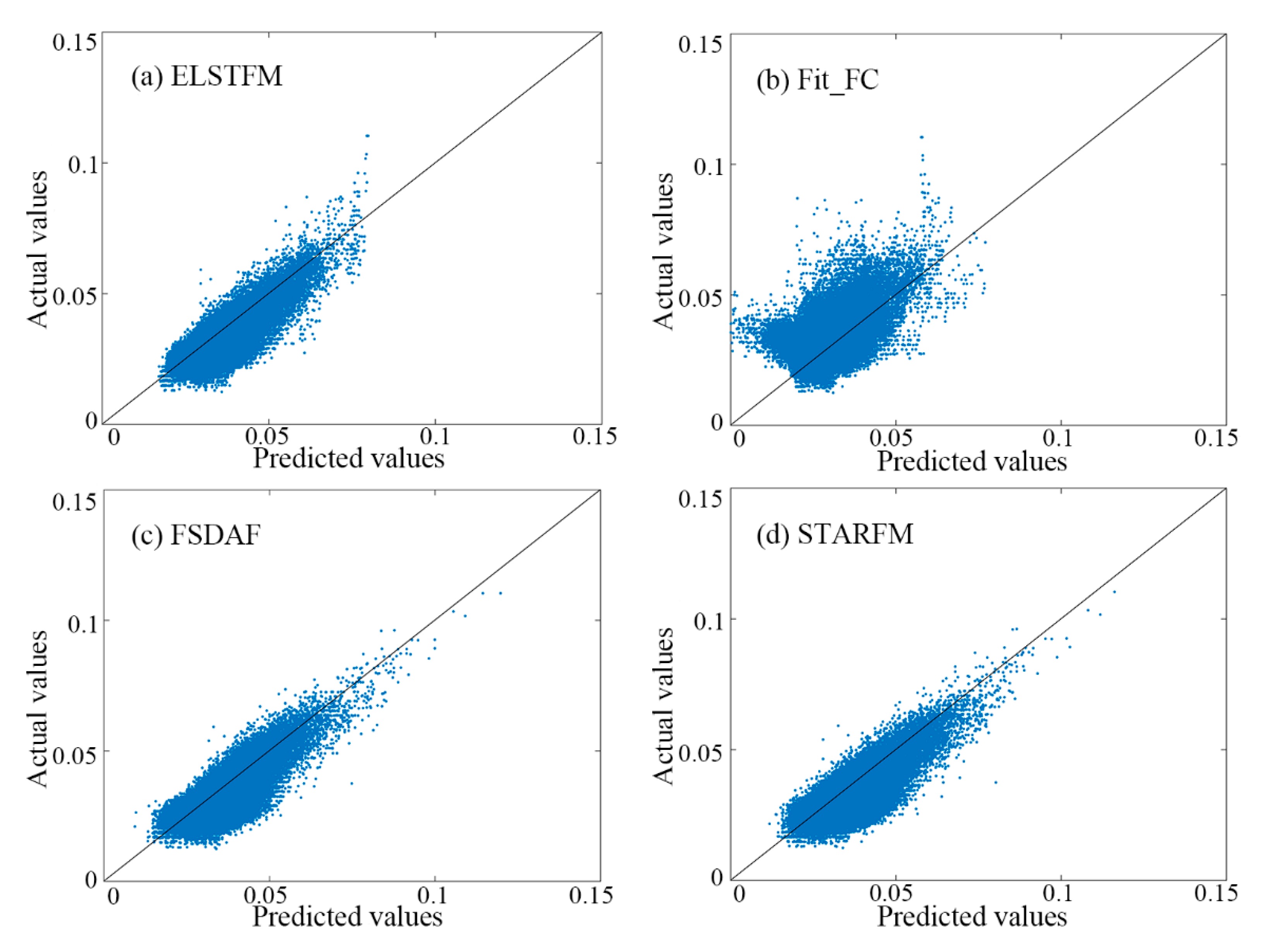
3.4. Results for Experimental Site 2

Figure 6b–e shows the predicted images for experimental site 2 on 2 June 2001 generated by the four data fusion methods and Figure 6a is the actual Landsat-7/ETM+ image acquired on 2 June 2001. A zoom-in area marked by the yellow square in Figure 6a was used to highlight the difference between the predicted images and the actual image (Figure 6f–j). Compared with site 1, site 2 seems to be more homogeneous. From the visual comparison, all these methods could acquire similar fusion results, but like the conclusions about site 1, the fused image obtained by the Fit_FC method seemed to be a little over-smooth and some details were missing; the differences between the results obtained by ELSTFM, FSDAF, and STARFM were not obvious (Figure 6f–j), suggesting that for the homogeneous region, all these methods could generate visually similar results.
Figure 7 shows the scatter plots of the actual vs. predicted blue band of the Landsat-7/ETM+ data by the four methods. As shown in Figure 7, the ELSTFM, FSDAF, and STARFM methods could obtain similar distributions, however, some predicted values from Fit_FC seemed to be a little lower than the actual values. Table 3 gives the accuracies obtained by the four fusion methods. For all six bands, the results of the ELSTFM had the highest ɤ and SSIM, suggesting that the ELSTFM method acquired the most accurate predicted images. Even though for bands 2, 3, and 7, the results of Fit_FC had the smallest RMSE and AAD, the differences between those values obtained by ELSTFM and Fit_FC were not obvious. Additionally, the ERGASs obtained by ELSTFM, Fit_FC, FSDAF, and STARFM were 0.9636, 1.0053, 1.0278, and 1.0638, respectively. In addition, by using the ELSTFM, the average enhancements of ɤ as well as SSIM were 0.0769, 0.0319, and 0.0222 as well as 0.0128, 0.0111, and 0.0092; the mean decreases of RMSE as well as AAD were 0.0002, 0.0007, and 0.0010 as well as 0.0005, 0.0010, and 0.0008.

4. Discussion

4.1. The Influences of the Resampling Algorithm

It is necessary to resample the original MODIS data to the same spatial resolution extent of the fine-spatial-resolution image in the ELSTFM method. Hence, the resampling method has a direct influence on the fusion accuracy of ELSTFM. In this part, we used the resampled 480 m spatial resolution MODIS images at the reference and prediction dates as the original input coarse-spatial-resolution images. Then, the thin plate spline (TPS) method, which has been used in a previous data fusion study [29], and the nearest neighbor interpolation (NNI) method were used to downscale the coarse-spatial-resolution images. Finally, the fusion accuracies based on different resampling methods were compared.
Table 4 gives the correlation coefficients between the resampled 30 m spatial resolution MODIS images obtained by the two resampling methods and the corresponding actual Landsat-7/ETM+ images for site 1 and site 2. We can see that for the two study sites, the correlation coefficients of all six bands obtained by the TPS method were all higher than those obtained by the NNI method. Additionally, the correlation coefficients of all six bands for site 2 were relatively higher than for site 1, suggesting that these two resampling methods could obtain better downscaled images for the homogeneous area.
Table 5 gives the accuracies of the ELSTFM applied to the resampled MODIS data obtained by the TPS and NNI methods for site 1 and site 2. The ERGASs using the TPS and NNI resampling methods were 1.5960 and 1.6132 for site 1, and 0.9883 and 0.9990 for site 2. We can see that for the two study sites, the results of all six bands based on the TPS resampling method were slightly better than the NNI method, suggesting that the resampling accuracy had positive effects on data fusion; on the other hand, the average differences between the results obtained by the two resampling methods were relatively small (γ: 0.0033 and 0.0032, SSIM: 0.0026 and 0.0015, RMSE: 0.0003 and 0.0002, AAD: 0.0002 and 0.0001), suggesting that the resampling method could slightly, but not significantly influence fusion accuracy.

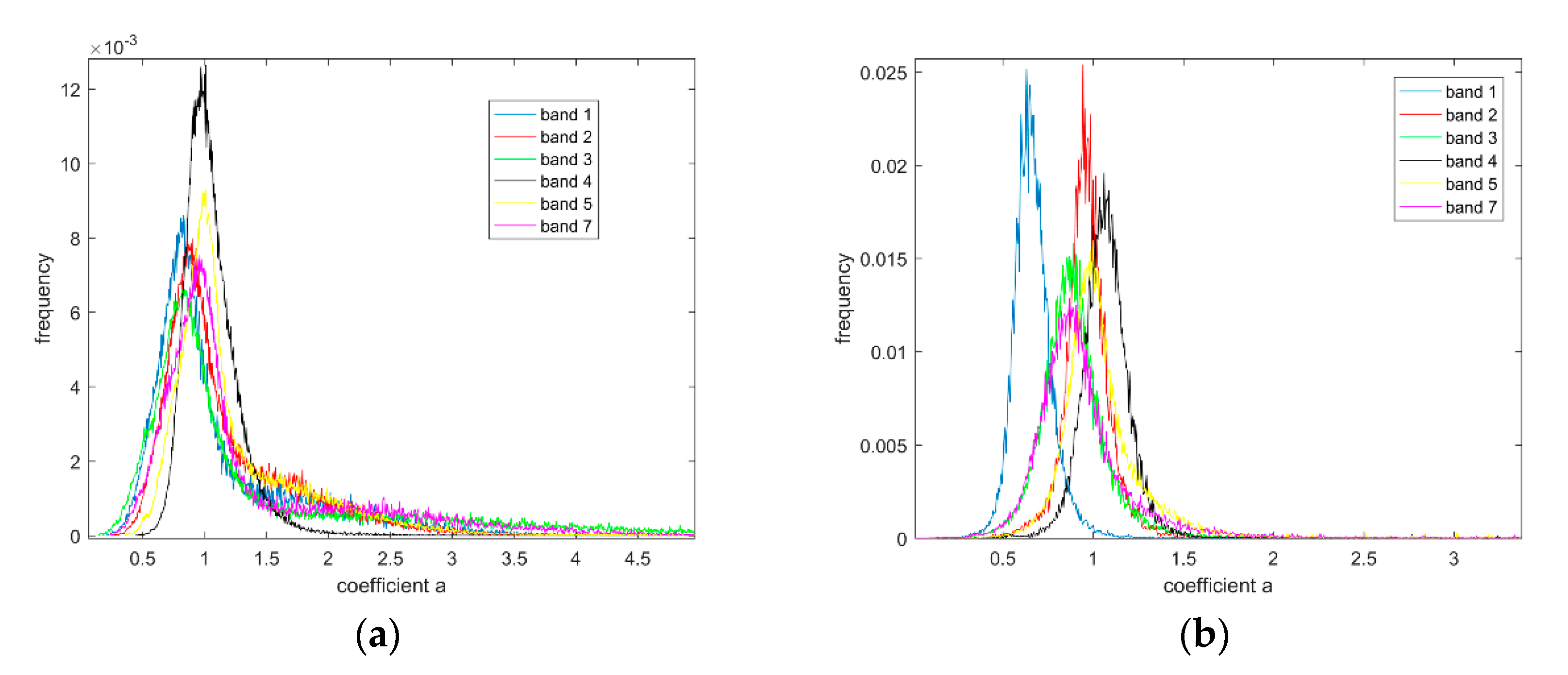
4.2. The Distributions of Slopes in ELSTFM

The slope of the linear model formed using Landsat and MODIS data should be close to 1 because these two datasets are consistent and comparable after the same atmospheric correction process [13,29]. Hence, in this part, we checked the distributions of the slopes of all six bands for two study sites to validate the ELSTFM indirectly. According to Equation (2), the slope of a pixel (m, n) can be calculated as:
a ( m , n , t 0 , B ) = M ( m , n , t 0 , B ) b ( m , n , t 0 , B ) L ( m , n , t 0 , B )
The mean values of the slopes of all six bands for site 1 were 1.1243, 1.1683, 1.4271, 1.0572, 1.2441, and 1.3384, respectively; and for site 2 were 0.6697, 0.9752, 0.9020, 1.1212, 1.1378, and 0.9735, respectively. The distributions of the slopes of all six bands for the two sites are shown in Figure 8. As shown in Figure 8a, all distributions of the slopes seemed to be normal distributions with the mean value of 1; similarly, for site 2, except for band 1, the distributions of the slopes of the other five bands were also normal distributions with a mean value close to 1. Both the mean values and the distributions of the slopes could confirm that the slope of line model was close to 1 because of the consistency between the Landsat and MODIS data; meanwhile, as the ELSTFM could get better fusion accuracies at different study sites, the changeable slope may enhance the fusion methods. Furthermore, we could see that the slopes of all six bands for the heterogeneous region (site 1) were higher than for the homogenous region, suggesting that the differences between Landsat-7/ETM+ and MODIS data may be relatively large in heterogeneous landscapes.

4.3. The Applicability of ELSTFM

Landsat-7/ETM+ data are seriously influenced by the scan line corrector problem after 2003 and currently, the eighth satellite in the series of Landsat satellite, Landsat-8, will continue and advance the collection of Landsat data. Hence, even though Landsat-7/ETM+ and MODIS data were used in this paper to validate the ELSTFM method, the ELSTFM can also be used for other satellite data such as Landsat-8/OLI and Sentinel series data. Additionally, because ELSTFM is a pixel-based method, even though the reflectance data were used to validate the proposed method, we believe it can also accurately predict any products derived from reflectance data, such as the leaf area index (LAI), normalized difference vegetation index (NDVI), and the normalized difference water index (NDWI).
The ELSTFM is based on a linear model, yet, different from the STARFM and ESTARFM, which deem the slope as either 1 or a constant, the slope of the linear model in the ELSTFM is changeable. However, if we assume the slope is equal to 1 and invariable, by subtraction of Equations (2) and (3), the intercept of the linear model can be eliminated, hence the proposed method can be transformed to the STARFM method. Through the experiments in the two study sites, the ELSTFM method could acquire better fusion results than the STARFM method. Hence, the ELSTFM can be deemed as an enhanced version of STARFM.

5. Conclusions

An enhanced linear spatio-temporal fusion model (ELSTFM) was proposed in this paper to generate data with both high spatial resolution and temporal frequency. The residuals of the fine-spatial-resolution pixels were first calculated based on spectral unmixing theory; the similar pixels and their corresponding weights were then computed; after that, the coarse-spatial-resolution images at the reference and prediction dates were resampled to the same spatial resolution and extent of the fine-spatial-resolution images; finally, the ELSTFM was employed to synthesize the fine-spatial-resolution image at the prediction date. Through the comparisons between ELSTFM and three other typical spatio-temporal fusion methods (Fit_FC, FSDAF, and STARFM), for the two study sites, the ELSTFM could acquire better fusion accuracies.
Additionally, the performances of the ELSTFM based on different resampling methods for the two study sites were examined. The resampling methods can slightly, but not significantly influence the ELSTFM method. Moreover, for most bands, the distributions of the slopes of the linear model for the two study sites were normal distributions with a mean value of 1. In addition, the ELSTFM was designed to synthesize not only the reflectance data, but also the satellite products derived from the reflectance data.
Some factors that can limit the performance of ELSTFM still exist and need to be overcome. The fine-spatial-resolution pixels are predicted pixel-by-pixel in the ELSTFM, and even though the neighboring similar pixels are used to decrease the influences of heterogeneity, the radiometric and atmospheric errors can seriously affect fusion accuracy. In addition, the residuals of the fine-spatial-resolution pixels are calculated by using the spectral unmixing theory in the ELSTFM, yet some errors still exist. Some other methods that can enhance the accuracies of the residuals can definitely improve the performance of the ELSTFM method.
Additionally, this research aimed to enhance the spatio-temporal fusion based on the linear model and the coefficients a and b were determined locally in this paper, which means they were regarded as temporally invariable in a short period. However, when the temporal gap between the acquisitions of input images is relatively large, which may result in large landscapes changes, these two coefficients should be determined locally and temporally.

Author Contributions

P.B. was responsible for designing the study, processing datasets, building the model and writing the original paper; M.Y. and S.F. were responsible for the supervision, writing-review and editing.

Funding

This research received no external funding.

Conflicts of Interest

The authors declare no conflict of interest.

References

  1. Du, P.J.; Liu, S.C.; Xia, J.S.; Zhao, Y.D. Information fusion techniques for change detection from multi-temporal remote sensing images. Inf. Fusion 2013, 14, 19–27. [Google Scholar] [CrossRef]
  2. Fu, D.J.; Chen, B.Z.; Zhang, H.F.; Wang, J.; Black, T.A.; Amiro, B.D.; Bohrer, G.; Bolstad, P.; Coulter, R.; Rahman, A.F.; et al. Estimating landscape net ecosystem exchange at high spatial-temporal resolution based on Landsat data, an improved upscaling model framework, and eddy covariance flux measurements. Remote Sens. Environ. 2014, 141, 90–104. [Google Scholar] [CrossRef]
  3. Gong, P.; Wang, J.; Yu, L.; Zhao, Y.C.; Zhao, Y.Y.; Liang, L.; Niu, Z.G.; Huang, X.M.; Fu, H.H.; Liu, S.; et al. Fine resolution observation and monitoring of global land cover: First mapping results with Landsat TM and ETM+ data. Int. J. Remote Sens. 2013, 34, 2607–2654. [Google Scholar] [CrossRef]
  4. Jia, K.; Liang, S.L.; Zhang, N.; Wei, X.Q.; Gu, X.F.; Zhao, X.; Yao, Y.J.; Xie, X.H. Land cover classification of finer resolution remote sensing data integrating temporal features from time series coarser resolution data. ISPRS J. Photogramm. Remote Sens. 2014, 93, 49–55. [Google Scholar] [CrossRef]
  5. Leckie, D.G. Advances in remote-sensing technologies for forest surveys and management. Can. J. For. Res. 1990, 20, 464–483. [Google Scholar] [CrossRef]
  6. Asner, G.P. Cloud cover in Landsat observations of the Brazilian Amazon. Int. J. Remote Sens. 2001, 22, 3855–3862. [Google Scholar] [CrossRef]
  7. Carrao, H.; Goncalves, P.; Caetano, M. Contribution of multispectral and multiternporal information from MODIS images to land cover classification. Remote Sens. Environ. 2008, 112, 986–997. [Google Scholar] [CrossRef]
  8. Kim, Y.; Kimball, J.S.; Didan, K.; Henebry, G.M. Response of vegetation growth and productivity to spring climate indicators in the conterminous United States derived from satellite remote sensing data fusion. Agric. For. Meteorol. 2014, 194, 132–143. [Google Scholar] [CrossRef]
  9. Thenkabail, P.S.; Schull, M.; Turral, H. Ganges and Indus river basin land use/land cover (LULC) and irrigated area mapping using continuous streams of MODIS data. Remote Sens. Environ. 2005, 95, 317–341. [Google Scholar] [CrossRef]
  10. Zhang, X.; Sun, R.; Zhang, B.; Tong, Q.X. Land cover classification of the North China Plain using MODIS_EVI time series. ISPRS J. Photogramm. Remote Sens. 2008, 63, 476–484. [Google Scholar] [CrossRef]
  11. Zhu, X.L.; Chen, J.; Gao, F.; Chen, X.H.; Masek, J.G. An enhanced spatial and temporal adaptive reflectance fusion model for complex heterogeneous regions. Remote Sens. Environ. 2010, 114, 2610–2623. [Google Scholar] [CrossRef]
  12. Wang, Q.M.; Atkinson, P.M. Spatio-temporal fusion for daily Sentinel-2 images. Remote Sens. Environ. 2018, 204, 31–42. [Google Scholar] [CrossRef]
  13. Gao, F.; Masek, J.; Schwaller, M.; Hall, F. On the blending of the Landsat and MODIS surface reflectance: Predicting daily Landsat surface reflectance. IEEE Trans. Geosci. Remote Sens. 2006, 44, 2207–2218. [Google Scholar]
  14. Hilker, T.; Wulder, M.A.; Coops, N.C.; Linke, J.; McDermid, G.; Masek, J.G.; Gao, F.; White, J.C. A new data fusion model for high spatial- and temporal-resolution mapping of forest disturbance based on Landsat and MODIS. Remote Sens. Environ. 2009, 113, 1613–1627. [Google Scholar] [CrossRef]
  15. Dong, T.F.; Liu, J.G.; Qian, B.D.; Zhao, T.; Jing, Q.; Geng, X.Y.; Wang, J.F.; Huffman, T.; Shang, J.L. Estimating winter wheat biomass by assimilating leaf area index derived from fusion of Landsat-8 and MODIS data. Int. J. Appl. Earth Obs. Geoinf. 2016, 49, 63–74. [Google Scholar] [CrossRef]
  16. Shen, H.F.; Huang, L.W.; Zhang, L.P.; Wu, P.H.; Zeng, C. Long-term and fine-scale satellite monitoring of the urban heat island effect by the fusion of multi-temporal and multi-sensor remote sensed data: A 26-year case study of the city of Wuhan in China. Remote Sens. Environ. 2016, 172, 109–125. [Google Scholar] [CrossRef]
  17. Weng, Q.H.; Fu, P.; Gao, F. Generating daily land surface temperature at Landsat resolution by fusing Landsat and MODIS data. Remote Sens. Environ. 2014, 145, 55–67. [Google Scholar] [CrossRef]
  18. Zhu, L.K.; Radeloff, V.C.; Ives, A.R. Improving the mapping of crop types in the Midwestern U.S. by fusing Landsat and MODIS satellite data. Int. J. Appl. Earth Obs. Geoinf. 2017, 58, 1–11. [Google Scholar] [CrossRef]
  19. Gao, F.; Hilker, T.; Zhu, X.; Anderson, M.; Masek, J.G.; Wang, P.; Yang, Y. Fusing Landsat and MODIS data for vegetation monitoring. IEEE Geosci. Remote Sens. Mag. 2015, 3, 47–60. [Google Scholar] [CrossRef]
  20. Gao, F.; Anderson, M.C.; Zhang, X.Y.; Yang, Z.W.; Alfieri, J.G.; Kustas, W.P.; Mueller, R.; Johnson, D.M.; Prueger, J.H. Toward mapping crop progress at field scales through fusion of Landsat and MODIS imagery. Remote Sens. Environ. 2017, 188, 9–25. [Google Scholar] [CrossRef]
  21. Kong, F.J.; Li, X.B.; Wang, H.; Xie, D.F.; Li, X.; Bai, Y.X. Land Cover Classification Based on Fused Data from GF-1 and MODIS NDVI Time Series. Remote Sens. 2016, 8, 741. [Google Scholar] [CrossRef]
  22. Huang, C.; Chen, Y.; Zhang, S.Q.; Li, L.Y.; Shi, K.F.; Liu, R. Surface water mapping from Suomi NPP-VIIRS imagery at 30 m resolution via blending with Landsat data. Remote Sens. 2016, 8, 631. [Google Scholar] [CrossRef]
  23. Cheng, Q.; Liu, H.Q.; Shen, H.F.; Wu, P.H.; Zhang, L.P. A spatial and temporal nonlocal filter-based data fusion method. IEEE Trans. Geosci. Remote Sens. 2017, 55, 4476–4488. [Google Scholar] [CrossRef]
  24. Zurita-Milla, R.; Kaiser, G.; Clevers, J.G.P.W.; Schneider, W.; Schaepman, M.E. Downscaling time series of MERIS full resolution data to monitor vegetation seasonal dynamics. Remote Sens. Environ. 2009, 113, 1874–1885. [Google Scholar] [CrossRef]
  25. Gevaert, C.M.; Garcia-Haro, F.J. A comparison of STARFM and an unmixing-based algorithm for Landsat and MODIS data fusion. Remote Sens. Environ. 2015, 156, 34–44. [Google Scholar] [CrossRef]
  26. Xie, D.F.; Zhang, J.S.; Zhu, X.F.; Pan, Y.Z.; Liu, H.L.; Yuan, Z.M.Q.; Yun, Y. An Improved STARFM with help of an unmixing-based method to generate high spatial and temporal resolution remote sensing data in complex heterogeneous regions. Sensors 2016, 16, 207. [Google Scholar] [CrossRef] [PubMed]
  27. Wu, M.Q.; Niu, Z.; Wang, C.Y.; Wu, C.Y.; Wang, L. Use of MODIS and Landsat time series data to generate high-resolution temporal synthetic Landsat data using a spatial and temporal reflectance fusion model. J. Appl. Remote Sens. 2012, 6. [Google Scholar] [CrossRef]
  28. Wu, M.Q.; Wu, C.Y.; Huang, W.J.; Niu, Z.; Wang, C.Y.; Li, W.; Hao, P.Y. An improved high spatial and temporal data fusion approach for combining Landsat and MODIS data to generate daily synthetic Landsat imagery. Inf. Fusion 2016, 31, 14–25. [Google Scholar] [CrossRef]
  29. Zhu, X.L.; Helmer, E.H.; Gao, F.; Liu, D.S.; Chen, J.; Lefsky, M.A. A flexible spatiotemporal method for fusing satellite images with different resolutions. Remote Sens. Environ. 2016, 172, 165–177. [Google Scholar] [CrossRef]
  30. Rao, Y.H.; Zhu, X.L.; Chen, J.; Wang, J.M. An Improved Method for Producing High Spatial-Resolution NDVI Time Series Datasets with Multi-Temporal MODIS NDVI Data and Landsat TM/ETM plus Images. Remote Sens. 2015, 7, 7865–7891. [Google Scholar] [CrossRef]
  31. Wu, M.Q.; Huang, W.J.; Niu, Z.; Wang, C.Y.; Li, W.; Yu, B. Validation of synthetic daily Landsat NDVI time series data generated by the improved spatial and temporal data fusion approach. Inf. Fusion 2018, 40, 34–44. [Google Scholar] [CrossRef]
  32. Amorós-López, J.; Gómez-Chova, L.; Alonso, L.; Guanter, L.; Zurita-Milla, R.; Moreno, J.; Camps-Valls, G. Multitemporal fusion of Landsat/TM and ENVISAT/MERIS for crop monitoring. Int. J. Appl. Earth Obs. Geoinf. 2013, 23, 132–141. [Google Scholar] [CrossRef]
  33. Huang, B.; Song, H. Spatiotemporal reflectance fusion via sparse representation. IEEE Trans. Geosci. Remote Sens. 2012, 50, 3707–3716. [Google Scholar] [CrossRef]
  34. Song, H.; Huang, B. Spatiotemporal satellite image fusion through one-pair image learning. IEEE Trans. Geosci. Remote Sens. 2013, 51, 1883–1896. [Google Scholar] [CrossRef]
  35. Liu, X.; Deng, C.; Wang, S.; Huang, G.; Zhao, B.; Lauren, P. Fast and accurate spatiotemporal fusion based upon extreme learning machine. IEEE Geosci. Remote Sens. Lett. 2016, 13, 2039–2043. [Google Scholar] [CrossRef]
  36. Das, M.; Ghosh, S.K. Deep-STEP: A deep learning approach for spatiotemporal prediction of remote sensing data. IEEE Geosci. Remote Sens. Lett. 2016, 13, 1984–1988. [Google Scholar] [CrossRef]
  37. Emelyanova, I.V.; McVicar, T.R.; Van Niel, T.G.; Li, L.T.; van Dijk, A.I.J.M. Assessing the accuracy of blending Landsat-MODIS surface reflectances in two landscapes with contrasting spatial and temporal dynamics: A framework for algorithm selection. Remote Sens. Environ. 2013, 133, 193–209. [Google Scholar] [CrossRef]
Figure 1. Flowchart of the enhanced linear spatio-temporal fusion method (ELSTFM) algorithm.
Remotesensing 10 00881 g001
Figure 2. Test data of site 1: Landsat-7/ETM+ images (800 × 496 pixels) acquired on (a) 11 January 2002 and (b) 12 February 2002 as well as 8-day composite MODIS images resampled to 480 m resolution (50 × 31 pixels) acquired on (c) 9 January 2002, and (d) 10 February 2002. All images used NIR–red–green as RGB and identical linear stretches.
Remotesensing 10 00881 g002
Figure 3. Test data of site 2: Landsat-7/ETM+ images (384 × 592 pixels) acquired on (a) 17 May 2001 and (b) 2 June 2001 as well as 8-day composite MODIS images resampled to 480 m resolution (24 × 37 pixels) acquired on (c) 17 May 2001, and (d) 2 June 2001. All images used NIR–red–green as RGB and identical linear stretches.
Remotesensing 10 00881 g003
Figure 4. Results obtained from the (b) ELSTFM algorithm; (c) Fit_FC algorithm; (d) FSDAF algorithm; and (e) STARFM algorithm for site 1 (NIR, red, green bands as RGB) on 12 February 2002. (a,f) are the actual Landsat-7/ETM+ image and the subarea marked in yellow in (a) on 12 February 2002. (gj) are the corresponding results on 12 February 2002 for the subarea marked in yellow in (a).
Remotesensing 10 00881 g004
Figure 5. Scatter plots of actual and predicted values obtained by using (a) ELSTFM; (b) Fit_FC; (c) FSDAF; and (d) STARFM for the blue band of Figure 4a, and the line is the 1:1 line.
Remotesensing 10 00881 g005
Figure 6. Results obtained from the (b) ELSTFM algorithm, (c) Fit_FC algorithm, (d) FSDAF algorithm, and (e) STARFM algorithm for site 2 (NIR, red, green bands as RGB) on 2 June 2001. (a,f) are the actual Landsat-7/ETM+ image and the subarea marked in yellow on 2 June 2001. (gj) are the corresponding results on 2 June 2001 for the subarea marked in yellow in (a).
Remotesensing 10 00881 g006
Figure 7. Scatter plots of actual and predicted values obtained by using (a) ELSTFM; (b) Fit_FC; (c) FSDAF; and (d) STARFM for the blue band of Figure 6a, and the line is the 1:1 line.
Remotesensing 10 00881 g007
Figure 8. The distributions of the slopes of all six bands for site 1 (a) and site 2 (b).
Remotesensing 10 00881 g008
Table 1. Landsat-7/ETM+ and MODIS bandwidths.
Landsat-7/ETM+ BandLandsat-7/ETM+ Bandwidth (nm)MODIS BandMODIS Bandwidth (nm)
1450–5203459–479
2530–6104545–565
3630–6901620–670
4780–9002841–876
51550–175061628–1652
72090–235072105–2155
Table 2. The fusion accuracies obtained from four data fusion methods for study site 1 (Figure 4). The units are reflectance.
Band 1Band 2Band 3Band 4Band 5Band 7
ɤELSTFM0.87690.83310.87210.57860.89830.8971
Fit_FC0.85690.78700.84560.37870.80650.6867
FSDAF0.87400.83500.86230.42480.85600.8303
STARFM0.84320.77890.81500.52620.85520.8602
SSIMELSTFM0.93700.88680.89100.59310.90500.9043
Fit_FC0.93000.86830.87320.40190.80570.6983
FSDAF0.91850.83010.81310.46640.86110.8390
STARFM0.90550.82250.80060.55980.86100.8700
RMSEELSTFM0.01130.01830.02570.06550.03790.0357
Fit_FC0.01170.01820.02600.07500.04990.0568
FSDAF0.01360.02540.04050.07740.04790.0433
STARFM0.01470.02480.03990.07190.04780.0417
AADELSTFM0.00780.01260.01760.04870.02610.0244
Fit_FC0.00870.01350.01930.05690.03710.0437
FSDAF0.00980.01870.03020.05910.03430.0327
STARFM0.01050.01780.02880.05350.03410.0303
Table 3. The fusion accuracies obtained from four data fusion methods for study site 2 (Figure 6). The units are reflectance.
Band 1Band 2Band 3Band 4Band 5Band 7
γELSTFM0.74660.86890.79920.81920.90960.8417
Fit_FC0.47640.81560.73160.79300.89830.8085
FSDAF0.70260.83680.75370.80950.89010.8012
STARFM0.70340.85330.76920.81810.89980.8081
SSIMELSTFM0.97860.98250.95250.85390.92630.8970
Fit_FC0.96000.97930.94420.82790.92080.8817
FSDAF0.97540.98000.94330.83670.91560.8730
STARFM0.97420.98090.94160.85180.91830.8689
RMSEELSTFM0.00560.00530.00880.02410.02060.0185
Fit_FC0.00710.00520.00840.02500.02070.0177
FSDAF0.00590.00530.00950.02440.02140.0204
STARFM0.00600.00530.00990.02410.02180.0219
AADELSTFM0.00430.00400.00630.01700.01430.0130
Fit_FC0.00550.00380.00590.01830.01530.0128
FSDAF0.00450.00410.00700.01790.01630.0148
STARFM0.00450.00400.00710.01730.01560.0152
Table 4. The correlation coefficients between the resampled 30 m spatial resolution MODIS images obtained by two resampling methods and the corresponding actual Landsat-7/ETM+ images for site 1 and site 2. The units are reflectance. ref and pre represent the Landsat-7/ETM+ images at the reference and prediction dates.
Band 1Band 2Band 3Band 4Band 5Band 7
Site1TPSref0.38720.22380.25800.36670.33360.4027
pre0.40680.39100.28990.44220.32520.1883
NNIref0.34880.19880.23210.34030.30160.3769
pre0.36240.34710.25940.40310.28880.1726
Site2TPSref0.51510.49360.50800.49180.63150.5991
pre0.53220.45530.55220.63850.65270.6410
NNIref0.47760.45370.46980.44090.60210.5714
pre0.49310.41880.51630.59620.62330.6147
Table 5. Accuracy assessment of ELSTFM applied to the resampled MODIS data obtained by thin plate spline (TPS) and nearest neighbor interpolation (NNI) methods for site 1 and site 2. The units are reflectance.
Band 1Band 2Band 3Band 4Band 5Band 7
Site1TPSγ0.87800.84310.86940.46920.87830.8538
SSIM0.93870.88450.88620.50380.88610.8631
RMSE0.01110.01900.02650.07380.04170.0406
AAD0.00770.01310.01790.05560.02860.0289
NNIγ0.87490.83840.86540.46350.87580.8539
SSIM0.93710.88100.88250.49920.88370.8634
RMSE0.01120.01930.02710.07430.04220.0406
AAD0.00780.01320.01810.05590.02890.0288
Site2TPSγ0.72800.86650.78360.80520.90600.8295
SSIM0.97740.98220.94920.84410.92300.8887
RMSE0.00570.00540.00900.02500.02090.0192
AAD0.00430.00410.00650.01760.01460.0135
NNIγ0.72400.86540.78070.79850.90450.8267
SSIM0.97690.98200.94840.83980.92170.8866
RMSE0.00570.00540.00910.02530.02120.0194
AAD0.00440.00410.00650.01770.01480.0136

