Article

Mapping Urban Land Cover of a Large Area Using Multiple Sensors Multiple Features

1
Key Laboratory for Satellite Mapping Technology and Applications of State Administration of Surveying, Mapping and Geoinformation of China, Nanjing University, Nanjing 210093, China
2
Department of Geography, University of Wisconsin-Milwaukee, Milwaukee, WI 53211, USA
3
RIKEN Center for Advanced Intelligence Project, RIKEN, Tokyo 103-0027, Japan
4
Grenoble-Image-Speech-Signal-Automatics Laboratory (GIPSA)-Lab., Grenoble Institute of Technology, University Grenoble Alpes, 38400 Grenoble, France
*
Author to whom correspondence should be addressed.
Remote Sens. 2018, 10(6), 872; https://doi.org/10.3390/rs10060872
Submission received: 9 May 2018 / Revised: 29 May 2018 / Accepted: 30 May 2018 / Published: 5 June 2018

Abstract

:
Concerning the strengths and limitations of multispectral and airborne LiDAR data, the fusion of such datasets can compensate for the weakness of each other. This work have investigated the integration of multispectral and airborne LiDAR data for the land cover mapping of large urban area. Different LiDAR-derived features are involoved, including height, intensity, and multiple-return features. However, there is limited knowledge relating to the integration of multispectral and LiDAR data including three feature types for the classification task. Furthermore, a little contribution has been devoted to the relative importance of input features and the impact on the classification uncertainty by using multispectral and LiDAR. The key goal of this study is to explore the potenial improvement by using both multispectral and LiDAR data and to evaluate the importance and uncertainty of input features. Experimental results revealed that using the LiDAR-derived height features produced the lowest classification accuracy (83.17%). The addition of intensity information increased the map accuracy by 3.92 percentage points. The accuracy was further improved to 87.69% with the addition multiple-return features. A SPOT-5 image produced an overall classification accuracy of 86.51%. Combining spectral and spatial features increased the map accuracy by 6.03 percentage points. The best result (94.59%) was obtained by the combination of SPOT-5 and LiDAR data using all available input variables. Analysis of feature relevance demonstrated that the normalized digital surface model (nDSM) was the most beneficial feature in the classification of land cover. LiDAR-derived height features were more conducive to the classification of urban area as compared to LiDAR-derived intensity and multiple-return features. Selecting only 10 most important features can result in higher overall classification accuracy than all scenarios of input variables except the feature of entry scenario using all available input features. The variable importance varied a very large extent in the light of feature importance per land cover class. Results of classification uncertainty suggested that feature combination can tend to decrease classification uncertainty for different land cover classes, but there is no “one-feature-combination-fits-all” solution. The values of classification uncertainty exhibited significant differences between the land cover classes, and extremely low uncertainties were revealed for the water class. However, it should be noted that using all input variables resulted in relatively lower classification uncertainty values for most of the classes when compared to other input features scenarios.

Graphical Abstract

1. Introduction

Detailed knowledge of the land cover types and their aerial distribution are essential components for the management and conservation of the land resource and are of critical importance to a series of studies such as climate change assessment and policy purpose [1,2,3].
In recent decades, satellite remote sensing has exhibited its ability to achieve the land cover information with different temporal and spatial scales in the urban area. A multispectral satellite image can collect spectral information of land surfaces, and supply extra advantages to discriminate differences between urban land cover classes [4,5,6,7]. Even though many studies have successfully employed multispectral data for the classification of urban land cover, classification accuracy is more likely to be lower using spectral signature alone in the urban environment as compared to other environments such as forest environment. This is due to the fact that the urban environment possesses larger spectral and spatial heterogeneity of surface materials and the more complex pattern of land use [8]. In addition to devoting attention to the improving classification techniques, the development of input variables can be treated as an alternative way to improve the classification accuracy of a land cover map [7,9,10].
Aside from the spectral information, spatial features concerning geometric and textural, etc., have been incorporated into the classification of land cover. Many previous studies showed that the addition of spatial features had been found to be valuable for improving the performance [10,11,12,13]. In particular, spatial features derived from Attribute Profiles (APs) have attracted more attention in the classification due to the capabilities for providing the complementary information of spectral features [14,15]. APs is an extension of Morphological Profiles (MPs), aiming to overcome the limitation of MPs that is fit for providing multilevel variability of structures in an image. Recent studies performed the fusion of spectral and spatial features with extended APs, and pointed out its effectiveness [15,16]. While the classification result using the union of spectral and spatial features can present a good representation of urban land cover, some urban land cover types with similar materials prove difficult to be identified by using multispectral image alone. One solution could be to include an additional third dimension into the classification [9].
The availability of the Light Detection and Ranging (LiDAR) system succeeds to map vertical structure of surface objects. The LiDAR systems emit laser pulses using the wavelength in near infrared and record the returned laser pulse signals after backscattered from the targets [17,18,19]. The LiDAR system plays an increasingly vital role in the urban land cover mapping due to its power to acquire the vertical structure of surface objects with high positional accuracy. Different LiDAR-derived features can be extracted from LiDAR data, including LiDAR-derived height, intensity and multiple-return features [18,20,21]. LiDAR-derived features can describe the 3D topographic features of the earth surface, and a range of LiDAR-derived height features such as normalized DSM (nDSM) and height variation, has proved its help in improving map accuracy [18,20,22,23]. Intensity data as the radiometric component of LiDAR data, which is the peak backscattered laser energy from the illuminated object, can provide additional information for the land cover classification [24,25]. Song et al. [26] initially investigated the possibility of intensity data as the input features for the urban land cover mapping, and concluded that intensity data could be conducive to the land cover classification. In addition, a small number of researchers investigated the contribution of multiple-return features to the land cover classification [27,28]. Charaniya et al. [27] adopted the difference between the first and last return as the auxiliary feature, leading to an accuracy improvement of 5% to 6% of roads and buildings classes. However, it has been shown that classification accuracy derived from using LiDAR data alone is limited owing to the lack of spectral information.
The combination of multispectral and LiDAR data can compensate for the shortcomings of each other, and generate better classification results than those obtained from using an individual sensor, considering the merits and limitations of multispectral and LiDAR data. Despite the fact that many studies have dedicated to combining multispectral and LiDAR data for improving classification performance, there are still some problems worth our deep concern. Firstly, the valuable information acquired from LiDAR data involves in elevation, to the author’s knowledge, intensity and multiple-return features, whereas most of the research was based on one or two feature types derived from LiDAR data for classification [18,21,22,29,30,31,32,33,34]. Therefore, there is limited knowledge concerning the integration of three feature types (i.e., height, intensity and multiple-return) acquired from airborne LiDAR and multispectral for the classification task. Secondly, while some LiDAR-dervied features such as mean absolute deviation (MAD) from median height based on height or intensity information have been increasingly used for the classification of tree species, only a few studies have used such features to aid in the classification of urban land cover [35]. APs were usually used to get the spatial information from the high-resolution images, whereas there is a lack of research dedicated to extracting spatial information from SPOT-5 image, and exploring its effects on the classification accuracy especially for the urban area. Lastly, another important aspect that should be noticed is that classification uncertainty as an additional accuracy measure can be employed to evaluate the spatial variation of the classification performances [36,37]. However, there is very little research that has explored the impacts of the integration of multispectral and LiDAR datasets on the classification uncertainty. This study is aimed at bridging these gaps.
In addition to evaluating the classification accuracy, the contribution of each feature to the classification accuracy was also explored by an assessment of the relative importance of all input features for the land cover classification in this study. The key blueobjectives of our study are presented as follows: (i) to investigate how much classification accuracy can be improved by integrating different input features provided by multispectral and LiDAR data; (ii) to quantify the relative importance of all input variables and explore the contribution of each feature to the classification accuracy; (iii) to assess the influence of different input features on the classification uncertainty.
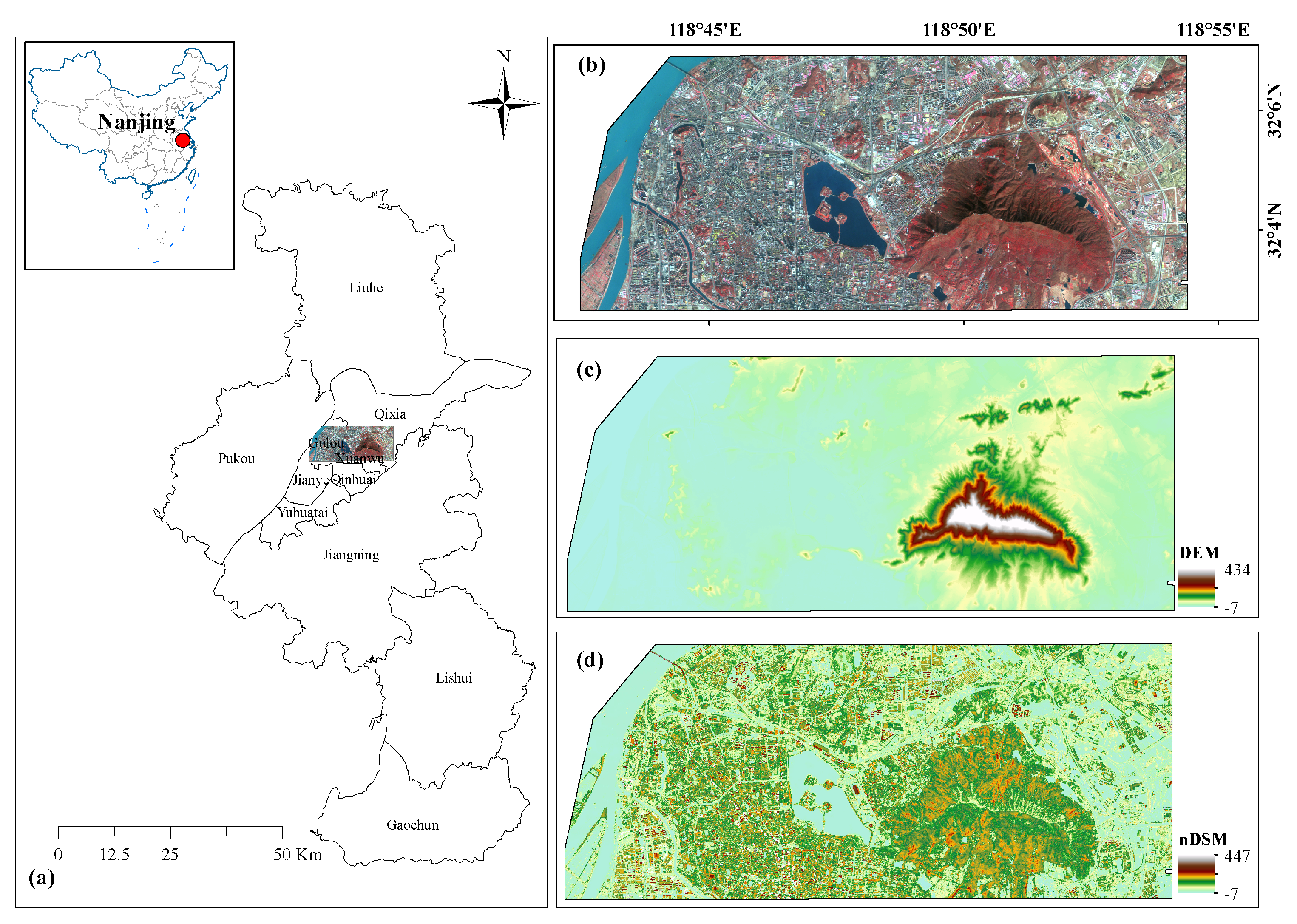
Section 2 describes the study area and presents an overview of datasets as well as the preprocessing. Section 3 reports the methodological details, including feature extraction, classification algorithm, accuracy assessment in conjunction with classification uncertainty. The detailed experimental results are summarized in Section 4. Section 5 provides the discussion and summarizes the paper with remarks and future lines of the research.

2. Study Area and Data

2.1. Study Area

In this work, the study area is located in the central part of the city of Nanjing, China (Figure 1), which is situated on the south bank of the lower reaches of the Yangtze River. It extends approximately 150 km 2 ( 118 42 28 E– 118 54 29 E, 32 2 40 32 7 7 N), with altitude ranging between −7 m and 447 m above mean sea level. The climate of this area belongs to a humid north-subtropical climate with well-defined seasons [38]. The topography is characterized by mountains, hills, plains, and rivers. Rainfall averages 1033 mm per year, occurring mainly in summer. There is a variety of land cover classes in this area, including bare soil, buildings, cropland, grass and woodland (tree and shrub), which makes the study area as a representative test of land cover classification performance for an urban area.

2.2. Data and Pre-Processing

2.2.1. LiDAR Data

Airborne laser scanning data was acquired by Optech ALTM Gemini instrument on 21 April 2009. The wavelength and frequency of the laser pulse were 1.06 μ m and 167 kHz, respectively. The returned laser pulse signals after backscattered from the targets were recorded with the mean point density of 4.1 points/m 2 and up to four returns. The dataset contains point cloud data from a series of overlapping flight lines, each with an overlap of 20–30% between adjacent flight lines. LiDAR data provided accurate height data and contained multiple returns per laser pulse and the intensity information, which reflects the surface characteristics. The identified overlap and noisy points were removed from all LiDAR point clouds. Raster layers for both bare earth surface, digital elevation model (DEM), and the first return, digital surface model (DSM), were generated from a triangular irregular network (TIN) of the LiDAR data points with the pixel size of 10 m. Additionally, by subtracting the DSM with DEM, normalized DSM (nDSM) was created, which represents the height of the above-ground surface features.

2.2.2. SPOT-5 Image

A SPOT-5 multispectral image was acquired over the study area on 1 January 2010. The SPOT-5 data set was composed of shortwave infrared (SWIR) band (1.58–1.75 μ m) with 20m spatial resolution, and three bands with the spatial resolution of 10m covering green (0.50–0.59 μ m), red (0.61–0.68 μ m), and near-infrared (0.78–0.89 μ m). It was orthorectified and resampled to a 10 m pixel size using the software ENVI.
The details of ground reference data is shown in Table 1. We have collected them by using the visual interpretation of the orthorectified SPOT-5, aerial photograph and high-spatial-resolution images from Google Earth (http://earth.google.com/).

3. Methods

3.1. Feature Extraction

3.1.1. Spatial Features

Attribute Profiles (APs), an extension of the Morphological profiles (MPs), were employed to extract spatial features from the SPOT-5 image. APs is a multi-level decomposition of an image with a sequence of morphological attribute filters, which is well suited to modeling the geometrical characteristic instead of the size of the objects [15,39,40]. APs can be formulated as a concatenation of n morphological attribute thinning ( δ C ) and n attribute thickening ( ϕ C ) , obtained by processing the image I according to a criterion T:
A P ( I ) = ϕ k C ( I ) , ϕ k 1 C ( I ) , , ϕ 1 C ( I ) , f , δ 1 C ( I ) , , δ k 1 C ( I ) , δ k C ( I )
Different spatial information, belonging to features present in the nDSM data, can be obtained by APs by many different types of attributes and criterions considered. In this work, two attributes are exploited: area (a) of the regions and standard deviation (s) of the pixels’ grey-level values in the regions. The area can extract information on the scale of the objects, while the standard deviation is associated with the homogeneity of grey-level values of the pixels. In terms of each attribute, the rational values of λ should be selected to initialize each APs. To solve this problem, an automatic scheme is introduced [41]. As far as the λ s is concerned, it is initialized in a way that involves many deviations in the SPOT-5 image data, which can be expressed as follows:
λ s ( I ) = ω 100 σ m i n , σ m i n + ν s , σ m i n + 2 ν s , , σ m a x
where σ m i n , σ m a x and ν s are separately assigned to 2.5, 20.5 and 6, which results in thickening and thinning operations.
The spatial resolution of the SPOT-5 image ought to be considered in adjusting λ a with respect to area attribute, which is mathematically formulated as:
λ a ( I ) = 1000 r a m i n , a m i n + ν a , a m i n + 2 ν a , , a m a x
where a m i n and a m a x are initialized with respective values of 1 and 22 with a step size ν a of 7, and r represents the pixel size of the remote sensing data. Here, all the bands except SWIR band provided by SPOT-5 image were employed to extract spatial features through the APs. As a consequence, a certain number of thickening and thinning operations are acquired for the area attribute.

3.1.2. LiDAR-Derived Features

Given that LiDAR and multispectral can provide complementary information, the LiDAR-based features were extracted to classify land cover except spectral features. The LiDAR feature vector comprises multi-return and intensity LiDAR features, where multi-return LiDAR features can be separate into height-based, return-based LiDAR features. The resulting feature vector f L i D A R can be formulated as follow:
f L i D A R = [ f e l e v a t i o n , f i n t e n s i t y , f r e t u r n ]
(1) Height-based Features
Height information in LiDAR data has demonstrated an importance for the precise description of vertical structure [18,35]. In this regard, height-based LiDAR features were extracted based on 3D points heights within each pixel of 10 m spatial resolution.
In this study, the following height metrics were computed: nDSM, mean, mode, standard deviation, variance, CV (coefficient of variation), skewness, AAD (average absolute deviation), L-moments (L1, L2), L-moment skewness, L-moment kurtosis, MAD median (Median of the absolute deviations from the overall median), MAD mode (Median of the absolute deviations from the overall mode), canopy relief ratio, quadratic mean, cubic mean, and percentile values (1st, 10th, 25th, 50th, 75th, 95th) percentiles.
(2) Intensity-based Features
Given the high separability of spectral reflectance among different materials in the LiDAR sensor’s spectral range (i.e., near-infrared spectral region), intensity, the radiometric component of LiDAR data, can be added as an another feature useful for classifying land cover [26,42]. Intensity variables used in this study were presented: mean, mode, standard deviation, variance, CV, skewness, kurtosis, AAD, L-moments ( l 1 , l 2 ), L-moment CV, L-moment skewness, L-moment kurtosis, and percentile values as with the Height-based features.
(3) Multiple-return Features
Based on the geometry of illuminated surfaces, several types of returns could be achieved in terms of a single pulse emission. However, there is a limited amount of research that has shown the potential use of multiple returns for land cover classification [43]. In this study, the following multiple-return variables were adopted:
  • abovemean: percentage first returns above mean.
  • abovemode: percentage first returns above mode.
  • allabovemean: (all returns above mean height)/(total returns).
  • allabovemode: (all returns above height mode)/(total returns).
  • afabovemean: (all returns above mean height)/(total first returns).
  • afafbovemode: (all returns above mode height)/(total first returns).
Moreover, it should be noted that all the datasets were co-georeferenced and resampled to a 10 m pixel size, which ensures the consistency of corresponding spatial position.
Different feature sets can contribute to improving classification accuracy in a variety of ways. Feature combination can integrate the advantages of different feature sets and has proved to be effective in many projects of urban land cover classification. To gain a detailed understanding of what level of classification result could be obtained by using different scenarios of input features using Random Forest classifier, seven different scenarios were employed for the image classification experiments, as shown in Table 2.

3.2. Random Forests Classifier

3.2.1. Algorithm Principle

Random Forests is a popular ensemble learning approach that has been proved to enhance classification performance significantly and robust to the noise [44,45]. It must be pointed out that Random Forest has been successfully used for land cover mapping using multisource remote sensing data [46].
Random Forests is an ensemble of many classification and regression trees (CARTs) [47]. In training, L CARTs are grown, and each tree is created as follows: (1) bootstrapped samples of the original training set are generated; (2) the tree with no pruning is grown by using the randomly selected feature at each code to do the split. During the classification phase, a new pixel is put down each CART tree, and the output is determined by giving a majority solution over all the trees. As aforementioned, two parameters are needed to be carefully determined: the number of trees ( n t r e e ) and the number of features used for the best split at each node ( m t r y ). In this work, n t r e e is set to be the default value of 500 [46]. m t r y is fixed to the square root of the number of input features.

3.2.2. Feature Importance

Random Forests can generate a quantification of the relative importance of input features, which is of great value for land cover classification using multi-source variables.
The importance of input feature X i can be described as follows. For each tree t of the forest, bootstrapped samples of the training set are applied to the model training, about one-third of the remaining sample set, refer to an out-of-bag (OOB) sample, is used to assess the model performance. Denote by e r r O O B t the error on this O O B t samples. e r r O O B t i is defined as the error, which is computed by using the randomly permuted values of X i in O O B t . The importance of variable of X i can be expressed as:
V I ( X i ) = 1 n t r e e t = 1 n t r e e ( e r r O O B t i e r r O O B t )
where the sum is over all CARTs t of the Random Forests, and n t r e e is the amount of CARTs included in the Random Forests.

3.3. Accuracy Assessment

Ground reference data was divided into training and validation. 5514 reference points were randomly selected for the training, and the remaining 90% reference data were used for the validation. The number of pixels belonging to training and test data is depicted in Table 1. Classification accuracies were summarized based on confusion matrices and derived accuracy metrics. The accuracy metrics consisted of overall accuracy (OA), class-specific accuracy (CA), User’s accuracy (UA) and Producer’s accuracy (PA). The UAs and PAs present information about the commission and omission errors in connection with individual classes, respectively, while the OA represents the percentage of correctly classified pixels. We run 30 times to report the averaged classification accuracies for the purposes of avoiding biased evaluation. In addition, the McNemar z-score was performed to quantitatively measure the differences between different classification scenarios.
The McNemar z-score were conducted by the results generated from only one independent run, whose classification result was closest to the averaged accuracy.

3.4. Classification Uncertainty

Classification uncertainty make the use of the spatial variation of the classifier performance and can be regarded as an advantageous measure to supplement the statistical accuracy metrics from the confusion matrix [48,49]. It should be noted that Random Forests has been employed to provide uncertainty information in the classification of land cover. A significant output of the RF classifier is a probability vector. It contains the class probabilities associated with a pixel x for all classes under consideration: p x = ( p ( 1 ) , p ( 2 ) , , p ( c ) ) , where p ( i ) represents the probability of a pixel being classified into class i, and c is set to be the total number of land cover categories (seven in this study).
Shannon entropy (H) as a quantitative measure of uncertainty can provide the information contained in the probability vector P x , which has been shown the capable of indicating the classifier performance [50]:
H = i = 1 c p ( i ) l o g ( p ( i ) )
The value of entropy H can reach the maximum value 0.85 when all classes have equal probability ( p ( i ) = 1/7), whereas entropy is equal to 0 for a pixel whose maximum probability is 1. The value of uncertainty was scaled to the interval [0, 1] in this study. To acquire the uncertainty values per class, we calculate the median values of entropy H per land cover category.

4. Results

4.1. Classification Results

4.1.1. Classification Using LiDAR Data Alone

First, the classification results of only LiDAR are presented. As shown in Figure 2, the exclusive use of LiDAR-derived height features (Scenario 1 in Table 2) gave rise to the lowest overall classification accuracy 83.17%. The inclusion of intensity information (Scenario 2 in Table 2) increased overall map accuracy to 87.09%, 3.92% higher than Scenario 1. The result of McNemar z-score statistical test suggested the statistically significantly improvement with a 95% confidence level. Another 0.60% improvement was gained with the incorporation of multiple-return features (Scenario 3 in Table 2). In spite of the slight improvement, the result from the McNemar z-score statistical test between Scenario 2 and Scenario 3 indicated that the addition of intensity measures could achieve significantly better classification results.
Table 3 displays the accuracies per class using LiDAR data only. It is apparent that using all input features provided by LiDAR data (Scenario 3) produced better or comparable producer’s and user’s results compared to that of Scenario 1 and Scenario 2. While there are five out of the seven land cover categories were recorded with User’s accuracies higher than 80%, and Producer’s results higher than 80% were produced for four out of the seven land cover classes. The urban land cover classes can be reclassified into three groups. The first group is comprised of classes with high producer’s and user’s accuracies, including building land, cropland, water, and woodland. The second group consists of classes with higher user’s accuracy but lower producer’s accuracy, the grassland class is included. From Table 4, this can be attributable to the fact that grassland was mainly misclassified bare soil and building land. The third group contains the classes with lower producer’s and user’s results, including building land and road. We can take bare soil as an example to explain this phenomenon. The class bare soil was confused by falsely including pixels from cropland and road, resulting in lower user’s accuracy. Bare soil was mainly misclassified as building land and road, thus causing lower producer’s accuracy.
The land cover map produced by using all LiDAR-derived features revealed some problems (Figure 3a). Woodland was misclassified as building land over a large area. Bare soil was not well distinguished from other land cover classes and was primarily misclassified as building land.

4.1.2. Classification Based Only on SPOT-5 Image

We explored the potential of spectral and spatial features derived from the SPOT-5 image for classifying urban land cover classes. The potential of spectral information for classification (Scenario 4 in Table 2) was firstly investigated, leading to an overall classification accuracy of 86.51% (Figure 2). In contrast, the overall classification increased by 6.03% when spatial features were concatenated to spectral measures (Scenario 5 in Table 2). The result of the McNemar z-score statistical test indicated Scenario 5 significantly outperformed the result achieved with dataset Scenario 4 at the 95% level.
Averaged producer’s and user’s accuracies per land cover category with SPOT-5 image only were presented in Table 3. As we can see from the table, producer’s and user’s accuracies with approximate or higher than 90% were recorded for building land, water, and woodland classes by using spectral features only. Producer’s and user’s accuracies were substantially increased when combined with spatial information. The increases were over 10% in all classes except water, which has been well discriminated from other land cover classes. The most noticeable increases in user’s accuracies were for road (24.32%), cropland (17.21%), bare soil (17.09%), and grassland (11.51%). It is interesting to observe that although road class achieved relatively high user’s accuracy, the producer’s accuracy was very low (59.18%). What we can see from the Table 5, class road was mainly misclassified as building land. This confusion may be caused by the fact that class road looks spectrally similar to building land, which makes it very difficult to identify these two land cover classes by using features derived from SPOT-5 image only. Figure 3b shows the classification map derived from the integration of spectral and spatial information. Even though most of the classes were well identified, the road class still has the problem on this map. Many of the road sites were misclassified as building land. This may be in part owing to the reason that there are mixed pixels of building land and road in the urban area.

4.1.3. Classification Results Integrating LiDAR Data with SPOT-5 Image

By combining LiDAR data and SPOT-5 image, five dimensions of input variables are included. To estimate the impact of combinations of SPOT-5 and LiDAR on the classification results, Scenario 6 and Scenario 7 in Table 2 were implemented. It can be seen from Figure 2 that classification accuracy derived from Scenario 6 using all available input features except spatial information was capable of classifying different land cover classes to an overall classification accuracy of 91.96%, which is similar to the classification performance achieved from the best classification using the SPOT-5 image. When the spatial features were combined for classification, all features together provided the maximum ability to separate different land cover classes, resulting in an overall map accuracy of 94.59%, and it is significant at the 95% level as compared to Scenario 6.
Table 6 shows the averaged producer’s and user’s values derived from the combination of SPOT-5 and LiDAR data. When spatial features were employed for classification, the producer’s and user’s results tended to have significant increases for all of the urban land cover categories except already well-discriminated water class. The most noticeable increases were for bare soil (10.49%) and grassland (9.18%), concerning the producer’s accuracy. What stands out in this table is that using all input features together afforded the maximum discriminative power to distinguish land cover types, leading to the highest producer’s and user’s accuracies for almost all land cover classes. As the Table 7 illustrates, although some of the road sites were falsely labeled as building land, higher user’s and producer’s accuracies were obtained compared to the other scenarios of input features.
By a visual inspection of the classification map (Figure 3c) gained by using all input variables, there was a better representation of all land cover classes though there are still some pixels belonging to some road class that is misclassified as building land.

4.2. Feature Importance

4.2.1. Feature Importance for Urban Scenes

Aside from evaluating the influences of different scenarios of input variables on the overall accuracies, an assessment of the relative importance of all input variables was carried out to explore the contribution of each feature to the overall classification accuracy.
By integrating SPOT-5 image with LiDAR data, 102 input variables were contained for each pixel (Scenario 7 in Table 2). To gain insight into the contribution of each input feature, we conduct a feature importance analysis. Figure 4 presented the resulting importance of the 102 variables. From the figure, the nDSM appears the most useful feature in the urban land cover classification. Furthermore, the feature importance scores for the following LiDAR-derived height features were also very high, including variance, cubic mean, 75th percentile value and so on. On the contrary, LiDAR-derived intensity and multiple-return features were found to have little measurable impact on the classification result. Regarding the spectral features derived from a SPOT-5 image, SWIR was the most discriminating. The top 10 most important variable consists of four LiDAR-derived height features (i.e., nDSM, variance, cubic mean, 75th percentiles), SPOT-5 SWIR band and five spatial features.
To evaluate the contribution of each variable to the map accuracy, the number of input variables was subsequently reduced on account of the least importance ranking scores, and the corresponding overall classification accuracy was calculated (Figure 5). From the figure, it can be seen that the overall map accuracies tended to decrease slightly when the first 92 lowest important features were removed. However, the overall accuracies began to fall off rapidly when the remaining 10 most important features are eliminated one by one.

4.2.2. Feature Importance Per Land Cover Class

Figure 6 illustrated the relative importances of all available variables for each land cover class. What we can discover from this figure is that the per-class variable importance varied in a large extent. Regarding the bare soil class (Figure 6a), the most important features involved in height features were nDSM and variance, SPOT-5 SWIR band and some spatial features. However, LiDAR-derived intensity and multiple-return features were not very relevant for the classification of bare soil class. As far as the building land class is concerned (Figure 6b), high values of importances were focused on the elevation and spatial variables. The nDSM belonging to height features exhibited an extremely high value of relevance in terms of the cropland class (Figure 6c). Furthermore, it is worth noting that LiDAR-derived intensity and multiple-return features seemed to be less valuable than other kinds of variables. As for the grassland class (Figure 6d), the features with higher values of importances covered all types of variables except multiple-return features. The feature relevances were more dispersed between height, intensity, spectral and spatial features for road class, which makes the road class more difficult to be distinguished (cf. Table 2). As shown in the (Figure 6f), the SPOT-5 SWIR band played the most important role in discriminating the water class. In addition, some of the height and spatial features also contributed greatly to the classification of the water class due to the higher relative importances. As for the woodland class (Figure 6g), the dominating features concentrated mainly on height and spatial features, among which the most important variables were the spatial features derived from SPOT-5 image.

4.3. Classification Uncertainty

As a complementary metric to the accuracy indices derived from the confusion matrix, classification uncertainty was implemented to provide another indicator to evaluate the classification quality within the acquired urban land cover map, which can be conducive to exploring and spatially locating the superiority of Random Forests with greater detail.
To evaluate the uncertainty of the produced classification maps, median values of the class-specific uncertainties were computed by means of H (Table 8). What is remarkable in this table is that the class-specific uncertainties showed obvious differences with respect to different scenarios of input variables. Results indicated that feature combination can tend to decrease classification uncertainty for different land cover classes, but there is no “one-feature-combination-fits-all” solution. In general terms, relatively high classification uncertainty was obtained for the classification results derived from using LiDAR data alone (i.e., Scenario 1–3). Scenario 7 using all input variables resulted in relatively lower classification uncertainty values for most of the classes when compared to other input features scenarios. The values of median uncertainty (H) differed greatly between the land cover classes in the study area.
Considering the uncertainty values of the land cover class water, all scenarios of input features showed low values of Shannon entropy H equal to 0. One more point we can conclude is that it is not always true that lower uncertainty values correspond to better classification accuracies for all land cover classes. For instance, Scenario 4 and 7 generated similarly low classification uncertainties for road class. However, although the classification uncertainty for class road was the lowest when Scenario 5 was used, road class showed very low classification accuracies in Table 8, which means that class road was misclassified but with little doubt about the final result. A similar result was found with respect to the grassland class. Regarding the woodland class, Scenario 5 and 7 all achieved the lowest value of uncertainty (0.03), corresponding to similar and higher class-specific accuracies. As for the bare soil class, the results on the classification uncertainty presented significant differences among the seven different scenarios of input features. The lowest value of classification uncertainty was obtained by using Scenario 5, but Scenario 5 and 7 all achieved similar and the relatively higher classification accuracy for the bare soil.
The frequency distribution of H was calculated for the incorrect and correct predictions as shown in Figure 7, and the mode of these distributions was discussed. As far as the correctly classified pixels are concerned, a high proportion of pixels were assigned to low values within the [0, 0.1] interval, and fewer correct predictions were associated with an uncertainty H above 0.5. This illustrates that a majority of correctly classified pixels were characterized by lower classification uncertainty, meaning that there was little doubt about the final classification result. Two observations are worth noting. First, correct predictions mostly had low uncertainties, independent of the input feature scenarios. Second, combining SPOT-5 and LiDAR gave rise to a higher proportion of low uncertainties in comparison with the single data alternatives, namely, the integration of SPOT-5 and LiDAR data decreased the uncertainty of classification (Figure 7a). A very large proportion of incorrectly classified pixels yielded the uncertainty values lying within the interval [0.3, 0.9]. This implies that the class decision was uncertain if the mode voted for the incorrect class. Moreover, it was observed that there was a large difference between the seven scenarios of input variables (Figure 7b).
To spatially locate and analyze the merits and deficiencies of the classification results by different input features scenarios, the corresponding classification uncertainty maps were displayed in Figure 8. As the figure shows, distinct patterns in the distribution of classification uncertainty were depicted. It is clear that relatively higher values of Shannon entropy H were observed in the uncertainty map derived from LiDAR data alone, while the uncertainty map derived from Scenario 7 produced lower uncertainty values when compared to the uncertainty maps based on Scenario 3 and Scenario 5, especially for building land. The values of classification uncertainty tended to be higher in the eastern and south-western part of all the classification uncertainty maps, which were located in the peri-urban area. This phenomenon may have resulted from the mixed pixels, containing mixed characteristics from two or more land cover classes. Because of this, it can result in confusion in the process of classification, and assign approximate probabilities to these land cover class, which leads to higher classification uncertainty H.

5. Discussion

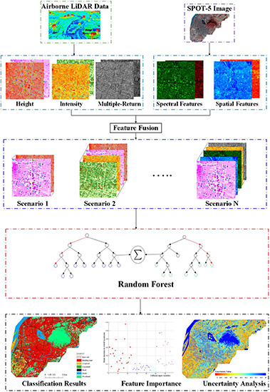
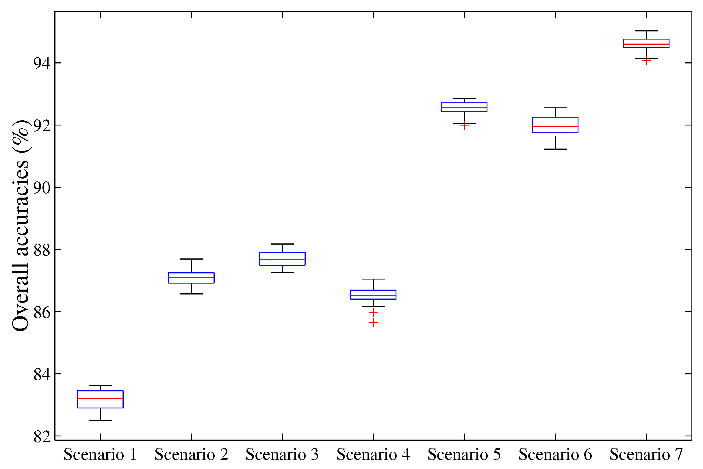
In this work, SPOT-5 and LiDAR data were used to classify different urban land cover classes using Random Forest classifier. We investigated the extent of improvement that various scenarios of input features can bring in classification tasks. Seven feature scenarios were used to incorporate the advantages of different feature sets, which is summarized in 
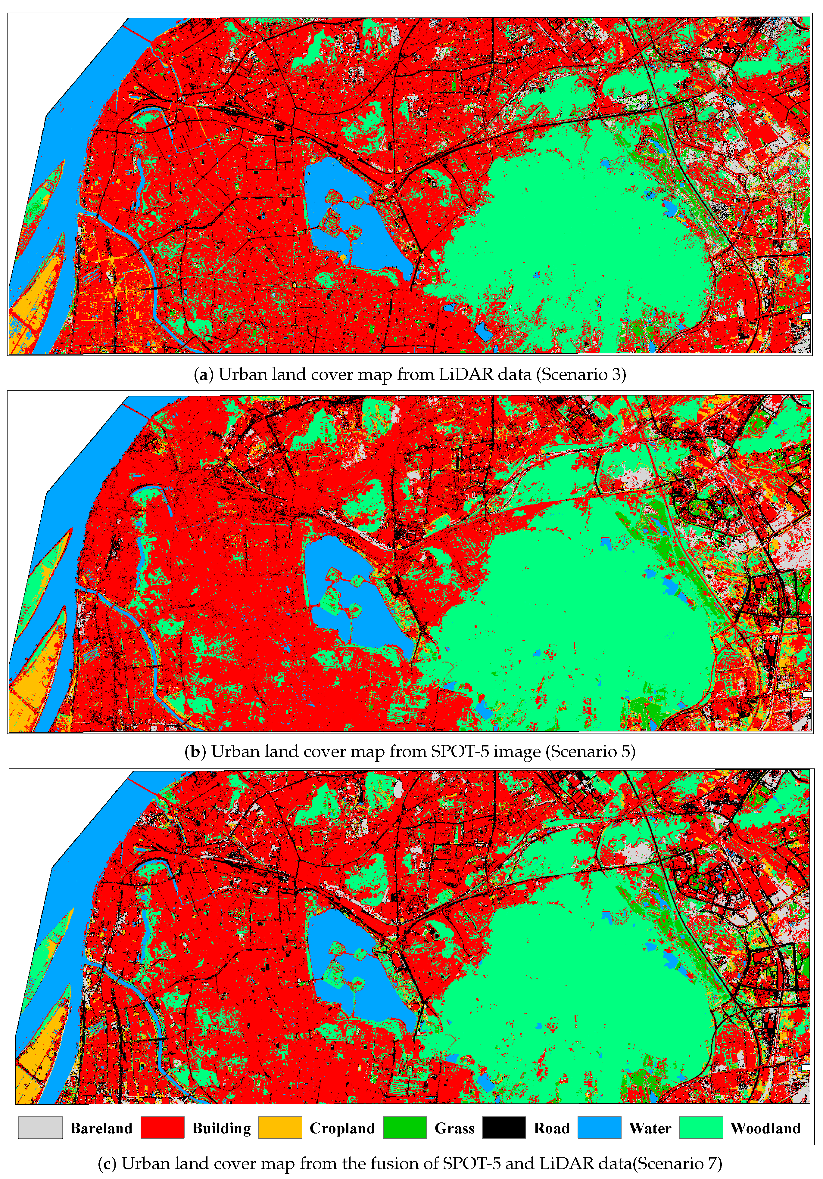
Table 2. When using LiDAR data only, height-based features generated the lowest classification accuracy when compared to other scenarios of input features. The addition of intensity information substantially improved the overall classification accuracy. By adding the return-based features, the overall classification was further improved. When using spectral features alone derived from the SPOT-5 image, the second lowest overall classification accuracy was achieved. The overall map accuracy increased by up to approximately 5% when spatial features were added. It should be noted that by combining SPOT-5 and LiDAR data and using all available features, we obtained the maximum power to discriminate different land cover categories, resulting in the best classification result.
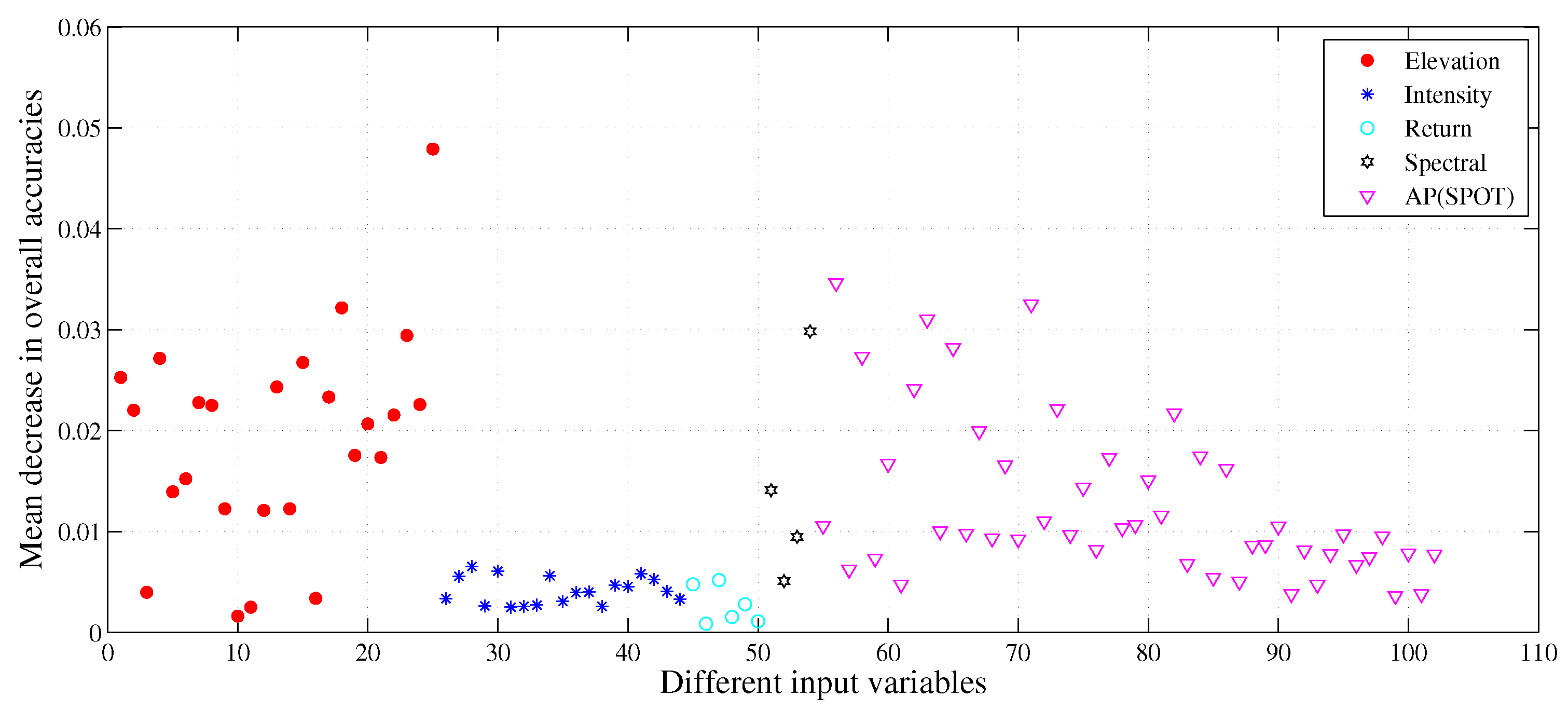
By implementing analysis of the relative importance of all input variables, we can conclude that the nDSM from LiDAR-derived height features appears to be the most important feature in the land cover classification; this is similar to the findings of some previous studies [18,43]. In addition, the feature importance scores for the following LiDAR-derived height features were also high, including variance, cubic mean, 75th percentile value and so on, which means that those LiDAR-derived height features are also of great importance to the urban land cover classification. However, experimental results in this study suggested that LiDAR-derived intensity and return information contributed less to the increment of overall classification accuracy. The SPOT-5 SWIR band is the most beneficial band for the spectral information. On the other side, many spatial features also achieve high feature importance scores. The different input features have different contributions to the overall map accuracy (
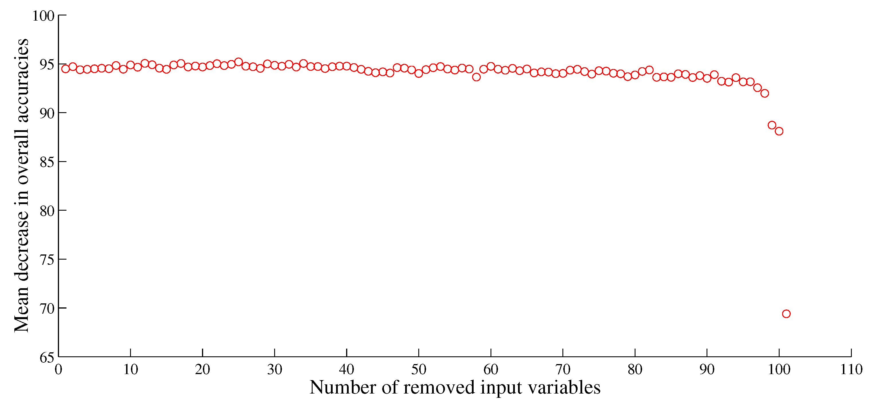
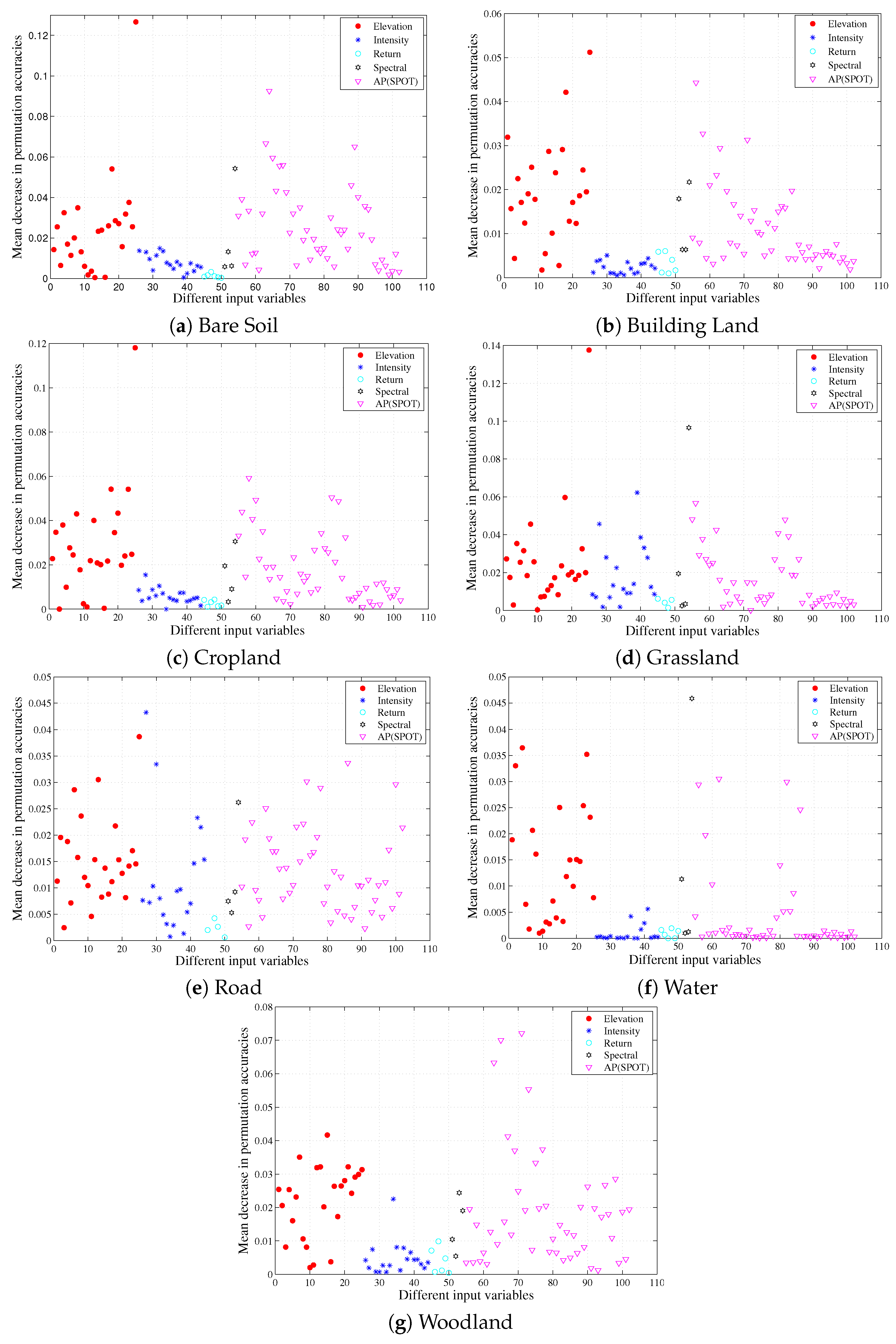
Figure 5). It is not always the case that more input variables ought to generate higher overall classification accuracy. In this study, it has been demonstrated that the overall classification accuracy obtained by using only the 10 most important features is higher than all scenarios of input variables except Scenario 7 using all available input features. Moreover, feature importance per class revealed that the per-class variable importances appeared to be greatly variable.
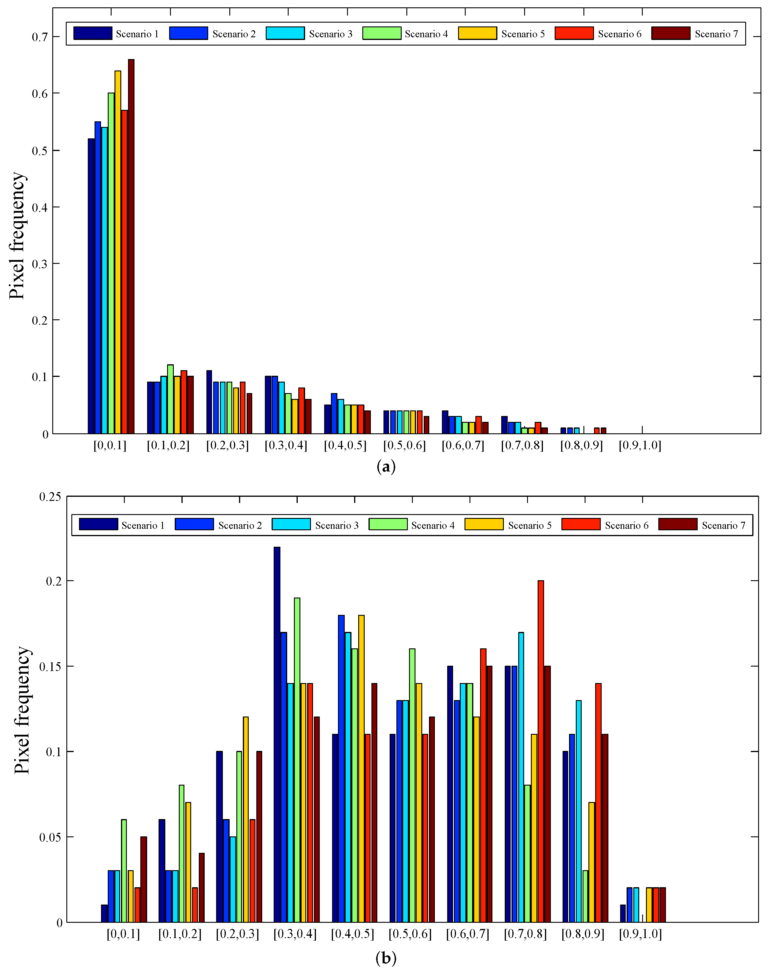
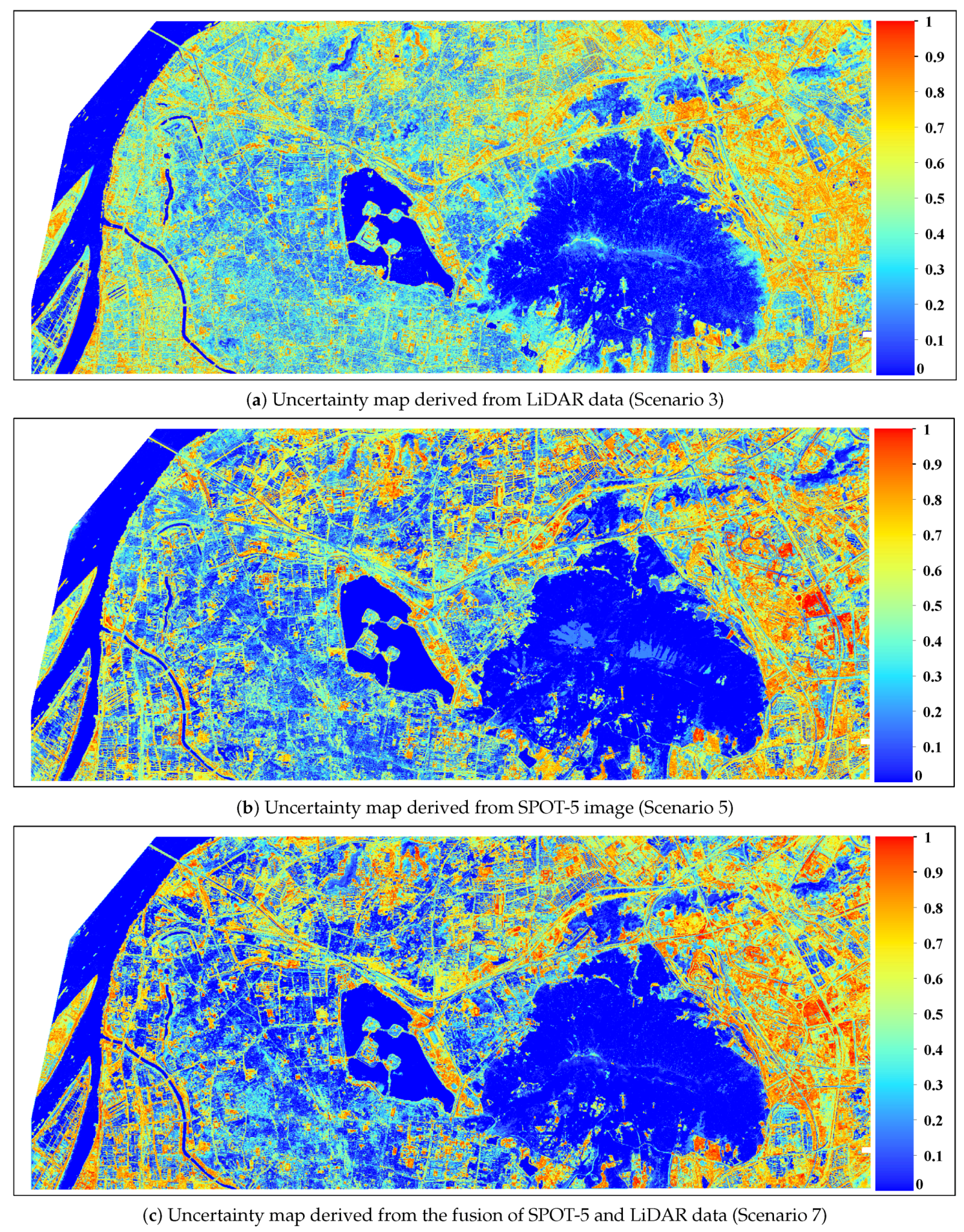
Classification uncertainty analysis can be used as a tool to evaluate the spatial variation of classification performance, and it has been employed in some previous research [48,50]. However, there are very few studies focusing on the impacts of the fusion of multispectral and LiDAR data on the classification uncertainty. The classification uncertainty analysis described in this study are a first step towards the evaluation of classification performance obtained by the fusion of multispectral and LiDAR data. Results of classification uncertainty analysis revealed that feature combination can tend to reduce the classification uncertainty for different land cover classes, but there is no “one-feature-combination-fits-all” solution. The values of uncertainty (H) showed large differences between the land cover classes. It is interesting that the water class has extremely low classification uncertainty, independent of different scenarios of input features. Using all input variables resulted in lower class-specific uncertainties for most of the land cover types as compared to other scenarios of input features. In addition to lower classification uncertainty, all input features can tend to generate a larger proportion of correctly classified pixels with lower uncertainty, which means that there was little doubt about the final decision if the pixel was allocated with correct land cover class. The spatial uncertainty analysis showed that there were higher values of classification in the peri-urban area owing to the effects of mixed pixels.

6. Conclusions

In this work, we explored the use of multi-source remote sensing data to map urban land cover, with a particular focus on available input variables provided by airborne LiDAR and SPOT-5 data. The integration of three feature types (i.e., height, intensity and multiple-return) derived from LiDAR data and multispectral image was firstly used to map the urban land cover. In addition to evaluating the feature importance of all input features for the land cover classification, we firstly explored the impacts of the fusion of multispectral and airborne LiDAR data on the classification uncertainty in this study.
The following findings can be concluded according to the experimental results:
  • We found that the integration of LiDAR and multispectral can provide complementary information and improve the classification performance. The addition of intensity and spatial features are of immense value for improving the classification accuracy. The exclusive use of LiDAR-derived height features produces the land cover map with the lowest map accuracy. The best result is obtained by the combination of SPOT-5 and LiDAR data using all input features.
  • Analysis of feature relevance indicated that LiDAR-derived height features were more conducive to the classification of urban area when compared to LiDAR-derived intensity and multiple-return features. While the nDSM was the most useful feature in improving the classification performance of urban land cover, the feature importance scores for the following LiDAR-derived height features was also very high, including variance, cubic mean, 75th percentile value and so on. Selecting only the 10 most important features can result in higher overall classification accuracy than all scenarios of input variables, except the input feature scenario using all available input features. As for feature importance per class, the variable importance varied to a very large extent.
  • Results of classification uncertainty suggested that feature combination can tend to decrease classification uncertainty for different land cover classes, but there is no “one-feature-combination-
    fits-all” solution. The values of classification uncertainty showed marked differences between the land cover classes. Lower uncertainties were revealed for the water class. Furthermore, using all input variables usually resulted in relatively lower classification uncertainty values for most of the classes when compared to other input features scenarios.
There are some possible developments of this study to be included: (1) to incorporate more beneficial three-dimensional features from LiDAR to further enhance the classification performance; (2) to explore the influence of feature selection on the accuracy and uncertainty of urban land cover classification; (3) to investigate the role of increasing the size of training sets as a possibility to improve the results.

Author Contributions

Jike Chen conceived and designed the experiments; Jike Chen performed the experiments, analyzed the data and wrote the paper. Peijun Du, Junshi Xia, Changshan Wu and Jocelyn Chanussot gave comments, suggestions to the manuscript and checked the writing.

Acknowledgments

This work is supported by National Natural Science Foundation of China (No. 41631176), and the program B for outstanding PhD candidate of Nanjing University (No. 201701B019). We thank Wenquan Han from Nanjing Institute of Surverying, Mapping and Geotechnical Investigation for providing airborne LiDAR data.

Conflicts of Interest

The authors declare no conflict of interest.

References

  1. Cihlar, J. Land cover mapping of large areas from satellites: Status and research priorities. Int. J. Remote Sens. 2000, 21, 1093–1114. [Google Scholar] [CrossRef] [Green Version]
  2. Stefanov, W.L.; Ramsey, M.S.; Christensen, P.R. Monitoring urban land cover change: An expert system approach to land cover classification of semiarid to arid urban centers. Remote Sens. Environ. 2001, 77, 173–185. [Google Scholar] [CrossRef]
  3. Verburg, P.H.; Neumann, K.; Nol, L. Challenges in using land use and land cover data for global change studies. Glob. Chang. Biol. 2011, 17, 974–989. [Google Scholar] [CrossRef] [Green Version]
  4. Friedl, M.A.; McIver, D.K.; Hodges, J.C.; Zhang, X.; Muchoney, D.; Strahler, A.H.; Woodcock, C.E.; Gopal, S.; Schneider, A.; Cooper, A.; et al. Global land cover mapping from MODIS: algorithms and early results. Remote Sens. Environ. 2002, 83, 287–302. [Google Scholar] [CrossRef]
  5. Yuan, F.; Sawaya, K.E.; Loeffelholz, B.C.; Bauer, M.E. Land cover classification and change analysis of the Twin Cities (Minnesota) Metropolitan Area by multitemporal Landsat remote sensing. Remote Sens. Environ. 2005, 98, 317–328. [Google Scholar] [CrossRef]
  6. Baraldi, A.; Parmiggiani, F. Urban Area Classification by Multispectral SPOT Images. IEEE Trans. Geosci. Remote Sens. 1990, 28, 674–680. [Google Scholar] [CrossRef]
  7. Heinl, M.; Walde, J.; Tappeiner, G.; Tappeiner, U. Classifiers vs. input variables-The drivers in image classification for land cover mapping. Int. J. Appl. Earth Obs. Geoinf. 2009, 11, 423–430. [Google Scholar] [CrossRef]
  8. Rogan, J.; Chen, D. Remote sensing technology for mapping and monitoring land-cover and land-use change. Prog. Plan. 2004, 61, 301–325. [Google Scholar] [CrossRef]
  9. Rashed, T.; Jürgens, C. Remote Sensing of Urban and Suburban Areas; Springer Science & Business Media: Berlin/Heidelberg, Germany, 2010; Volume 10. [Google Scholar]
  10. Zhu, Z.; Woodcock, C.E.; Rogan, J.; Kellndorfer, J. Assessment of spectral, polarimetric, temporal, and spatial dimensions for urban and peri-urban land cover classification using Landsat and SAR data. Remote Sens. Environ. 2012, 117, 72–82. [Google Scholar] [CrossRef]
  11. Wurm, M.; Taubenböck, H.; Weigand, M.; Schmitt, A. Slum mapping in polarimetric SAR data using spatial features. Remote Sens. Environ. 2017, 194, 190–204. [Google Scholar] [CrossRef]
  12. Huang, X.; Zhang, L.; Li, P. Classification and extraction of spatial features in urban areas using high-resolution multispectral imagery. IEEE Geosci. Remote Sens. Lett. 2007, 4, 260–264. [Google Scholar] [CrossRef]
  13. Laurin, G.V.; Liesenberg, V.; Chen, Q.; Guerriero, L.; Del Frate, F.; Bartolini, A.; Coomes, D.; Wilebore, B.; Lindsell, J.; Valentini, R. Optical and SAR sensor synergies for forest and land cover mapping in a tropical site in West Africa. Int. J. Appl. Earth Obs. Geoinf. 2013, 21, 7–16. [Google Scholar] [CrossRef]
  14. Benediktsson, J.A.; Pesaresi, M.; Amason, K. Classification and feature extraction for remote sensing images from urban areas based on morphological transformations. IEEE Trans. Geosci. Remote Sens. 2003, 41, 1940–1949. [Google Scholar] [CrossRef] [Green Version]
  15. Dalla Mura, M.; Atli Benediktsson, J.; Waske, B.; Bruzzone, L. Extended profiles with morphological attribute filters for the analysis of hyperspectral data. Int. J. Remote Sens. 2010, 31, 5975–5991. [Google Scholar] [CrossRef]
  16. Pedergnana, M.; Marpu, P.R.; Dalla Mura, M.; Benediktsson, J.A.; Bruzzone, L. Classification of remote sensing optical and LiDAR data using extended attribute profiles. IEEE J. Sel. Top. Signal Process. 2012, 6, 856–865. [Google Scholar] [CrossRef]
  17. Baltsavias, E.P. A comparison between photogrammetry and laser scanning. ISPRS J. Photogramm. Remote Sens. 1999, 54, 83–94. [Google Scholar] [CrossRef]
  18. Yan, W.Y.; Shaker, A.; El-Ashmawy, N. Urban land cover classification using airborne LiDAR data: A review. Remote Sens. Environ. 2015, 158, 295–310. [Google Scholar] [CrossRef]
  19. Amolins, K.; Zhang, Y.; Dare, P. Classification of Lidar Data Using Standard Deviation of Elevation and Characteristic Point Features. In Proceedings of the IEEE International Geoscience and Remote Sensing Symposium, IGARSS 2008, Boston, MA, USA, 7–11 July 2008; Volume 2, pp. II-871–II-874. [Google Scholar]
  20. Xu, S.; Vosselman, G.; Elberink, S.O. Multiple-entity based classification of airborne laser scanning data in urban areas. ISPRS J. Photogramm. Remote Sens. 2014, 88, 1–15. [Google Scholar] [CrossRef]
  21. Guan, H.; Li, J.; Chapman, M.; Deng, F.; Ji, Z.; Yang, X. Integration of orthoimagery and lidar data for object-based urban thematic mapping using random forests. Int. J. Remote Sens. 2013, 34, 5166–5186. [Google Scholar] [CrossRef]
  22. Bork, E.W.; Su, J.G. Integrating LIDAR data and multispectral imagery for enhanced classification of rangeland vegetation: A meta analysis. Remote Sens. Environ. 2007, 111, 11–24. [Google Scholar] [CrossRef]
  23. Hartfield, K.A.; Landau, K.I.; Van Leeuwen, W.J. Fusion of high resolution aerial multispectral and LiDAR data: land cover in the context of urban mosquito habitat. Remote Sens. 2011, 3, 2364–2383. [Google Scholar] [CrossRef]
  24. Yan, W.Y.; Shaker, A.; Habib, A.; Kersting, A.P. Improving classification accuracy of airborne LiDAR intensity data by geometric calibration and radiometric correction. ISPRS J. Photogramm. Remote Sens. 2012, 67, 35–44. [Google Scholar] [CrossRef]
  25. Yan, W.Y.; Shaker, A. Radiometric correction and normalization of airborne LiDAR intensity data for improving land-cover classification. IEEE Trans. Geosci. Remote Sens. 2014, 52, 7658–7673. [Google Scholar]
  26. Song, J.H.; Han, S.H.; Yu, K.; Kim, Y.I. Assessing the possibility of land-cover classification using lidar intensity data. Int. Arch. Photogramm. Remote Sens. Spat. Inf. Sci. 2002, 34, 259–262. [Google Scholar]
  27. Charaniya, A.P.; Manduchi, R.; Lodha, S.K. Supervised parametric classification of aerial lidar data. In Proceedings of the Conference on Computer Vision and Pattern Recognition Workshop, Washington, DC, USA, 27 June–2 July 2004; p. 30. [Google Scholar]
  28. Singh, K.K.; Vogler, J.B.; Shoemaker, D.A.; Meentemeyer, R.K. LiDAR-Landsat data fusion for large-area assessment of urban land cover: Balancing spatial resolution, data volume and mapping accuracy. ISPRS J. Photogramm. Remote Sens. 2012, 74, 110–121. [Google Scholar] [CrossRef]
  29. García, M.; Riaño, D.; Chuvieco, E.; Salas, J.; Danson, F.M. Multispectral and LiDAR data fusion for fuel type mapping using Support Vector Machine and decision rules. Remote Sens. Environ. 2011, 115, 1369–1379. [Google Scholar] [CrossRef]
  30. Guo, L.; Chehata, N.; Mallet, C.; Boukir, S. Relevance of airborne lidar and multispectral image data for urban scene classification using Random Forests. ISPRS J. Photogramm. Remote Sens. 2011, 66, 56–66. [Google Scholar] [CrossRef]
  31. Bigdeli, B.; Samadzadegan, F.; Reinartz, P. Fusion of hyperspectral and LIDAR data using decision template-based fuzzy multiple classifier system. Int. J. Appl. Earth Obs. Geoinf. 2015, 38, 309–320. [Google Scholar] [CrossRef]
  32. Rapinel, S.; Hubert-Moy, L.; Clément, B. Combined use of LiDAR data and multispectral earth observation imagery for wetland habitat mapping. Int. J. Appl. Earth Obs. Geoinf. 2015, 37, 56–64. [Google Scholar] [CrossRef]
  33. Mücher, C.A.; Roupioz, L.; Kramer, H.; Bogers, M.; Jongman, R.H.; Lucas, R.M.; Kosmidou, V.; Petrou, Z.; Manakos, I.; Padoa-Schioppa, E.; et al. Synergy of airborne LiDAR and Worldview-2 satellite imagery for land cover and habitat mapping: A BIO_SOS-EODHaM case study for the Netherlands. Int. J. Appl. Earth Obs. Geoinf. 2015, 37, 48–55. [Google Scholar] [CrossRef]
  34. Reese, H.; Nyström, M.; Nordkvist, K.; Olsson, H. Combining airborne laser scanning data and optical satellite data for classification of alpine vegetation. Int. J. Appl. Earth Obs. Geoinf. 2014, 27, 81–90. [Google Scholar] [CrossRef]
  35. Dalponte, M.; Bruzzone, L.; Gianelle, D. Tree species classification in the Southern Alps based on the fusion of very high geometrical resolution multispectral/hyperspectral images and LiDAR data. Remote Sens. Environ. 2012, 123, 258–270. [Google Scholar] [CrossRef]
  36. Löw, F.; Michel, U.; Dech, S.; Conrad, C. Impact of feature selection on the accuracy and spatial uncertainty of per-field crop classification using support vector machines. ISPRS J. Photogramm. Remote Sens. 2013, 85, 102–119. [Google Scholar] [CrossRef]
  37. Loosvelt, L.; Peters, J.; Skriver, H.; De Baets, B.; Verhoest, N.E. Impact of reducing polarimetric SAR input on the uncertainty of crop classifications based on the random forests algorithm. IEEE Trans. Geosci. Remote Sens. 2012, 50, 4185–4200. [Google Scholar] [CrossRef]
  38. Deng, S.; Katoh, M.; Guan, Q.; Yin, N.; Li, M. Interpretation of forest resources at the individual tree level at Purple Mountain, Nanjing City, China, using WorldView-2 imagery by combining GPS, RS and GIS technologies. Remote Sens. 2013, 6, 87–110. [Google Scholar] [CrossRef]
  39. Dalla Mura, M.; Villa, A.; Benediktsson, J.A.; Chanussot, J.; Bruzzone, L. Classification of hyperspectral images by using extended morphological attribute profiles and independent component analysis. IEEE Geosci. Remote Sens. Lett. 2011, 8, 542–546. [Google Scholar] [CrossRef]
  40. Khodadadzadeh, M.; Li, J.; Prasad, S.; Plaza, A. Fusion of hyperspectral and lidar remote sensing data using multiple feature learning. IEEE J. Sel. Top. Appl. Earth Obs. Remote Sens. 2015, 8, 2971–2983. [Google Scholar] [CrossRef]
  41. Ghamisi, P.; Benediktsson, J.A.; Cavallaro, G.; Plaza, A. Automatic framework for spectral–spatial classification based on supervised feature extraction and morphological attribute profiles. IEEE J. Sel. Top. Appl. Earth Obs. Remote Sens. 2014, 7, 2147–2160. [Google Scholar] [CrossRef]
  42. Zhou, W. An object-based approach for urban land cover classification: integrating LiDAR height and intensity data. IEEE Geosci. Remote Sens. Lett. 2013, 10, 928–931. [Google Scholar] [CrossRef]
  43. Chehata, N.; Guo, L.; Mallet, C. Airborne lidar feature selection for urban classification using random forests. Int. Arch. Photogramm. Remote Sens. Spat. Inf. Sci. 2009, 38, W8. [Google Scholar]
  44. Gislason, P.O.; Benediktsson, J.A.; Sveinsson, J.R. Random forests for land cover classification. Pattern Recognit. Lett. 2006, 27, 294–300. [Google Scholar] [CrossRef]
  45. Du, P.; Samat, A.; Waske, B.; Liu, S.; Li, Z. Random forest and rotation forest for fully polarized SAR image classification using polarimetric and spatial features. ISPRS J. Photogramm. Remote Sens. 2015, 105, 38–53. [Google Scholar] [CrossRef]
  46. Belgiu, M.; Drăguţ, L. Random forest in remote sensing: A review of applications and future directions. ISPRS J. Photogramm. Remote Sens. 2016, 114, 24–31. [Google Scholar] [CrossRef]
  47. Breiman, L. Random forests. Mach. Learn. 2001, 45, 5–32. [Google Scholar] [CrossRef]
  48. Löw, F.; Knöfel, P.; Conrad, C. Analysis of uncertainty in multi-temporal object-based classification. ISPRS J. Photogramm. Remote Sens. 2015, 105, 91–106. [Google Scholar] [CrossRef]
  49. Foody, G.M. Status of land cover classification accuracy assessment. Remote Sens. Environ. 2002, 80, 185–201. [Google Scholar] [CrossRef]
  50. Loosvelt, L.; Peters, J.; Skriver, H.; Lievens, H.; Van Coillie, F.M.; De Baets, B.; Verhoest, N.E. Random Forests as a tool for estimating uncertainty at pixel-level in SAR image classification. Int. J. Appl. Earth Obs. Geoinf. 2012, 19, 173–184. [Google Scholar] [CrossRef]
Figure 1. Maps of the study area are shown as follow: (a) Geographical position of the research area; (b) SPOT-5 multispectral false color composite image acquired on 1 January 2010; (c) Digital elevation model (DEM) and (d) Normalized digital surface model (nDSM).
Remotesensing 10 00872 g001
Figure 2. Overall classification accuracies with different input feature scenarios. The red line inside the box represents the median. The bottom and top of the blue boxes are the first and third quartiles. As for the whiskers, the lowest datum represents the lowest value still within 1.5 IQR (IQR = third quartile—first quartile) of the lower quartile, and the hightest datum represents the highest value still within 1.5 IQR of the upper quartile. Red crosses indicated the outliers.
Remotesensing 10 00872 g002
Figure 3. Classified urban land cover maps generated by Random Forests classifier with different input variables.
Remotesensing 10 00872 g003
Figure 4. Importance of the 102 input features provided by SPOT-5 and LiDAR data.
Remotesensing 10 00872 g004
Figure 5. Overall classification accuracies in the basis of backward exclusion of the least important input variables.
Remotesensing 10 00872 g005
Figure 6. Feature importance per class by using mean decrease permutation accuracy.
Remotesensing 10 00872 g006
Figure 7. Distribution of H for the corrected classified test samples (a) and incorrect predictions (b) as resulted from different scenarios of input features.
Remotesensing 10 00872 g007
Figure 8. Uncertainty maps of the classification results obtained by different scenarios of input variables.
Remotesensing 10 00872 g008
Table 1. Ground Reference in units of pixels for each of the classes.
ClassTraining SamplesTest Samples
Bare soil1131014
Building Land10059043
Cropland1571412
Grassland71638
Road1831646
Water4794306
Woodland5304769
Table 2. Different scenarios involoved in experiments.
Scenario NumberInput VariablesNumber of Features
Scenario 1Elevation25
Scenario 2Elevation, Intensity44
Scenario 3Elevation, Intensity, Multiple-return50
Scenario 4Spectral4
Scenario 5Spectral, AP(SPOT-5)52
Scenario 6LiDAR-derived, Spectral54
Scenario 7LiDAR-derived, Spectral, AP(SPOT-5)102
Table 3. Averaged PA and UA per land cover class achieved from 30 times by using Random Forests classifier. The input scenarios are derived from SPOT-5 and LiDAR data separately.
ClassScenario 1Scenario 2Scenario 3Scenario 4Scenario 5
PA%UA%PA%UA%PA%UA%PA%UA%PA%UA%
BS58.1061.9767.1871.0665.7870.7072.0472.4684.9189.55
BL93.7181.4694.6583.6294.9584.7390.1885.0094.9290.13
CL74.2280.5284.0987.4384.0187.2779.5375.5793.7292.78
GL53.1966.6766.7885.4166.1985.4671.2680.7978.7692.30
RD52.7658.5162.7877.0961.5377.1334.6456.8359.1881.15
WT97.4798.3498.6298.5598.5598.4598.5799.1598.6799.41
WL72.7388.9778.5790.9581.7891.4193.7491.4997.1094.62
OA83.17 ± 0.3087.09 ± 0.2487.69 ± 0.2886.51 ± 0.2892.54 ± 0.20
Note: BS = Bare Soil; BL = Building Land; CL = Cropland; GL = Grassland; RD = Road; WT = Water; WL = Woodland.
Table 4. Example confusion matrix for 7-class urban land cover classification derived from SPOT-5 image and its spatial information using the Random Forests classifier (Scenario 3).
Reference DataTot.UA%
BSBLCLGLRDWTWL
BS6181456485733583174.37
BL144860492964961674410,19284.42
CL3831115914301522130988.54
GL434442680849386.41
RD11999692610291724138374.40
WT523190242518430898.68
WL4726813282443928431291.09
Tot.101490431412638164643064769 22 , 828
PA%60.9595.1582.0866.7762.5298.7282.37 87.68
‡ Total samples; † Overall accuracy (%). Note: BS = Bare Soil; BL = Building Land; CL = Cropland; GL = Grassland; RD = Road; WT = Water; WL = Woodland.
Table 5. Example confusion matrix for 7-class urban land cover classification derived from SPOT-5 image and its spatial information using the Random Forests classifier (Scenario 5).
Reference DataTot.UA%
BSBLCLGLRDWTWL
BS8704818340696789.97
BL908590333365542107955089.95
CL2211302326011137494.76
GL107151930554595.23
RD331897493710117180.02
WT634180142497431598.47
WL3154504210144633490694.44
Tot.101490431412638164643064769 22 , 828
PA%85.8094.9992.2181.3556.9398.6897.15 92.43
‡ Total samples; † Overall accuracy (%). Note: BS = Bare Soil; BL = Building Land; CL = Cropland; GL = Grassland; RD = Road; WT = Water; WL = Woodland.
Table 6. Averaged PA and UA values per land cover class achieved from 30 random trials by using Random Forests classifier. The input feature scenarios derived from the fusion of SPOT-5 and LiDAR data.
ClassScenario 6Scenario 7
PA%UA%PA%UA%
BS75.7179.8386.2089.85
BL97.4689.5597.5292.76
CL87.6790.7193.1295.02
GL70.7989.7479.9794.36
RD68.1984.0573.2791.19
WT99.0599.4899.2399.84
WL90.8795.6996.3795.40
OA91.96 ± 0.3794.59 ± 0.21
Note: BS = Bare Soil; BL = Building Land; CL = Cropland; GL = Grassland; RD = Road; WT = Water; WL = Woodland.
Table 7. Example confusion matrix for 7-class urban land cover classification derived from SPOT-5 image and its spatial information using the Random Forests classifier (Scenario 7).
Reference DataTot.UA%
BSBLCLGLRDWTWL
BS89414822260196592.64
BL738849563439729167960592.13
CL681302232017135895.88
GL3525101001454493.75
RD2744109118303127692.71
WT0100442720427799.88
WL1112234402454567480395.09
Tot.101490431412638164643064769 22 , 828
PA%88.1797.8592.2179.9471.8799.2195.76 94.52
‡ Total samples; † Overall accuracy (%). Note: BS = Bare Soil; BL = Building Land; CL = Cropland; GL = Grassland; RD = Road; WT = Water; WL = Woodland.
Table 8. The values of median uncertainty (H) and class-specific accuracies (CA) for each of the land cover classes achieved by different input feature scenarios. The values of minimum median uncertainty and maximum class-specific accuracies are in boldface.
Scenario NumberBSBLCLGLRDWTWL
HCAHCAHCAHCAHCAHCAHCA
Scenario 10.630.560.290.930.310.750.650.530.620.530.000.980.090.73
Scenario 20.580.680.280.940.210.860.540.650.530.600.000.990.120.78
Scenario 30.600.670.260.950.200.860.520.650.540.610.000.990.120.81
Scenario 40.430.690.210.910.430.810.380.710.370.340.000.980.080.93
Scenario 50.330.850.170.940.220.960.460.840.370.610.000.990.030.97
Scenario 60.580.750.220.970.220.900.550.680.510.690.000.990.090.89
Scenario 70.390.860.130.970.160.950.480.810.380.750.000.990.030.96
Note: BS = Bare Soil; BL = Building Land; CL = Cropland; GL = Grassland; RD = Road; WT = Water; WL = Woodland.

