1. Introduction
In the past decade, lidar-assisted control (LAC) of wind turbines has become an important research topic in the wind energy community [
1]. Whereas traditional wind turbine control systems rely on feedback measurements to control blade pitch, generator torque, and yaw direction, Light Detection and Ranging (lidar) allows preview information about the approaching wind to be used to improve wind turbine control. The shared goal of the various LAC research efforts is to enable a reduction in the levelized cost of energy (LCOE) of wind energy (i.e., the average cost per unit of energy over the lifetime of the turbine, including capital costs, operations and maintenance costs, and all other relevant expenses) through (a) an increase in energy production or (b) a decrease in turbine cost made possible by structural load reduction [
1]. Although several successful field trials have been reported (as discussed in
Section 2.3), LAC is generally still limited to research activities; there remain a variety of obstacles preventing the widespread use of LAC in the wind industry. The objective of this paper is to provide a summary of how lidar systems can be optimized specifically for control applications in order to overcome the barriers preventing the widespread deployment of LAC.
The results presented in this paper are based on the outcome of the IEA Wind Task 32 workshop “Optimizing Lidar Design for Wind Turbine Control Applications” held in Boston, MA in July 2016. IEA Wind Task 32: “Wind Lidar Systems for Wind Energy Deployment” is an international open platform with the objective of bringing together experts from the academic and industrial communities to identify and mitigate barriers to the use of lidar for wind energy applications. During the workshop, participants from academia, national research laboratories, as well as the lidar and wind turbine industries discussed the barriers preventing the widespread use of lidars for wind turbine control, strategies for overcoming those barriers, and ideas for maximizing the effectiveness of lidars for control applications. In this paper, both practical considerations for overcoming the obstacles to the use of lidars for control and theoretical approaches for optimizing lidar scan patterns are discussed.
The remainder of this paper is organized as follows. A review of lidar technology, LAC, and previous work on lidar optimization for control purposes is provided in
Section 2.
Section 3 and
Section 4 discuss the identified practical barriers to the widespread use of lidars for control and strategies for overcoming the barriers, respectively. Theoretical approaches to optimizing lidar scan patterns by minimizing either (a) the error between the lidar measurements and the rotor effective wind speed or (b) the deviation from the intended setpoint of a control variable of interest (e.g., rotor speed) with the use of LAC are described in
Section 5.
Section 6 outlines how a frequency domain model can be used to calculate measurement or controller setpoint error for different scan configurations. Optimal scan parameters are provided for a variety of scan scenarios. In
Section 7, design choices required to maximize the utility of lidar measurements in a feedforward pitch control scenario are illustrated. Time domain simulations show that the rotor speed regulation (or equivalently, generator speed regulation) achieved by an optimized control scenario matches the performance predicted by the frequency domain model. Next, a technology outlook, discussing potential future directions of lidars for control purposes, is provided in
Section 8. Finally,
Section 9 concludes the paper.
2. Background
In this section, a summary of lidar systems developed for control purposes is provided, followed by a brief overview of the different categories of LAC that have been investigated and a discussion of successful field tests that have been reported. The remainder of the section provides a review of the subset of the LAC literature that focuses on lidar optimization for control purposes.
2.1. Lidar Systems for Control Applications
A variety of nacelle lidar systems have been developed for wind turbine control applications, both commercially and for research purposes. The first field demonstration of a nacelle-mounted lidar that is reported in the literature was made in 2003 by Harris et al. [
2], where the authors tested a single-beam continuous wave (CW) lidar mounted atop a utility-scale wind turbine, measuring 200 m upstream of the turbine. CW lidars measure the wind velocity by focusing a laser beam at a specific range and detecting the Doppler shift of the light backscattered from aerosols at the focus point [
3]. Note that, although CW lidars can only measure at a single distance at one time, the focus distance of the lidar can often be adjusted. The technology behind this initial CW lidar [
2] eventually led to the creation of the ZephIR DM nacelle-mounted circularly-scanning CW lidar by ZephIR Lidar (Hollybush, Ledbury, UK). With a configurable focus distance between 10 m and 300 m, the ZephIR DM lidar completes a circular scan containing 50 measurement points once per second [
4]. A similar ZephIR lidar system was placed in the hub, or spinner, of a MW-scale wind turbine, as discussed by Mikkelsen et al. [
5], allowing continuous measurement of the wind inflow without periodic obstruction from blade passage. A more complex spinner-mounted lidar system developed by Sjöholm et al. [
6], also based on a ZephIR, uses two rotating beam-redirecting prisms to scan 400 points per second, roughly evenly distributed over a 100 m-diameter disk, at a preview distance of 100 m, allowing two-dimensional turbulence structures to be examined. In contrast to research-oriented lidar systems relying on complex scan patterns, a nacelle-mounted CW lidar developed by Windar Photonics (Taastrup, Denmark) uses four fixed beam directions to measure the wind 80 m upstream of the turbine [
7]. This simple design is meant to reduce the cost of nacelle lidars for control purposes.
Whereas CW lidars are limited to measuring one point at a time, but are capable of high sampling rates, pulsed lidar systems can measure the wind speed at multiple ranges along the beam simultaneously, but typically require longer sampling periods. Instead of tightly focusing the laser beam at a specific distance, pulsed lidars attribute the backscattered light to different measurement ranges (range gates) according to the elapsed time since the light was emitted by the lidar. Schlipf et al. [
8] used a custom scanning pulsed lidar system based on the Leosphere Windcube V1 lidar to provide preview measurements for lidar-assisted pitch control field tests. The authors configured the lidar to scan a circular trajectory containing six evenly-spaced beam directions with five range gates from 42.7 m (1 rotor diameter (
D)) to 85.3 m (2
D) upstream of the test turbine with a scan period of 1.33 s. Additionally, a five-beam pulsed nacelle lidar has been developed by Avent Lidar Technology (Orsay, France) for control applications. This lidar was used for LAC field field tests performed by Kumar et al. [
9]. The five-beam Avent lidar provides measurements at up to 10 range gates per beam with a maximum range of 300 m and a scan period of approximately 1.25 s [
10]. Note that, while CW lidars can typically measure the wind at a greater number of beam directions per scan than pulsed systems, pulsed lidars have the advantage of being able to measure the wind at multiple ranges per beam direction. Because each range gate corresponds to a different radial distance from the center of the rotor, pulsed lidars are capable of measuring a large portion of the rotor disk area with a small number of beam directions.
2.2. Lidar-Assisted Control Strategies
The study of LAC began in earnest with the 2005 simulation-based investigation of blade pitch control for rotor speed regulation and blade load reduction presented by Harris et al. [
3]. Since then, LAC strategies have been explored using all three main types of wind turbine control actuation: yaw control, generator torque control, and blade pitch control. Furthermore, the use of lidar measurements for control has been investigated for both below-rated operation, particularly for optimizing power capture, as well as operation in above-rated wind speeds, where the objective is to regulate rotor speed and minimize structural loads.
In the below-rated control region, both lidar-assisted yaw control and generator torque control have been investigated. Traditionally, yaw control is performed using wind direction measurements from a nacelle wind vane. However, improper calibration and flow disturbance behind the rotor can produce inaccurate wind vane measurements and rotor misalignment. Field tests performed by Fleming et al. [
11] show that a bias in the wind vane measurements can be detected and removed using measurements from a nacelle lidar, leading to an improvement in energy capture. Scholbrock et al. [
12] discuss yaw control experiments where information from the wind vane is completely replaced by more accurate lidar measurements, similarly resulting in greater energy capture. However, several authors argue that most of the performance increase from full-time lidar-assisted yaw control could likely be achieved by simply removing the wind vane bias, which could be accomplished with a one-time lidar-based wind vane calibration [
11,
13,
14].
During below-rated operation, the primary purpose of generator torque control is to regulate rotor speed. For a subset of the below-rated control region, the objective is traditionally to maintain the tip-speed ratio of the rotor at its optimal value in order to maximize power capture. The use of lidar preview measurements to improve optimal tip-speed ratio regulation via generator torque control has been shown to provide a small increase in energy capture [
13,
14,
15,
16]. However, as observed by Bossanyi et al. [
13] and Schlipf et al. [
16], the large generator torque fluctuations and drivetrain loads that result from this control strategy likely outweigh the modest benefits.
Blade pitch control has been recognized as one of the more promising types of LAC because of the significant rotor speed regulation improvement as well as structural load reduction that can be achieved. Both collective pitch control, requiring estimates of the “rotor effective wind speed” (e.g., rotor average wind speed) [
13,
17,
18], and individual pitch control (IPC), in which each blade is controlled differently to account for spatial variations in the wind field [
13,
19,
20,
21,
22], have been investigated. By mitigating the effect of spatially-varying wind speeds, using lidar measurements of either rotor effective quantities like wind shear or wind speeds local to the individual blades, IPC has the advantage of reducing blade loads as well as non-rotating loads transferred to the drivetrain and turbine structure beyond what can be achieved with collective pitch control. Note that, while most lidar-assisted IPC controller designs only use measurements of the wind
speed variations over the rotor area, Wortmann et al. [
23] have recently proposed a lidar-assisted IPC controller that mitigates the impact of yaw misalignment and vertical inflow in addition to wind shear on blade loads. A subset of lidar-assisted controllers combine pitch control and torque control to optimize the impact of the two types of actuation together [
24,
25,
26,
27], especially during the transition between below-rated operation (primarily torque control) and above-rated operation (primarily pitch control) [
24].
When considering optimal lidar configurations for control applications, it should be noted that LAC applications typically require only a few seconds of preview time, as explained for a variety of lidar-assisted pitch control strategies; Laks et al. [
28] find that a preview time of only 0.2 s is sufficient for reducing blade loads, Bottasso et al. [
26] conclude that only 1 s of preview time is necessary to minimize tower fore-aft loads and generator speed error, and Dunne and Pao [
29] find diminishing returns for generator speed regulation and pitch activity reduction with preview times beyond 2–3 s. As explained by Dunne et al. [
21], less than one second is fundamentally required to overcome the delay from the pitch actuator, while up to a few additional seconds are required to overcome the delay from filtering the lidar measurements to remove unwanted noise.
2.3. Lidar-Assisted Control Field Tests
Despite the large LAC research literature from the past decade, only a small number of field tests have been reported. However, the results of these experiments show that the types of control improvements revealed by theory and simulation can be demonstrated in the field. As mentioned in
Section 2.2, Scholbrock et al. [
12] demonstrated a reduction in yaw error when replacing the wind vane measurements in the yaw controller of the three-bladed 600-kW CART 3 (Controls Advanced Research Turbine), located at the US National Renewable Energy Laboratory (NREL)’s National Wind Technology Center, with wind direction measurements from a nacelle lidar. These yaw control improvements were achieved using the circularly-scanning ZephIR DM CW lidar introduced in
Section 2.1. Several lidar-assisted collective pitch control field tests were performed at NREL’s National Wind Technology Center as well, all using simple feedforward controllers based on wind speed-to-pitch angle lookup tables. In 2012, Schlipf et al. [
8] evaluated a feedforward pitch controller on the 600-kW, two-bladed CART 2 wind turbine using measurements from the custom circularly-scanning pulsed lidar system mentioned in
Section 2.1. During the same year, a similar feedforward controller was tested on the CART 3 turbine using measurements from a BlueScout Optical Control System (OCS) three-beam pulsed lidar, as described by Scholbrock et al. [
30]. Based on these two experiments, Schlipf et al. [
8] report a reduction in rotor speed standard deviation during the above-rated operation when using LAC, while Scholbrock et al. [
30] additionally reveal a decrease in tower fore-aft loads. Kumar et al. [
9] discuss feedforward pitch control experiments on the CART 2 turbine using preview measurements provided by the five-beam pulsed Avent lidar system, described in
Section 2.1 as well. By re-tuning the feedback pitch controller with which the feedforward controller is combined, the authors demonstrated the ability to maintain roughly the same rotor speed error as the original baseline feedback controller allowed, but with significant reductions in tower fatigue loads and pitch activity.
2.4. Lidar System Optimization for Control Applications
Although much of the literature on LAC focuses on controller design rather than the remote sensing aspect, a significant amount of research has been conducted specifically on the optimization of lidar systems for LAC. This section provides a review of existing research on the optimization of lidars for control applications, organized into four categories: (1) lidar optimization via the analysis of controller performance; (2) scan pattern optimization by minimizing measurement error using simulated lidar measurements; (3) scan pattern optimization by minimizing measurement error using computationally efficient frequency domain calculations; and (4) lidar configuration optimization to address practical considerations.
2.4.1. Optimizing Lidars by Assessing Controller Performance
While many lidar-assisted control studies rely on a single lidar scenario for simulations or field testing, some authors have directly analyzed the impact of different lidar configurations on controller performance. In an overview of the benefits of various LAC applications, Bossanyi et al. [
13] arrive at the general conclusion that both pulsed and CW lidars are suitable for control purposes, as long as they can measure roughly 10 points distributed around the rotor area upstream of the turbine every second while providing a few seconds of preview time. They claim that additional measurement points and faster sampling provide diminishing returns, and that a circular scan pattern is nearly as useful as more advanced scan patterns. The lidar model used in this study includes the spatial averaging, or “range weighting”, along the beam that is inherent to both pulsed and CW lidars as well as the limitation to line-of-sight (LOS) velocity measurements (i.e., the projection of the three-dimensional wind vector onto the beam direction). The authors also find that the optimal scan configuration depends on the wind field parameter being estimated; large cone angles are beneficial for measuring wind direction, but harm the accuracy of rotor effective wind speed and wind shear estimates. Finally, the authors suggest that spatial averaging along the beam is helpful for estimating rotor effective wind quantities for control because it resembles the spatial averaging of the wind field by the rotor.
Focusing on a circularly-scanning pulsed lidar, Koerber and Mehendale [
31] discuss the potential for different LAC applications to reduce the cost of energy generated by a wind turbine. The authors investigate the impact of the number of beams (2, 4, 6, or 8) and the number of range gates (1–10) on rotor speed regulation and structural fatigue load reduction for a collective pitch feedforward controller. As expected, the study finds that the controller performance improves as the number of beams and range gates increases, with the largest improvement occurring when moving from two to four beams and diminishing returns beyond eight range gates. Although the authors do not reveal the specific range gate distances, for the maximum 10-range gate scenario, the range gates are roughly evenly spaced so that they span the entire rotor disk area when projected onto the rotor plane. It is concluded that coverage of the rotor plane area is the most important factor for the scan pattern. Finally, the authors show that sampling frequency has little impact on load reduction, as long as it is above 0.5 Hz.
After first analyzing the influence of the scan pattern, spatial averaging, and LOS velocity limitations on overall measurement quality, researchers began to introduce models of wind evolution into LAC simulations. Wind evolution describes the change in turbulent structures as they advect from the measurement location downstream towards the turbine. This represents a deviation from Taylor’s frozen turbulence hypothesis [
32], traditionally assumed during wind turbine simulation, which maintains that turbulent structures remain unchanged while traveling downstream at the mean wind speed. Wind evolution models are typically defined in terms of longitudinal spatial coherence (i.e., the correlation between wind speeds separated by different longitudinal distances as a function of frequency), with low frequency components of the turbulence remaining highly correlated as the wind travels downstream but high frequency components becoming decorrelated due to eddy decay [
33].
Bossanyi [
34] incorporated wind evolution into collective pitch LAC simulations using the theoretical Kristensen wind evolution model [
33], and found that evolving turbulence does not significantly impact the load reduction potential of LAC. Laks et al. similarly included the Kristensen wind evolution model while simulating lidar-assisted IPC for a 600 kW wind turbine. Assuming a hub-mounted CW lidar with three rotating beams, the authors found that blade loads were reduced to nearly the same level as with frozen turbulence for a preview distance of 126 m (∼3
D). At this preview distance, the spatial averaging along the lidar beam was found to effectively filter out the high-frequency structures in the wind that change the most due to wind evolution.
2.4.2. Optimizing Lidars by Assessing the Accuracy of Simulated Lidar Measurements
Another strategy for optimizing lidar scan patterns is the direct comparison between simulated lidar measurements and the true variables they are intended to represent, thereby removing the controller from the analysis entirely. Kragh et al. [
35] examined how accurately different scan patterns are able to measure yaw misalignment (i.e., the relative wind direction) in stochastic turbulent wind fields with a constant yaw error imposed. By modeling a CW lidar with a focus distance of 100 m, the authors compared the accuracy of measurements from a linear scan pattern sweeping left and right at hub height, a circular scan pattern, and a 2D scan pattern that covers more of the rotor disk area, for cone angles of 15
and 30
. Using a 10-min averaging time, it was found that the circular scan results in the lowest error. For all scan patterns, the larger 30
cone angle improves accuracy. However, the authors showed that when horizontal shear is introduced to the wind fields, the accuracy of the wind direction estimates becomes worse; horizontal shear appears similar to yaw misalignment when measurements are constrained to LOS velocities.
Returning to longitudinal wind speed measurements, Simley et al. [
36] simulated measurements from circularly-scanning CW and pulsed lidars rotating at the same speed as the 126 m-diameter rotor of the NREL 5 MW reference turbine model [
37] in stochastic turbulent wind fields. The lidar optimization is made relevant for pitch controlled turbines by analyzing root mean square (RMS) measurement error for the “blade effective wind speed”, approximated by averaging the longitudinal wind speed along a line representing the blade, weighted by the radially-dependent contribution to aerodynamic torque production. A scan radius near 44 m (70% of the rotor radius (
R)) produced the most accurate measurements, in part because the aerodynamic torque production is concentrated near this region of the blade. For the CW lidar model, the optimal preview distance was found to be in the range of 150 to 180 m (1.2 to 1.4
D), depending on the amount of turbulence. Beyond the optimal preview distance, the amount of spatial averaging increases too much (the effective length that is averaged along the beam scales with the square of the focus distance). For shorter preview distances, the cone angle becomes too large and the measured LOS velocities contain too many contributions from the transverse and vertical wind components, instead of the longitudinal component of interest. For the pulsed lidar, however, the measurement error was found to always improve as preview distance increases because the amount of range weighting along the beam remains constant.
Whereas the previous two studies rely on stochastic turbulent wind fields, Simley et al. [
38] simulated lidar measurements using a more physically realistic wind field generated using large-eddy simulation (LES), a computational fluid dynamics (CFD) technique. The LES wind field, with 8 m/s mean wind speed, includes the interaction with a model of an operating NREL 5 MW reference turbine, causing reduced velocities upstream of the rotor in the turbine’s “induction zone”. Wind evolution is also inherently included. Note that wind evolution places an additional penalty on long preview distances due to the decorrelation of the wind. By simulating a hub-mounted 3-beam circularly-scanning CW lidar at (a) the location of the operating turbine and (b) far upstream of the turbine, the impact of the induction zone on measurement quality was investigated. A model-based wind speed estimator, which relies on measured turbine variables to estimate the true wind disturbances, was used to determine the rotor effective wind speed as well as horizontal and vertical shear. With induction zone effects included, the optimal scan radii and preview distances for measuring rotor effective wind speed and shear were found to be 70%
R (44 m) and 60% to 70%
D (76–88 m), respectively. These values are only slightly smaller than the optimal parameters without induction zone effects.
2.4.3. Lidar Optimization Using Frequency Domain Techniques
As an alternative to performing lidar simulations in stochastic or CFD-based wind fields, metrics of lidar measurement quality can often be calculated directly in the frequency domain. This approach is possible because (a) stochastic wind fields are defined by their frequency domain statistics (turbulence power spectra and spatial coherence) and (b) many useful metrics for measurement quality are either directly based on frequency domain definitions, such as the coherence bandwidth, or can be easily calculated using frequency domain information, such as mean square measurement error. Measurement coherence (the correlation between the lidar measurements and the true wind speed at the rotor plane as a function of frequency) can be calculated using a frequency domain wind field model as long as the lidar measurements and true wind speed variables are defined as linear combinations of wind speeds. Because lidar measurements and rotor effective wind speeds can be modeled as weighted averages of the wind speeds along the lidar beam and along the blades or across the rotor plane, respectively, they are well-suited for frequency domain analysis.
There are two main advantages to determining measurement quality directly in the frequency domain rather than based on time domain simulations. First, generating stochastic or CFD-based wind fields and performing time domain lidar simulations is computationally expensive. Second, to arrive at statistically significant measurement quality statistics, results from many different time domain simulations must be averaged together. Frequency domain calculations, on the other hand, only need to be performed once for each lidar configuration and set of wind field parameters, and produce the exact measurement coherence.
Schlipf et al. [
39,
40] combine a simple exponential longitudinal coherence model of wind evolution, introduced by Pielke and Panofsky [
41], with a standard wind field model based on frozen turbulence to form an evolving wind field model. The model is used to calculate the measurement coherence between pulsed lidar measurements and the rotor effective wind speed, defined as the spatial average of the longitudinal wind speeds across the rotor disk. Specifically, the authors calculate the −3 dB cutoff frequency of the transfer function from the lidar measurements to the rotor effective wind speed, describing the bandwidth where the measurements are correlated with the true wind disturbance.
In addition to lidar range weighting and LOS velocity limitations, the frequency domain measurement coherence model used in [
40] includes the effects of sequential scanning (i.e., the use of a single laser to scan across all beam directions in a finite amount of time). In the pulsed lidar measurement model used, the velocity measurements at different range gates are delayed by the amount of time it takes them to reach the first range gate (determined by the mean wind speed according to Taylor’s frozen turbulence hypothesis [
32]). The delayed velocities, which should be roughly in phase with each other, are then averaged together to estimate the rotor effective wind speed. Schlipf et al. [
39] describe the direct frequency domain calculation of lidar measurement coherence as a “semianalytic” approach because spatial averages are approximated using discretization along the lidar beams and across the rotor disk.
Building upon the theory described in [
39], Schlipf et al. [
40] optimize the scan trajectory of a nacelle-mounted circularly-scanning pulsed lidar with five range gates for a wind turbine with a 109 m rotor diameter by maximizing the −3 dB cutoff frequency of the rotor effective wind speed measurement transfer function. Subject to realistic lidar constraints, the cone angle, number of beam directions, the distance of the first range gate, and the spacing between range gates are optimized. Furthermore, the preview time provided by the measurement configuration must be large enough to overcome the time delay resulting from the measurement filter required to remove the uncorrelated high frequencies (discussed in [
39,
42]). Adhering to the constraints, the optimal scan pattern is found to consist of six beam directions along the scan circle (requiring a scan time of 4.8 s) with a cone angle of 21.8
, with the first range gate at 68 m (0.625
D) and a range gate spacing of 13.6 m. This configuration allows the range gates to radially cover almost all of the rotor area. These parameters result in a measurement transfer function cutoff frequency of 0.03 rad/m (which can be converted to a temporal frequency in Hz by multiplying by
, where
U is the mean wind speed). More details about the semianalytic frequency domain model for computing measurement coherence used by Schlipf et al. [
40] can be found in the dissertation of Schlipf [
43].
Simley and Pao [
44] use a frequency domain wind field model similar to that of Schlipf et al. [
40], combining the Kristensen wind evolution model [
33] with a standard wind field definition to semianalytically calculate measurement coherence and other metrics. However, instead of modeling the rotor disk average wind speed, the authors calculate measurement coherence for rotating “blade effective wind speeds”, defined as the average of the longitudinal wind speeds along the length of the blade weighted by the local contribution to aerodynamic torque production. To determine measurement quality, the authors calculate the mean square error (MSE) between the lidar measurements and the blade effective wind speed, assuming an optimal minimum-MSE measurement filter is used (see [
42]). Using the NREL 5 MW reference turbine model, Simley and Pao [
44] optimize the scan parameters of a circularly-scanning hub-mounted CW lidar, finding that the measurement MSE is minimized using a scan radius of 44 m (70%
R) and preview distance of 170 m (1.35
D).
In the dissertation of Simley [
45], the blade effective wind speed model from Simley and Pao [
44] is extended to calculate the “rotor effective” wind speed as well as linear horizontal and vertical shear that result from three rotating blades. The lidar scenario modeled in [
45] consists of a CW lidar with three rotating beams, one for each blade. The measurements from the three beams are used to estimate the rotor effective wind speed and shear components. Wind evolution is included using an empirical exponential coherence formula based on the coherence measured in a variety of LES wind fields [
46]. As described by Simley [
45], for a mean wind speed of 13 m/s and a turbulence intensity (TI) of 10%, the optimal scan radius and preview distance for measuring the rotor effective wind speed for the NREL 5 MW reference turbine are found to be 38 m (60%
R) and 100 m (0.8
D), respectively. The same parameters for measuring horizontal and vertical shear are found to be 44 m (70%
R) and 113 m (0.9
D), respectively. By exploring different wind conditions, Simley [
45] finds that the optimal lidar configuration changes very little as the mean wind speed varies. However, as TI increases, wind evolution becomes more severe, causing the optimal preview distances to become shorter.
2.4.4. Practical Lidar Considerations
Although the frequency domain measurement coherence models discussed in the previous section provide an efficient way to assess the accuracy of different scan patterns, they do not incorporate many practical lidar considerations. Several studies have focused on more practical aspects of lidar optimization, however.
In addition to their assessment of feedforward controller performance for different scan pattern parameters mentioned in
Section 2.4.1, Koerber and Mehendale [
31] discuss the need for high availability and reliability for LAC applications. For a collective pitch feedforward control system relying on measurements from a multiple-beam pulsed lidar system, the authors conclude that the load reduction and rotor speed regulation performance begins to suffer significantly when the availability drops below 50%. Here, availability is defined as the fraction of measurements that are considered acceptable during a given time series, with the majority of the unavailability arising from blockage by passing blades. Given that controller performance is acceptable with 50% availability, the authors suggest that nacelle mounting is a sufficient approach. Note that more specific definitions of availability for control applications, where even a few seconds of measurement unavailability can compromise control performance, are discussed by Davoust et al. [
47]. Using a 5-beam pulsed lidar with 10 range gates, the authors identify the number of valid measurements out of all beam directions and range gates during the previous 3 s as a good indicator of usefulness, concluding that at least 40 valid measurements (out of a maximum of about 130) are needed for reliable control.
Davoust et al. [
48] explore the impact of the scan parameters of a nacelle-mounted Avent pulsed lidar on availability, as well as the relationship between atmospheric conditions and availability. With respect to rotor blockage, the authors explain that one of the most important parameters that determines availability is the fraction of time that a lidar beam direction is unobstructed by a passing blade. This parameter is a function of the diameter of the blade root and the position where the beam intersects the rotor disk. The fraction of time when the lidar beam is unobstructed by the blades increases as the lidar cone angle increases, the height of the lidar above the rotor axis becomes larger, or the position of the lidar behind the rotor plane increases.
Davoust et al. [
48] show that an additional parameter that impacts availability is the ratio between the averaging time used to measure a single LOS velocity and the time it takes for a blade to pass across the lidar beam direction. If this parameter is greater than 1, then the lidar beam will be unobstructed by the blade for part of the signal integration time. As long as the carrier-to-noise ratio (CNR) of the measurement remains above the necessary threshold, a reliable measurement can still be formed. The authors show that lidar availability can be described as a linear combination of the aforementioned geometrical blockage ratio and averaging time ratio parameters, improving as either parameter increases until the averaging time parameter reaches 1. Therefore, availability can be improved not only by adjustments to scan geometry and lidar position, but also by the measurement integration time.
3. Barriers to the Use of Lidar for Control
The following two sections recapitulate the outcome of the group discussions during the IEA Wind Task 32 workshop “Optimizing Lidar Design for Wind Turbine Control Applications”. Furthermore, they summarize the main conclusions of the given presentations where wind turbine manufacturers as well as lidar vendors talked about their perspectives of the requirements and objectives of lidar systems for control purposes. The whole is augmented with the authors` point of view. In general, most of the raised issues are consented by a vast majority, but that does not necessarily represent a consensus of all the workshop participants. Finally, the barriers preventing the widespread use of lidar for control are structured as follows:
3.1. Lack of Clarity in Cost–Benefit Assessment
Based on the current state of the art, it is likely that LAC could contribute to lower LCOE either by (1) an increase in energy production, (2) a decrease in unit costs of a wind turbine by reduction of structural loads, or (3) an extension of the turbines` lifetime, which combines aspects of the aforementioned. However, the question is “how much exactly?”. In particular, the turbine OEMs are interested in assessing the full lifetime costs of the lidar intended to be used for LAC. Besides the initial cost of the device (volume manufacturing already considered), this includes the costs for turbine integration, which consist of mechanical and electrical installation as well as alignment and calibration. Furthermore, all operational costs have to be taken into account. In the end, it all adds up to the need for appropriate cost models for LAC. They should reveal the link between the load reduction potential/increase in energy capture and all relevant aspects of the monetary impact on the wind turbine. Once a break-even point is exceeded, a business case can be established.
3.2. Absence of 100% Availability
It is generally accepted that a lidar device cannot provide uninterrupted measurement data throughout its operating time. Due to the passing of the blades, some portion of the measurements are not suitable for reconstructing the rotor effective wind speed or other wind characteristics. However, even when the lidar is mounted in the spinner, it is nearly impossible to receive 100% availability. Especially on sites with severe atmospheric conditions (clean air, heavy fog), it is challenging to get a high-quality signal all the time. The next difficulty is deciding when the quality should be considered as “good” and how trustworthy the data are. All in all, there is the need to identify a specific metric where the measurement availability can be regarded as acceptable for applicability to LAC actions.
3.3. Risk Assessment and Reliability Issues
On the basis of the preceding section, there are general concerns that come up when implementing LAC on a wind turbine. The question “what happens if there is no or a faulty signal from the lidar?” is ubiquitous among all workshop participants. Understandably, no one would risk harming the turbine or at worst putting people in danger, if the safe operation of the turbine depends on the reliability of the lidar itself. Because of failures in hardware components and/or in software applications, lidars have not always been able to provide service reliably in the past. It is claimed that the technology readiness level (TRL) of currently-available lidar systems for LAC is still too low. As a result, there are not only the aforementioned safety concerns but also the high costs of troubleshooting and repair. Overall, considerations must be made on how long the lidar’s lifetime should be and how it should be designed to require the least maintenance effort.
3.4. Lack of Common Guidelines and Standards
As shown in the previous sections, there is a need for measures to evaluate the performance of a lidar device or of the whole LAC structure. These metrics, such as availability, have to be well defined and all their calculation constraints have to be fully revealed in order to ensure comparability. Another ambiguity is an appropriate threshold for the metrics. Depending on the application, it is not clear how to decide whether an availability value can be considered as “good” or when in terms of LAC an acceptable limit is reached. It would be desirable for all of this information to be provided in common sources to keep all stakeholders aligned. Ideally, a guideline or a standard specifically for LAC would exist.
3.5. Bringing Theoretical Knowhow and Practical Needs into Accordance
It has already been emphasized in
Section 2 that many theoretical aspects of LAC have been covered quite well. Nevertheless, the technology has not advanced beyond prototype field testing on a wide scale yet. Significant long-term tests on multi-megawatt wind turbines have not been reported. On the one hand, this is mainly due to the aforementioned barriers, but it is also because the research community sometimes does not know the mechanisms of the industry as well as the needs of the end users. On the other hand, turbine manufacturers and lidar vendors are often not aware of what is theoretically possible and what is worth trying to implement. In summary, it can be stated that the level of collaboration between different stakeholders still has room to improve.
4. Suggestions for Mitigating the Barriers to the Use of Lidar for Control
The two questions posed during the second part of the workshop’s roundtable discussion were: what are the design suggestions that can mitigate the identified barriers and what are the design suggestions to optimize lidars for control applications, taking into account the identified constraints? The following is an excerpt of the suggestions made by the workshop participants extended by some recommendations by the authors. There is no claim of completeness, neither should the impression arise that work has not already been done in some of the areas. The challenge for the LAC community is to bring all the different aspects together to adequately address the barriers.
4.1. Assess the Cost–Benefit Relationship by Using Methods of Systems Engineering
As mentioned in
Section 3.1, the ultimate goal for LAC is to prove that the technology is able to reduce LCOE significantly. Because LAC is an interdisciplinary field of engineering where technically advanced systems interact with each other, a holistic approach is needed to fully manage complexity. Systems Engineering (SE) methods are designed to combine contributions and balance trade-offs among optimal performance, cost, and schedule while maintaining an acceptable level of risk covering the entire life cycle of a system. Thus, by combining technical and human-centered disciplines like optimization, reliability engineering, and risk management, SE is almost predestined to meet the challenges of LAC. However, there is probably no general answer to the question “how much?”. It is only possible to investigate if turbine
A with lidar
B on site
C is profitable, provided that the most important boundary conditions are known. A key factor for solving these large optimization problems is the existence of cost models for all systems involved. Thus, it is important to get the turbine manufacturers as well as the lidar suppliers involved. On the level of wind turbine optimization, there are already some promising approaches [
49]. The integration of a lidar into the overall system is still missing though. Therefore, a collaboration with “IEA Wind Task 37: Systems Engineering” is highly recommended.
4.2. Improve Measurement Availability with Self-Adjusting Lidars
The mitigation of the availability problem is quite challenging, sometimes impossible. Even the best lidar cannot measure a LOS velocity if there are no aerosols in the air. In the case of finding a threshold when a single measurement can be considered as exploitable for further processing, the key is “adaptivity”. By smartly adjusting e.g., CNR thresholds, sampling periods, lidar data processing parameters depending on wind evolution, or spacings of range gates, a significant increase in availability should be possible. Of course, the lidar should be capable of adjusting “by itself,” without human intervention.
Another way to increase the percentage of availability is by redefinition. In terms of LAC, it would be more functional if rotor effective quantities were used as a metric. Because of averaging effects, it is not necessary for every LOS measurement to be available to calculate these measures and achieve 100% availability. A suitable metric to quantify the overall quality for LAC is the measurement coherence (see also
Section 6.1).
Furthermore, one could address the availability matter by going a step backwards to the site assessment process. When evaluating if several areas are suitable for energy production through wind turbines, the sites could be checked for characteristics that are beneficial for LAC. Besides high aerosol concentration and practically no severe weather conditions, other measures have to be defined to characterize a site as “LAC compliant”. This would probably limit the applicability of LAC to a small proportion of all explored sites, but once a location is found, the likelihood of good availability will be high. Especially for an emerging technology, it is important to reduce risk factors.
4.3. Improve Reliability and Gain Confidence in TRL by Fault Tolerant Control
Even under perfect environmental conditions, it is still possible to get no measurements from the lidar device because of hardware defects or software errors. These reliability issues were discussed a lot amongst the workshop participants. Generally, the more complexity that is added to a system, the more complicated the assurance of keeping technical products highly reliable becomes. A lidar with few but robust components and a manageable amount of features could probably be considered as less error prone. The challenge for the designer is to find a good trade-off between effort, time, and cost in particular. An important aspect to improving reliability in the near term is maintainability. First, it has to be ensured that the maintenance staff of a wind turbine operator is able to perform maintenance work during regular service intervals. Second, the subsystems of a lidar should be designed in a modular way so that they can be quickly replaced as entire units by plug-and play operations in case of a failure.
Finally, let us assume the worst case: a wind turbine is running in LAC mode and suddenly there are faulty measurements or no measurements at all because of availability or reliability problems. In a retrofit scenario for a fatigue load designed wind turbine, there is a simple but effective countermeasure. By switching back to a “normal operation mode”, the wind turbine acts with its standard feedback controller for which it was originally designed. When availability exceeds the specified threshold or the lidar device is put back into operation, the feedforward mode takes over once again. Note that the challenge of smooth switching is still present.
However, the situation is more complicated when the margin of load reduction has already been taken into account during the design of the wind turbine. In that case, a lidar failure would immediately have a negative effect on the turbine’s lifetime and on the safety of the whole system. On a fatigue load designed turbine, one could limit the damage by derating the turbine to a certain percentage of its rated power where the load margins are kept. In the end, it is a matter of the cost–benefit relationship again.
The by far riskiest scenario occurs when LAC is intended to be used in an extreme load driven wind turbine design to detect extreme events and counteract them. Here, even for an LAC compliant site with a self-adjusting highly reliable lidar, there is still some probability that an extreme operating gust could impact and destroy the turbine when the lidar is not in operation. This issue can only be bypassed by adding redundancy to the system.
4.4. Pave the Way towards International Standards
The first step of mitigating the barrier of missing standards has already been taken by publishing this article. This broad summary of lidar optimization for control purposes could serve as a basis for further input from relevant stakeholders. The medium-term goal should be to create a recommended practices document for LAC applications that is to be updated regularly.
Another important aspect regarding standards was revealed during the workshop. The question of how to carry out a type certification for a turbine with LAC came up. To address this question, an IEA Wind Task 32 workshop on the topic took place in Hamburg, Germany in early 2018.
4.5. Strengthen the Collaboration between Academia and Industry
The fact that 33 people attended the workshop clearly shows that there is already a strong motivation from universities (12 participants), national research laboratories (6), wind turbine manufacturers (10) and lidar vendors (5) in such a knowledge sharing event. Researchers and scientists presented their latest findings and representatives from industrial departments reported on their current developments and gave insights into their products and services. Furthermore, it was intended that the different stakeholders would share some of their experience with LAC, including the problems they face. In the future, the challenge for academia will be to summarize and condense its achievements in an easily understandable manner and point out the benefits clearly. To enhance the possibility of creating significant value, the industry should be encouraged to share more of their key knowledge (e.g., cost models)—of course in compliance with non-disclosure agreements between all parties.
4.6. Use a Standardized Simulation Environment in the Early Design Phase
When thinking about the optimization of lidars for control purposes, one should not be limited to the hardware device itself or the implemented software. In fact, there is still a huge potential for improving the preceding simulation process, more precisely the simulation tool chain. The better adjusted these techniques/tools are to the various subtasks of LAC, the more realistic and therefore more reliable the outcomes become. Consequently, establishing a kind of standardized LAC simulation environment would create added value. Furthermore, a modularized process with defined interfaces would ensure that every potential user is not limited to default features. One can optionally swap modules or extend them with needed functions. Wherever possible, new and useful developments should be shared within the community. The following modules are suggested as minimal requirements for a LAC simulation environment:
Pre-Processors: Tools for generating input files for the most common aeroelastic simulation tools (e.g., Bladed, FAST). Furthermore, lidar vendors could share scripts to convert the output data of their specific devices to a defined data format that is compatible with the other modules’ interfaces.
Wind Field Generator: In the context of LAC, wind fields should be generated differently for realistic simulation. Several types of wind events (e.g., extreme operating gusts) have to be included in turbulent wind fields while ensuring acceptable computational effort [
50].
Lidar Simulator: The lidar should be modeled with its most important properties, e.g., number of beams, scanning angles, number and spacing of range gates, update/measurement rate, range weighting function, probe length, etc.
Wind Field Reconstruction: Tools and algorithms for reconstruction of rotor effective wind characteristics from LOS data. A common data format with a defined interface is preferable for immediate application of new lidar devices.
Controller Compilation Framework: Here, the feedback as well as the feedforward controllers and all their subfeatures are included. It is not mandatory to use Matlab/Simulink (The MathWorks, Inc., Natick, MA, USA) like many control engineers, but it is beneficial when source code can be compiled to a dynamic link library (DLL) so the controllers can be shared within the community.
Post-Processing: A wide variety of tools for statistical evaluation and plotting of simulation results.
It is intended that, within one module class, there are several versions that can vary in complexity quite significantly. Depending on the stakeholder’s needs, one can combine the submodules to create user-specific simulation environments. Wherever necessary, modules should also be executable independently to allow focusing on a specific problem.
5. Lidar Scan Pattern Optimization
While ideas for improving lidar availability and reliability, as well as other practical considerations, were presented in
Section 4, this section focuses on the selection of lidar scan locations upstream of the turbine that result in measurements that best represent the actual wind variables of interest that arrive at the turbine. Lidar scan patterns can be optimized for different control strategies (e.g., collective pitch control for rotor speed regulation, IPC for asymmetric rotor load reduction, yaw control), which require measurements of different wind variables (e.g., rotor effective wind speed, wind shear, wind direction). Therefore, there is generally no single scan pattern that is optimal for all control objectives. Because of the great interest in collective pitch feedforward control for rotor speed regulation in the literature, however, the detailed investigations of scan pattern optimization presented in the rest of this paper will focus on measurements of the rotor effective wind speed.
For the purposes of the scan pattern optimization discussed here and in
Section 6, rotor effective wind speed is defined as the time-varying mean value of the longitudinal
u components of the wind over the rotor disk area. For simplicity, it is assumed that (1) all locations in the rotor disk have equal importance; (2) the response of the rotor is purely a function of the linear combination of wind speeds across the rotor disk; and (3) the transverse
v and vertical
w wind components can be neglected. Perfect alignment between the rotor and the mean wind direction is assumed (i.e., no yaw misalignment or vertical inflow angle).
The scan pattern optimization performed here is subject to the following potential sources of measurement error: (1) the evolution of the wind as it travels from the measurement location to the rotor plane; (2) the limitation to LOS measurements (i.e., the “corruption” of the wind speed measurements by the
v and
w components of the wind, when the
u component of the wind is of interest); (3) range weighting, or the spatial averaging of the wind speeds along the beam direction; and (4) the fact that a scan pattern containing a finite number of points will not perfectly resemble a rotor disk average. All scan patterns are optimized for a rotor diameter of
D = 126 m, the rotor diameter of the NREL 5 MW reference turbine [
37].
5.1. Metrics for Assessing Measurement Quality
To compare the effectiveness of different scan patterns, an appropriate metric representing lidar measurement quality must be defined. One simple metric that describes measurement accuracy is the MSE between the true rotor effective wind speed at the turbine
and its estimated value based on the lidar measurement
:
However, because lidar-based estimates of the rotor effective wind speed are not perfectly correlated with the wind at the rotor due to wind evolution and other sources of measurement error, it is beneficial to low-pass filter the measurements before they are used by the controller. As will be described in the next section, an optimal filter
can be derived that minimizes the measurement MSE. Therefore, a useful metric for determining measurement accuracy is the MSE between the true rotor effective wind speed and its optimally-filtered lidar-based estimate:
Metrics describing measurement quality can be made more meaningful by including the response of the turbine to the wind inflow, instead of concentrating on the wind variables alone. For example, the impact of the wind inflow on a turbine variable of interest
, when the imperfect measurement
is used as input to the feedforward controller, can be used to judge measurement quality. Assuming the objective of the lidar-assisted controller is to minimize the magnitude of a wind turbine variable, the variance of
is an appropriate measurement quality metric. Specifically, for the control objective of minimizing the mean square error between the generator speed
and the rated generator speed
, this metric becomes:
Finally, measurement quality can be judged by the highest frequency at which the measurement remains correlated with the true rotor effective wind speed. In this case, the objective of the scan pattern optimization is to maximize the correlation bandwidth, allowing the feedforward controller to mitigate the impact of as much of the frequency content of the wind as possible. The correlation between the rotor effective wind speed
and its lidar-based estimate
as a function of frequency is described by the magnitude-squared coherence between the two signals:
. The magnitude-squared coherence between two signals
a and
b is defined as
where
is the cross-power spectral density (CPSD) between signals
a and
b,
is the power spectral density (PSD) of
a, and
is the PSD of
b. Values of coherence range from 0 to 1, where a value of 0 indicates that the two signals are completely uncorrelated while a value of 1 indicates perfect correlation. A reasonable value of coherence for representing the boundary between frequency components that are uncorrelated and correlated is 0.5 [
51]. Therefore, a useful metric for indicating measurement quality is the frequency at which the measurement coherence crosses below 0.5:
5.2. Lidar System Configurations
The coordinate system and basic parameters used to describe the scan patterns analyzed in this paper are shown in
Figure 1. A scan pattern may contain many different measurement points, but each point can be defined by its upstream preview distance
d from the lidar unit in the
direction, its radial distance
r in the
plane from the point
d m directly upstream of the lidar unit, and the azimuth angle
in the
plane, where
= 0 indicates a measurement at the top of the scan circle defined by
d and
r. The measurement points can be equivalently described by their measurement distance
F and cone angle
. For simplicity, it is assumed that the lidar is located at the origin, which is defined as the rotor hub position.
Both CW and pulsed lidars are examined here when analyzing scan patterns. Measurements from both types of lidars consist of wind speeds spatially averaged along the beam direction. However, the range weighting functions, which describe how heavily wind speeds at different radial distances are weighted, are different. The range weighting function for a CW lidar changes as the focus distance of the lidar increases; the full-width-at-half-maximum width of the weighting function is proportional to the square of the focus distance. Therefore, the farther a CW lidar is focused, the more spatial averaging occurs. The range weighting functions for pulsed lidars remain approximately constant regardless of the range gate distance.
Figure 2 shows theoretical range weighting functions for a CW lidar with focus distances of 50 m, 100 m, and 150 m as well as for a pulsed lidar (shown without loss of generality at a measurement distance of 100 m), with parameters roughly based on the ZephIR 300 CW lidar [
52,
53] and the WindCube WLS7 pulsed lidar [
53,
54], respectively. More information about the range weighting functions can be found in Simley et al. [
36].
Several types of scan patterns are investigated in this paper for CW and pulsed lidars, all roughly based on lidar systems that have been developed commercially. The measurement quality achieved by each scan pattern is compared to a single point measurement upstream of the turbine at hub height, representing the most basic measurement scenario, as well as the longitudinal wind speed averaged over the rotor disk area upstream of the turbine, acting as an “ideal” preview measurement of the rotor effective wind speed. A preview distance of 50 m is used for the single-point and ideal measurements to match the closest range gate available for pulsed lidar measurements in this analysis.
After the point measurement, the simplest lidar scan pattern investigated is the two-beam lidar, with both beams measuring at hub height. This configuration is analyzed for a CW lidar, as shown in
Figure 3b, and a pulsed lidar, illustrated in
Figure 3c. Note that all pulsed lidar scan patterns modeled in this paper contain 10 evenly spaced range gates beginning at a range of 50 m and ending at the farthest range (no more than 300 m), parameters achievable with the Avent lidar system [
9,
10]. The next level of complexity is represented by a four-beam lidar, with CW and pulsed configurations shown in
Figure 3d,e, respectively, based on the Windar lidar [
7] and the four-beam version of the Avent system [
10]. For the four-beam configuration, the beams are oriented at azimuth angles of
=45, 135, 225, and 315 degrees. The last realistic scan pattern investigated is the circular scan consisting of 50 points evenly spaced around a scan circle, based on the ZephIR DM lidar system [
4], shown in
Figure 3f. Because pulsed lidars typically require longer sampling times than CW lidars, only the CW configuration is analyzed for the circular scan scenario due to the high sampling rate required to complete the scan in a reasonable amount of time relative to the lidar preview time.
All of the commercial lidars that these scan patterns are inspired by can complete a full scan in approximately 1 s. Because of the relatively short scan times compared to typical feedforward control time scales, the calculations of measurement quality are simplified in this investigation by assuming each point in the scan pattern is measured simultaneously. Each of the scan patterns shown in
Figure 3 is optimized by varying the preview distance
d and scan radius
r of the scan (or, equivalently, the measurement distance
F and cone angle
). For the pulsed lidar configurations, the 10 range gates measured are evenly spaced between 50 m and the maximum range given by the measurement distance parameter
.
5.3. Lidar-Based Wind Parameter Estimation
Line-of-sight velocity measurements from a lidar can be described as the opposite of the dot product between the unit vector in the direction that the beam is oriented (
) and the wind speed vector at the measurement point (
):
Note that the true velocity measured by a lidar is a spatial average of the LOS velocities along the lidar beam, modeled as the integral of the LOS velocities along the beam weighted by the range weighting function. For control purposes, wind parameters such as the rotor average wind speed, wind shear, and wind direction are more useful than the LOS velocities provided directly by a lidar. Therefore, the wind parameters of interest must be estimated from the LOS velocities.
To estimate the wind parameters, an appropriate wind field model must first be defined. In general, it is not possible to distinguish between horizontal wind direction and horizontal shear (or vertical inflow angle and vertical shear) using LOS velocity measurements from a lidar scan pattern. Consequently, the two most common wind field models used for wind parameter estimation consist of (a) uniform wind speed across the rotor including horizontal and vertical wind direction, and (b) no transverse or vertical wind speeds, but linear horizontal and vertical shear [
55].
Regardless of which wind field model is assumed, for a scan pattern with N unique beam directions, , the solution for the estimate of the rotor average wind speed perpendicular to the rotor, used for optimizing CW lidars in this paper, is given by
However, for pulsed lidars, measurements at different range gates can be combined more effectively by delaying the measured velocity signals at each scan point by the estimated amount of time it takes the wind to travel to the plane where the closest range gate is located, according to Taylor’s frozen turbulence hypothesis [
32]. This effectively “stacks” the measurements from different range gates together before averaging by removing their relative time shifts (although the farther a range gate is from the rotor plane, the more the measurements will suffer from wind evolution). For pulsed lidars, an estimate of the rotor average wind speed, which is used for scan pattern optimization in this paper, can therefore be expressed as
where
is the longitudinal position of measurement point
i,
is the longitudinal position of the range gate closest to the rotor, and
U is the mean rotor effective wind speed. Note that, in practice, the estimation of the rotor effective wind speed could be improved by delaying measurements at the different range gates according to their height-dependent mean wind speed, accounting for wind shear. In this work, however, it is assumed that the wind advection speed is the same at all heights.
More information about wind parameter estimation using lidar measurements, including a discussion of nonlinear methods for estimating all five wind parameters described in this section simultaneously, can be found in Raach et al. [
55].
6. Frequency Domain Optimization
This section begins with a discussion about how the lidar measurement quality metrics introduced in
Section 5.1 can be directly computed via frequency domain calculations using a frequency domain wind field model. Next, the frequency domain calculation procedures are used to optimize the parameters for the scan patterns presented in
Section 5.2 for each measurement quality metric.
6.1. Frequency Domain Calculations for Assessing Measurement Quality
Because lidar measurements and the rotor effective wind speed can be modeled as linear combinations of the wind speeds at different points in space, it is relatively straightforward to compute the measurement quality metrics in
Section 5.1 using a frequency domain wind field model containing the power spectral densities (PSDs) of the three wind speed components and the spatial coherence between wind speeds at different points. As discussed in
Section 2.4.3, direct frequency domain calculations of the metrics describing measurement quality are much more computationally efficient than calculations based on simulated lidar measurements and wind speeds.
The wind field model used here consists of the Kaimal turbulence spectrum and the spatial coherence model described in the International Standard IEC 61400-1 Ed. 3 [
56]. Whereas the IEC standard only describes spatial coherence for the transverse
y and vertical
z directions, wind evolution is modeled here using the empirical longitudinal coherence formula based on LES data developed by Simley and Pao [
46]. Note that the theoretical longitudinal spatial coherence model described by Kristensen [
33] is often used as well. The spatial coherence model defined in the IEC standard [
56] is modified further by extending the transverse and vertical spatial coherence formula used for the
u component of the wind to the
v and
w components as well (the IEC standard defines the
v and
w components as having zero spatial correlation, but this could lead to unrealistically low error from LOS limitations).
Although
Section 5.1 describes the possibility of assessing measurement quality using the raw lidar measurement MSE (Equation (
1)), it is more appropriate to filter the lidar measurements to remove unwanted noise before using them in the controller (Equation (
2)) [
42]. Therefore, the following three metrics introduced in
Section 5.1 will be used for scan pattern optimization in this section: (1) mean square measurement error with optimal filtering; (2) generator speed variance resulting from combined feedback-feedforward control with optimally filtered lidar measurements; and (3) the 0.5 measurement coherence bandwidth. As explained in Schlipf et al. [
39] and Simley and Pao [
42], the optimal filter that minimizes the MSE between the lidar measurement and the true rotor effective wind speed is given by the transfer function
where
is the CPSD between the rotor effective wind speed and its lidar-based estimate and
is the PSD of the lidar measurement.
The simplest measurement quality metric to calculate is the correlation bandwidth, based on the measurement coherence:
. As derived by Simley and Pao [
42], the measurement MSE using the optimal filter from Equation (
9) can be calculated by integrating over the PSD of the measurement error:
where
is the PSD of the true rotor effective wind speed.
Additionally, as shown by Simley and Pao [
42], the generator speed MSE (letting
simply represent the deviation from the generator speed setpoint) resulting from the use of combined feedback-feedforward control with optimally-filtered lidar measurements can be expressed as
where
is the closed-loop transfer function from rotor effective wind speed to generator speed error. Equation (
11) uses the assumption that the feedforward controller is designed to perfectly cancel the impact of the wind speed disturbance on the generator speed, as long as perfect preview information is provided. Following the pitch controller tuning recommendations in Hansen et al. [
57], the closed-loop transfer function
used in this paper is chosen to have a second order response with natural frequency
= 0.6 rad/s and damping ratio
= 0.65. More information about the combined feedback-feedforward controller is provided in
Section 7.1.
Detailed descriptions of how the PSDs
and
as well as the CPSD
, used to compute all of the performance metrics discussed here, can be calculated from a frequency domain wind field model using Fourier properties are available in Schlipf et al. [
40] and Simley [
45].
6.2. Detailed Optimization Example: Circular Scan Pattern
All measurement quality calculations are performed for a wind field with mean wind speed
U = 13 m/s (1.6 m/s above rated wind speed for the NREL 5 MW reference turbine) and IEC Class B normal turbulence model turbulence intensity [
56].
Figure 4 reveals how the coherence bandwidth, optimally-filtered measurement MSE, and generator speed MSE with optimally filtered preview measurements depend on the scan radius and preview distance for the circular-scanning CW lidar scenario. The optimal scan radii that maximize the coherence bandwidth and minimize measurement MSE as well as generator speed variance are all around 40 m (∼0.65
R) indicating that measurements at this radius yield the best approximation to a rotor disk average. Although the optimal preview distances are different for the three metrics (∼70–90 m), they reveal the same general trend. Measurements closer to the rotor than the optimal preview distance, resulting in larger cone angles, suffer from LOS velocities that contain too many contributions from the transverse and vertical wind speeds. Measuring the wind farther away than the optimal preview distances causes wind evolution to become more severe, increasing measurement error as well. Note that the measurement quality is more sensitive to deviations in scan radius from the optimal point than to different preview distances. The specific optimal scan parameters for the different measurement quality metrics in
Figure 4 depend on which frequencies are weighted most heavily in the particular metric.
6.3. Scan Pattern Optimization Results
For the seven lidar scan scenarios provided in
Figure 3, the maximum achievable coherence bandwidth along with the minimum achievable measurement MSE and generator speed MSE corresponding to the optimal scan parameters with optimal filtering are compared in
Figure 5. The provided measurement MSE values are normalized by the variance of the rotor effective wind speed, whereas the generator speed MSE values are normalized by the generator speed variance with feedback control only. All three measurement quality metrics reveal the same trends: (1) as the number of beams increases, the measurement accuracy increases as well and (2) for the same number of beams, the additional measurement ranges afforded by pulsed lidars improve measurement accuracy compared to a CW lidar. All lidar measurement scenarios improve upon a single point measurement of the wind speed at hub height. However, the measurement accuracy is much higher for the ideal rotor disk average wind speed measurements than for any realistic lidar scenario. Here, the only source of measurement error is wind evolution due to the 50 m preview distance between the measurement plane and the rotor disk.
The optimal coherence bandwidth, measurement MSE, and generator speed MSE values shown in
Figure 5 for the seven lidar measurement scenarios are listed in
Table 1, along with the scan parameters required to achieve them. For the two pulsed lidar scenarios, the scan radius
r, preview distance
d, and focus distance
F indicate the values corresponding to the farthest range gate measured.
Table 1 reveals that the optimal scan parameters depend on the measurement quality metric that is being optimized. Note that the optimal scan parameters for maximizing coherence bandwidth and minimizing generator speed MSE are almost always the same. However, the optimal scan radius and preview distance values that minimize measurement MSE are typically greater than they are for the other two metrics.
The reasons why the optimal scan parameters that maximize coherence bandwidth or minimize generator speed MSE are shorter than for minimizing measurement MSE are related to the frequencies that are weighted most heavily when calculating each metric (see Equations (
10) and (
11)). For example, due to the frequency response of the closed-loop transfer function
, the generator speed MSE is most sensitive to measurement error in the frequency band near 0.05 Hz, while the measurement MSE is more sensitive to measurement error at lower frequencies, where more of the energy in the wind is concentrated. This explains why generator speed MSE is minimized (and coherence bandwidth is maximized) using shorter preview distances, which prevent the coherence at higher frequencies from decaying too much from wind evolution. When minimizing measurement MSE, on the other hand, it is more important to measure farther away, thereby reducing LOS errors, which affect the low frequencies as much as the high frequencies.
Measuring farther away from the turbine adds the benefit of more volume averaging along the lidar beam due to the wider range weighting function for CW lidars. Longer preview distances also permit larger scan radii to be achieved with smaller cone angles, allowing greater radial coverage of the rotor disk area while reducing LOS errors. The additional volume averaging and greater rotor disk coverage help approximate the rotor effective wind speed, further explaining why longer preview distances and larger scan radii are optimal for minimizing MSE, where additional wind evolution at high frequencies can be tolerated.
It should be noted that the optimal scan radius and preview distance parameters listed in
Table 1 are specific to a 126 m-rotor diameter turbine. However, when expressed in non-dimensional units of rotor diameters and rotor radii, the optimal scan parameters roughly translate to different rotor sizes. Furthermore, the optimal scan parameters presented in this section are only valid for measurements of rotor effective wind speed; when measuring other wind variables such as shear or wind direction, the optimal parameters are typically different. For example, as discussed by Simley [
45], measurements of horizontal and vertical wind shear are more accurate with larger scan radii. Additionally, as presented by Kragh et al. [
35], measurements of wind direction tend to improve with larger cone angles. Finally, the presence of yaw misalignment or vertical inflow may change the optimal scan parameters, likely favoring shorter preview distances so that the measured wind is more representative of what hits the rotor.
While this section presented a method for optimizing lidar scan patterns for measurement accuracy, it should be noted that in practice there may be other objectives that are as important or even more important than minimizing measurement error. For example, the load reduction offered by the lidar-assisted controller is likely a more useful metric for comparing different lidar scan patterns, although it is harder to calculate using frequency domain techniques. Additionally, the extra preview time provided by longer preview distances may be useful when attempting to detect extreme wind events and take necessary actions to protect the turbine. Finally, measuring the wind at multiple range gates with a pulsed lidar offers the advantage of being able to track wind speeds as they travel towards the turbine as well as allowing measurements at different preview distances to be combined to improve the simultaneous estimation of wind shear and direction, as described by Raach et al. [
55].
7. Time Domain Optimization
In the two previous sections, the question of how lidar scan patterns can be optimized for control has been addressed using a few different metrics. This section now deals with the question “how can the lidar data processing and feedforward controller be optimized to improve the performance of wind turbine control?”. To provide a basic understanding of LAC, the section focuses on the following two aspects:
Filtering: Measurement filtering is crucial. No filtering or insufficient filtering of uncorrelated frequencies will cause unnecessary control actions, which will likely result in increased loads. By filtering out correlated frequencies, however, possible benefits of LAC algorithms will not reach their full potential.
Timing: Temporal information about the inflowing wind field is necessary for control purposes. Because this information is available ahead in time, the lidar-assisted control action needs to be synchronized with the disturbance impact on the rotor.
The remainder of the section is organized as follows:
Section 7.1 provides the basic background to understand the main objectives of the section. Thereafter, the feedforward collective pitch controller is introduced followed by a short description of the filter used for the lidar wind preview signal in
Section 7.2. Finally,
Section 7.3 summarizes the results from the time domain optimization.
7.1. Combined Feedback and Feedforward Control
This section first describes the design of a collective pitch controller with a combined feedback and feedforward controller assuming perfect wind preview. The section is based on the work of Schlipf [
43], where more details can be found. Wind turbine control is designed to deal with variations in the wind to aim for the two most desirable goals: increasing the energy yield and reducing structural loads. Traditional feedback controllers are only able to react to impacts of wind changes on the turbine dynamics after these impacts have already occurred. The collective pitch feedforward controller is a promising approach to improve the control performance significantly over conventional feedback controllers due to its load reduction potential, robustness, and simplicity of implementation. This approach is based on a reduced nonlinear model and adds a feedforward update to the baseline collective pitch controller. It is designed for the entire full load region and it is able to almost perfectly cancel out the impact of the wind disturbance on the rotor speed assuming perfect wind preview. It is combined with an adaptive filter when used either with simulated lidar measurements or in real applications.
7.1.1. Reduced Wind Turbine Model for Controller Design
For controller design, a full aero-elastic model is too complex due to the required iterative calculation of the aerodynamics. Here, a SLOW (Simplified Low Order Wind turbine) model based on [
58] is used considering only the rotor motion (see
Figure 6 (left)). The model consists of a reduced servo-elastic and aerodynamic module (see
Figure 6 (center)).
In the servo-elastic part, the motion of the rotor speed
is described by
where
is the aerodynamic torque and
is the generator torque. Further,
J is the sum of the moments of inertia about the rotation axis.
In the aerodynamic part, the aerodynamic torque acting on the rotor with radius
R is
where
is the air density,
the tip-speed ratio, and
is the power coefficient. A two-dimensional look-up table shown in
Figure 6 (right) is used, which is calculated from steady-state simulations with the full simulation model of the NREL 5 MW turbine [
37].
7.1.2. Baseline Wind Turbine Controller
The baseline controller used in this paper is a simplified version of the NREL 5 MW controller described in [
37] and combines an Indirect Speed Controller (ISC) and a collective blade pitch controller (CPC) (see
Figure 7 (left)). The main control goal of the CPC is to maintain the rated rotational speed
in the presence of changing wind speed
by adjusting the blade pitch angle
. The ISC additionally adjusts the generator torque
to maintain constant electrical power above rated wind speed.
7.1.3. Collective Pitch Feedforward Controller
The basic idea of the “two-degrees-of-freedom-control” [
59] is to complete the two main tasks of a controller (reference signal tracking and disturbance compensation) independently by a feedback and a feedforward controller, while the controllers should not obstruct each other. For example, it would be possible to calculate an update to the generator torque to cancel out wind speed changes and to maintain constant generator speed. However, this would yield changing electrical power and thus interfere with the control goal of the ISC.
Here, the feedforward controller is designed such that changes from the wind speed to the rotational speed are compensated by an additional blade pitch angle . In this case, the feedforward controller is not counteracting the control action of the CPC and ISC.
With the reduced nonlinear model introduced above, it can be shown that, if
is used to control electrical power, then the aerodynamic torque needs to be held at its rated value to maintain constant rotor speed. This can be achieved for changing
by adjusting the pitch angle using the static pitch curve
:
This curve is obtained by steady-state simulations (see
Figure 7 (right)).
7.2. Design of an Adaptive Filter
As discussed in
Section 5 and
Section 6, in reality, the rotor effective wind speed
cannot be measured perfectly. While the lidar system measures in a three-dimensional wind field, it is only able to yield an estimate of the rotor effective wind speed
due to limitations of the measurement principle. The wind field also evolves from the place of measurement to the rotor.
However, with an Adaptive Filter (AF), the lidar estimate
can be matched in the best possible way to the rotor effective wind speed
. The transfer function between the rotor effective wind speed measured by the lidar and that sensed by the turbine’s rotor can be calculated by
where
is the CPSD between both signals and
is the PSD of the signal from the lidar. As introduced in
Section 6 (see Equation (
9)), a filter fitting to this transfer function will match the correlated part of
to
in an optimal minimum-MSE sense (see [
42]). However, due to its simplicity in implementation, a linear low-pass filter can be fitted to the magnitude of the transfer function
for a given mean wind speed. Here, a first-order Butterworth filter with cutoff frequency
is chosen. Because the correlation and thus the transfer function depends, among other factors, on the mean wind speed (e.g., see [
8]), the cutoff frequency needs to be adjusted continuously. In this paper, constant correlation and mean wind speed is assumed.
In addition to the filtering, the timing of the feedforward control action is important. Due to the lidar measuring in front of the turbine, a certain preview time is obtained (depending mainly on the distance and the mean wind speed). A certain fraction of the preview will be consumed by the filtering. However, the feedforward control action needs to be synchronized with the rotor effective wind speed disturbing the system. Thus, an appropriate buffer time needs to be found to buffer the filtered signal from the lidar.
The PSD of the rotor speed is a useful measure to evaluate the benefit of the combined feedback-feedforward controller over the conventional feedback controller. As described by Simley and Pao [
42], the PSD for the feedback-only case can be calculated by multiplying the spectrum of the rotor effective wind speed
with the magnitude of the closed-loop transfer function
(introduced in
Section 6.1):
As introduced in Equation (
11), the PSD for the combined feedback-feedforward case with optimal filtering is determined by:
Thus, the measurement coherence has a direct impact on the optimal spectrum of the controlled variable. This spectrum can be used to evaluate the implementation of a feedforward controller.
7.3. Time Domain Optimization Results
Based on the PSDs and CPSD discussed in
Section 6, wind time series with a length of 8192 s for the rotor effective wind speed
and its lidar estimate
, using the optimal circularly-scanning CW lidar configuration for minimizing measurement MSE presented in
Table 1, are generated. Next, simulations are carried out with the wind time series, the combined feedback-feedforward controller, as well as the wind turbine model described above. Here,
simulations are performed with nine different buffer times
and three different cutoff frequencies
. For each simulation, the standard deviation of the rotor speed is calculated (see
Figure 8).
In this case, the lowest value of RPM and thus the optimal result is achieved with a buffer time of s and a cutoff frequency of Hz. The standard deviation in the feedback-only case is RPM and, thus, an improvement of over is obtained with LAC.
Finally,
Figure 9 (left) compares the transfer function calculated using the frequency domain model described in
Section 6 and the simplified filter used in the simulations. This confirms that the best filter in practice is close to the transfer function.
Figure 9 (right) compares the PSDs of the rotor speed estimated from both the feedback-only and combined feedback-feedforward simulations to the theoretical values calculated using frequency domain methods presented in
Section 6. The estimated spectra from the simulations fit well to the model. This confirms that the feedforward controller combined with the simplified filter is close to the optimal configuration predicted in
Section 6.
8. Technology Outlook
There is a variety of technology that has the potential to influence the future development of LAC applications positively. Although the establishment is pushed forward with this work, there are various other promising control approaches, many of which are collected in
Section 2. As a first step, these have to be implemented on multi-megawatt wind turbines in the field and long-term investigations have to be carried out. Another advantageous addition to conventional feedback controllers and CPC feedforward controllers is given by a multivariable approach where the transition between partial and full load operation is improved in a straightforward manner [
27]. Further load reduction potential lies within the field of extreme event detection. A simulation environment has been developed that allows the modeling of realistic extreme events, aiding the design of controllers that can transition the turbine into a safety mode [
60]. In addition to individual wind turbine control applications, preview measurements of the wind provided by lidar are beginning to be explored for measuring wakes as part of wind plant control strategies [
61].
Wind field reconstruction methods are being improved by (1) applying nonlinear optimization methods for estimating shear and direction simultaneously [
55] and (2) integrating lidar measurements into state estimation algorithms based on fluid dynamics models, allowing the individual components of the wind to be estimated at locations not limited to the measurement points, thereby partially overcoming LOS limitations and wind evolution [
62]. Additionally, in the near future, it will be possible to study wind evolution phenomena by combining lidar measurements at several range gates with high resolution wind measurements performed by a swarm of unmanned aerial vehicles (UAVs) [
63].
Finally, the primary question explored in this paper arises: “how should lidar hardware be designed in the future to fit control purposes optimally?”. As outlined in the previous sections, there is no universal answer. Several boundary conditions like the control task (yaw, CPC, IPC, etc.), the turbine size, and the site characteristics, to list a few, determine optimal scanning angles and preview distances, etc. As a logical consequence, there is no “one” lidar for all LAC applications. In fact, one key to keeping a sustainable market position is to offer customizable lidar systems optimized for special purposes. This can even lead to varying designs for different turbines belonging to the same OEM. Of course, this does not imply developing dozens of lidar systems in parallel. A modularization approach could overcome the need for many different lidar configurations, by placing lidars in the context of a platform architecture. Starting from a common base, customer-specific modules could be assembled to create an entire system. Another advantage of modularization is that submodules could be optimized individually, potentially through outsourcing to specialized companies, which could increase reliability and save costs at the same time. In addition, maintenance services would likely be simplified. However, pointing out this scenario does not mean that every lidar should be trimmed to fulfill a specific task. On the contrary, there is still a need for more complex high-tech lidar systems in the future. They are typically more costly and over-designed for certain applications, but the flexibility to address many different questions with a single device can compensate for these disadvantages. Especially for the research community, this will continue to be of inestimable value.
9. Conclusions
The IEA Wind Task 32 workshop “Optimizing Lidar Design for Wind Turbine Control Applications” made it clear that there is no single metric that can determine whether a lidar is optimal for control purposes. Indeed, workshop participants had different views of what it means to optimize a lidar for control purposes. Instead, several objectives must be achieved to arrive at an optimal lidar for control purposes, including availability, reliability, measurement accuracy, and system cost. A review of the literature on lidar optimization for control applications revealed a large body of work on the optimization of lidar scan patterns via the resulting controller performance, time domain assessments of measurement accuracy, and direct frequency domain calculations of measurement coherence and measurement error. More practical aspects of lidar optimization have been treated as well, including the determination of availability requirements through feedforward control simulations as well as analyses of how the lidar beam angle, mounting position on the nacelle, and sampling time affect measurement availability.
Presentations and group discussions at the workshop, augmented by additional input from the authors, reveal a number of practical barriers preventing the widespread use of lidars for control. Some of the main barriers related to the lidar system are:
High lidar measurement availability is necessary to maximize the value creation of lidar-assisted control (LAC). However, due to weather and atmospheric conditions, 100% availability cannot be achieved.
Lidar reliability is seen as a potential problem. Again, the value creation depends heavily on the ability of the lidar to function properly when needed.
Difficulty in assessing the cost–benefit relationship for LAC.
The lack of common guidelines for assessing lidar applicability to LAC.
The need to bring theoretical knowledge from the research community and practical requirements from industry into accordance.
Proposed solutions to these barriers include:
Lidars that can adapt to changing measurement quality to increase availability. For example, a lidar could switch to shorter measurement ranges when poor atmospheric conditions make measuring at the ideal preview distance impossible.
Reducing the amount of lidar downtime due to reliability issues by developing a regular maintenance plan involving modular lidar components.
Using a systems engineering approach to improve the understanding of the cost–benefit relationship of LAC, where the complexity of the lidar system can be optimized.
The creation of common documents providing guidelines for evaluating LAC performance and defining variables such as availability. The recent IEA Wind Task 32 workshop“Certification of Lidar-Assisted Control Applications” served as a first step in this direction.
Perhaps most importantly, further collaboration between the research community and industry is needed to ensure that common goals are being targeted and the latest methods are being employed.
Scan pattern optimization was analyzed from a theoretical perspective by using frequency domain methods from the literature to directly calculate mean square rotor effective wind speed measurement error and measurement coherence bandwidth for various continuous wave and pulsed lidar scenarios. The models were extended in this paper to include the direct calculation of mean square generator speed error for a simple feedforward control scenario. This paper only considered scan pattern optimization for rotor effective wind speed. In general, the optimal configurations for measuring shear or wind direction are different. The main conclusions from the frequency domain optimization are:
In general, measurement locations should approximate a rotor disk average. Line-of-sight errors penalize large cone angles and errors from wind evolution penalize long preview distances.
As the number of beams increases, measurement/generator speed error decreases.
For a fixed number of beams, measurement/generator speed error is lower with a pulsed lidar, measuring at multiple range gates.
Of all the realistic scan patterns investigated, the circularly-scanning continuous wave lidar yields the lowest measurement/generator speed error. For minimizing generator speed error, the optimal scan parameters for this scan pattern consist of a scan radius of 60% of the rotor radius and preview distance of 60% of the rotor diameter of the 126 m-rotor diameter NREL 5 MW reference turbine (resulting in a focus distance of 84.5 m and a cone angle of 26.6).
The optimal scan parameters for the 4-beam pulsed lidar configuration, combining measurements from multiple ranges, consist of a scan radius of 85% rotor radius and preview distance of 110% rotor diameter for the farthest range gate, yielding a cone angle of 21.1.
It should be noted, however, that, while minimizing measurement error is an important objective, it is not the only objective that should be considered. For example, a lidar with a suboptimal scan pattern but very high availability and reliability may be more useful than a lidar with an optimal scan pattern but lower availability. This further highlights the need for a systems engineering approach to lidar optimization for control applications.
The steps involved in the design of a feedforward pitch controller for rotor speed regulation were described, illustrating how lidar measurements should be filtered and delayed properly to maximize the controller effectiveness. Through time domain simulations, it was shown that the rotor speed regulation achieved by the controller matches the value predicted by the theoretical frequency domain model.
Finally, there are many promising directions that lidars for control applications could take in the future. For example, the design of LAC scenarios for extreme event detection is gaining importance. Additionally, new approaches to wind field estimation, such as the coupling of raw lidar measurements with fluid dynamics models, are being explored. Finally, it is anticipated that a modular lidar design philosophy will be adopted to address the variety of lidar system requirements for different control applications.


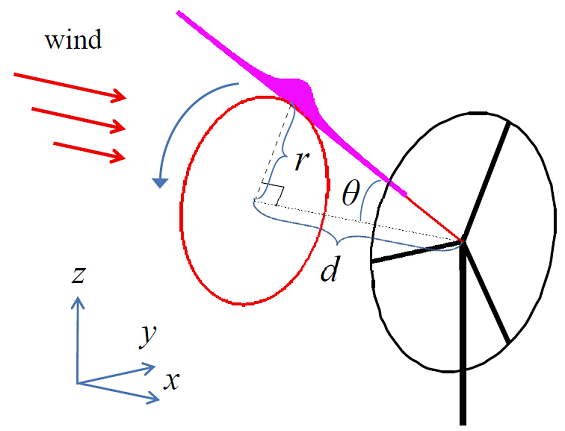
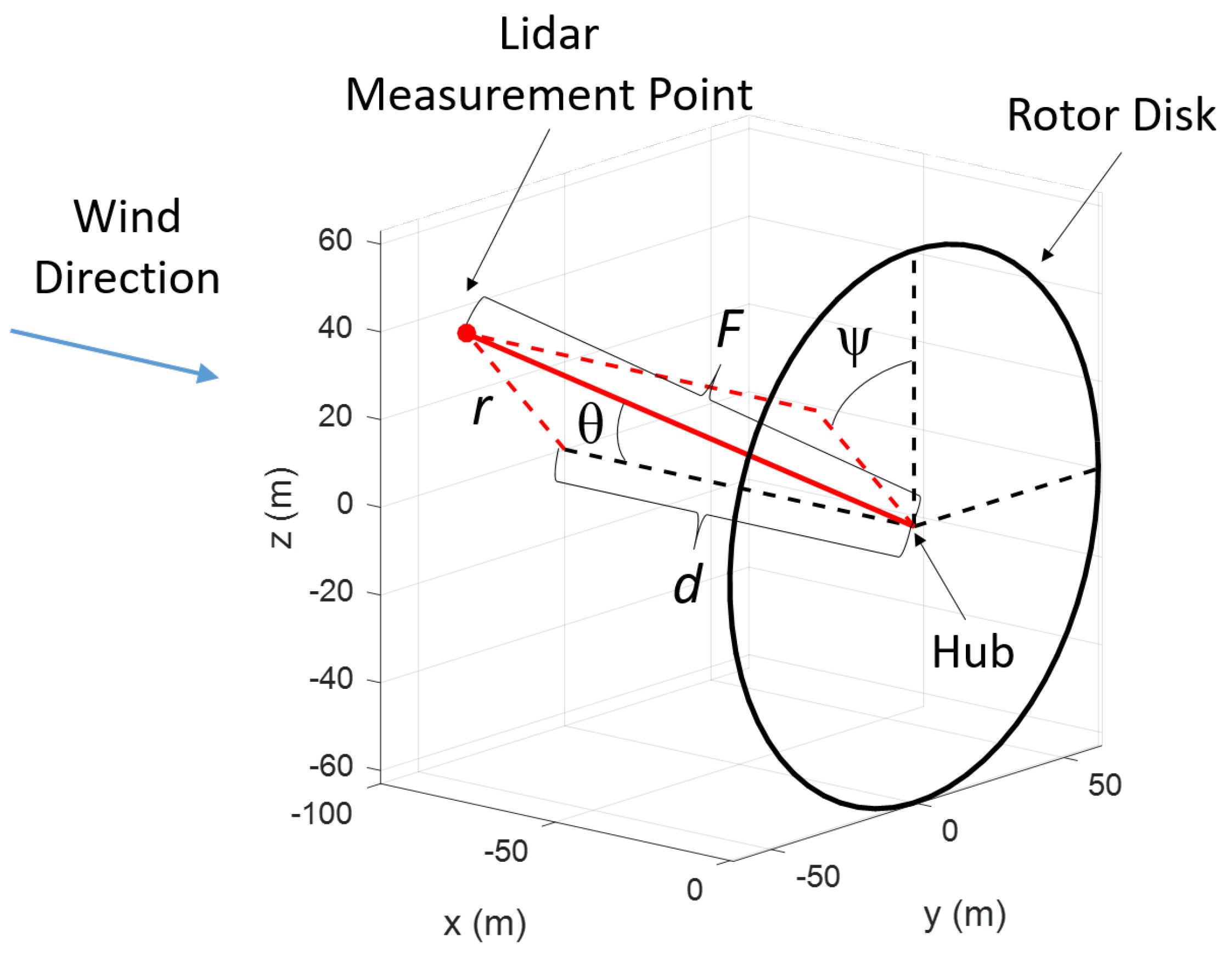
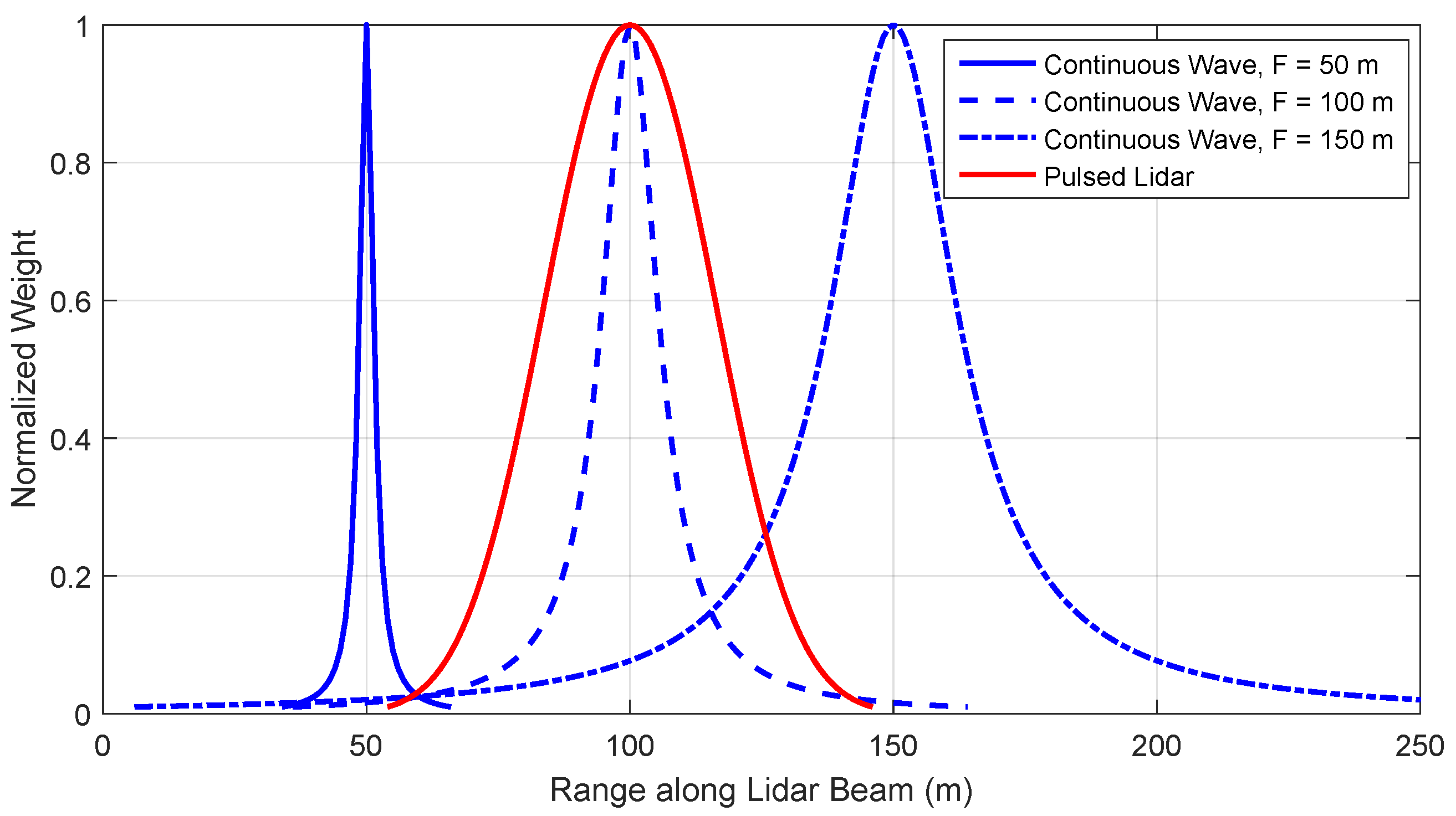
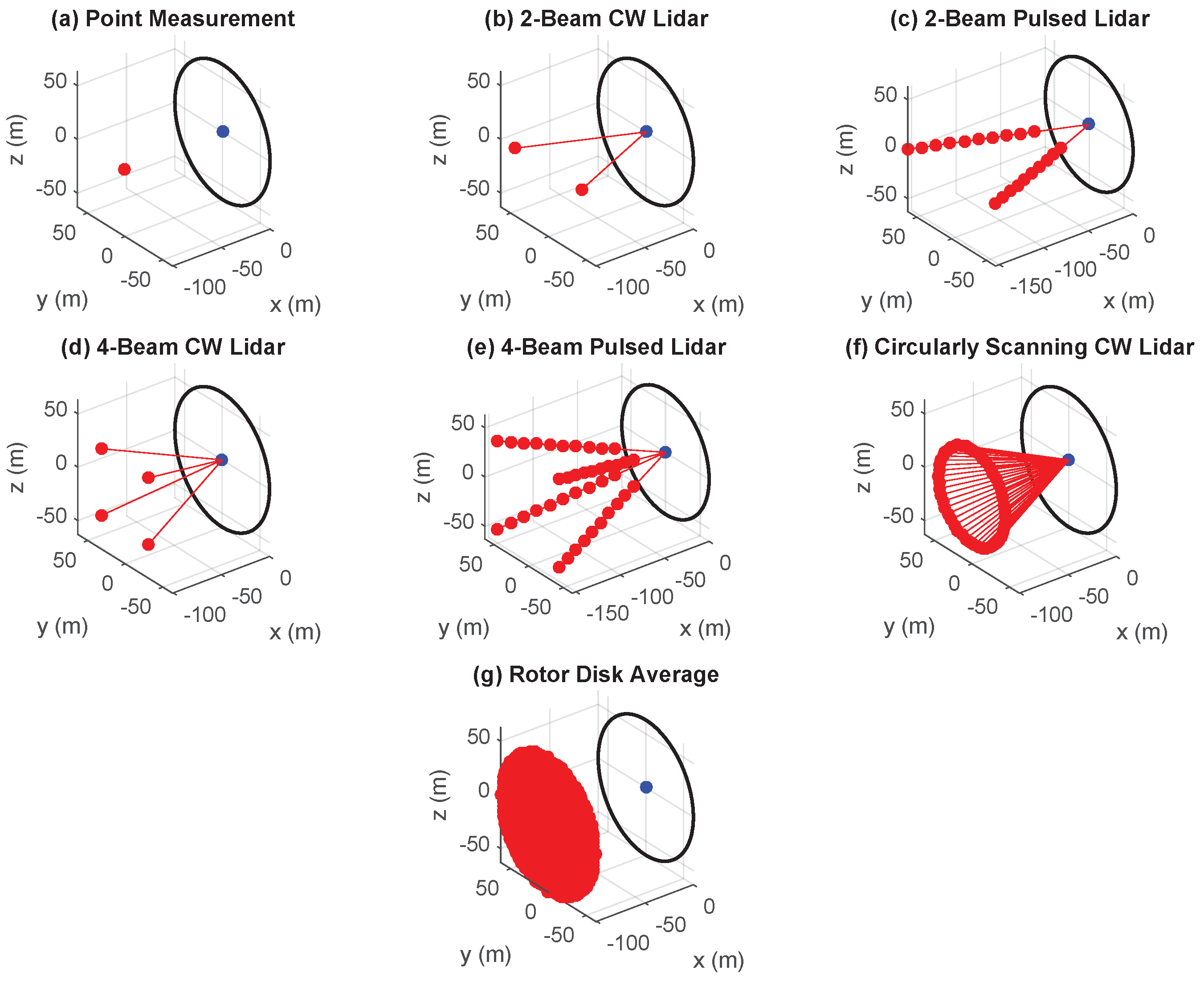
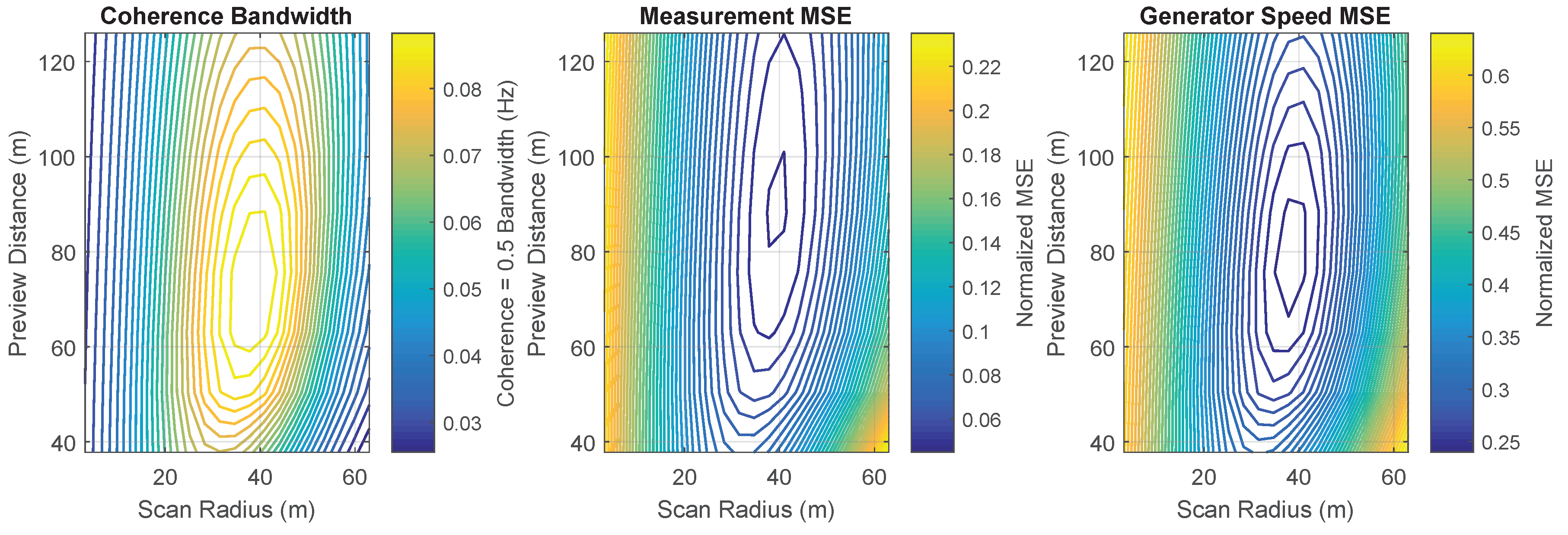
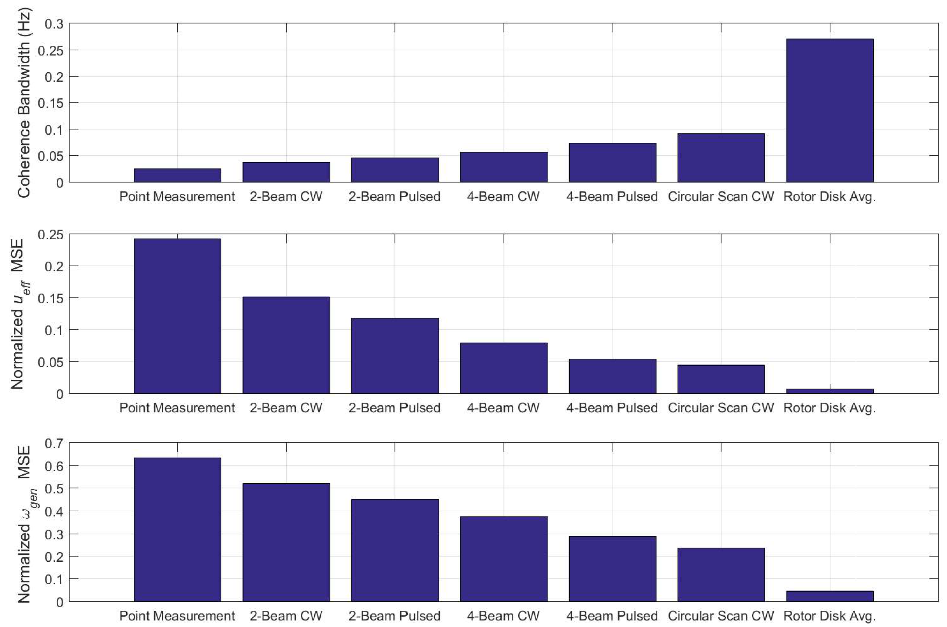
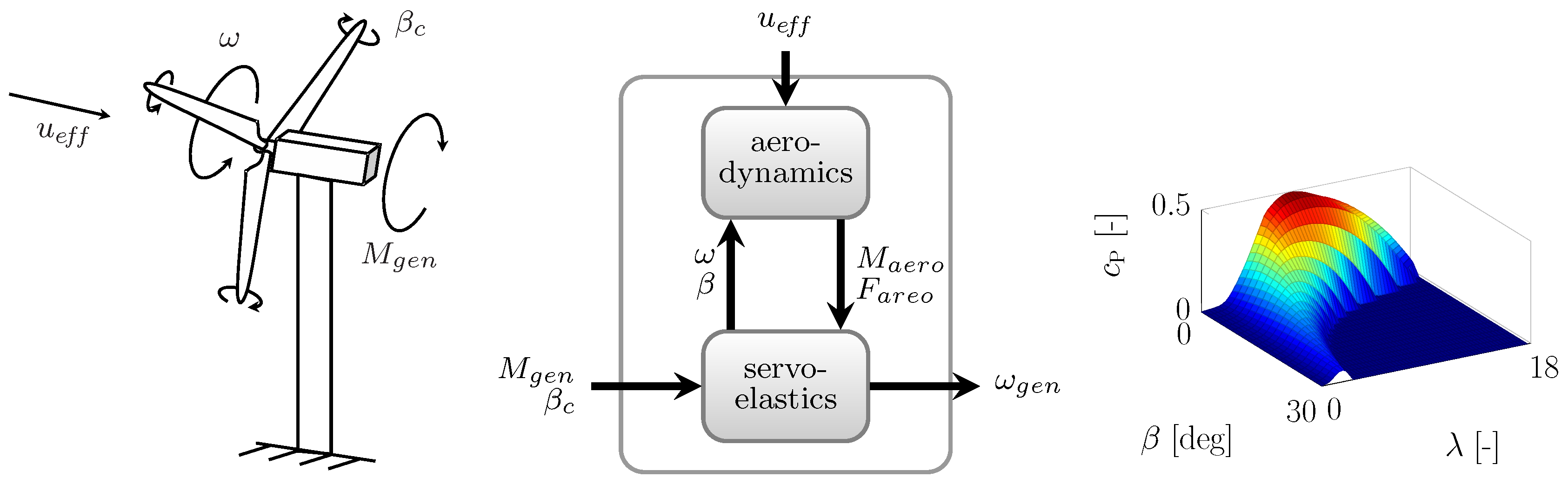
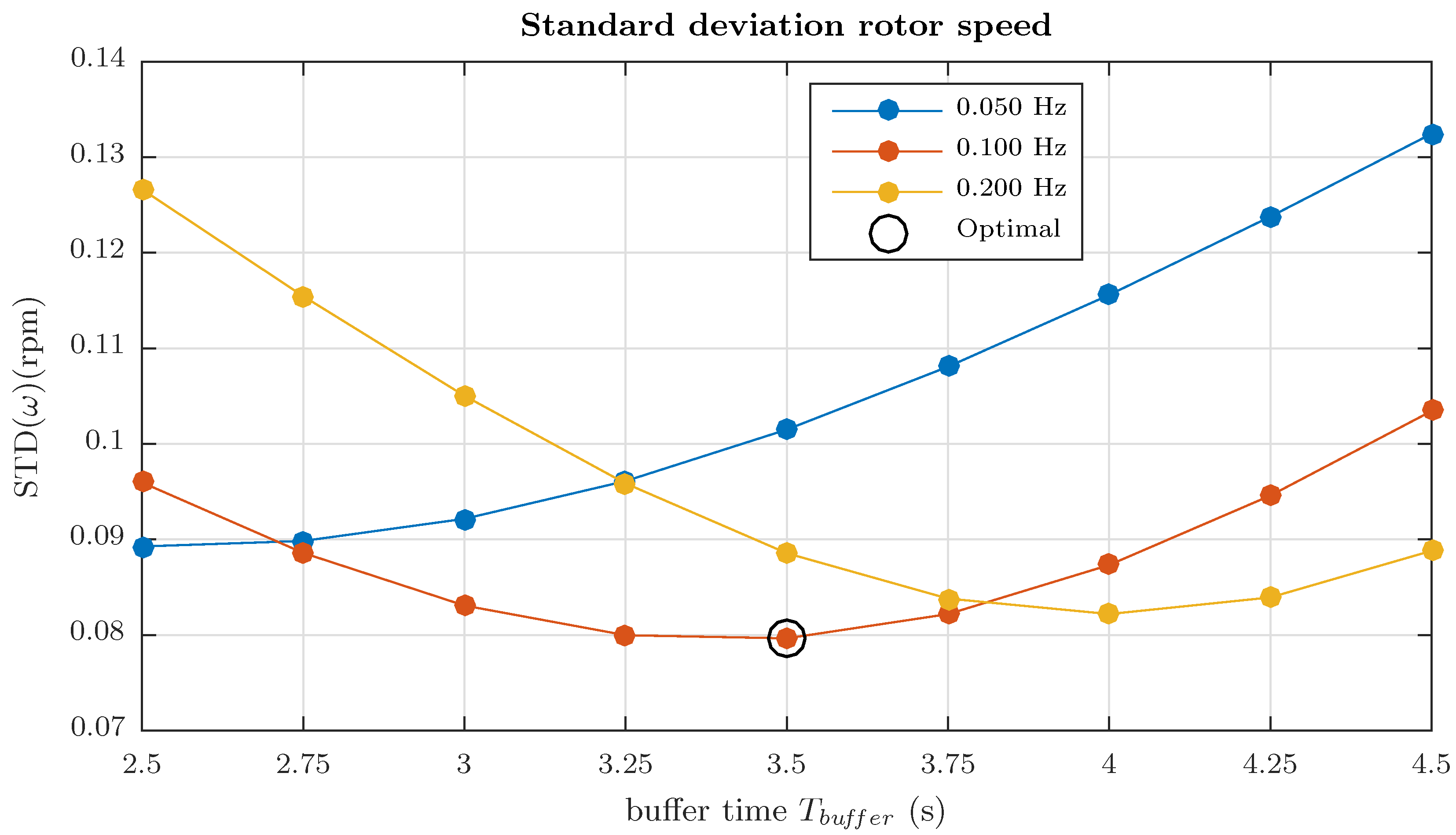
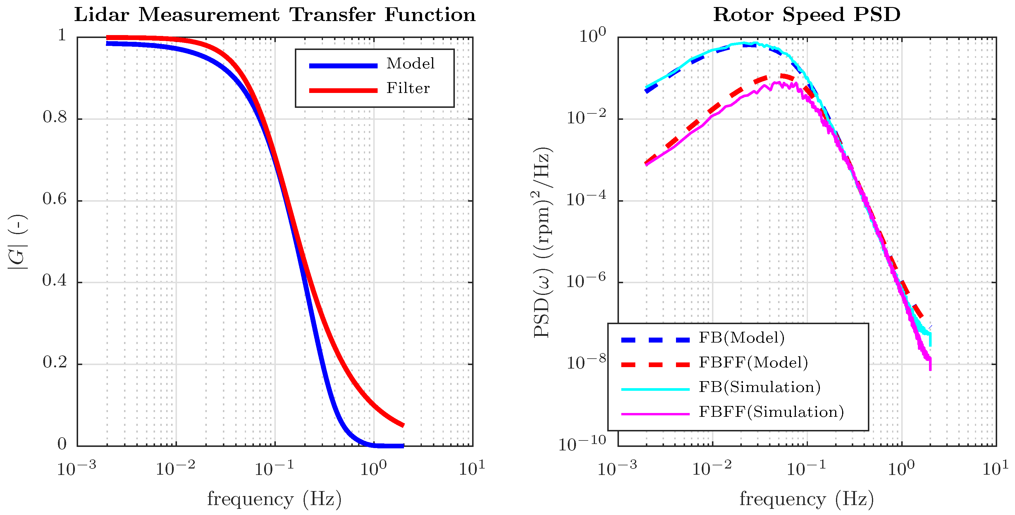