Hierarchical Fusion of Convolutional Neural Networks and Attributed Scattering Centers with Application to Robust SAR ATR

Abstract

This paper proposes a synthetic aperture radar (SAR) automatic target recognition (ATR) method via hierarchical fusion of two classification schemes, i.e., convolutional neural networks (CNN) and attributed scattering center (ASC) matching. CNN can work with notably high effectiveness under the standard operating condition (SOC). However, it can hardly cope with various extended operating conditions (EOCs), which are not covered by the training samples. In contrast, the ASC matching can handle many EOCs related to the local variations of the target by building a one-to-one correspondence between two ASC sets. Therefore, it is promising that both effectiveness and efficiency of the ATR method can be improved by combining the merits of the two classification schemes. The test sample is first classified by CNN. A reliability level calculated based on the outputs from CNN. Once there is a notably reliable decision, the whole recognition process terminates. Otherwise, the test sample will be further identified by ASC matching. To evaluate the performance of the proposed method, extensive experiments are conducted on the Moving and Stationary Target Acquisition and Recognition (MSTAR) dataset under SOC and various EOCs. The results demonstrate the superior effectiveness and robustness of the proposed method compared with several state-of-the-art SAR ATR methods.

1. Introduction

As a microwave sensor, synthetic aperture radar (SAR) has the capability to work under all-day and all-weather conditions thus providing a powerful tool for the battlefield surveillance in modern wars. A SAR system sends electromagnetic pulses from an airborne or spaceborne platform to the interested area and records the returned signals [1,2]. The range resolution of SAR images is determined by the bandwidth. In order to achieve high cross-range resolution, SAR collects data from multiple observation points, and focuses the received information coherently. Afterwards, the acquired signals are transformed into the image domain using some imaging algorithms, e.g., fast Fourier Transform (FFT) [3]. However, the main drawback of SAR images is the presence of speckles, which visually degrades the appearance of images [4]. As a result, it is difficult to interpret SAR images with high performance. As one of the key steps in SAR image interpretation, automatic target recognition (ATR) has been researched intensively since 1990s [5]. An ensemble SAR ATR system generally involves three stages: target detection [6], target discrimination [7], and target recognition [5]. A large-scale SAR image is first processed by target detection to find the potential regions of interest (ROIs), which possibly contain the interested targets. In this stage, the background clutters can be eliminated. Afterwards, target discrimination is performed to reject the false alarms in the ROIs, which are possibly caused by man-made obstacles. Finally, the selected ROIs are sent the target recognition module to determine the target labels. In this study, we focus on the third stage of the SAR ATR system, i.e., target recognition algorithms.

A typical SAR ATR algorithm generally involves two parts: feature extraction and classifier. Feature extraction aims to find low-dimensional representations for the original SAR images while maintaining the discrimination information for distinguishing different targets. In the past decades, many handcrafted features have been used for SAR ATR including the geometrical features, projection features and scattering center features. The geometrical features depict the shape and physical sizes of the target such as binary target region [8,9], target outline [10,11], shadow [12,13], etc. In [8], a region matching scheme is proposed for SAR ATR. The binary target region of the test image is directly compared with the corresponding regions from the template set. And a similarity measure is designed based on the region residuals filtered by the morphological operations. Park et al. construct 12 features based on the target outline, which are used for target recognition. The target shadow is also validated to be discriminative for SAR ATR in [10]. The projection features are obtained by projecting the original image to some specially designed basis. Typical methods for extracting the projections features are principal component analysis (PCA) [14], linear discriminant analysis (LDA) [14] and other manifold learning methods [15,16,17]. Mishra applies PCA and LDA to feature extraction of SAR images and compares their performances on target recognition [14]. The neighborhood geometric center scaling embedding is proposed in [16] by exploiting the inner structure of the training samples, which is demonstrated to be effective for SAR ATR. The scattering center features reflect the electromagnetic scattering characteristics of the target such as attributed scattering centers (ASCs) [18,19]. ASCs describe the local structures of the target by several physically relevant parameters, which have been demonstrated notably effectively for SAR ATR especially under the extended operating conditions (EOCs) [19,20,21,22,23,24,25]. In [21], an ASC-matching method is proposed based on Bayesian theory with application to target recognition. Ding et al. propose several ways to apply ASCs to SAR ATR, e.g., one-to-one ASC matching [22,23,24] and ASC-based target reconstruction [25]. Recently, the 3-D scattering center model-based SAR ATR methods have drawn the researchers’ interests, where a 3-D scattering center model is established to describe the target’s electromagnetic scatterings for feature prediction [26,27]. In the classification stage, the extracted features are classified by the classifiers to determine the target type of the test sample. With the fast development of pattern recognition and machine learning techniques, many advanced classifiers have been successfully applied to SAR ATR including adaptive boosting (AdaBoost) [28], discriminative graphical model [29], support vector machines (SVM) [30,31] and sparse representation-based classification (SRC) [32,33]. Specially, for the features without unified forms, e.g., the unordered scattering centers, a similarity or distance measure is often first defined for these features. Afterwards, the target type is determined based on the maximum similarity or minimum distance [19,20,21,22,23,24].

Recently, deep learning has been shown to provide a powerful classification scheme for image interpretation, i.e., convolutional neural networks (CNN). CNN considers the feature extraction and classification in a unified framework. As validated in several studies [34,35,36], the learned deep features by convolution operations tend to have better discrimination capability to distinguish different classes of targets. However, it should be noted that the performance of CNN is closely related to the completeness and coverage of the training samples. In the case of SAR ATR, the training samples are quite scarce due to the limited accesses to the resources [37,38]. Moreover, the operating conditions in SAR ATR are also complicated. There are many EOCs in the real-world environment including the variations of the target itself, background environments, SAR sensors, etc., which can hardly be covered by the training samples [5]. As reported in several CNN-based SAR ATR methods [39,40,41,42], they could achieve notably high recognition accuracies under the stand operating condition (SOC). However, the performances degrade ungracefully under various EOCs even with different types of data augmentations. With little prior information about the operating conditions of the test samples, it is hard to evaluate whether the decisions from CNN are reliable or not.

In this study, a SAR ATR method is proposed via hierarchical fusion of CNN and ASC matching. For each test sample, it is first classified by CNN. Based on the outputs of CNN, e.g., the pseudo posterior probabilities from softmax, a reliability level is calculated to evaluate the reliability of the decision. A preset threshold is used to judge whether the decision should be adopted. When the decision is justified to be invalidated, the test sample is passed to the classifier based on ASC matching. ASCs are local descriptors with rich, physically relevant information. It is demonstrated that ASCs can be handle various EOCs with good performances [20,21,22,23,24]. For the test samples, which cannot be reliably classified by CNN, they are possibly from EOCs. Therefore, ASC matching tends to achieve more reliable decisions for these samples. In this study, a one-to-one correspondence between the ASC set from the test image and those from the corresponding template is built using the Hungarian algorithm [22,43]. Afterwards, a similarity measure is defined, which comprehensively considers the possible outliers. Finally, the target type of the test sample is decided to be the class with the maximum similarity. Therefore, the hierarchical fusion of CNN and ASC matching can enhance both the effectiveness and robustness of the ATR method. In addition, via the hierarchical fusion, the strict demand on a single classifier is relieved. Although CNN and ASC matching may not achieve very good performances individually, they can complement each other to achieve a much better result. The main advantages of the proposed method are as follows. First, the excellent performance of CNN for SOC recognition can be inherited in the proposed method. When a reliable decision is obtained by CNN, no further classification by ASC matching is necessary. Second, the robustness of ASCs to various EOCs can be maintained in the proposed method. By building a one-to-one correspondence between two ASC sets, the local variations of the target caused by EOCs can be sensed.

The remainder of this paper is organized as follows. Section 2 describes the basic theory of CNN and the architecture of our networks. In Section 3, the classification scheme based on ASC matching is introduced. The detailed implementation of the proposed target recognition method is explained in Section 4. Extensive experiments on the Moving and Stationary Target Acquisition and Recognition (MSTAR) dataset are conducted in Section 5. Discussions are made in Section 6 to explain the reasonability of the proposed method and some future directions are stated. Conclusions are summarized in Section 7 based on the experimental results.

2. CNN

2.1. Basic Theory

Owing to the fast development of deep learning techniques, CNN has become the most prevalent tool for image interpretation [34,35,36]. CNN combines the feature learning and classification in a unified framework thus avoiding the design of hand-crafted features. In detail, the convolution layers learn hierarchical features via the convolutional operations. In the classification stage, a multilayer perceptron classifier is used for decision making.

In the convolutional layer, the previous layer’s input feature maps $O_m^{(l-1)}(m=1,\cdots ,M)$ are connected to all the output feature maps $O_n^{(l)}(n=1,\cdots ,N)$. Denote $O_m^{(l-1)}(x,y)$ and $O_n^{(l)}(x,y)$ as the unit of the $m\mathrm{th}$ input feature map and the $n\mathrm{th}$ output feature map at the position $(x,y)$, respectively, then each unit in the output feature map is calculated as:

$$O_n^{(l)}(x,y)=\sigma ({\displaystyle \sum _{m=1}^M{\displaystyle \sum _{p,q=0}^{F-1}{k}_{nm}^{(l)}(p,q)}}{O}_m^{(l-1)}(x-p,y-q)+b_n^{(l)})$$

(1)

where $k_{nm}^{(l)}(p,q)$ denotes the convolutional kernel; $\sigma (·)$ represents the nonlinear activation function and $b_n^{(l)}$ is the bias.

After the convolution layer, the pooling operation is usually performed, which cannot only effectively reduce the computational load but also make networks robust to some nuisance conditions like translation, distortion, etc. Different types of pooling operations are used in CNNs by either choosing the average or maximum in a preset window with the sizes of $h\times w$. For example, the max pooling is defined as follow.

$$O_m^{(l+1)}(x,y)=\underset{1<i<h,1<j<r}{\max }(O_m^{(l)}(x+i,y+j))$$

(2)

In the classification stage, the softmax nonlinearity is applied to the output layer to determine the target label. It will output the posterior probabilities over each class and the target label will be decided as the class with the maximum probability.

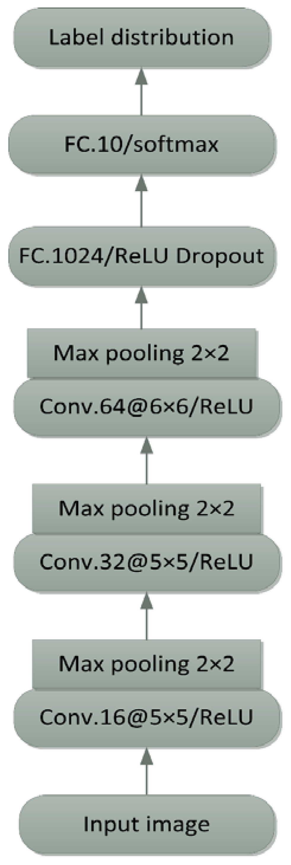
2.2. Architecture of the Proposed CNN

Actually, there is no consensus on how to design CNNs for the specific application of SAR ATR. In the previous works, several different kinds of CNNs have been applied to SAR ATR and they all achieved very good performances [39,40,41,42]. Based on these works, this paper designs the architecture of CNN as Figure 1, which is composed of three convolution layers, three max pooling layers, and two fully-connected layers. The convolution stride is fixed to 1 pixel with no spatial zero padding. After each convolution layer, a max pooling is performed with a kernel size of 2 × 2 and a stride of 2 pixels. The rectified linear units (ReLU) activation function is applied to every hidden convolution layer.

Specifically for the MSTAR dataset used in this study, all the images are first cropped to be 88 × 88 patches from the centroid. The detailed layout of our network is displayed in

Table 1. Layout of the proposed CNN.

Layer Type	Image Size	Feature Maps	Kernel Size
Input	88 × 88	1	-
Convolution	84 × 84	16	5 × 5
Pooling	42 × 42	16	2 × 2
Convolution	38 × 38	32	5 × 5
Pooling	19 × 19	32	2 × 2
Convolution	14 × 14	64	6 × 6
Pooling	7 × 7	64	2 × 2
Full Connected	1 × 1	1024	-
Output	1 × 1	10	-

. The input image is filtered by 16 convolution filters with the size of 5 × 5 in the first convolution layer, producing 16 feature maps with the size of 84 × 84. After the first pooling layer, their sizes become 42 × 42. After the second convolution layer, there are 32 feature maps with size of 38 × 38, which become 19 × 19 after pooling. After the third convolution layer and pooling layer, 64 feature maps with the size of 7 × 7 are obtained. In the first fully-connected layer, a 1024-dimensionality vector is produced, where the dropout regularization technique is used. The output layer is also a fully-connected layer with the softmax function to ensure the final output size to be 1 × 1 × 10, corresponding to the probabilities of the 10 classes of MSTAR targets.

During the training of the designed networks, the weights are initialized from Gaussian distributions with zero mean and a standard deviation of 0.01, and biases are initialized with a small constant value of 0.1. The learning rate is initially 0.001, which decreases by a factor of 0.1 after 100 epochs. The batch size is set to be 100. To train the proposed CNN, the deep learning toolbox in Tensorflow is used. The cropped MSTAR training images (the detailed descriptions of the MSTAR dataset are presented in Section 5) are fed to the networks in Figure 1. The hierarchical features are learned during the training process. According to the target label of each training sample, the parameters of the whole networks are obtained. As shown in Figure 2, the total loss decreases sharply and converges after about 1500 epochs during the training. Figure 3 illustrates the original image and internal state of the trained CNN. In the first convolution layer, the convolution kernels and 16 feature maps are shown in Figure 3b,c, respectively. It is clearly that the global properties of the original image in Figure 3a can be maintained in the feature maps. Afterwards, in the classification stage, the cropped test image is input to the trained CNN to decide its target type.

3. ASC Matching

3.1. ASC Model

The high-frequency scattering of an electrically large target can be well approximated as a sum of the responses from individual scattering centers as Equation (3) [18].

$$E(f,\varphi ;\theta )={\displaystyle \sum _{i=1}^K{E}_i(f,\varphi ;{\theta }_i)}$$

(3)

where $f$ denotes the frequency and $\varphi$ represents the aspect angle. The backscattering field of a single scattering center can be described by the ASC model as follows.

$$\begin{array}{ll}{E}_i(f,\varphi ;{\theta }_i)=& A_i\cdot {(j\frac{f}{f_c})}^{{\alpha }_i}\cdot \exp (\frac{-j4\pi f}{c}(x_i\cos \varphi +y_i\sin \varphi ))\\ & \cdot \sin \mathrm{c}\left(\frac{2\pi f}{c}{L}_i\sin \right(\varphi -\overline{{\varphi }_i}\left)\right)\cdot \exp (-2\pi f{\gamma }_i\sin \varphi )\end{array}$$

(4)

In Equation (4), $\theta =\left\{{\theta }_i\right\}=[A_i,{\alpha }_i,x_i,y_i,L_i,\overline{{\varphi }_i},{\gamma }_i](i=1,2,\cdots ,K)$ is the parameter set of the ASCs. In detail, $A_i$ denotes the complex amplitude; $\left(x_i,y_i\right)$ are the spatial positions; ${\alpha }_i$ represents the frequency dependence; $L_i$ and $\overline{{\varphi }_i}$ are the length and orientation of the distributed ASC, respectively and ${\gamma }_i$ is the aspect dependence of the localized ASC. The ASC attributes provide rich physically relevant descriptions for the local structures of the target. $\left(x_i,y_i\right)$ denotes the scattering center location in the image domain. ${\alpha }_i$ is a discrete parameter, which takes on integer or half-integer values. Some typical values of ${\alpha }_i$ are 1, 1/2, 0, −1, −2. The combination of the length and frequency dependency can effectively reveal the geometrical structure of the ASC. For example, when ${\alpha }_i$ is 1 and $L_i$ is nonzero, the ASC is assumed to have a dihedral shape. More explanations can be referred to [18].

3.2. Sparse Representation for ASC Extraction

For a single SAR image, there are only a few ASCs in the target. When the parameter space is gridded to form an over-complete dictionary, the parameter estimation of ASCs can be formulated as a sparse representation problem [44,45]. Firstly, Equation (3) is rewritten as

$$s=D(\theta )\times \sigma$$

(5)

In Equation (5), $s$ is the vector form of the measurements $E(f,\varphi ;\theta )$; $D(\theta )$ is modeled as a parameterized redundant dictionary, in which each column is the vectorization of the measurements corresponding to one element in parameter set $\theta$; $\sigma$ is a complex sparse vector whose element represents the relative amplitude $A$. Considering the possible noises during the data acquisition, the real measurements should be expressed as

$$s=D(\theta )\times \sigma +n$$

(6)

where $n$ is modeled as the additive white Gaussian noise with zero mean. Then, the ASCs can be extracted by solving the following problem:

$$\widehat{\sigma }=\underset{\sigma }{\arg \min }{\Vert \sigma \Vert }_0,\mathrm{s}.\mathrm{t}. {\Vert s-D(\theta )\times \sigma \Vert }_2\le \epsilon$$

(7)

where $\epsilon ={\Vert n\Vert }_2$ represents the noise level, which can be estimated from the original measurements; ${\Vert •\Vert }_0$ denotes $l_0$-norm and $\widehat{\sigma }$ is the complex-valued amplitude estimator with respect to dictionary $D(\theta )$. The optimization problem in Equation (7) is nondeterministic polynomial time hard (NP-hard), which is computationally difficult to solve. However, an approximation solution can be obtained by some greedy algorithms, such as the orthogonal matching pursuit (OMP) [45]. The detailed implementation of ASC extraction using OMP is described in Algorithm 1, which is used in this study.

Algorithm 1 OMP for ASC Extraction

Input: The measurements $s$, estimated noise level $\epsilon$, and redundant parameterized dictionary $D(\theta )$. Initialization: The initial parameter set of the ASCs $\widehat{\theta }=\varnothing$, reconstruction residual $r=s$, and iteration counter $t=1$. 1. while ${\Vert r\Vert }_2^2>\epsilon$ do 2. Calculate correlation: $C(\theta )=D^H(\theta )\times r$, where ${(·)}^H$ denotes conjugate transpose. 3. Estimate parameters: ${\widehat{\theta }}_t=\underset{\theta }{\arg \min }C(\theta )$, $\widehat{\theta }=\widehat{\theta }{\displaystyle \cup {\widehat{\theta }}_t}$. 4. Estimate amplitudes: $\widehat{\sigma }=D^{†}(\theta )\times s$, where ${(·)}^{†}$ denotes the Moore-Penrose pseudo-inverse, $D(\widehat{\theta })$ represents the dictionary constructed by the parameter set $\widehat{\theta }$. 5. Update residual: $r=s-D(\widehat{\theta })\times \widehat{\sigma }$. 6. $t=t+1$ Output: The estimated parameters set $\widehat{\theta }$.

3.3. ASC Matching

The ASCs contain rich physically relevant descriptions for the local structures of the target such as the relative amplitude, spatial positions, length, etc. Therefore, the ASCs can be effectively used to sense the local variations of the target caused by various EOCs like configuration variance, depression angle variance, partial occlusion, etc. In this study, an ASC matching method is proposed for target recognition. A one-to-one correspondence between two ASC sets is first established. Then, the matched ASC pairs are evaluated to form a similarity measure for target recognition.

3.3.1. One-To-One Matching between ASC Sets

(1)

Distance measure for two individual ASCs

An essential prerequisite to build the one-to-one correspondence is properly evaluation the distance between two individual ASCs. This paper uses four attributes, i.e., $[A,x,y,L]$, for distance evaluation because of their clearly physical meanings and stability during the ASC extraction. For the test ASC set $P=[p_1,p_2,\dots ,p_M]$ and template ASC set $Q=[q_1,q_2,\dots ,q_N]$, the distance between two individual ASCs is defined as follow:

$$d(p_i,q_j)=\left[{(p_{ix}-q_{jx})}^2+{(p_{iy}-q_{jy})}^2+\frac{{(p_{iL}-q_{jL})}^2}{2}\right]\ast \exp \left(\frac{|p_{iA}-q_{jA}|}{2}\right)$$

(8)

According to Equation (8), the distance is explained as three components. The first is the Euclidean distance between the spatial positions, i.e., $[{(p_{ix}-q_{jx})}^2+{(p_{iy}-q_{jy})}^2]$. The second is the difference between the lengths, i.e., $\frac{{(p_{iL}-q_{jL})}^2}{2}$. The attribute $L$ is assumed to have twofold uncertainty than the spatial positions because it is more difficult to obtain a better estimation of the parameter. For the amplitude $A$, it is first normalized based on its absolute and the distance is measured by an exponential function.

(2)

ASC matching using the Hungarian algorithm

Based on the designed distance measure, this study uses the Hungarian algorithm to build the one-to-one correspondence between two ASC sets. As a bipartite graph matching problem, the Hungarian algorithm can find the best one-to-one correspondence between two point sets with the lowest total distance [43].

The cost matrix for Hungarian matching is displayed in

Table 2. Cost matrix for Hungarian matching.

	$q_1$  $q_2$  $\cdots$   $q_N$	FA
$p_1$	$C_{11}$  $C_{12}$  $\cdots$  $C_{1N}$	$f_1$    $\infty$ $\cdots$   $\infty$
$p_2$	$C_{21}$  $C_{22}$  $\cdots$   $C_{2N}$	$\infty$    $f_2$ $\cdots$   $\infty$
$⋮$	$⋮$   $⋮$  $\ddots$    $⋮$	$⋮$    $⋮$  $\ddots$  $⋮$
$p_M$	$C_{M1}$  $C_{M2}$ $\cdots$  $C_{MN}$	$\infty$    $\infty$  $\cdots$  $f_M$
MA	$m_1$   $\infty$  $\cdots$  $\infty$	$\infty$     $\infty$  $\cdots$ $\infty$
	$\infty$   $m_2$  $\cdots$  $\infty$	$\infty$     $\infty$  $\cdots$ $\infty$
	$⋮$   $⋮$   $\ddots$   $⋮$	$⋮$      $⋮$  $\ddots$  $⋮$
	$\infty$   $\infty$  $\cdots$  $m_N$	$\infty$     $\infty$  $\cdots$ $\infty$

, where $C_{ij}=d(p_i,q_j)$. In this study, the absolute amplitudes of different ASCs are subject to amplitude normalization in both ASC sets. The cost of assigning $p_i$ to $q_j$ is the defined distance in Equation (8). In practical applications, the test ASC set may contain some false ASCs caused by the background noises. In addition, the template ASC set may have some missing ASCs due to the deformation of the test target such as partial occlusion. Therefore, the false ASCs (false alarms, FAs) and missing ASCs (missing alarms, MAs) should be considered during the Hungarian matching. The costs for the FAs and MAs contained in Table 2 are defined as follows.

$$f_i=\frac{1}{M}{\displaystyle \sum _{j=1}^M{C}_{ji}}, m_i=\frac{1}{N}{\displaystyle \sum _{j=1}^N{C}_{ij}}$$

(9)

The cost of assigning an test ASC to be a FA is the average of assigning it to all $q_i(i=1,2,\cdots ,N)$ and a template ASC to a MA is the average of assigning it to all $p_j(j=1,2,\cdots ,M)$. To form a complete bipartite graph for Hungarian matching, some costs in Table 2 are assigned as “$\infty$” (i.e., infinity). The “$\infty$” costs can effectively constraint unsuitable matched pairs. For example, the MAs will not be matched with the FAs.

3.3.2. Similarity Evaluation

Based on the one-to-one correspondence built by Hungarian matching, both the matched ASC pairs and possible outliers are considered to define the similarity measure for two ASC sets as Equation (10).

$$S(P,Q)=\frac{2K_m}{M+N}\ast \exp \left(-{\displaystyle \sum _{k=1}^{K_m}\left({\omega }_k\ast d_k\right)}\right)$$

(10)

where $K_m$ denotes the number of matched ASC pairs; $d_k$ represents the distance between the $k\mathrm{th}$ matched pairs, which can be referred from the cost matrix, and ${\omega }_k$ is the corresponding weight defined as follow.

$${\omega }_k=\frac{A_k}{{\displaystyle \sum _{k=1}^{K_m}{A}_k}}$$

(11)

In Equation (11), $A_k$ denotes the absolute amplitude of the matched test ASC. The test ASCs are taken as the baseline because they are compared with different types of template ASC sets. The weights are defined based on the relative amplitudes for the following considerations. On one hand, the strong ASCs with higher amplitudes tend to be more stable during the ASC extraction. On the other hand, the ASCs with higher amplitudes will keep more stable under noise corruption or other interferences. With the deterioration of noise corruption, the ASCs with lower amplitudes are more probable to be submerged. Therefore, by assigning higher weights to the stronger ASCs, the similarity measure will be more robust to the possible uncertainties during ASC extraction and noise corruption.

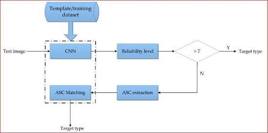
4. Hierarchical Fusion of CNN and ASC Matching for SAR ATR

As reported in relevant literatures [39,40,41,42], CNN can achieve notably high accuracies under SOC or the conditions similar to SOC. The ASC matching is more robust to those conditions with local variations caused by EOCs like noise corruption, configuration variance, partial occlusion, etc. To combine their merits in a unified ATR system, a hierarchical fusion framework is proposed in this study.

Figure 4 shows the general procedure of the proposed target recognition method. First, the test sample is classified by the designed CNN. The pseudo posterior probabilities from the softmax are used to define a reliability level as follow:

$$\{\begin{array}{l}{P}_k=\max ([P_1 P_2 \cdots P_C])\\ r=\min \left(\frac{P_k}{P_i}\right)(i\ne k)\end{array}$$

(12)

where $P_i(i=1,2,\cdots ,C)$ denotes the probability corresponding to the $i\mathrm{th}$ class; $r$ represents the reliability of the decision with a value larger than 1, which reflects the difference between the highest probability with the second highest one. A larger $r$ indicates a more reliable decision.

A threshold $T$ is used to judge whether the decision from CNN should be adopted. With a reliability level higher than the threshold, the decision is assumed to be highly reliable. Then, the target type is directly decided by CNN. Otherwise, the test sample is passed to the ASC matching for further identification. The template samples are selected based on the estimated azimuth of the test image [19]. Then, the target type is decided to be the class with the maximum similarity. The ASC matching makes detailed analysis about the local structures of the targets thus more robust to various EOCs. By hierarchically fusing the two classification schemes, both the efficiency and robustness of the ATR method can be enhanced.

5. Experiment

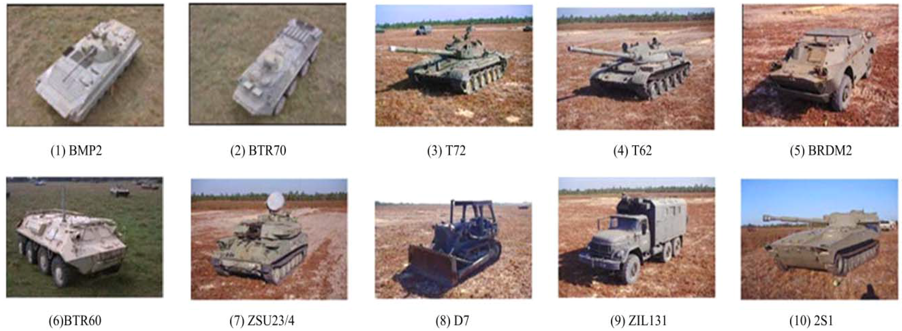
5.1. Data Preparation and Experimental Setup

To experimentally evaluate the proposed method, the MSTAR dataset is used in this study, which is the benchmark dataset for SAR ATR. There are 10 military targets included in the dataset, which share similar appearances as shown in Figure 5. Their SAR images are captured by the X-band SAR sensors with the resolution of 0.3 m × 0.3 m. The training and test samples used for experiments are showcased in

Table 3. Training and test sets used in the experiments.

Class	Serial No.	Training Set		Test Set
		Depression	No. Images	Depression	No. Images
BMP2	9563	17°	233	15°	195
	9566	17°	232	15°	196
	c21	17°	233	15°	196
BTR70	c71	17°	233	15°	196
T72	132	17°	232	15°	196
	812	17°	231	15°	195
	S7	17°	228	15°	191
ZSU23/4	D08	17°	299	15°	274
ZIL131	E12	17°	299	15°	274
T62	A51	17°	299	15°	273
BTR60	k10yt7532	17°	256	15°	195
D7	92v13015	17°	299	15°	274
BDRM2	E71	17°	298	15°	274
2S1	B01	17°	299	15°	274

, which are collected at 17° and 15° depression angles, respectively.

For performance comparison, several state-of-the-art SAR ATR methods are used including SVM [30], SRC [32] and A-ConvNet [39], as briefly described in

Table 4. Reference methods for comparison.

Abbre.	Feature	Classifier	Ref.
SVM	PCA features	SVM	[30]
SRC	PCA features	SRC	[32]
A-ConvNet	Original image intensities	CNN	[39]
ASC	ASCs	ASC matching method	[22]

. SVM and SRC are performed on 80-dimension PCA feature vectors extracted from the original images. A-ConvNet in [29] is chosen as the representative of the CNN-based SAR ATR methods. The ASC matching method proposed in [22] is also compared, where a one-to-one correspondence between two ASC sets is built for similarity evaluation. In the followings, the experiment is first conducted under SOC on the 10 classes of targets. Afterwards, several typical EOCs are used to comprehensively evaluate the robustness of the proposed method including configuration variance, large depression angle variance, noise corruption and partial occlusion. Finally, the performance is evaluated under limited training samples to further examine it robustness.

5.2. Recognition under SOC

5.2.1. Preliminary Verification

The recognition problem is first considered under SOC. The 10-class training and test samples in Table 3 are used. The threshold $T$ for the reliability level is first set to be 1.1.

Table 5. Confusion matrix of the proposed method under SOC.

Class	BMP2	BTR70	T72	T62	BDRM2	BTR60	ZSU23/4	D7	ZIL131	2S1	PCC (%)
BMP2	194	0	0	0	0	0	1	0	0	0	99.49
BTR70	0	196	0	0	0	0	0	0	0	0	100
T72	0	1	194	0	0	0	1	0	0	0	98.98
T62	0	0	0	271	0	0	2	0	0	0	99.27
BDRM2	0	0	1	0	271	1	1	0	0	0	98.91
BTR60	0	1	0	1	0	193	0	0	0	0	98.97
ZSU23/4	0	0	0	0	0	0	274	0	0	0	100
D7	0	0	0	1	1	0	0	272	0	0	99.27
ZIL131	0	0	0	0	0	0	1	0	274	0	100
2S1	0	0	0	1	0	0	0	0	1	272	99.27
Average (%)	99.41

displays the detailed recognition results of the proposed method. Each of the 10 targets can be classified with a percentage of correct classification (PCC) over 98%.

Table 6. Comparison of different methods under SOC.

Method	Proposed	SVM	SRC	A-ConvNet	ASC
PCC (%)	99.41	98.42	97.66	99.12	97.30

compares the average PCCs of different methods under SOC. With the highest PCC of 99.41%, the proposed method outperforms the others with notable margins. A-ConvNet ranks second in all the methods, indicating the excellent classification capability of CNN. Under SOC, the training and test samples are quite similar with only a small depression angle variance (2°) in this case. Therefore, most test samples can be correctly classified by CNN because of its powerful classification capability. Due to the unpredictable factors during data acquisition, a few test samples may have many differences with the training samples. As a result, they may not be reliably determined by the designed CNN. Then, they are passed to ASC matching for further determination. By combining the advantages of the two classification schemes, the final recognition performance of the proposed method is largely enhanced.

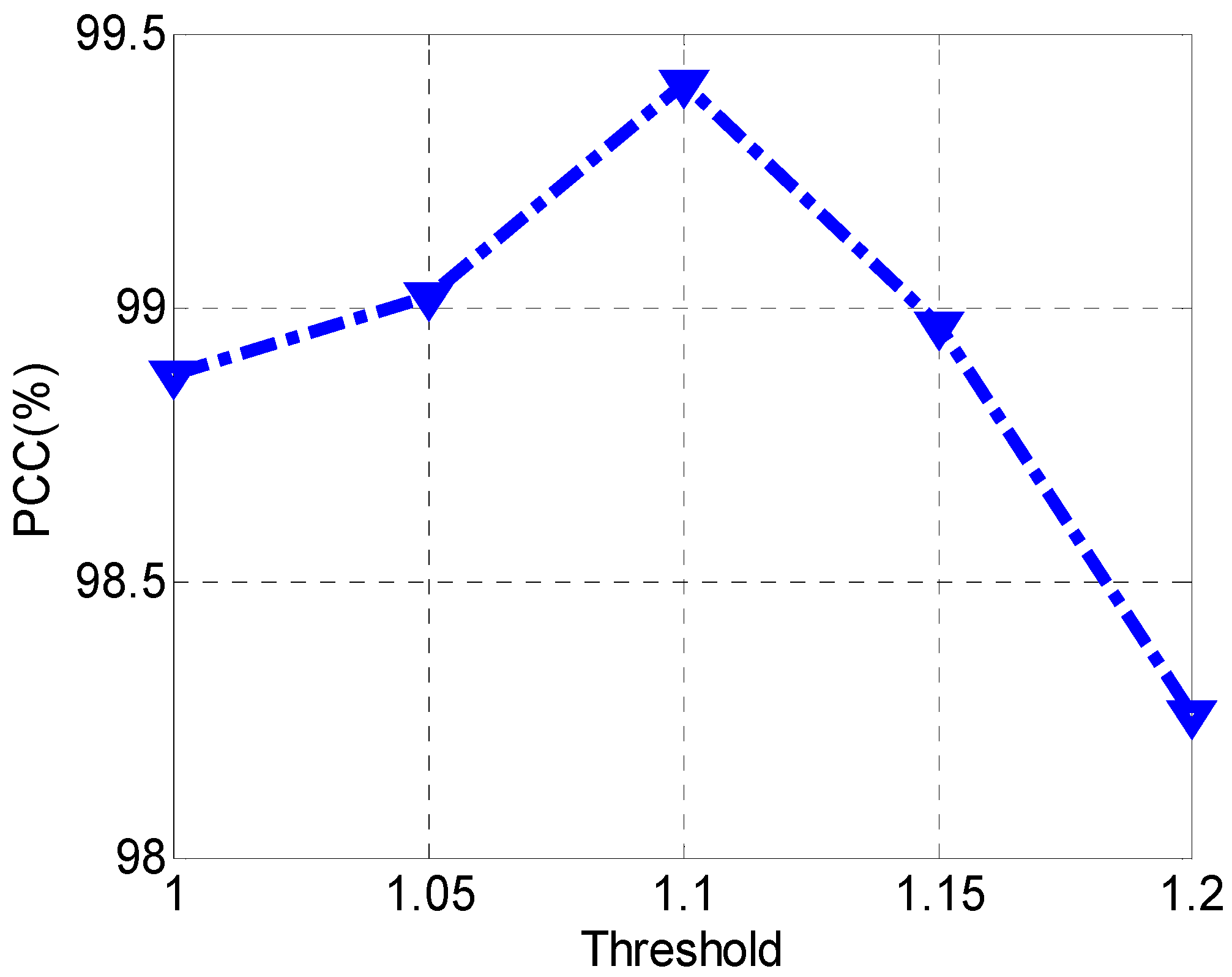
5.2.2. Performance under Different Thresholds

The threshold $T$ directly determines whether the decision from CNN is reliable. Therefore, it has important influences on the final recognition performance. By varying the threshold, the PCCs of the proposed method are plotted in Figure 6. The PCC tops at $T=1.1$ and the detailed results can be found in the former experiment. The PCC varies in the threshold interval. However, the average PCC of all the thresholds is still calculated to be 98.91%, indicating the robustness of the proposed method. When the threshold is lower than 1, all the test samples are directly classified by the designed CNN. Will a threshold slightly higher than 1, most of the test samples are determined by CNN and only a few are passed to ASC matching. Due to the excellent classification capability of CNN under SOC, the performance maintains at a high level. In contrast, when the threshold is notably high, almost all the decisions are made by ASC matching. Actually, the ASC matching is also an effective SAR ATR method. Therefore, the PCC will not fall too much. In the following experiments, the threshold is fixed to be $T=1.1$ in order to achieve better recognition performance.

5.3. Recognition under EOCs

As a reliable SAR ATR system, it must be robust to various EOCs in the real-world scenarios caused by the variations of the target itself, background environments, sensors, etc. To comprehensively evaluate the proposed method, the following experiments are conducted under different types of EOCs, i.e., configuration variance, large depression angle variance, noise corruption and partial occlusion.

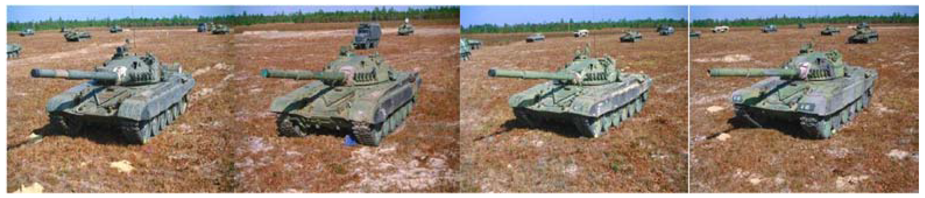
5.3.1. Configuration Variance

A certain military target may be modified to have several different configurations for different applications. The different configurations share similar target shapes with some local variations.

Table 7. Training and test sets with configuration variance.

	Depression	BMP2	BDRM2	BTR70	T72
Training set	17°	233 (Sn_9563)	298	233	232(Sn_132)
Test set	15°, 17°	428(Sn_9566) 429(Sn_c21)	0	0	426(Sn_812) 573(Sn_A04) 573(Sn_A05) 573(Sn_A07) 567(Sn_A10)

showcases the training and test sets for this experiment. The configurations of BMP2 and T72 for testing are not included in the training set. Figure 7 shows the optical images of four different configurations of T72. Several local differences can be found at the turret, fuel drums, etc.

Table 8. Recognition results of the proposed method under configuration variance.

Class	Serial No.	BMP2	BRDM2	BTR-70	T-72	PCC (%)
BMP2	Sn_9566	410	13	4	1	95.79
	Sn_c21	417	5	4	3	97.20
T72	Sn_812	13	1	1	411	96.48
	Sn_A04	15	8	0	550	95.99
	Sn_A05	12	2	2	557	97.21
	Sn_A07	8	2	10	553	97.21
	Sn_A10	12	5	0	550	97.00
Average (%)	96.61

lists the detailed recognition results of the proposed method under configuration variance. All the configurations of BMP2 and T72 can be classified with PCCs over 96%, resulting in an average of 98.64%. The performances of different methods are compared in

Table 9. Comparison of different methods under configuration variance.

Method	Proposed	SVM	SRC	A-ConvNet	ASC
PCC (%)	98.64	95.88	95.64	98.18	97.82

. With the highest PCC, the proposed method is validated to be the most robust to configuration variance. It is also notable that the ASC method outperforms the remaining ones. In the ASC method, the one-to-one correspondence between the test and template ASC sets is built, which is beneficial to sense the local variations of the target caused by configuration variance. In the proposed method, some test samples can still be reliably classified using the designed CNN. The remaining ones can obtain more accurate decisions by ASC matching. Therefore, the final recognition performance of the proposed method can be effectively enhanced.

5.3.2. Large Depression Angle Variance

The test SAR images may be collected at different depression angles with the training samples. Figure 8 shows the SAR images of 2S1 at three depression angles, i.e., 17°, 30° and 45°. It is visible that images with large depression angle variances have quite different appearances like the target shape and scattering patterns [46,47]. The training and test sets for this experiment are showcased in

Table 10. Training and test sets with large depression angle variance.

	Depression	2S1	BDRM2	ZSU23/4
Training set	17°	299	298	299
Test set	30°	288	287	288
	45°	303	303	303

, where three targets are included, i.e., 2S1, BRDM2 and ZSU23/4.

Table 11. Recognition results of the proposed method under depression variance.

Depression	Class	Results			PCC (%)	Average (%)
		2S1	BDRM2	ZSU23/4
30°	2S1	280	5	3	97.22	97.80
	BDRM2	2	283	2	98.26
	ZSU23/4	2	5	281	97.57
45°	2S1	219	53	31	72.28	76.16
	BDRM2	12	245	46	80.96
	ZSU23/4	34	41	228	75.25

presents the detailed recognition results of the proposed method at different depression angles. At 30° depression angle, the proposed method can still achieve a very high PCC of 97.80%. However, when the depression angle changes to 45°, the performance decreases significantly to 76.16%. The main reason is that the notably large depression angle variance causes much discrepancy between the training and test samples.

Table 12. Comparison of different methods under large depression angle variance.

Method	PCC (%)
	30°	45°
Proposed	97.80	76.16
SVM	96.57	61.05
SRC	96.32	65.35
A-ConvNet	96.94	63.24
ASC	96.26	71.65

compares the performances of different methods under large depression angle variance. With the highest PCCs at both depression angles, the proposed method is demonstrated to be the most robust. The ASC method ranks second in all the methods and the superiority becomes more remarkable at 45° depression angle. Although the global appearance changes greatly under large depression angle variance, some local characteristics can still maintain stable. Therefore, the ASCs can better serve for target recognition in this situation. By combing the merits of CNN and ASC matching, the proposed method achieves the best performance.

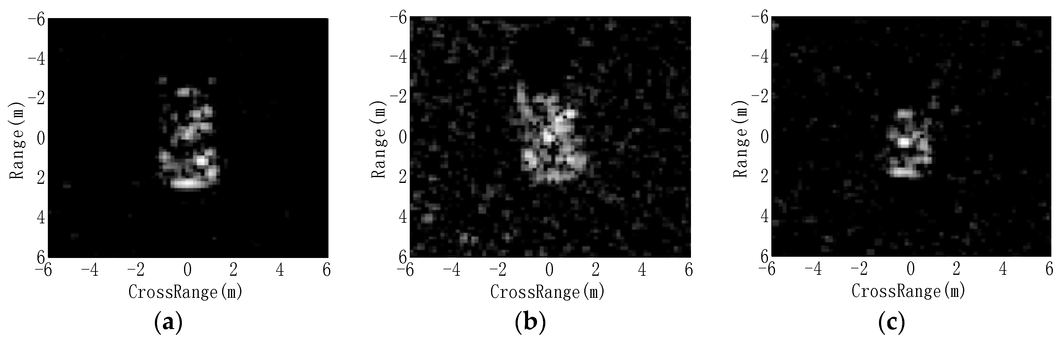
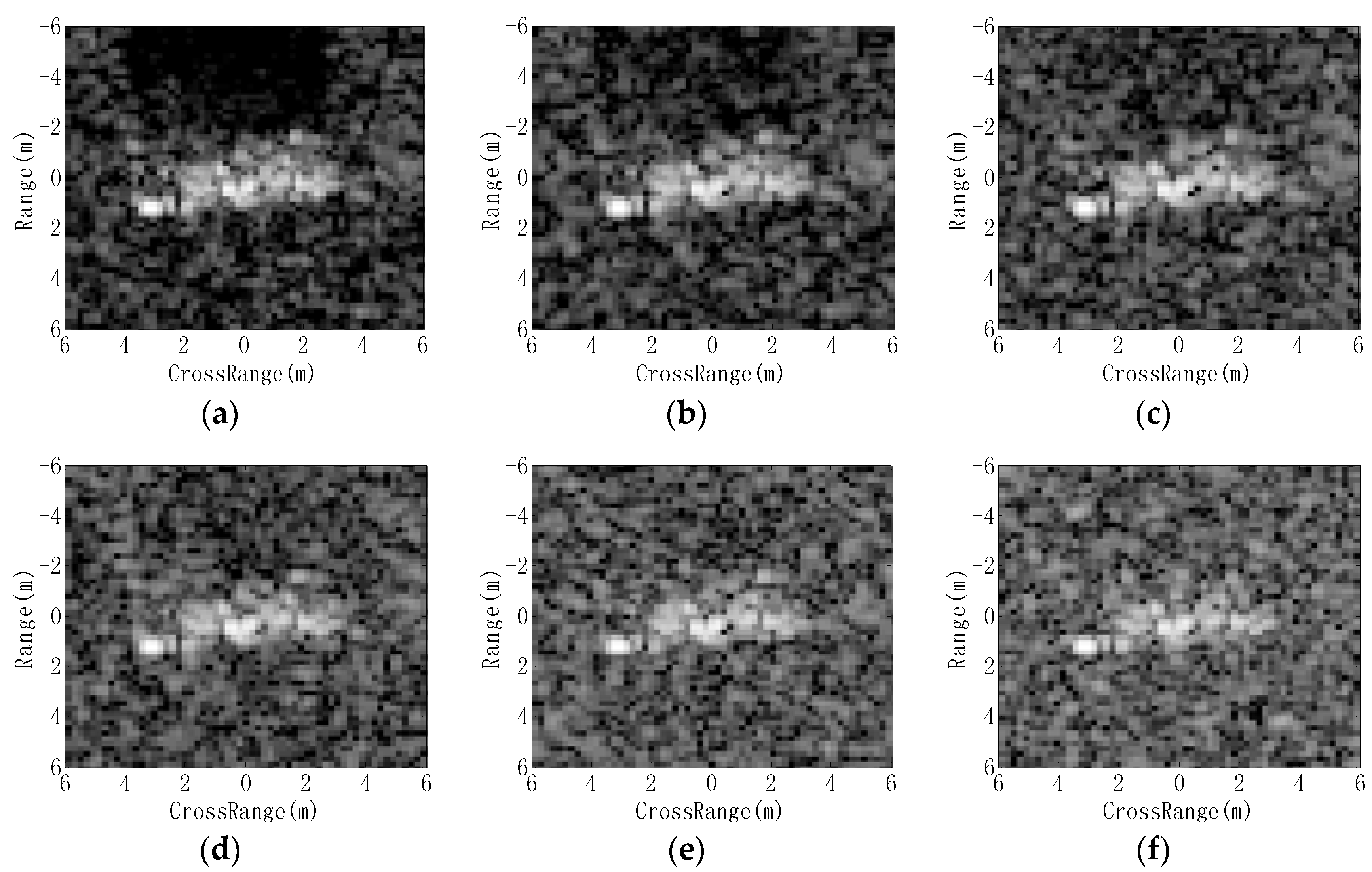
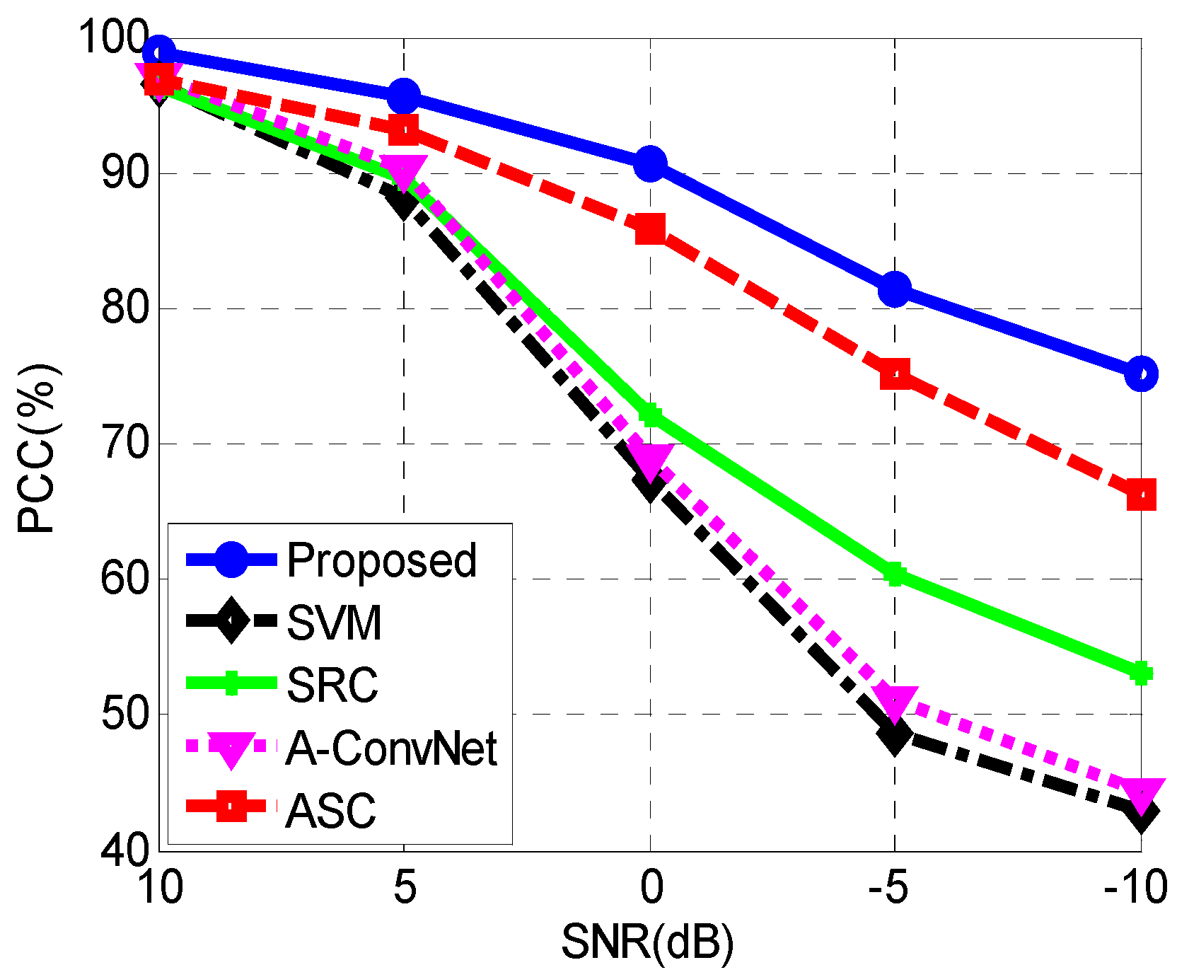
5.3.3. Noise Corruption

The test images collected in the real-world scenarios are often contaminated by the noises from the background environment or radar systems. Hence, it is crucial that the recognition algorithms can maintain robust under possible noise corruption. To test the performance of the proposed method under noise corruption, the noisy SAR images are first simulated by adding additive Gaussian noises to the original images according to the predefined signal-to-noise ratio (SNR) [48]. Figure 9 shows the noisy images at different SNRs. With the deterioration of noise contamination, more and more target characteristics are submerged in the noises, which will definitely increase the difficulty of correct target recognition.

Figure 10 plots the average PCCs of different methods under noise corruption. In comparison, the proposed method has the best robustness to noise corruption with the highest PCCs at each SNR. The ASC method outperforms SVM, SRC, and CNN at SNRs lower than 5 dB. The reasons can be analyzed from two aspects. On one hand, the ASCs are noise-robust features. Then, the ASCs of noisy images can still be extracted with good precision to match well with those from the template samples. On the other hand, the local variations caused by noise corruption can be better handled via the one-to-one correspondence between two ASC sets. In the proposed method, the ASC matching method can effectively complement the designed CNN to cope with those severely corrupted samples. Therefore, the final performance is significantly improved.

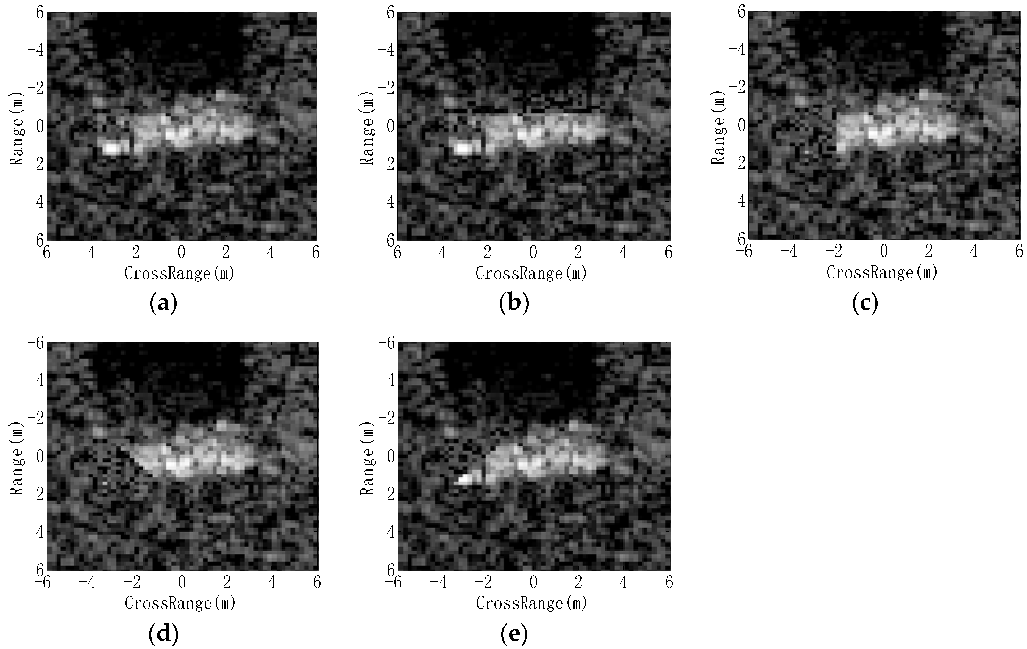
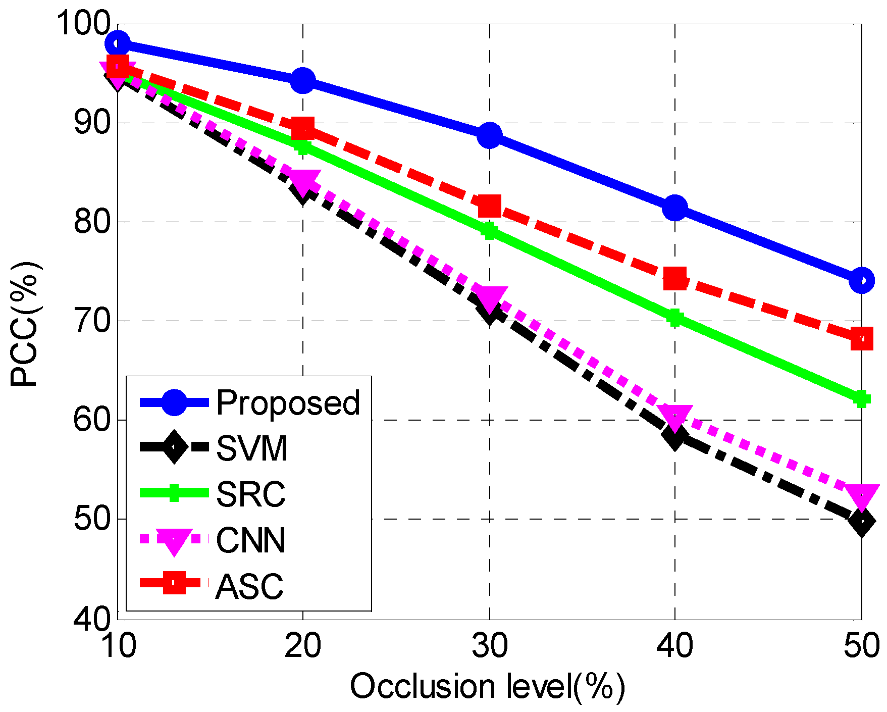
5.3.4. Partial Occlusion

The target may be occluded by the obstacles or camouflaged intentionally. In this case, a part of the target may not be presented in the captured SAR image. According to the SAR occlusion model in [20,49], the partially occluded image is simulated by removing a certain proportion of the target region of the original image from eight directions. Figure 11 shows the 20% occluded SAR images from four different directions whereas the remaining ones are in the symmetrical directions. Figure 12 plots the average PCCs of the eight directions of different methods. With the highest PCC at each occlusion level, the proposed method is validated to be the most robust to partial occlusion. The ASC method outperforms the remaining ones when the occlusion level goes higher than 30%. The main reason is that the stable ASCs in occluded images can still be matched well. For the proposed method, the ASC matching works cooperatively with the CNN to cope with the severely occluded images. Therefore, the fused performance is much better than others.

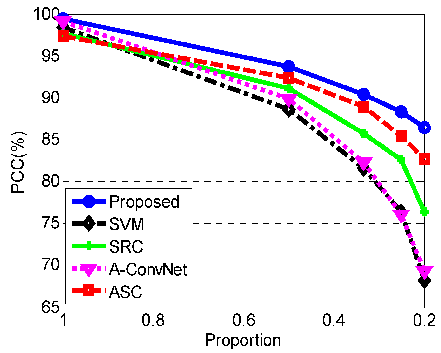
5.4. Limited Training Samples

Actually, the available training resource for SAR ATR is quite limited [37,38]. As a result, the training samples may only cover a certain proportion of the full 360° azimuth range. For experimental evaluation, we randomly select 1/2, 1/3, 1/4, 1/5 and 1/6 from each of the 10-class samples and then perform target recognition based on the reduced training set. As shown in Figure 13, the proposed method keeps the highest PCC at each reduction level, validating its best robustness to limited training samples. In addition, ASC method shares an approaching performance to the proposal and outperforms the remaining ones significantly. For SVM, SRC and CNN, their performances are closely related to the completeness of the training set. When the training samples are reduced severely, their PCCs experience sharp decreases. In the ASC method, the corresponding templates are selected based on the azimuth of the test image. In fact, the ASCs can maintain stable in a certain azimuth interval (e.g., [−5°, 5°]) [50]. Then, the ASC matching can still be performed with good effectiveness. As a combination of CNN and ASC matching, the proposed method achieves the best performance mainly by inheriting the robustness of ASC matching.

6. Discussion

The experimental results based on the MSTAR dataset validate the superior effectiveness and robustness of the proposed method under SOC and several EOCs compared with several state-of-the-art SAR ATR methods including SVM, SRC, A-ConvNet and ASC matching method. In detail, the reasonability lay behind the experimental results is discussed as follows.

(i)

Experiment under SOC. Under SOC, the training and test samples are notably similar with only a 2° depression angle difference. Consequently, all the methods achieve very high PCCs. Due to the powerful classification capability of CNN under SOC, most test samples are actually classified by CNN in the proposed method. The remaining ones can also be effectively classified by ASC matching because of its goof performance. Hence, the hierarchical fusion of the two classification schemes can maintain the excellent performance under SOC, which is demonstrated to outperform the others. In this case, the excellent performance of the proposed method mainly benefits from CNN. Meanwhile, ASC matching further improves the recognition performance by handling a few test samples, which possibly have many differences with the training ones.

(ii)

Experiment under EOCs. The EOCs like configuration variance, depression angle variance, noise corruption and partial occlusion probably cause some local variations of the target in the test SAR images. Therefore, the one-to-one correspondence between the local descriptors, i.e., ASCs, can better handle these situations. For the classifiers like SVM, SRC and CNN, the training samples only include SAR images of intact targets with high SNRs. In addition, only a specific configuration is bracketed. Therefore, their performances degrade greatly under these EOCs. In the proposed method, when a test sample cannot be reliably classified by CNN, ASC matching can probably provide a correct decision. Therefore, via hierarchically fusing CNN and ASC matching, the robustness of the proposed method can be enhanced. In this case, the superior robustness of the proposed method mainly benefits from the merits of ASC matching. However, for those EOCs which are not severely different from the training set (e.g., small amount of noise additions), CNN is probable to make correct decisions on them. Therefore, CNN can complement ASC matching to further improve ATR performance.

(iii)

Experiment under limited training samples. With limited training samples, the classification capabilities of SVM, SRC and CNN will be impaired greatly. For the ASC matching method, the template ASCs still share a high correlation with the test ASCs because the stability of ASCs can be maintained in a certain azimuth interval. Therefore, once the CNN cannot form a reliable decision for the test image, the ASC matching can better cope with the situation.

All in all, in this study, CNN is adopted as the basic classifier, which can operate with high effectiveness and efficiency when the test sample is covered by the training set. As a complement to CNN, the test samples that are severely corrupted by EOCs and can hardly be determined by CNN are further identified by ASC matching. The detailed analysis between two ASC sets helps make correction decisions for various EOCs. Therefore, the hierarchical fusion of the two classification schemes notably promotes the final ATR performance.

The future works can be conducted from two aspects. On one hand, the specific architecture of CNN for SAR ATR should be studied to further improve the recognition performance. At present stage, the CNNs for SAR ATR are mainly introduced from the field of optical image processing. The specific network for SAR image interpretation should be further researched. On the other hand, more efficient and robust classier can be incorporated into the proposed framework to further enhance the robustness of the ATR system. ASC matching is a representative of local classifier, which performs target recognition by analyzing the local variations of the target. It may exist other similar classification schemes, which can further improve the robustness of SAR ATR.

7. Conclusions

A SAR ATR method by hierarchically fusing CNN and ASC matching is proposed in this study. A test sample is first classified by CNN. When there is no reliable decision, it will be further recognized by ASC matching. CNN can achieve notably high classification accuracy under SOC, when the test samples are covered by the training set. ASC matching can better cope with various EOCs related to the local variations of the target such as configuration variance, noise corruption, partial occlusion, etc. Therefore, the hierarchical fusion effectively inherits the high effectiveness of CNN under SOC and good robustness of ASC matching to various EOCs. Extensive experiments are conducted on the MSTAR dataset under SOC and typical EOCs including configuration variance, depression angle variance, noise corruption and partial occlusion. Based on the experimental results, several conclusions can be drawn as follows.

(i)

CNN has powerful classification capability under SOC. Thus, it is a reasonable choice to use is as the basic classifier. In addition, ASC matching can also work very well under SOC because of the good discrimination of ASCs. Therefore, the hierarchical fusion of the two classification schemes can maintain excellent performance under SOC.

(ii)

ASC matching can achieve very good robustness under different types of EOCs. The one-to-one correspondence between two ASC sets can sense the local variations of the target thus the resulted similarity measure can better handle these situations. Therefore, those samples which cannot be reliably classified by CNN are probably to obtain correct decisions by ASC matching.

(iii)

The proposed method achieves the best performance under both SOC and EOCs compared with other state-of-the-art methods by combining the merits of the two classification schemes.

In conclusion, the proposed method has much potential to improve the ATR performance in practical applications.

References

1. Xu, Z.; Chen, K.S. On signal modeling of moon-based synthetic aperture radar (SAR) imaging of earth. Remote Sens. 2018, 10, 486. [Google Scholar] [CrossRef]
2. Ao, D.Y.; Wang, R.; Hu, C.; Li, Y.H. A sparse SAR imaging method based on multiple measurement vectors model. Remote Sens. 2017, 9, 297. [Google Scholar] [CrossRef]
3. Cumming, I.G.; Wong, F.H. Digital Processing of Synthetic Aperture radar Data: Algorithms and Implementation; Artech House: London, UK, 2004; ISBN 978-7-121-16977-9. [Google Scholar]
4. Argenti, F.; Lapini, A.; Bianchi, T.; Alparone, L. A tutorial on speckle reduction in synthetic aperture radar Images. IEEE Geosci. Remote Sens. Mag. 2013, 1, 6–35. [Google Scholar] [CrossRef]
5. El-Darymli, K.; Gill, E.W.; McGuire, P.; Power, D.; Moloney, C. Automatic target recognition in synthetic aperture radar imagery: A state-of-the-art review. IEEE Access 2016, 4, 6014–6058. [Google Scholar] [CrossRef]
6. El-Darymli, K.; McGuire, P.; Power, D.; Moloney, C. Target detection in synthetic aperture radar imagery: A state-of-the-art survey. J. Appl. Remote Sens. 2013, 13, 071598. [Google Scholar] [CrossRef]
7. Gao, G. An improved scheme for target discrimination in high-resolution SAR images. IEEE Trans. Geosci. Remote Sens. 2011, 49, 277–294. [Google Scholar] [CrossRef]
8. Ding, B.Y.; Wen, G.J.; Ma, C.H.; Yang, X.L. Target recognition in synthetic aperture radar images using binary morphological operations. J. Appl. Remote Sens. 2016, 10, 046006. [Google Scholar] [CrossRef]
9. Amoon, M.; Rezai-rad, G. Automatic target recognition of synthetic aperture radar (SAR) images based on optimal selection of Zernike moment features. IET Comput. Vis. 2014, 8, 77–85. [Google Scholar] [CrossRef]
10. Park, J.; Park, S.; Kim, K. New discrimination features for SAR automatic target recognition. IEEE Geosci. Remote Sens. Lett. 2013, 10, 476–480. [Google Scholar] [CrossRef]
11. Anagnostopulos, G.C. SVM-based target recognition from synthetic aperture radar images using target region outline descriptors. Nonlinear Anal. 2009, 71, e2934–e2939. [Google Scholar] [CrossRef]
12. Papson, S.; Narayanan, R.M. Classification via the shadow region in SAR imagery. IEEE Trans. Aerosp. Electron. Syst. 2012, 48, 969–980. [Google Scholar] [CrossRef]
13. Cui, J.J.; Gudnason, J.; Brookes, M. Automatic recognition of MSTAR targets using radar shadow and super resolution features for. In Proceedings of the IEEE International Conference on Acoustics, Speech, and Signal Processing (ICASSP), Philadelphia, PA, USA, 18–23 March 2005. [Google Scholar]
14. Mishra, A.K. Validation of PCA and LDA for SAR ATR. In Proceedings of the 2008 IEEE Region 10 Conference, Hyderabad, India, 19–21 November 2008; pp. 1–6. [Google Scholar]
15. Cui, Z.Y.; Cao, Z.J.; Yang, J.Y.; Feng, J.L.; Ren, H.L. Target recognition in synthetic aperture radar via non-negative matrix factorization. IET Radar Sonar Navig. 2015, 9, 1376–1385. [Google Scholar] [CrossRef]
16. Huang, Y.L.; Pei, J.F.; Yang, J.Y.; Liu, X. Neighborhood geometric center scaling embedding for SAR ATR. IEEE Trans. Aerosp. Electron. Syst. 2014, 50, 180–192. [Google Scholar] [CrossRef]
17. Yu, M.T.; Dong, G.G.; Fan, H.Y.; Kuang, G.Y. SAR target recognition via local sparse representation of multi-manifold regularized low-rank approximation. Remote Sens. 2018, 10, 211. [Google Scholar]
18. Gerry, M.J.; Potter, L.C.; Gupta, I.J.; Merwe, A. A parametric model for synthetic aperture radar measurement. IEEE Trans. Antennas Propag. 1999, 47, 1179–1188. [Google Scholar] [CrossRef]
19. Potter, L.C.; Mose, R.L. Attributed scattering centers for SAR ATR. IEEE Trans. Image Process. 1997, 6, 79–91. [Google Scholar] [CrossRef] [PubMed]
20. Bhanu, B.; Lin, Y. Stochastic models for recognition of occluded targets. Pattern Recognit. 2003, 36, 2855–2873. [Google Scholar] [CrossRef]
21. Chiang, H.; Moses, R.L.; Potter, L.C. Model-based classification of radar images. IEEE Trans. Inf. Theory 2000, 46, 1842–1854. [Google Scholar] [CrossRef]
22. Ding, B.Y.; Wen, G.J.; Huang, X.H.; Ma, C.H.; Yang, X.L. Target recognition in synthetic aperture radar images via matching of attributed scattering centers. IEEE J. Sel. Top. Appl. Earth Obs. Remote Sens. 2017, 10, 3334–3347. [Google Scholar] [CrossRef]
23. Ding, B.Y.; Wen, G.J.; Zhong, J.R.; Ma, C.H.; Yang, X.L. A robust similarity measure for attributed scattering center sets with application to SAR ATR. Neurocomputing 2017, 219, 130–143. [Google Scholar] [CrossRef]
24. Ding, B.Y.; Wen, G.J.; Zhong, J.R.; Ma, C.H.; Yang, X.L. Robust method for the matching of attributed scattering centers with application to synthetic aperture radar automatic target recognition. J. Appl. Remote Sens. 2016, 10, 016010. [Google Scholar] [CrossRef]
25. Ding, B.Y.; Wen, G.J.; Huang, X.H.; Ma, C.H.; Yang, X.L. Data augmentation by multilevel reconstruction using attributed scattering center for SAR target recognition. IEEE Geosci. Remote Sens. Lett. 2017, 14, 979–983. [Google Scholar] [CrossRef]
26. Zhou, J.X.; Shi, Z.G.; Cheng, X.; Fu, Q. Automatic target recognition of SAR images based on global scattering center model. IEEE Trans. Geosci. Remote Sens. 2011, 49, 3713–3729. [Google Scholar]
27. Ding, B.Y.; Wen, G.J. A region matching approach based on 3-D scattering center model with application to SAR target recognition. IEEE Sens. J. 2018, 18, 4623–4632. [Google Scholar] [CrossRef]
28. Sun, Y.J.; Liu, Z.P.; Todorovic, S.; Li, J. Adaptive boosting for SAR automatic target recognition. IEEE Trans. Aerosp. Electron. Syst. 2007, 43, 112–125. [Google Scholar] [CrossRef]
29. Srinivas, U.; Monga, V.; Raj, R.G. SAR automatic target recognition using discriminative graphical models. IEEE Trans. Aerosp. Electron. Syst. 2014, 50, 591–606. [Google Scholar] [CrossRef]
30. Zhao, Q.; Principe, J.C. Support vector machines for synthetic radar automatic target recognition. IEEE Trans. Aerosp. Electron. Syst. 2001, 37, 643–654. [Google Scholar] [CrossRef]
31. Liu, H.C.; Li, S.T. Decision fusion of sparse representation and support vector machine for SAR image target recognition. Neurocomputing 2013, 113, 97–104. [Google Scholar] [CrossRef]
32. Song, H.B.; Ji, K.F.; Zhang, Y.S.; Xing, X.W.; Zou, H.X. Sparse representation-based SAR image target classification on the 10-class MSTAR data set. Appl. Sci. 2016, 6, 26. [Google Scholar] [CrossRef]
33. Thiagarajan, J.; Ramamurthy, K.; Knee, P.P.; Spanias, A.; Berisha, V. Sparse representation for automatic target classification in SAR images. In Proceedings of the 2010 4th Communications, Control and Signal Processing (ISCCSP), Limassol, Cyprus, 3–5 March 2010. [Google Scholar]
34. Krizhevsky, A.; Sutskever, I.; Hinton, G.E. Imagenet classification with deep convolutional neural networks. In Proceedings of the Neural Information Processing System (NIPS), Harrahs and Harveys, Lake Tahoe, NV, USA, 3–8 December 2012; Volume 2, pp. 1096–1105. [Google Scholar]
35. Szegedu, C.; Liu, W.; Jia, Y.; Sermanet, P.; Reed, S.; Anguelov, D.L.; Erhan, D.; Vanhoucke, V.; Rabinovich, A. Going deeper with convolutions. In Proceedings of the IEEE Conference on Computer Vision and Pattern Recognition (CVPR), Boston, MA, USA, 7–12 June 2015; pp. 1–9. [Google Scholar]
36. He, K.; Zhang, X.; Ren, S.; Sun, J. Deep residual learning for image recognition. In Proceedings of the IEEE Conference on Computer Vision and Pattern Recognition (CVPR), Las Vegas, NV, USA, 17–30 June 2016; pp. 770–778. [Google Scholar]
37. Dong, G.G.; Kuang, G.Y.; Wang, N.; Zhao, L.J.; Lu, J. SAR target recognition via joint sparse representation of monogenic signal. IEEE J. Sel. Top. Appl. Earth Obs. Remote Sens. 2015, 8, 3316–3328. [Google Scholar] [CrossRef]
38. Ding, B.Y.; Wen, G.J. Sparsity constraint nearest subspace classifier for target recognition of SAR images. J. Vis. Commun. Image Represent. 2018, 52, 170–176. [Google Scholar] [CrossRef]
39. Chen, S.Z.; Wang, H.P.; Xu, F.; Jin, Y.Q. Target classification using the deep convolutional networks for SAR images. IEEE Trans. Geosci. Remote Sens. 2016, 47, 1685–1697. [Google Scholar] [CrossRef]
40. Furukawa, H. Deep learning for target classification from SAR imagery: Data augmentation and translation invariance. arXiv, 2017; arXiv:1708.07920. [Google Scholar]
41. Ding, J.; Chen, B.; Liu, H.W.; Huang, M.Y. Convolutional neural network with data augmentation for SAR target recognition. IEEE Geosci. Remote Sens. Lett. 2016, 13, 364–368. [Google Scholar] [CrossRef]
42. Du, K.N.; Deng, Y.K.; Wang, R.; Zhao, T.; Li, N. SAR ATR based on displacement- and rotation- insensitive CNN. Remote Sens. Lett. 2016, 7, 895–904. [Google Scholar] [CrossRef]
43. Demetrios, G.; Nikou, C.; Likas, A. Registering sets of points using Bayesian regression. Neurocomputing 2013, 89, 122–133. [Google Scholar]
44. Liu, H.W.; Jiu, B.; Li, F.; Wang, Y.H. Attributed scattering center extraction algorithm based on sparse representation with dictionary refinement. IEEE Trans. Antennas Propag. 2017, 65, 2604–2614. [Google Scholar] [CrossRef]
45. Cong, Y.L.; Chen, B.; Liu, H.W.; Jiu, B. Nonparametric Bayesian attributed scattering center extraction for synthetic aperture radar targets. IEEE Trans. Signal Process. 2016, 64, 4723–4736. [Google Scholar] [CrossRef]
46. Ding, B.Y.; Wen, G.J. Target recognition of SAR images multi-resolution representaion. Remote Sens. Lett. 2017, 8, 1006–1014. [Google Scholar] [CrossRef]
47. Ravichandran, B.; Gandhe, A.; Simith, R.; Mehra, R. Robust automatic target recognition using learning classifier systems. Inf. Fusion 2007, 8, 252–265. [Google Scholar] [CrossRef]
48. Doo, S.; Smith, G.; Baker, C. Target classification performance as a function of measurement uncertainty. In Proceedings of the 5th Asia-Pacific Conference on Synthetic Aperture Radar, Singapore, 1–4 September 2015. [Google Scholar]
49. Ding, B.Y.; Wen, G.J. Exploiting multi-view SAR images for robust target recognition. Remote Sens. 2017, 9, 1150. [Google Scholar] [CrossRef]
50. Ding, B.Y.; Wen, G.J.; Huang, X.H.; Ma, C.H.; Yang, X.L. Target recognition in SAR images by exploiting the azimuth sensitivity. Remote Sens. Lett. 2017, 8, 821–830. [Google Scholar] [CrossRef]
Figure 1. Architecture of the proposed CNN.
Remotesensing 10 00819 g001
Figure 2. The training loss versus epoch.
Remotesensing 10 00819 g002
Figure 3. Illustration of the trained CNN.
Remotesensing 10 00819 g003
Figure 4. General procedure of the proposed target recognition method.
Remotesensing 10 00819 g004
Figure 5. Optical images of the ten military targets.
Remotesensing 10 00819 g005
Figure 6. Performance of the proposed method under different thresholds.
Remotesensing 10 00819 g006
Figure 7. Four configurations of T72 tank.
Remotesensing 10 00819 g007
Figure 8. SAR images of 2S1 at different depression angles being. (a) 17°; (b) 30°; (c) 45°.
Remotesensing 10 00819 g008
Figure 9. Noisy images at different SNRs. (a) original image (b) 10 dB (c) 5 dB (d) 0 dB (e) −5 dB (f) −10 dB.
Remotesensing 10 00819 g009
Figure 10. Comparison of different methods under noise corruption.
Remotesensing 10 00819 g010
Figure 11. 20% occluded images from different directions. (a) Original image; (b) direction 1; (c) direction 3; (d) direction 5; (e) direction 7.
Remotesensing 10 00819 g011
Figure 12. Comparison of different methods under partial occlusion.
Remotesensing 10 00819 g012
Figure 13. Comparison of different methods under limited training samples.
Remotesensing 10 00819 g013