Machine Learning Automatic Model Selection Algorithm for Oceanic Chlorophyll-a Content Retrieval

Abstract

Ocean Color remote sensing has a great importance in monitoring of aquatic environments. The number of optical imaging sensors onboard satellites has been increasing in the past decades, allowing to retrieve information about various water quality parameters of the world’s oceans and inland waters. This is done by using various regression algorithms to retrieve water quality parameters from remotely sensed multi-spectral data for the given sensor and environment. There is a great number of such algorithms for estimating water quality parameters with different performances. Hence, choosing the most suitable model for a given purpose can be challenging. This is especially the fact for optically complex aquatic environments. In this paper, we present a concept to an Automatic Model Selection Algorithm (AMSA) aiming at determining the best model for a given matchup dataset. AMSA automatically chooses between regression models to estimate the parameter in interest. AMSA also determines the number and combination of features to use in order to obtain the best model. We show how AMSA can be built for a certain application. The example AMSA we present here is designed to estimate oceanic Chlorophyll-a for global and optically complex waters by using four Machine Learning (ML) feature ranking methods and three ML regression models. We use a synthetic and two real matchup datasets to find the best models. Finally, we use two images from optically complex waters to illustrate the predictive power of the best models. Our results indicate that AMSA has a great potential to be used for operational purposes. It can be a useful objective tool for finding the most suitable model for a given sensor, water quality parameter and environment.

1. Introduction

Ocean Color (OC) monitoring from spaceborne and airborne platforms using remote sensing techniques has been receiving an increased focus in the past decades [1,2]. This is due to the fact that an ever-increasing amount of remote sensing data is getting available, but also, because of increased anthropogenic activity and climate change have resulted in changes in the water quality [3]. Coastal waters are one of the most sensitive areas due to their vulnerable ecosystems. Worsened water quality might endanger these ecosystems (such as fish’s habitats [4]), which has both economical and ecological importance [3]. It is well-known that the eutrophication of coastal waters and inland waters has been increasing lately, leading to decreased water-quality [5,6]. Continuously monitoring of the water-bodies, with special focus to coastal waters is therefore important for various reasons. It can also contribute to improved understanding of the ongoing changes, and the impact of increased anthropogenic activities on the ecosystems [7].

The quality of water bodies, both globally and regionally, is most efficiently inferred from color using multi-spectral or hyper-spectral remote sensing. The color of the oceans is determined by the different type, amount and distribution of water constituents. Being able to monitor these water constituents allows to retrieve information about the environmental state of the water [8]. The most common parameters used for monitoring water quality are Chlorophyll-a (Chl-a), Colored Dissolved Organic Matter (CDOM), Total Suspended Matter (TSM), Secchi Disk Depth (SDD), turbidity, Total Phosphorus (TP), to name some [3].

However, the retrieval of water quality contents from remote sensing data is not always strait forward. Algorithms are generally dependent on the sensors’ characteristics, geographical location, and environmental conditions of the water body. The objective of this paper is to present and demonstrate a strategy for an Automatic Model Selection Algorithm (AMSA), for retrieval of water quality parameters from remote sensing data, given an appropriate matchup dataset. Since Chl-a is one of the most important and most studied of these water quality parameters [5], we will use Chl-a as an example parameter throughout the paper. Besides, estimating aquatic Chl-a concentration has several important applications, in addition to providing information about water-quality. Chl-a occurs in phytoplankton in aquatic environments. Phytoplankton uses photosynthesis in order to live and grow. Capturing of light, which is the driving of photosynthesis [9], takes place in the Chl-a molecule. Estimating Chl-a content allows to retrieve information about the aquatic biomass and several biophysical processes. During photosynthesis, phytoplankton takes up Carbon-Dioxid (CO${}_2$) [10]. Therefore, monitoring phytoplankton through Chl-a might also contribute to the understanding of climate change [11,12,13].

Using Chl-a as an example, we will in the following give some rational and motivation for AMSA. Remote sensing of Chl-a content (and other water quality parameters) is done by optical imaging sensors onboard satellites, which have different spectral and spatial resolutions. Chl-a content is usually retrieved by relating the measured signal at the sensor, the remote sensing reflectance (Rrs), to coincident in-water Chl-a measurements (see for instance the National Aeronautics and Space Administration’s (NASA) OC products [14,15,16,17,18]). This dataset is denoted a so-called matchup dataset, and forms the basis for most of the algorithms used for Chl-a content estimation from remotely sensed data. Since the various sensors have different number of bands at different central wavelengths (see Table 2), the matchup data has to be calibrated for each given sensor.

Furthermore, there are a manifold of retrieval algorithms available to the user [19,20,21]. Some of them are designed to estimate Chl-a globally, whereas others are region specific. These algorithms are in general sensor specific, this means they require a new or adjusted model for each sensor. For an untrained user, it is often challenging to establish or choose the most suitable Chl-a retrieval model. This is especially the fact for optically challenging aquatic environments, such as coastal waters [22]. Coastal waters are often dominated by other water constituents than Chl-a, such as CDOM, and CDOM and Chl-a are known to have their absorption peak in the same spectral region. This results in difficulties in distinguishing between the signals originating from Chl-a and CDOM, especially, when Chl-a content is estimated by algorithms that use the absorption peak of the Chl-a molecule.

As more datasets are collected, and computer processing power gets unlimited, machine learning (ML) algorithms have become more feasible in OC applications. ML models are not based on assumption about the Chl-a absorption spectrum. They learn the relationship between the in-situ Chl-a content and the available Rrs values, and use this learned functional relationship for prediction. These models use all the available spectral bands for learning and prediction, which results that the importance of the spectral bands in the regression process is kept hidden. It can be questioned whether all the bands are needed to obtain the best regression for a given model and region. Artificial Neural Networks (ANN) models have been lately successfully applied for Chl-a estimation [23,24,25], and to various other applications, such as for predicting the amount of generated electricity [26], suspendid sediment load in rivers [27] and rainfall and runoff predictions ahead in time [28]. For OC applications, satellite derived Chl-a in optically complex waters is also often estimated by using other ML algorithms [29,30,31,32].

Furthermore, complex waters show great regional variations, which leads to erroneous Chl-a estimates, when algorithms tuned on global datasets, are applied to a local region [19]. Therefore, it is often required to design local algorithms, which are trained on datasets from the given region [33,34]. However, choosing the most suitable model for a given region can still be challenging.

The above arguments suggest that an automatic model selection approach could be an important tool in choosing the optimum model to monitor a given aquatic environment. Comparisons of models for various OC applications have been carried out in [35,36,37], but to the best of our knowledge, a flexible and automatized model selection tool for OC application has not yet been proposed in the literature. Being able to objectively compare models and determine the most suitable one for the given data and purpose might be beneficial for the users.

The contribution of this paper is to present a strategy for an Automatic Model Selection Algorithm (AMSA), which outputs the most suitable water quality retrieval model, given the matchup dataset. The current AMSA model uses three ML models as input options. ML models usually rely on feature selection in prior to regression [38]. This is due to the fact that dimensionality reduction is often required to increase accuracy, robustness and computational time [39]. Using feature selection also helps to correctly interpret the data. The method for choosing the most optimal number and combination of features for the given model is model dependent, and needs to be developed in each case. AMSA uses feature ranking methods to assign relevance to the features, then it evaluates the number and combination of these ranked features in regression models using some quantitative regression performance measures.

Hence, AMSA is not only using feature selection prior to regression, but also feature ranking methods derived from regression models based on different principles. This means that the importance of the features is first determined by using several feature ranking approaches, one tailored to each regression model, then sequential forward selection is applied for comparison. Then the regression models are compared by computing regression performance measures. Finally, AMSA returns the best model for the given matchup dataset. Hence, AMSA is neither limited to a given water quality parameter nor to a feature ranking method/regression model/regression performance measure. The only input that it requires, is the matchup dataset.

For demonstration of the performance of AMSA, we use three sophisticated ML models for feature ranking and regression. These regression models are the Gaussian Process Regression (GPR), Support Vector Regression (SVR) and Partial Least Square Regression (PLSR) models. GPR has been shown to outperform empirical [31,40] and ML regression models [41] for biophysical parameter retrieval from remotely sensed data. GPR has several advantageous properties besides its excellent regression performance, for instance the certainty level of the estimates and the possibility to access feature relevance. Feature relevance for the GPR model can be accessed by the Sensitivity Analysis (SA) [31,32] and the Automatic Relevance Determination (ARD) [40,42] feature ranking methods.

The SVR model has also been shown to perform well for OC applications [29,43,44]. In this work, we applied the SA to the SVR model in order to access feature relevance. For classification in neuroimage applications, this has been done in [45]. Here, we introduced the methodology for regression in Chl-a content estimation.

The PLSR model was included in AMSA, because of the Variable Importance in Projection (VIP) feature ranking methods associated with it. PLSR is a strong regression model, which can handle high dimensional inputs, reduce noise and co-linearity in the data [46]. The PLSR model has been applied for OC applications in optically complex aquatic environments [47].

We have previously studied the SA of the GPR model, ARD and VIP feature ranking methods and the GPR and PLSR regression models for Chl-a content estimation in [32]. In [32], we used a MERIS matchup dataset and two additional matchups for the MODIS-Aqua and SeaWiFS sensors to evaluate the methodologies, and concluded that these feature ranking methods can be used to reduce the number of features, while still obtaining comparable estimates for Chl-a content, compared to the state-of-art algorithms.

In the current demonstration of AMSA, we show how the proposed strategy can be used to determine automatically a model for oceanic Chl-a content estimation for both global waters and optically complex waters. The matchup datasets we have used here include a synthetic dataset produced by the International Ocean-Colour Coordinating Group (IOCCG dataset) [48], plus two additional matchups, one for the MERIS sensor (MEdium Resolution Imaging Spectrometer) and one for the MODIS-Aqua (MODerate-resolution Imaging Spectroradiometer) sensor. The IOCCG dataset provides the possibility to threshold the data based on the absorption of the CDOM, and the amount of Chl-a concentrations. Hence, observations which are more likely to occur in complex aquatic environments, can be selected. Furthermore, we resample the IOCCG dataset to match the spectral resolution of the MERIS and MODIS-Aqua matchups.

An additional contribution of this work, is to further extend the feature ranking methods by the sensitivity analysis of the SVR model, which allows us to include the SVR regression model in the AMSA model library. We choose to use the IOCCG dataset to have better control over the optical properties of observations, and include the two matchups for the MERIS and MODIS-Aqua sensors to show that the approach work well on different data sets and for different environmental situations. We highlight that the goal here is to show how the AMSA approach can be used to perform an objective comparison and selection of an optimal model for the given dataset, according to the regression criteria used. AMSA automatically performs feature ranking and training and testing of the regression models. Hence, the output model is already validated. Finally, the demonstration includes two images acquired by MERIS over optically complex aquatic areas to visualize the predictions given by the selected optimal AMSA model.

The rest of this work is organized as follows. Section 2 introduces the general concept of the AMSA and explains the ML AMSA for oceanic Chl-a content estimation in details. Furthermore, the datasets used in this study are described. Section 3 presents the results. Section 4 discusses the results and approach, and highlights advantages and disadvantages of the methodology. Finally, Section 5 concludes this paper and outlines future work.

2. Materials and Methods

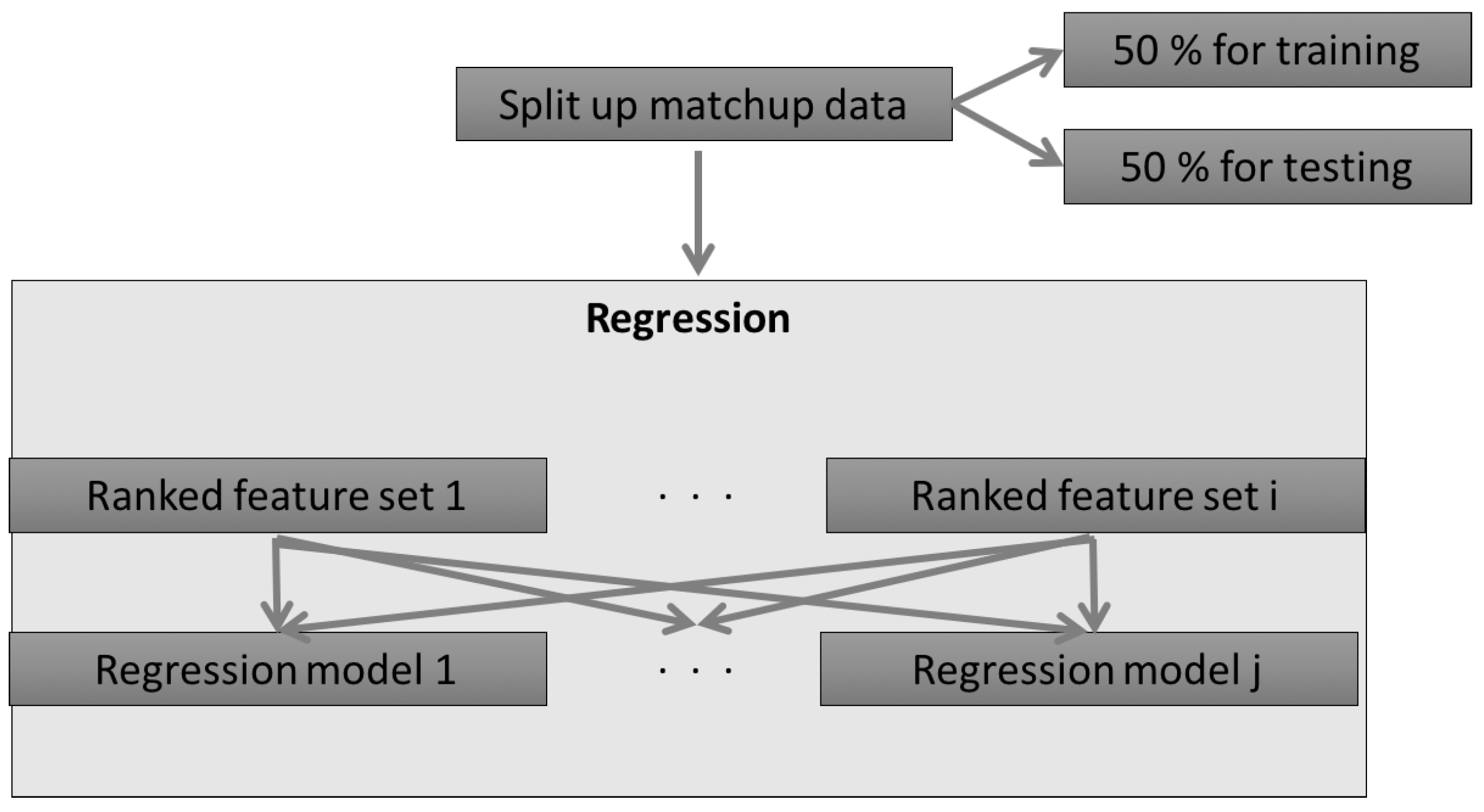
2.1. The Automatic Model Selection Algorithm

2.1.1. The Concept of the AMSA

The AMSA has two stages. In the first stage, relevance is assigned to all the available features by using feature ranking methods. The second stage is to perform regression by using the ranked features as inputs. The best regression model is determined by selecting the most optimal number and combination of features based on the selected goodness of fit criteria. Examples of goodness of fit measures are: Normalized Root Mean Squared Errors (NRMSE) and the Pearson’s correlation coefficient (R${}^2$).

Feature ranking: Assume a matchup dataset D $={\left\{{\mathbf{x}}_n;{\mathbf{y}}_n\right\}}_{n=1}^N$, where ${\mathbf{x}}_n$ is the D dimensional input, D is the number of features, ${\mathbf{y}}_n$ is the corresponding output (ground-truth) and N is the number of measurements. This matchup dataset is used for ranking the D features in $\mathbf{x}$ by using feature ranking methods. Figure 1 shows the feature ranking stage of the algorithm.

The process starts by using all data in the matchup dataset to perform feature ranking. Assume, there are i feature ranking methods. Then the output of this step is i sets of ranked features, each ordered by decreasing relevance (i.e., the first feature in Ranked feature set is the most important, and the last is the least relevant).

Regression and feature selection: Figure 2 and Figure 3 show the flowcharts of the regression stage. In the regression stage, the dataset is split into two parts, 50% is used for training and 50% is used for testing. This partitioning ensures that both training and testing sets contain representative data. Assume j number of Regression models are available. Then an iterative process starts by training and testing Regression model $1,\dots ,j$ with the features in the Ranked feature set $1,\dots ,i$ by using a sequential forward selection approach.

For simplicity, let us assume using Regression model 1 and Ranked feature set 1, containing D ranked features. Regression model 1 starts the training on the training data by taking the most important feature in the Ranked feature set 1. When this model is trained, testing is performed on the test data by computing k Regression performance measures. The results of the computed Regression performance measures are saved (Figure 3).

Then Regression model 1 adds the second most relevant feature of the Ranked feature set 1, in addition to the first one. The system trains and tests the model by computing k Regression performance measures, and saves the results. This procedure continues until the least important feature of the Ranked feature set 1 has been included.

Regression model 1 repeats the same process with all the Ranked feature sets ($1,\dots ,i$). The same procedure is done with all the Regression models ($1,\dots ,j$). The k Regression performance measures are saved for all j Regression models, and for all i Ranked feature sets with all D number of ranked features.

Finally, AMSA searches in the stored Regression performance measures for the model, which resulted in the best performance. AMSA outputs: the best regression model based on the computed regression performance measures; the feature ranking method that resulted the best combination of features associated with the regression model; the number of features, which were needed to obtain the best model; the actual input-features of the best model and also the values of the regression performance measures.

Table 1. The output of the AMSA.

Regression model

Feature ranking method

The features

# of features

Value of the regression performance measures

shows the output of the algorithm.

There are obviously no limitations in the number of feature ranking methods, regression models and regression performance measures to be used in AMSA. Note, if feature ranking is not of interest, this stage can be turned off. In that case, only the most desirable regression model for the given dataset and predefined feature set is returned.

2.2. Demonstration of an AMSA Implementation

The AMSA concept can be used by the users to build an optimal model for her or his application. Any model can be selected, and it can be used for any water quality parameter estimation, as long as matchup data is available. Furthermore, user defined feature ranking methods, regression models and regression performance measures can be included. In this section we present the AMSA we designed for Chl-a estimation. It is based on the work and results presented in [32].

2.2.1. The Matchup Data

We focused on oceanic Chl-a content estimation from Rrs. Hence, the matchup data consists of Rrs measured on the wavelengths of the given sensor and corresponding in-situ Chl-a measurements.

For feature ranking, the complete available dataset was used, while for regression, the dataset was split up in 50% for training and 50% for testing. We chose to split up the data as it follows. The Chl-a values were sorted in an increasing order. The corresponding Rrs values were assigned to the sorted Chl-a values. Then we draw the even numbered observations for forming the training data, and the odd numbered measurements for testing purposes. Hence, both the training and test data was as representative as possible. Note, the way of splitting the data in AMSA can be defined differently. The dataset can be divided randomly and in a different proportion for training and testing, as well.

2.2.2. Regression Models

Assume a dataset consisting of in situ Chl-a values $y_{n=1}^N$ and corresponding input Rrs values ${\{{\mathbf{x}}_n\in R^D\}}_{n=1}^N$, where $n=1,\dots ,N$ is the number of measurements and $d=1,\dots ,D$ is the number of features (spectral bands) for all the regression models. We will use here regression models, namely Gaussian Process Regression, Support Vector Regression and Partial Least Squares Regression. These are briefly summarized below.

Gaussian Process Regression model: The Gaussian Process Regression (GPR) model assumes that the output (Chl-a) is a function of the input (Rrs) and some noise ${\epsilon }_n$, which can be written by $y_n=f\left({\mathbf{x}}_n\right)+{\epsilon }_n$ for $n=1,\dots ,N$, where the noise term is assumed to be additive, independently, identically Gaussian distributed with zero mean and constant variance, i.e., ${\epsilon }_n\sim N(0,{\sigma }^2)$. The model learns this function by fitting a multivariate joint Gaussian distribution over the function values, $f\left({\mathbf{x}}_1\right),\dots ,f\left({\mathbf{x}}_N\right)\sim N(\mathbf{0},\mathbf{K})$, with zero mean and covariance matrix $\mathbf{K}$. Then this can be used for predicting the unseen output Chl-a $y_{\ast }$ for a new input Rrs ${\mathbf{x}}_{\ast }$ by defining a joint prior distribution between the available Chl-a $\mathbf{y}\equiv {\left\{y_n\right\}}_{n=1}^N$ and $y_{\ast }$. This can be mathematically expressed by

$$\left[\begin{array}{c}\mathbf{y}\\ y_{\ast }\end{array}\right]\sim N\left(\mathbf{0},\left[\begin{array}{cc}\mathbf{K}+{\sigma }^2{\mathbf{I}}_n& {\mathbf{k}}_{\ast }\\ {\mathbf{k}}_{\ast }^{\top }& k_{\ast \ast }+{\sigma }^2\end{array}\right]\right),$$

(1)

where ${\mathbf{k}}_{\ast }$ is the covariance between the training vector and the test point, $k_{\ast \ast }$ is the covariance between the test point with itself, and $\mathbf{K}+{\sigma }^2{\mathbf{I}}_n$ is the $N\times N$ noisy covariance matrix of the training inputs. The posterior distribution over the output $y_{\ast }$ can be analytically computed by using Bayes’ formula: $p\left(y_{\ast }\right|{\mathbf{x}}_{\ast },D)=N\left(y_{\ast }\right|{\mu }_{\mathrm{GP}\ast },{\sigma }_{\mathrm{GP}\ast }^2)$, where ${\mu }_{\mathrm{GP}}\ast$ is the predicted Chl-a and ${\sigma }_{\mathrm{GP}\ast }^2$ is the certainty level of the estimated Chl-a content (predictive variance). The predicted Chl-a content can be expressed by ${\mu }_{\mathrm{GP}\ast }={\mathbf{k}}_{\ast }^{\top }{(\mathbf{K}+{\sigma }^2{\mathbf{I}}_n)}^{-1}\mathbf{y}$. Note, the predicted Chl-a content can also be written by ${\mu }_{\mathrm{GP}\ast }={\mathbf{k}}_{\ast }^{\top }\mathbf{\alpha }$, where $\mathbf{\alpha }={(\mathbf{K}+{\sigma }^2{\mathbf{I}}_n)}^{-1}\mathbf{y}$ is the weight vector of the mean function of the GPR model. This allowed the application of the SA (Equation (11)). For further details on the GPR model we refer to [49].

Support Vector Regression model: The Support Vector Regression (SVR) model ([41,50,51,52,53]) estimates Chl-a value from Rrs values by $y_n={\mathbf{w}}^{\mathrm{T}}{\mathbf{x}}_n+b$, where ${\mathbf{w}}^{\mathrm{T}}$ is the transposed weight vector and b is the bias term. The SVR model uses the so-called $ϵ$-intensitive loss function to obtain estimates by penalizing errors exceeding an $ϵ$ limit and at the same time obtaining a regression function as flat as possible. Hence the weights are estimated in the SVR model by minimizing the objective function $J=\frac{1}{\beta }{\sum }_{n=1}^N\left({\zeta }_n^{+}+{\zeta }_n^{-}\right)+\frac{1}{2}{\Vert \mathbf{w}\Vert }^2$ with respect to $\mathbf{w}$, ${\zeta }_n^{+}$, ${\zeta }_n^{-}$ and constrained to

$$\begin{array}{cc}\hfill y_n--{\mathbf{w}}^{\mathrm{T}}{\mathbf{x}}_n--b& \le ϵ+{\zeta }_n^{+}\mathrm{for}n=1,\dots ,N\hfill \end{array}$$

(2)

$$\begin{array}{cc}\hfill {\mathbf{w}}^{\mathrm{T}}{\mathbf{x}}_n+b-y_n& \le ϵ+{\zeta }_n^{-}\mathrm{for}n=1,\dots ,N\hfill \end{array}$$

(3)

$$\begin{array}{cc}\hfill {\zeta }_n^{+},{\zeta }_n^{-}& \ge 0\mathrm{for}n=1,\dots ,N.\hfill \end{array}$$

(4)

${\zeta }_n^{+}$ and ${\zeta }_n^{-}$ are called slack variables, and allow measurements to be larger than $ϵ$, and $\beta >0$ is a constant controlling the trade-off between the flatness of the regression function and the magnitude of the deviations from $ϵ$.

Constructing a Lagrange function from the objective function allows to obtain the optimal solution for the weights: $\widehat{\mathbf{w}}={\sum }_{n=1}^N\left({\alpha }_n^{+}--{\alpha }_n^{-}\right){\mathbf{x}}_n$, where ${\alpha }_n^{+}$ and ${\alpha }_n^{-}$ are the Lagrange multipliers, also referred to as support vectors. Define $a_n={\alpha }_n^{+}--{\alpha }_n^{-}$, and collecting the estimated Chl-a values ${\widehat{y}}_n$ into a vector $\widehat{\mathbf{y}}$, the estimates can be written by

$$\widehat{\mathbf{y}}={\widehat{\mathbf{w}}}^{\mathrm{T}}\mathbf{x}+\widehat{\mathbf{b}}=\sum _{n=1}^N{a}_n{\mathbf{x}}_n^{\mathrm{T}}\mathbf{x}+\widehat{\mathbf{b}}.$$

(5)

Note, that $a_n$ vanishes, when measurements do not exceed $ϵ$, which results that the solution for $\widehat{\mathbf{w}}$ is sparse. Finally, applying the kernel function defined in Equation (13) to ${\mathbf{x}}_n^{\mathrm{T}}\mathbf{x}$, the estimated Chl-a value vector can be expressed by

$$\widehat{\mathbf{y}}=\sum _{n=1}^N{a}_{n}k({\mathbf{x}}_n,\mathbf{x})+\widehat{\mathbf{b}}.$$

(6)

Partial Least Square Regression model: Assume once again the $in-situ$ Chl-a ($\mathbf{X}$) and Rrs ($\mathbf{y}$) training dataset $D\equiv \left\{\mathbf{X},\mathbf{y}\right\}$, where now the observations are collected in matrices, such that $\mathbf{X}$ is an $N\times D$ input data-matrix consisting of $d=1,\dots ,D$ features (spectral bands) and $n=1,\dots ,N$ observations, and let $\mathbf{y}$ be the corresponding $N\times 1$ output-vector (Chl-a measurements), holding $n=1,\dots ,N$ observations.

The Partial Least Square Regression (PLSR) model [46,54] relates the input Rrs $\mathbf{X}$ and the output Chl-a $\mathbf{y}$ through a latent-space. This is done by introducing so-called latent variables $\mathbf{T}$ ($N\times H$), which are representing both $\mathbf{X}$ and $\mathbf{y}$ in the latent-space, such that the covariance between the projection of $\mathbf{X}$ and $\mathbf{y}$ in this latent- space is maximized. The PLSR model can be written by

$$\begin{array}{cc}\hfill \mathbf{X}& =\mathbf{T}{\mathbf{P}}^{\mathrm{T}}+\mathbf{E}\hfill \\ \hfill \mathbf{y}& =\mathbf{T}\mathbf{c}+\mathbf{f}\hfill \\ \hfill \mathbf{T}& =\mathbf{X}{\mathbf{W}}^{\star }\hfill \\ \hfill {\mathbf{W}}^{\star }& =\mathbf{W}{\left({\mathbf{P}}^{\mathrm{T}}\mathbf{W}\right)}^{-1},\hfill \end{array}$$

(7)

where $\mathbf{P}$ ($D\times H$) is a matrix of the X-loadings and $\mathbf{c}$ ($H\times 1$) is the y-loadings, and they are good representations of $\mathbf{X}$ and $\mathbf{y}$, respectively. The term ${\mathbf{W}}^{\star }$ ($D\times H$) holds the weights of $\mathbf{X}$, and defines the common latent-space. The error terms, $\mathbf{E}$ ($N\times D$) and $\mathbf{f}$ ($N\times 1$), are assumed to be iid. $\sim N(0,{\sigma }^2)$. Then we estimate the output Chl-a $\mathbf{y}$ by

$$\mathbf{y}=\mathbf{X}{\mathbf{W}}^{\star }\mathbf{c}+\mathbf{f}=\mathbf{X}\mathbf{b}+\mathbf{f},$$

(8)

where $\mathbf{b}={\mathbf{W}}^{\star }\mathbf{c}$ and $\mathbf{W}$ ($D\times H$) is the weight matrix consisting of the eigenvectors of the variance-covariance matrix ${\mathbf{X}}^{\mathbf{T}}{\mathbf{YY}}^{\mathbf{T}}\mathbf{X}$. Minimizing the error term $\mathbf{f}$ in the PLSR model results the most optimal regression. For further details on the PLSR model and algorithms we refer to [55,56,57,58,59,60].

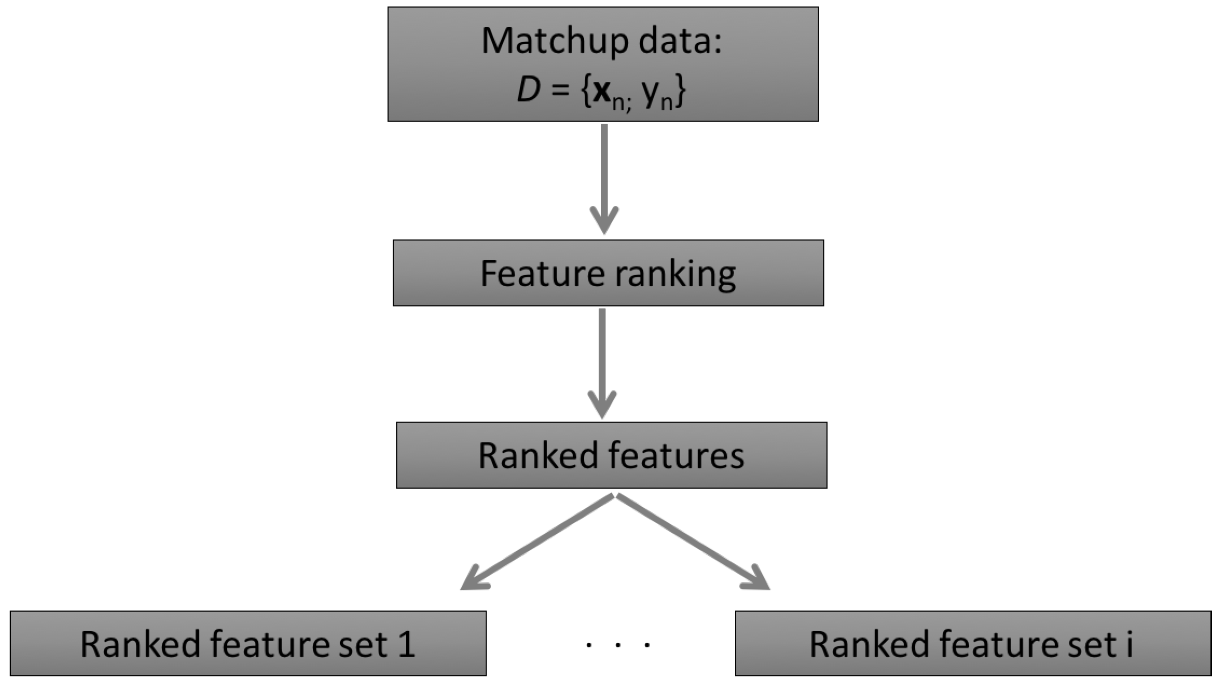
2.2.3. Feature Ranking Methods

We chose four feature ranking methods to assign relevance to the features (in our case spectral bands). The four feature ranking methods are tailored to the regression models, and are the Sensitivity Analysis (SA) of the GPR model, Sensitivity Analysis (SA) of the SVR model, Automatic Relevance Determination (ARD) and Variable Importance in Projection (VIP).

SA of Kernel Machines (GPR and SVR): The SA feature ranking method for the SVR and GPR models are based on the same concept, but for different regression models. Although both the SVR and GPR are non-linear kernel machines, their underlying principles differ. The SA of the GPR model was introduced by [31,61], while the SA of the Support Vector Machine (SVM) for classification purposes was described in [45]. In this work, we extend the SA of the SVM to regression.

Let us define the sensitivity of feature j as

$$s_j=\int {\left({\displaystyle \frac{\partial \mathbf{\varphi }\left(\mathbf{x}\right)}{\partial x_j}}\right)}^{2}p\left(\mathbf{x}\right)\mathrm{d}\mathbf{x},$$

(9)

where $p\left(\mathbf{x}\right)$ is the probability density function of the D-dimensional input vector $\mathbf{x}={[x_1,\dots ,x_D]}^{\top }$, and $\mathbf{\varphi }\left(\mathbf{x}\right)$ represents either the predictive mean function of the GPR model, ${\mu }_{\mathrm{GP}\ast }$ or the estimated output $\widehat{y}$ of the SVR model. The empirical estimate of the sensitivity for the jth feature can be written as

$$s_j={\displaystyle \frac{1}{N}}\sum _{n=1}^N{\left(\frac{\partial \mathbf{\varphi }\left({\mathbf{x}}_n\right)}{\partial x_n^j}\right)}^2,$$

(10)

where N denotes the number of training samples.

Applying the SA (Equation (10)) to the GPR model yields:

$$\begin{array}{cc}\hfill s_{{\mu }_{\mathrm{GP}\star }}^j& ={\displaystyle \frac{1}{N}}\sum _{q=1}^N{\left(\frac{\partial \mathbf{\varphi }\left({\mathbf{x}}_q\right)}{\partial x_q^j}\right)}^2\hfill \\ & ={\displaystyle \frac{1}{N}}\sum _{q=1}^N{\left(\frac{\partial {\sum }_{p=1}^N{\alpha }_{p}k({\mathbf{x}}_p,{\mathbf{x}}_q)}{\partial x_q^j}\right)}^2\hfill \\ & ={\displaystyle \frac{1}{N}}\sum _{q=1}^N{\left(\sum _{p=1}^N\frac{{\alpha }_p(x_p^j-x_q^j)}{{\lambda }_j^2}k({\mathbf{x}}_p,{\mathbf{x}}_q)\right)}^2,\hfill \end{array}$$

(11)

and to the SVR model gives

$$s_{SVR}^j={\displaystyle \frac{1}{N}}\sum _{q=1}^N{\left(\sum _{p=1}^N\frac{a_p(x_p^j-x_q^j)}{{\lambda }_j^2}k({\mathbf{x}}_p,{\mathbf{x}}_q)\right)}^2,$$

(12)

where the difference between Equations (11) and (12) is in the computation of ${\alpha }_p$ and $a_p$ (Note that the calculation of the empirical sensitivity is computed in closed-form using the training data points and the inferred $\mathbf{\alpha }$ and $\mathbf{a}$).

ARD: Kernel Machines (GPR and SVR) use kernel functions to perform regression. The Squared Exponential (SE) kernel function is a widely used kernel function due to its advantageous properties, such as it has infinite derivatives and it is a universal kernel [62]. The SE kernel function can be written by

$$k({\mathbf{x}}_p,{\mathbf{x}}_q)={\nu }^{2}exp\left(-\frac{1}{2}\sum _{d=1}^D{\left({\displaystyle \frac{x_p^d-x_q^d}{{\lambda }_d}}\right)}^2\right),$$

(13)

where ${\lambda }_d$ is the length-scale for feature d, $\nu$ is the positive scale factor and ${\sigma }^2$ is the noise variance. The SE kernel also provides the possibility to access feature relevance. This can be achieved though the optimized length-scale hyperparameters in Equation (13) [40]. Small values of the length-scales indicate greater relevance, while larger values suggest less important features. Hence, the inverses of the optimized length-scale parameters allow the ranking of the features used in the SVR and GPR model.

VIP: The VIP feature ranking method is derived from the Partial Least Squares Regression (PLSR) model. VIP measures the contribution to the total variance of the jth input feature ($j=1,\dots ,D$) [63,64]. The VIP can be written by [65]

$${\mathrm{VIP}}_j=\sqrt{D{\displaystyle \sum _{h=1}^H}S{S}_h(w_{hj}/\parallel w_j{\parallel }^2)/{\displaystyle \sum _{h=1}^H}S{S}_h},$$

(14)

where $S{S}_h$ is the percentage of the output (Chl-a) explained by the so-called hth latent variable and $w_j$ are the weights of the PLSR model.

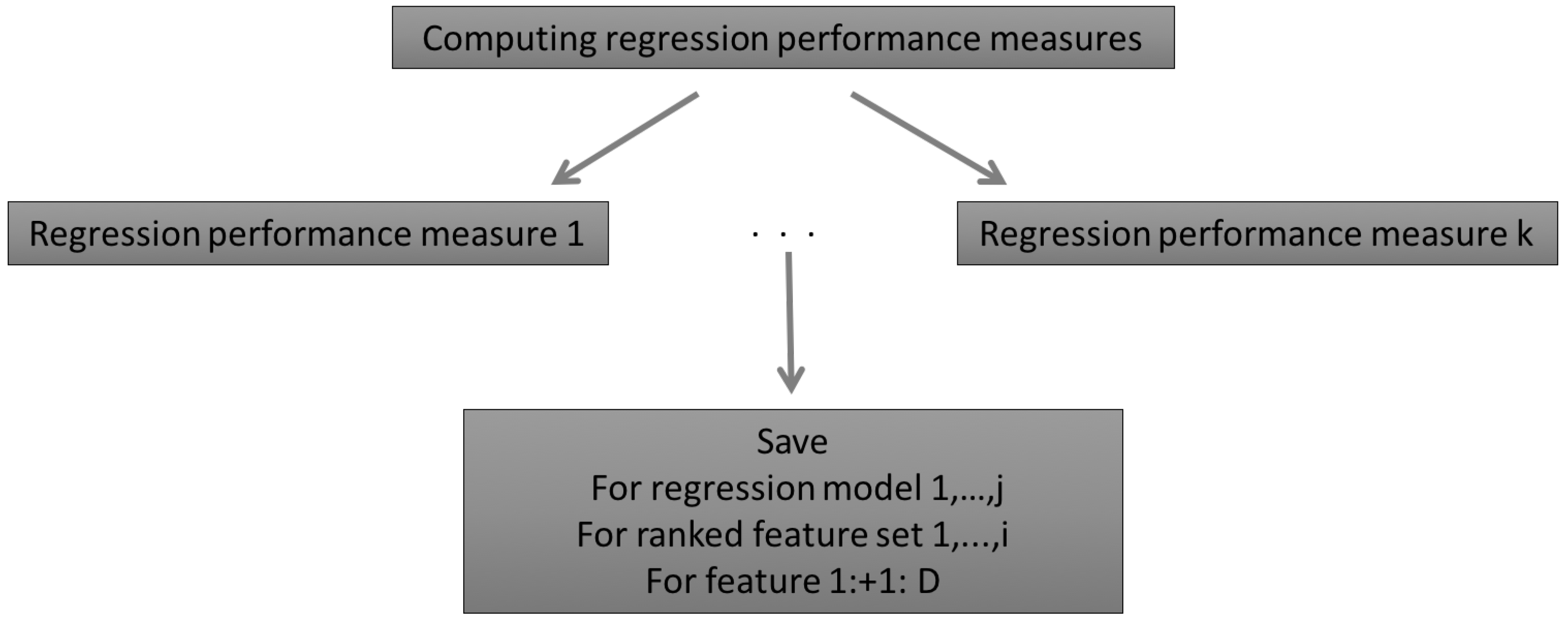
2.2.4. Regression Performance Measures

We chose the Normalized Root Mean Squared Errors (NRMSE) and the Squared Correlation Coefficient (R${}^2$) to evaluate regression strength. These measures are frequently used for model evaluation in remote sensing [66,67]. Using these measures might be appropriate, when comparison is in interest. These regression performance measures can be expressed by

$$\begin{array}{cc}\hfill \mathrm{NRMSE}& =\frac{1}{y_{\max }--y_{\min }}\sqrt{\frac{1}{N}\sum _{i=1}^N{(y_i--{\widehat{y}}_i)}^2}\hfill \end{array}$$

(15)

$$\begin{array}{cc}\hfill {\mathrm{R}}^2& =\frac{{\sum }_{i=1}^N{({\widehat{y}}_i--\overline{y})}^2}{{\sum }_{i=1}^N{(y_i--{\overline{y}}_i)}^2},\hfill \end{array}$$

(16)

where N is the number of observations in the test set, y is the true Chl-a content, $\widehat{y}$ is the predicted Chl-a, $y_{\max }$ is the maximum observed value, $y_{\min }$ is the minimum observed value, and $\overline{y}$ is the mean of the observed Chl-a contents in the test set.

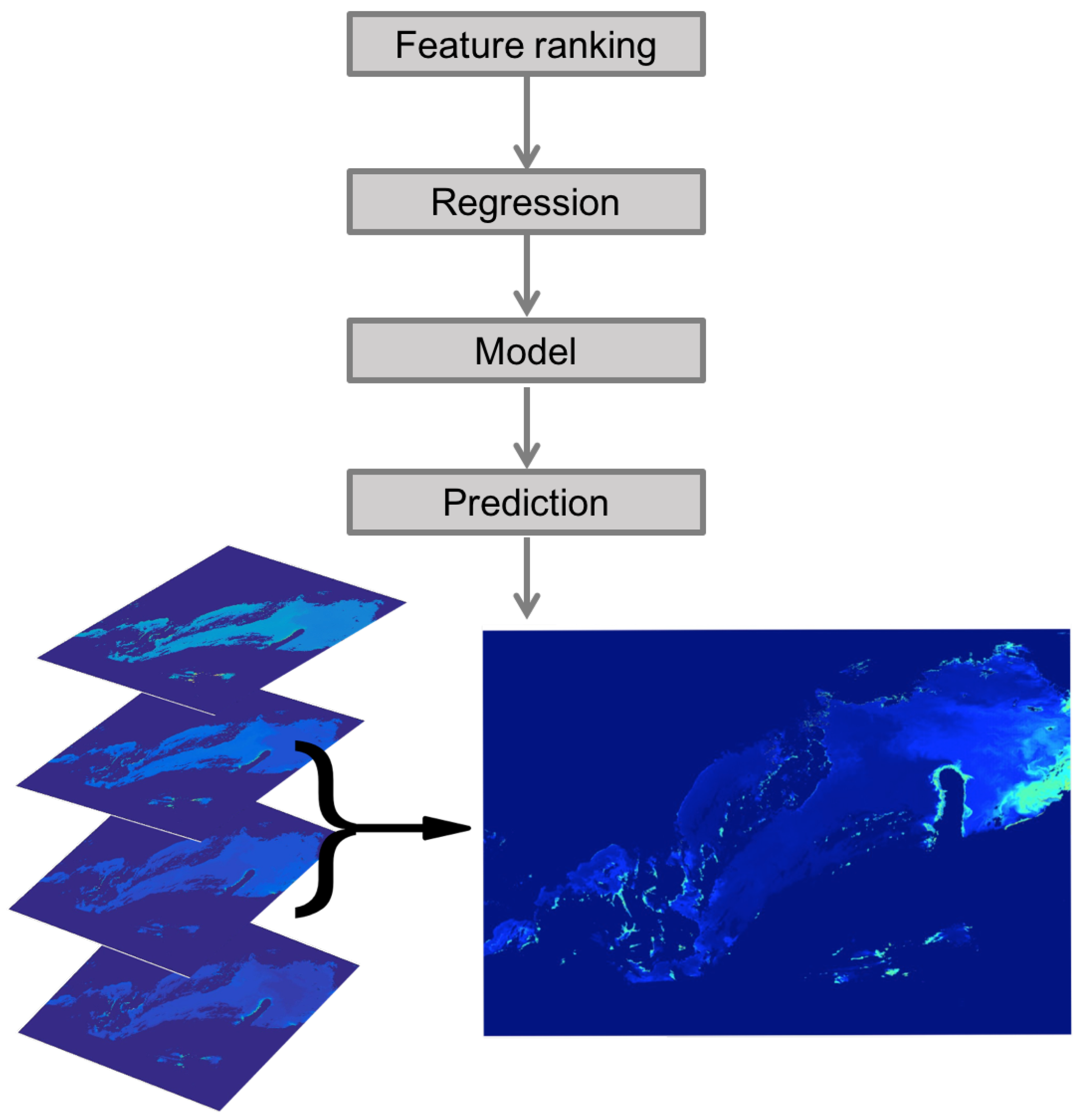
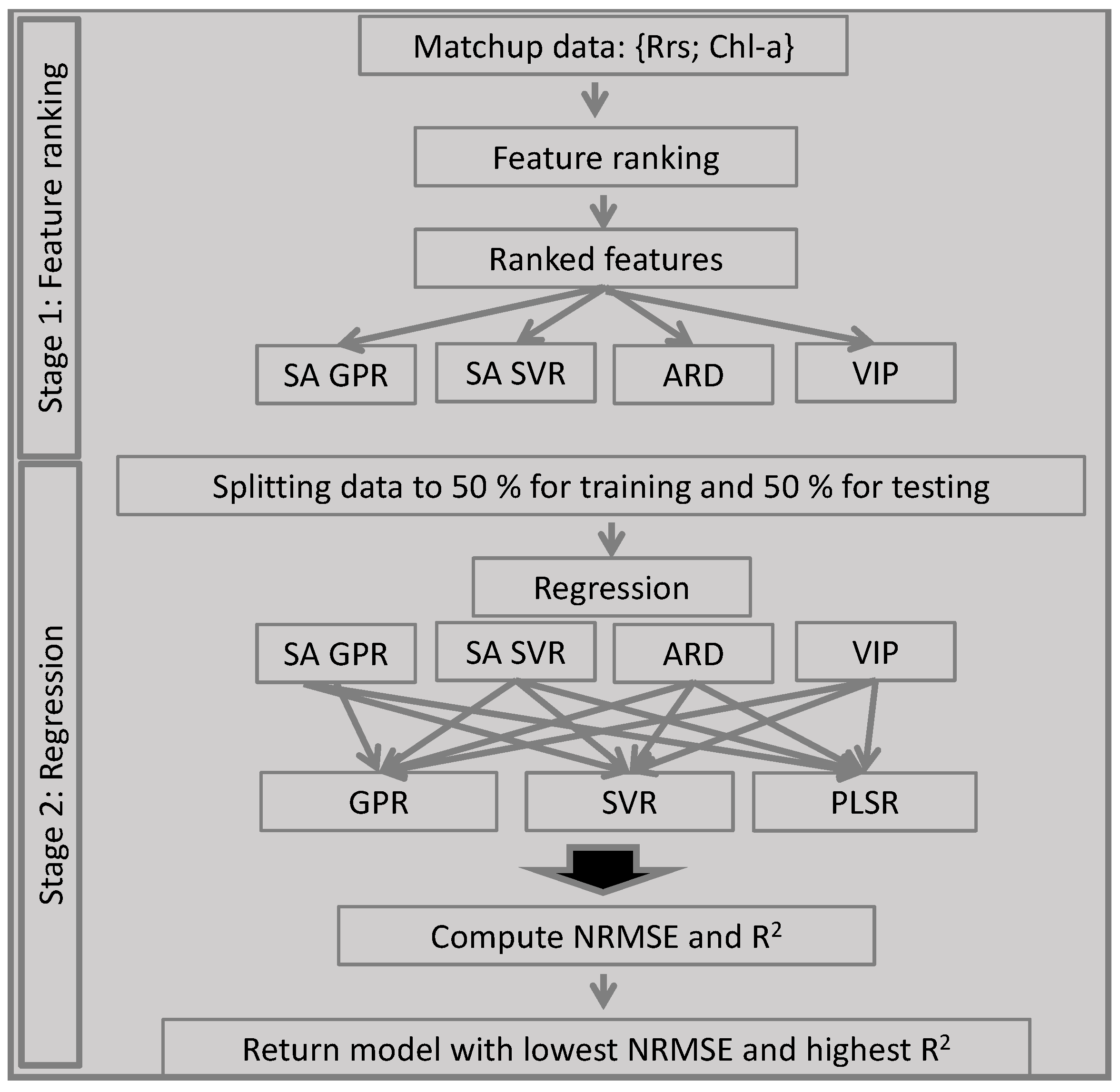
2.2.5. Summary of the AMSA Approach

Figure 4 shows the summary of the ML AMSA for oceanic Chl-a content estimation. The ML AMSA uses in Stage 1 the Chl-a/Rrs matchup dataset to rank the features by using the SA GPR, SA SVR, ARD and VIP feature ranking methods. Then in the Stage 2, the dataset is split to perform regression by the GPR, SVR and PLSR models. Finally, the model with lowest NRMSE and highest R${}^2$ is returned. This is the best model between the available possibilities. Figure 5 shows an illustrative example, how AMSA can be used for applications.

2.3. Data

We evaluated the AMSA algorithm on the IOCCG synthesized dataset [48] and a MERIS (MEdium Resolution Imaging Spectrometer) and MODIS-Aqua (MODerate-resolution Imaging Spectroradiometer) dataset obtained from SeaBASS database [68,69].

Table 2. Summary of the training datasets we used for model selection.

Synthetic resampled MERIS global (MS 1a)
Bands (${\lambda }_c$ (nm))	413 443 490 510 560 620 665 681
Band width	10 nm and 7.5 nm
Spatial resolution	300 m
Chl-a range (mgm${}^{-3}$)	0.03–30
$a_{CDOM}$ (m${}^{-1}$)	0.0025–2.3677
Nr. of samples	478
Synthetic resampled MERIS eutrophic (MS 1b)
Chl-a range (mgm${}^{-3}$)	0.7–30
$a_{CDOM}$ (m${}^{-1}$)	0.06–2.3677
Nr. of samples	300
MERIS global (MS 2a)
Chl-a range (mgm${}^{-3}$)	0.017–40.23
Nr. of samples	557
MERIS eutrophic (MS 2b)
Chl-a range (mgm${}^{-3}$)	0.7076–40.23
Nr. of samples	247
Synthetic resampled MODIS-Aqua global (MS 3a)
Bands (${\lambda }_c$ (nm))	412 443 488 531 551 667 678
Band width	10 nm, 15 nm
Spatial resolution	1000 m
Chl-a range (mgm${}^{-3}$)	0.03–30
$a_{CDOM}$ (m${}^{-1}$)	0.0025–2.3677
Nr. of samples	478
Synthetic resampled MODIS-Aqua eutrophic (MS 3b)
Chl-a range (mgm${}^{-3}$)	0.03–30
$a_{CDOM}$ (m${}^{-1}$)	0.06–2.3677
Nr. of samples	300
MODIS-Aqua global (MS 4a)
Bands (${\lambda }_c$ (nm))	412 443 488 531 551 667 678
Band width	10 nm, 15 nm
Spatial resolution	1000 m
Chl-a range (mgm${}^{-3}$)	0.0153–25.4985
Nr. of samples	579
MODIS-Aqua eutrophic (MS 4b)
Chl-a range (mgm${}^{-3}$)	0.703–25.4985
Nr. of samples	392

summarizes the datasets we used for demonstrating the AMSA algorithm.

2.3.1. Training Data

The synthetic IOCCG dataset has a spectral region ranging from 400 to 800 nm on a 10 nm bandwidth, and containing both inherent (IOPs) and apparent optical properties (AOPs). We resampled the dataset to match the positions and bandwidths of the spectral bands of MERIS and MODIS-Aqua used for OC applications.

The summary of the synthetic resampled dataset can be seen in Table 2. We used the Rrs values with the corresponding Chl-a values. This dataset allows to mimic eutrophic conditions by defining a threshold based on the absorption coefficient for CDOM($a_{CDOM}$) and Chl-a value. We partitioned the resampled data to eutrophic oceanic waters, for $a_{CDOM}>0.06$ m${}^{-1}$ and Chl-a $>0.7$ mgm${}^{-3}$.

The MERIS dataset consists of 567 measurements, measured between April 2002 and March 2012. It can be seen that the Chl-a content spans a wide range of concentration with values in the range between 0.017 and 40.23 mgm${}^{-3}$. The bandwidth is here 10 nm for bands 1–7, and 7.5 nm for band 8.

The MODIS-Aqua dataset has seven channels ranging from 405 nm to 683 nm. The spectral resolution is 10 nm, except for the first band, which has a bandwidth of 15 nm. The data we used here has 579 measurements between July 2002 and November 2012, and the Chl-a concentrations are between 0.0153 and 25.4985 mgm${}^{-3}$.

In case of the MERIS and MODIS-Aqua datasets, only the Rrs and the corresponding Chl-a values were available, thus the division of the data was based on the Chl-a content only. The geographic locations of the measurements can be seen in Figure 6. The red dots indicate measurements for Chl-a value below 0.7 mgm${}^{-3}$, and the black ones for Chl-a above 0.7 mgm${}^{-3}$. It can be seen that measurements corresponding to eutrophic conditions are usually located in the coastal regions.

2.3.2. Test Data

We illustrate the results of the AMSA algorithm for eutrophic conditions on two full resolution images acquired by MERIS (We obtained the Rrs data from https://oceancolor.gsfc.nasa.gov/cgi/browse.pl?sen=am). The chosen areas are assumed to represent optically complex aquatic environments. One of the images is taken over the eastern coast of USA, and the other image is from the southern part of the Baltic sea. For better visualization purposes, we enlarged a part of the image.

3. Results

We applied AMSA to the eight datasets. For each dataset the total combination of models being evaluated by AMSA is (feature ranking) · (number of spectral bands) · (regression models). The total number of model evaluation are 84 and 96 for the MODIS-Aqua (7 bands) and MERIS (8 bands) datasets, respectively. This means that by using feature ranking methods, the total number of model evaluations are reduced, which speeds up the computational time required to return the most optimal model. Feature ranking reduces the total number of possible model-combinations by assigning relevance to the features. After the spectral bands were ranked, the sequential forward selection approach automatically trained and tested all the possible model combinations, and output the best model based on the computed regression performance measures.

Table 3. Selected models for the datasets.

Data Label	Model	Spectral Bands	# of Bands	NRMSE	R${}^2$
MS 1a	GPR by VIP	1,…,7	7	0.0983	0.9463
MS 1b	GPR by VIP	4, 5 and 6	3	0.1363	0.9157
MS 2a	GPR by SA GP	1, 2, 5, 6 and 7	5	0.0764	0.9159
MS 2b	SVR by VIP	4, 5 and 6	3	0.1305	0.8332
MS 3a	GPR by ARD	1, 3 and 7	3	0.1082	0.9353
MS 3b	GPR by ARD	1, 3, 5 and 7	4	0.144	0.9068
MS 4a	SVR by VIP	1, 2, 3, 4, 5 and 7	6	0.1094	0.8402
MS 4b	SVR by ARD	1, 2, 3 and 7	4	0.1180	0.7540

shows the results of the AMSA algorithm for all the datasets. Note that the NMRSE and R${}^2$ values in Table 3 are calculated from the test data.

In case of all the synthetic datasets (MS 1a, MS 1b, MS 3a and MS 3b) the best regression model was found to be the GPR, while for most of the real datasets (MS 2b, MS 4a and MS 4b) the strongest regression was obtained by the SVR model. This can be due to the fact, that the synthetic dataset has low noise level in comparison to the real dataset (The parameter that handles noise in the GPR model, should have been tuned for the real datasets. However, in order to make the AMSA as robust as possible, we chose to compute the initial noise parameter by following the same formula).

For the MERIS datasets the best regression was achieved by using the spectral bands ranked by the VIP ranking method for most of the cases (MS 1a, MS 1b and MS 2b). In case of the MODIS-Aqua datasets, the ARD ranking method seemed to result in the best ranking (MS 3a, MS 3b and MS 4b).

For global monitoring, the best model was obtained by using most of the available spectral bands for almost all cases (MS 1a, MS 2a and MS 4a). The only exception was the synthetic MODIS-Aqua dataset, where the best model was already achieved by using only 3 spectral bands.

For eutrophic conditions AMSA resulted in the best regression, when only three or four bands were used. In case of the MERIS datasets (MS 1b and MS 2b), these bands are centered at 510, 560 and 620 nm. For the MODIS-Aqua datasets bands centered at 412, 488 and 678 nm were included in the regression models for both the synthetic (MS 3b) and real (MS 4b) dataset to achieve the strongest regression model.

The regression performance measures show, that the lowest NRMSE and highest R${}^2$ were achieved for the synthetic global datasets (MS 1a and MS 3a), while the models resulting in highest NRMSE and lowest R${}^2$ were for the eutrophic real datasets (MS 2b and MS 4b). These results also confirm the challenges of Chl-a content estimation from optically complex waters.

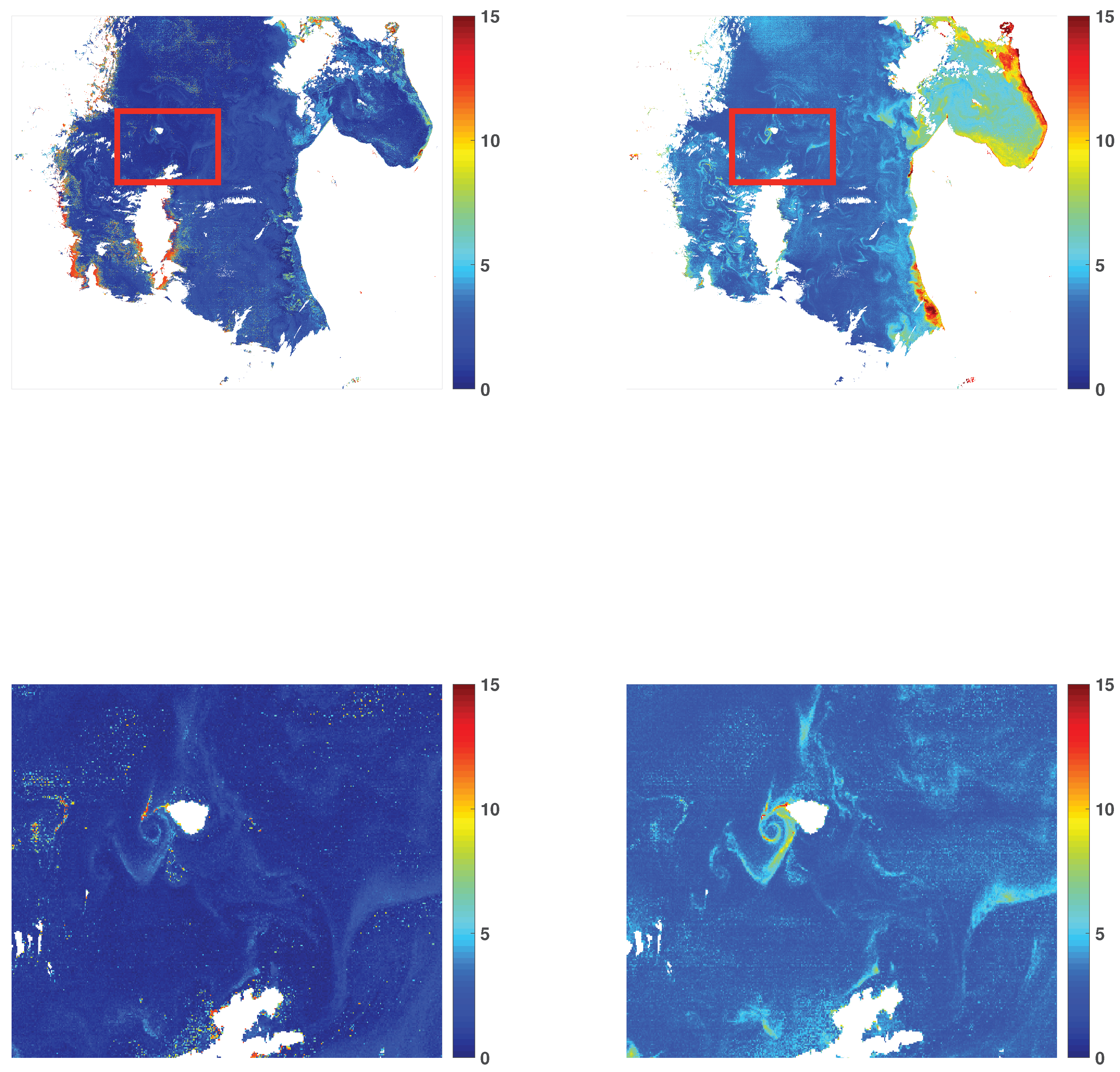
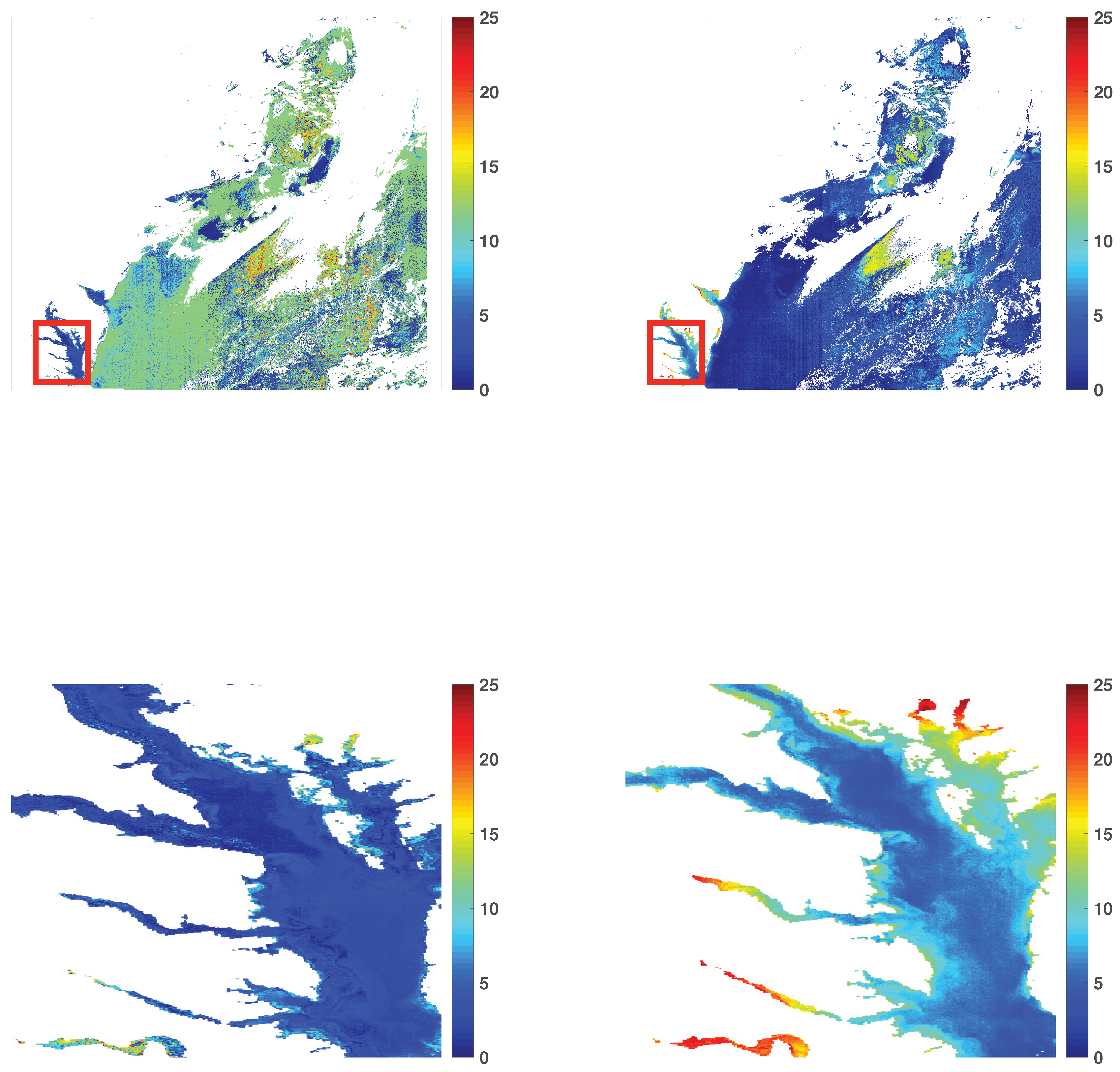
3.1. Chlorophyll-a Maps

In order to illustrate the performance of the best models for eutrophic conditions, we chose two full resolution MERIS images acquired over areas, which are assumed to be optically complex waters.

3.2. Cross Validation

The outputs of AMSA for the MERIS datasets (MS1b and MS2b), were the GPR and SVR models with bands centered at 510, 560 and 620 nm. We used cross validation to assess the robustness of the models. This was done by randomly dividing the datasets (MS1b and MS2b) into 80% for training and 20% for testing. Then training and testing of the models was performed by computing the NRMSE and R${}^2$ measures. This was done in 500 iterations. The mean values of the computed measures for the cross validations can be seen in

Table 4. Results of the cross validation.

MS1b
	NRMSE	R${}^{\mathbf{2}}$
GPR	0.1497	0.8973
SVR	0.1527	0.836
MS2b
	NRMSE	R${}^{\mathbf{2}}$
GPR	0.1464	0.824
SVR	0.1438	0.831

.

The cross validation resulted in very similar computed measures for both models. In case of the MS1b dataset, the GPR model resulted in slightly better values, while for the MS2b data the SVR model showed some improvements. This is in good agreement with the measures output by AMSA (Table 3). The cross validation results also indicate, that in case of the MS1b dataset the difference between the computed regression performance measures for the two models is larger, than is case of the MS2b dataset.

3.3. Visual Illustrations

We applied the AMSA selected GPR and SVR models to the test images. Figure 7 and Figure 8 show the estimated Chl-a content. Figure 7 shows the estimated Chl-a content for the coastal water of East USA by using the GPR (left-column) and SVR (right-column) model with bands centered at 510, 560 and 620 nm. The overall Chl-a maps show that the GPR model predicts higher Chl-a content than the SVR model (top-row). It can be seen in the enlarged area (bottom-row), that there are regions where the SVR model assigns higher values to the Chl-a contents.

Figure 8 shows the estimated Chl-a content maps for the southern part of the Baltic sea. In this case, the overall predicted Chl-a content values (top-row) seem to be more similar for the GPR and SVR models. There are some regional variations in this case as well. The bottom-row in Figure 8 shows the enlarged area. Both models seem to capture the eddies in fine details.

4. Discussion

In this work, we presented a strategy to automatically determine the most suitable model for a given dataset for OC applications. The AMSA approach chooses the best model to estimate any water quality parameter from remotely sensed data. AMSA can determine the most suitable model for any regions and sensors. The input to AMSA is the matchup data, and the output is the best model. AMSA also outputs the number and combination of features needed to obtain the output model, and the regression performance measures for the best model.

We presented the AMSA for oceanic Chl-a content estimation by using ML methods. The AMSA we built here, has four feature ranking methods, the SA GPR, SA SVR, ARD and VIP methods, three regression models, the GPR, SVR and PLSR models, and two regression performance measures, the NRMSE and R${}^2$ to evaluate the regression models. The four feature ranking methods are associated with the three sophisticated regression models, therefore it was a natural choice to include them in the AMSA we chose here.

Both the GPR and SVR models have been shown to be strong regression models for OC applications. They are flexible non-linear kernel methods, using kernel functions in the regression stage. The choice of the kernel function is strongly dependent on the nature of the data. Here we used the most common kernel, the squared exponential kernel function, which has several advantageous properties. It is a universal kernel [62], and infinitely differentiable. This is a very important property with regard to the SA feature ranking methods, which uses the partial derivatives of the mean function in the GPR and SVR models. The squared exponential kernel function also allows to assess feature relevance by using the length-scale parameter in the function. The ARD feature ranking method uses the inverse of the optimized length-scale parameter to assign relevance. Optimization is done numerically through the maximum likelihood function, which in some cases can be trapped in a local minimum. This might result in erroneous ranking. Furthermore, the initialization of the parameters in the kernel function also have an impact on the optimization, and hence on the regression as well. Therefore, developing the robustness of initializing these parameters from the data should be prioritized in future methodological development.

Despite the PLSR model differs from the kernel machines in its underlying fundamental principles, it also provides the possibility to assess feature relevance through the VIP method. In this work, the AMSA has not output the PLSR model as the most suitable algorithm for Chl-a content estimation. However, in many cases (see Table 3) the VIP method seemed to rank the spectral bands such that the strongest regression was achieved by using the kernel machines. Thus, using the VIP method for feature ranking and kernel machines for regression might be a good combination of methods.

In this work we showed how these ML methods can be used to build an AMSA to estimate Chl-a content in different water conditions and for different sensors. The chosen matchup datasets (MERIS, MODIS-Aqua and the synthesized IOCCG dataset) allowed us to simulate water conditions with increased complexity. Note, although the Chl-a threshold we set here to 0.7 mgm${}^{-3}$ might be low for optically complex waters, the observations in the real eutrophic datasets above this value, still seem to originate from coastal environments (Figure 6).

AMSA gave as result that for the synthetic datasets the GPR performed best, but for most of the real dataset the best model was obtained with the SVR model. However, the cross validation results suggest that the SVR model might only have slightly better performance than the GPR model for these datasets.

Generally, for global Chl-a content estimation most of the spectral bands were needed to achieve the best regression with the chosen models. This might be due to the larger variety in the data. This result was in contrast to water conditions of increased complexity, where using only three or four of the available spectral bands as inputs resulted the strongest regression. In case of MERIS, these bands were centered at 510, 560 and 620 nm for both the synthetic and real datasets. The spectral band at 510 nm is used to estimate Chl-a content in CDOM rich waters [70]. This is due to the fact that both CDOM and Chl-a has absorption in the blue region of the visible part of the electromagnetic spectrum. The spectral band at 510 nm is mostly representative for the accessory pigments. However, since these pigments are strongly correlated with Chl-a, this band has been widely used to estimate Chl-a content from optically complex waters [16,17,70]. Furthermore, the green spectral band, centered at 560 nm is commonly used for Chl-a estimation, since there is little or no absorption due to phytoplankton in this region. Therefore, this is an important band to use as a reference wavelength in many Chl-a content retrieval algorithms [70]. Using red bands, included the band centered at 620 nm, to estimate Chl-a content has also been commonly used for optically complex waters due to the second absorption peak of the Chl-a [16].

For the eutrophic MODIS-Aqua datasets, the spectral bands centered at 412, 488 and 678 nm were found to have importance in the estimation of Chl-a for both the synthesized and real datasets. The bands centered at 488 and 678 nm are in good correspondence with the results for the MERIS datasets. The spectral band centered at 412 nm has also been suggested for Chl-a estimation in complex waters due to the deviation in the absorption between CDOM and Chl-a in this spectral region [71].

Since we used a synthetic resampled dataset to present the performance of AMSA, the model outputs differed from the real datasets. Therefore, we chose to illustrate the best models for both the synthetic and real datasets for eutrophic conditions for the MERIS sensor for applications. In case of the coastal part of eastern USA, the GPR assigned in general higher values to the Chl-a content than the SVR model. However, enlarging a region close to shore revealed that the SVR model estimated higher Chl-a than the GPR model. This was also observable for the southern part of the Baltic sea, with less pronounced differences. The illustrative example also showed that both models could capture the same patterns and reveal fine details. Most probably there is a systematic bias occurring in the models. This can be adjusted by tuning the initial parameters in the kernel function, once the model for a given purpose is determined.

5. Conclusions

We conclude, based on this illustrative study, that the AMSA can be a helpful tool for water quality analysis from remote sensing data. It may also be useful in further development of new algorithms. AMSA can be used to objectively compare models with newly introduced algorithms. Furthermore, AMSA might also contribute to improved understanding of the underlying physical processes for various water conditions due to the inclusion of the feature ranking methods.

We have shown that combining ML feature ranking and regression methods in AMSA can reduce computational time and result in improved regression. Furthermore, kernel machines, such as the GPR and SVR models are confirmed to show strong regression power.

For future work, we plan to generalize AMSA by extending the methodology and applying it to different complex aquatic environments and sensors. We also plan to design a flexible AMSA so that user defined models can be added.

References

1. Kahru, M.; Mitchell, B.G. Ocean Color Reveals Increased Blooms in Various Parts of the World. Eos Trans. Am. Geophys. Union 2008, 89, 170. [Google Scholar] [CrossRef]
2. McClain, C.R. A Decade of Satellite Ocean Color Observations. Ann. Rev. Mar. Sci. 2009, 1, 19–42. [Google Scholar] [CrossRef] [PubMed]
3. Gholizadeh, M.H.; Melesse, A.M.; Reddi, L. A Comprehensive Review on Water Quality Parameters Estimation Using Remote Sensing Techniques. Sensors 2016, 16, 1298. [Google Scholar] [CrossRef] [PubMed]
4. Wilson, C. The rocky road from research to operations for satellite ocean-colour data in fishery management. ICES J. Mar. Sci. 2011, 68, 677–686. [Google Scholar] [CrossRef]
5. Ha, N.T.T.; Koike, K.; Nhuan, M.T. Improved Accuracy of Chlorophyll-a Concentration Estimates from MODIS Imagery Using a Two-Band Ratio Algorithm and Geostatistics: As Applied to the Monitoring of Eutrophication Processes over Tien Yen Bay (Northern Vietnam). Remote Sens. 2014, 6, 421–442. [Google Scholar] [CrossRef]
6. Yang, X.E.; Wu, X.; Hao, H.L.; He, Z.L. Mechanisms and assessment of water eutrophication. J. Zhejiang Univ. Sci. B 2008, 9, 197–209. [Google Scholar] [CrossRef] [PubMed]
7. Behrenfeld, M.J.; O’Malley, R.T.; Siegel, D.A.; McClain, C.R.; Sarmiento, J.L.; Feldman, G.C.; Milligan, A.J.; Falkowski, P.G.; Letelier, R.M.; Boss, E.S. Climate-driven trends in contemporary ocean productivity. Nature 2006, 444, 752–755. [Google Scholar] [CrossRef] [PubMed]
8. Ritchie, J.C.; Zimba, P.V.; Everitt, J.H. Remote Sensing Techniques to Assess Water Quality. Photogramm. Eng. Remote Sens. 2003, 69, 695–704. [Google Scholar] [CrossRef]
9. Govindjee. Bioenergetics of Photosynthesis; Academic Press: Cambridge, MA, USA, 1975. [Google Scholar]
10. Volk, T.; Hoffert, M.I. Ocean Carbon Pumps: Analysis of Relative Strengths and Efficiencies in Ocean-Driven Atmospheric CO2 Changes; American Geophysical Union: Washington, DC, USA, 2013; pp. 99–110. [Google Scholar]
11. Arrigo, K.R.; Robinson, D.H.; Worthen, D.L.; Dunbar, R.B.; DiTullio, G.R.; VanWoert, M.; Lizotte, M.P. Phytoplankton Community Structure and the Drawdown of Nutrients and CO2 in the Southern Ocean. Science 1999, 283, 365–367. [Google Scholar] [CrossRef] [PubMed]
12. Hein, M.; Sand-Jensen, K. CO2 increases oceanic primary production. Nature 1997, 388, 526–527. [Google Scholar] [CrossRef]
13. Hofmann, M.; Worm, B.; Rahmstorf, S.; Schellnhuber, H.J. Declining ocean chlorophyll under unabated anthropogenic CO2 emissions. Environ. Res. Lett. 2011, 6, 34–35. [Google Scholar] [CrossRef]
14. Hu, C.; Lee, Z.; Franz, B. Chlorophyll a algoritms for oligotrophic oceans: A novel approach based on three-band reflectance difference. J. Geophys. Res. 2012, 117. [Google Scholar] [CrossRef]
15. Morel, A.; Maritorena, S. Bio-optical properties of oceanic waters: A reappraisal. J. Geophys. Res. Ocean. 2001, 106, 7163–7180. [Google Scholar] [CrossRef]
16. O’Reilly, J.E.; Maritirena, S.; Mitchell, B.G.; Siegel, D.A.; Carder, K.L.; Garver, S.A.; Kahru, M.; McClain, C. Ocean color chlorophyll algorithms for SeaWiFS. J. Geophys. Res. 1998, 103, 24937–24953. [Google Scholar] [CrossRef]
17. O’Reilly, J.E.; Maritorena, S.; O’Brien, M.C.; Siegel, D.A.; Toole, D.; Menzies, D.; Smith, R.C.; Mueller, J.L.; Mitchell, B.G.; Kahru, M.; et al. SeaWiFS Postlaunch Calibration and Validation Analyses, Part 3. Nasa Tech. Memo. 2000, 11, 3–8. [Google Scholar]
18. Werdell, P.J.; Bailey, S.W. An improved bio-optical data set for ocean color algorithm development and satellite data product validation. Remote Sens. Environ. 2005, 98, 122–140. [Google Scholar] [CrossRef]
19. Blondeau-Patissier, D.; Gower, J.F.; Dekker, A.G.; Phinn, S.R.; Brando, V.E. A review of ocean color remote sensing methods and statistical techniques for the detection, mapping and analysis of phytoplankton blooms in coastal and open oceans. Prog. Oceanogr. 2014, 123, 123–144. [Google Scholar] [CrossRef] [Green Version]
20. Matthews, M.W. A current review of empirical procedures of remote sensing in inland and near-coastal transitional waters. Int. J. Remote Sens. 2011, 32, 6855–6899. [Google Scholar] [CrossRef]
21. Odermatt, D.; Gitelson, A.; Brando, V.E.; Schaepman, M. Review of constituent retrieval in optically deep and complex waters from satellite imagery. Remote Sens. Environ. 2012, 118, 116–126. [Google Scholar] [CrossRef] [Green Version]
22. Gitelson, A.A.; Schalles, J.F.; Hladik, C.M. Remote chlorophyll-a retrieval in turbid, productive estuaries: Chesapeake Bay case study. Remote Sens. Environ. 2007, 109, 464–472. [Google Scholar] [CrossRef]
23. Wang, T.S.; Tan, C.H.; Chen, L.; Tsai, Y.C. Applying Artificial Neural Networks and Remote Sensing to Estimate Chlorophyll-a Concentration in Water Body. Int. Symp. Intell. Inf. Technol. Appl. 2008, 1, 540–544. [Google Scholar]
24. Canziani, G.; Ferrati, R.; Marinelli, C.; Dukatz, F. Artificial neural networks and remote sensing in the analysis of the highly variable Pampean shallow lakes. Math. Biosci. Eng. 2008, 5, 691–711. [Google Scholar] [CrossRef] [PubMed]
25. Gross, L.; Thiria, S.; Frouin, R. Applying artificial neural network methodology to ocean color remote sensing. Ecol. Modell. 1999, 120, 237–246. [Google Scholar] [CrossRef]
26. Nabavi-Pelesaraei, A.; Bayat, R.; Hosseinzadeh-Bandbafha, H.; Afrasyabi, H.; Chau, K.-W. Modeling of energy consumption and environmental life cycle assessment for incineration and landfill systems of municipal solid waste management—A case study in Tehran Metropolis of Iran. J. Clean. Prod. 2017, 148, 427–440. [Google Scholar] [CrossRef]
27. Chen, X.Y.; Chau, K.W. A Hybrid Double Feedforward Neural Network for Suspended Sediment Load Estimation. Water Resour. Manag. 2016, 30, 2179–2194. [Google Scholar] [CrossRef]
28. Alizadeh, M.J.; Kavianpour, M.R.; Kisi, O.; Nourani, V. A new approach for simulating and forecasting the rainfall-runoff process within the next two months. J. Hydrol. 2017, 548, 588–597. [Google Scholar] [CrossRef]
29. Zhan, H.; Shi, P.; Chen, C. Retrieval of Oceanic Chlorophyll Concentration Using Support Vector Machines. IEEE Trans. Geosci. Remote Sens. 2003, 41, 2947–2951. [Google Scholar] [CrossRef]
30. Camps-Valls, G.; Gómez-Chova, L.; Muñoz-Marí, J.; Vila-Francés, J.; Amorós-López, J.; Calpe-Maravilla, J. Retrieval of oceanic chlorophyll concentration with relevance vector machines. Remote Sens. Environ. 2006, 105, 23–33. [Google Scholar] [CrossRef]
31. Blix, K.; Camps-Valls, G.; Jenssen, R. Gaussian Process Sensitivity Analysis for Oceanic Chlorophyll Estimation. IEEE J. Sel. Top. Appl. Earth Obs. Remote Sens. 2017, 10, 1265–1277. [Google Scholar] [CrossRef]
32. Blix, K.; Eltoft, T. Evaluation of Feature Ranking and Regression Methods for Oceanic Chlorophyll-a Estimation. IEEE J. Sel. Top. Appl. Earth Obs. Remote Sens. 2018, 11, 1403–1418. [Google Scholar] [CrossRef]
33. Sawaya, K.E.; Olmanson, L.G.; Heinert, N.J.; Brezonik, P.L.; Bauer, M.E. Extending satellite remote sensing to local scales: Land and water resource monitoring using high-resolution imagery. Remote Sens. Environ. 2003, 88, 144–156. [Google Scholar] [CrossRef]
34. Brando, V.E.; Dekker, A.G. Satellite hyperspectral remote sensing for estimating estuarine and coastal water quality. IEEE Trans. Geosci. Remote Sens. 2003, 41, 1378–1387. [Google Scholar] [CrossRef]
35. Vargas, M.; Brown, C.W.; Sapiano, M.R.P. Phenology of marine phytoplankton from satellite ocean color measurements. Geophys. Res. Lett. 2009, 36. [Google Scholar] [CrossRef]
36. D’Alimonte, D.; Melin, F.; Zibordi, G.; Berthon, J.F. Use of the novelty detection technique to identify the range of applicability of empirical ocean color algorithms. IEEE Trans. Geosci. Remote Sens. 2003, 41, 2833–2843. [Google Scholar] [CrossRef]
37. Fukushima, H.; Higurashi, A.; Mitomi, Y.; Nakajima, T.; Noguchi, T.; Tanaka, T.; Toratani, M. Correction of atmospheric effect on ADEOS/OCTS ocean color data: Algorithm description and evaluation of its performance. J. Oceanogr. 1998, 54, 417–430. [Google Scholar] [CrossRef]
38. Guyon, I.; Elisseeff, A. An Introduction to Feature Extraction. In Feature Extraction: Foundations and Applications; Springer: Berlin/Heidelberg, Germany, 2006; pp. 1–25. [Google Scholar]
39. Ferreira, E. Model Selection in Time Series Machine Learning Applications. Ph.D. Thesis, University of Oulu, Oulu, Finland, 2015. [Google Scholar]
40. Verrelst, J.; Alonso, L.; Camps-Valls, G.; Delegido, J.; Moreno, J. Retrieval of Vegetation Biophysical Parameters Using Gaussian Process Techniques. IEEE Trans. Geosci. Remote Sens. 2012, 50, 1832–1843. [Google Scholar] [CrossRef]
41. Verrelst, J.; Muñoz, J.; Alonso, L.; Rivera, J.P.; Camps-Valls, G.; Moreno, J. Machine learning regression algorithms for biophysical parameter retrieval: Opportunities for Sentinel-2 and -3. Remote Sens. Environ. 2012, 118, 127–139. [Google Scholar] [CrossRef]
42. Verrelst, J.; Rivera, J.P.; Gitelson, A.; Delegido, J.; Moreno, J.; Camps-Valls, G. Spectral band selection for vegetation properties retrieval using Gaussian processes regression. Int. J. Appl. Earth Obs. Geoinf. 2016, 52, 554–567. [Google Scholar] [CrossRef]
43. Kwiatkowska, E.J.; Fargion, G.S. Application of Machine-Learning Techniques Toward the Creation of a Consistent and Calibrated Global Chlorophyll Concentration Baseline Dataset Using Remotely Sensed Ocean Color Data. IEEE Trans. Geosci. Remote Sens. 2003, 41, 2844–2860. [Google Scholar] [CrossRef]
44. Camps-Valls, G.; Muñoz-Marí, J.; Gómez-Chova, L.; Richter, K.; Calpe-Maravilla, J. Biophysical Parameter Estimation With a Semisupervised Support Vector Machine. IEEE Geosci. Remote Sens. Lett. 2009, 6, 248–252. [Google Scholar] [CrossRef]
45. Rasmussen, P.M.; Madsen, K.H.; Lund, T.E.; Hansen, L.K. Visualization of nonlinear kernel models in neuroimaging by sensitivity maps. NeuroImage 2011, 55, 1120–1131. [Google Scholar] [CrossRef] [PubMed]
46. Wold, S.; Sjöström, M.; Eriksson, L. PLS-regression: a basic tool of chemometrics. Chem. Intell. Lab. Syst. 2001, 58, 109–130. [Google Scholar] [CrossRef]
47. Ryan, K.; Ali, K. Application of a partial least-squares regression model to retrieve chlorophyll-a concentrations in coastal waters using hyper-spectral data. Ocean Sci. J. 2016, 51, 209–221. [Google Scholar] [CrossRef]
48. Lee, Z.P. Remote Sensing of Inherent Optical Properties: Fundamentals, Test of Algorithms, and Applications; Technical Report; International Ocean-Colour Coordinating Group, IOCCG: Busan, Korea, 2006. [Google Scholar]
49. Rasmussen, C.E.; Williams, C.K.I. Gaussian Process for Machine Learning; MIT Press: Cambridge, MA, USA, 2006. [Google Scholar]
50. Smola, A.J.; Schölkopf, B. A tutorial on support vector regression. Stat. Comput. 2004, 14, 199–222. [Google Scholar] [CrossRef]
51. Schölkopf, B.; Smola, A. Learning with Kernels-Support Vector Machines, Regularization, Optimization and Beyond; MIT Press: Cambridge, MA, USA, 2002. [Google Scholar]
52. Murphy, K.P. Machine Learning A probabilistic Perspective; MIT Press: Cambridge, MA, USA, 2012; pp. 496–498. [Google Scholar]
53. Kung, S.Y. Kernel Methods and Machine Learning; Cambridge University Press: Cambridge, UK, 2014; pp. 381–383. [Google Scholar]
54. Gosselin, R.; Rodrigue, D.; Duchesne, C. A Bootstrap-VIP approach for selecting wavelength intervals in spectral imaging applications. Chem. Intell. Lab. Syst. 2010, 100, 12–21. [Google Scholar] [CrossRef]
55. Afanador, N.L. Important Variable Selection in Partial Least Squares for Industrial Process Understanding and Control. Ph.D. Thesis, Radboud University Nijmegen, Nijmegen, The Netherlands, 2014. [Google Scholar]
56. Abdi, H. Partial least squares regression and projection on latent structure regression (PLS Regression). Wiley Int. Rev. Comput. Stat. 2010, 2, 97–106. [Google Scholar] [CrossRef]
57. Rännar, S.; Lindgren, F.; Geladi, P.; Wold, S. A PLS kernel algorithm for data sets with many variables and fewer objects. Part 1: Theory and algorithm. J. Chem. 1994, 8, 111–125. [Google Scholar] [CrossRef]
58. De Jong, S. SIMPLS: An alternative approach to partial least squares regression. Chem. Intell. Lab. Syst. 1993, 18, 251–263. [Google Scholar] [CrossRef]
59. Dayal, B.S.; MacGregor, J.F. Improved PLS algorithms. J. Chem. 1997, 11, 73–85. [Google Scholar] [CrossRef]
60. Song, K.; Lu, D.; Li, L.; Li, S.; Wang, Z.; Du, J. Remote sensing of chlorophyll-a concentration for drinking water source using genetic algorithms (GA)-partial least square (PLS) modeling. Ecol. Inf. 2012, 10, 25–36. [Google Scholar] [CrossRef]
61. Blix, K.; Camps-Valls, G.; Jenssen, R. Sensitivity Analysis of Gaussian Processes for Oceanic Chlorophyll Prediction. In Proceedings of the IEEE International Geoscience and Remote Sensing Symposium, IGARSS, Milan, Italy, 26–31 July 2015; pp. 996–999. [Google Scholar]
62. Micchelli, C.A.; Xu, Y.; Zhang, H. Universal Kernels. J. Mach. Learn. Res. 2006, 7, 2651–2667. [Google Scholar]
63. Eriksson, L.; Johansson, E.; Kettaneh-Wold, N.; Wold, S. Multi- and Megavariate Data Analysis. Principles and Applications. J. Chem. 2001, 16, 261–262. [Google Scholar]
64. Jonsson, P. Surface Status Classification, Utilizing Image Sensor Technology and Computer Models. Ph.D. Thesis, Mid Sweden University, Sundsvall, Sweden, 2015. [Google Scholar]
65. Mehmood, T.; Liland, K.H.; Snipen, L.; Sæbø, S. A review of variable selection methods on Partial Least Squares Regression. Chem. Intell. Lab. Syst. 2012, 118, 62–69. [Google Scholar] [CrossRef]
66. Liang, L.; Qin, Z.; Zhao, S.; Di, L.; Zhang, C.; Deng, M.; Lin, H.; Zhang, L.; Wang, L.; Liu, Z. Estimating crop chlorophyll content with hyperspectral vegetation indices and the hybrid inversion method. Int. J. Remote Sens. 2016, 37, 2923–2949. [Google Scholar] [CrossRef]
67. Sayuri, F.; Watanabe, F.; Alcantara, E.; Walesza, T.; Rodrigues, T.; Imai, N.; Clemente, C.; Barbosa, C.; Luiz, H.; Da, S.; et al. Estimation of Chlorophyll-a Concentration and the Trophic State of the Barra Bonita Hydroelectric Reservoir Using OLI/Landsat-8 Images. Int. J. Environ. Res. Public Health 2015, 12, 10391–10417. [Google Scholar]
68. Werdell, P.J.; Bailey, S.W. The SeaWIFS Bio-optical Archive and Storage System (SeaBASS): Current architeture and implementation. In NASA Technical Memoranda 2002-211617; Fargion, G.S., McClain, C.R., Eds.; NASA Goddard Space Flight Center: Greenbelt, MD, USA, 2002; p. 45. [Google Scholar]
69. Werdell, P.J.; Bailey, S.W.; Fargion, G.S.; Pietras, C.; Knobelspiesse, K.D.; Feldman, G.C.; McClain, C.R. Unique data repository facilitates ocean color satellite validation. EOS Trans. AGU 2003, 84, 387. [Google Scholar] [CrossRef]
70. Cannizzaro, J.P.; Carder, K.L. Estimating chlorophyll a concentrations from remote-sensing reflectance in optically shallow waters. Remote Sens. Environ. 2006, 101, 13–24. [Google Scholar] [CrossRef]
71. Wei, J.; Lee, Z. Retrieval of phytoplankton and colored detrital matter absorption coefficients with remote sensing reflectance in an ultraviolet band. Appl. Opt. 2015, 54, 636–649. [Google Scholar] [CrossRef] [PubMed]
Figure 1. The feature ranking stage of the AMSA.
Remotesensing 10 00775 g001
Figure 2. Regression stage of the AMSA (A).
Remotesensing 10 00775 g002
Figure 3. Regression stage of the AMSA (B).
Remotesensing 10 00775 g003
Figure 4. The ML AMSA for oceanic Chl-a content estiamtion.
Remotesensing 10 00775 g004
Figure 5. Illustration of the AMSA for application.
Remotesensing 10 00775 g005
Figure 6. Position of the data for the MERIS (left) and MODIS-Aqua (right) global dataset. The red and black markers indicate oligotrophic and eutrophic conditions, respectively.
Remotesensing 10 00775 g006
Figure 7. Estimated Chl-a map for the coast of East USA by using the GPR (left-column) and SVR (right-column) model with bands centered at 510, 560 and 620 nm. The bottom row shows the enlarged area indicated by the red squares.
Remotesensing 10 00775 g007
Figure 8. Estimated Chl-a map for the southern Baltic sea by using the GPR (left-column) and SVR (right-column) model with bands centered at 510, 560 and 620 nm. The bottom row shows the enlarged area indicated by the red squares.
Remotesensing 10 00775 g008