A Modified Spatiotemporal Fusion Algorithm Using Phenological Information for Predicting Reflectance of Paddy Rice in Southern China

Abstract
:
1. Introduction
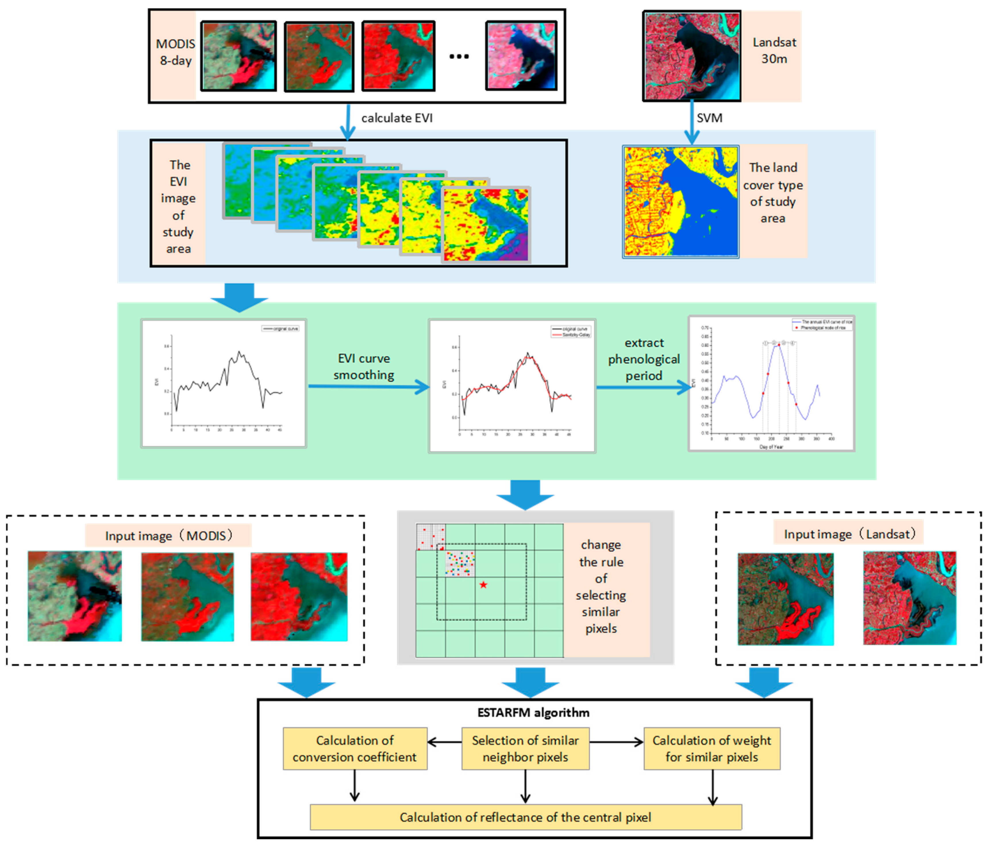
2. Proposed Methodology
2.1. Essential Theories of ESTARFM
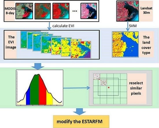
2.2. The Modified Spatiotemporal Algorithm Using Phenological Information for Predicting the Reflectance of Paddy Rice
2.2.1. Construction of the EVI Time Series of Coarse-Resolution Images
2.2.2. Extraction of Paddy Rice Phenology Period from EVI Time Series
2.2.3. Creation of a New Rule of Searching for Similar Neighborhood Pixels
2.2.4. Calculation of the Prediction Reflectance
3. Materials
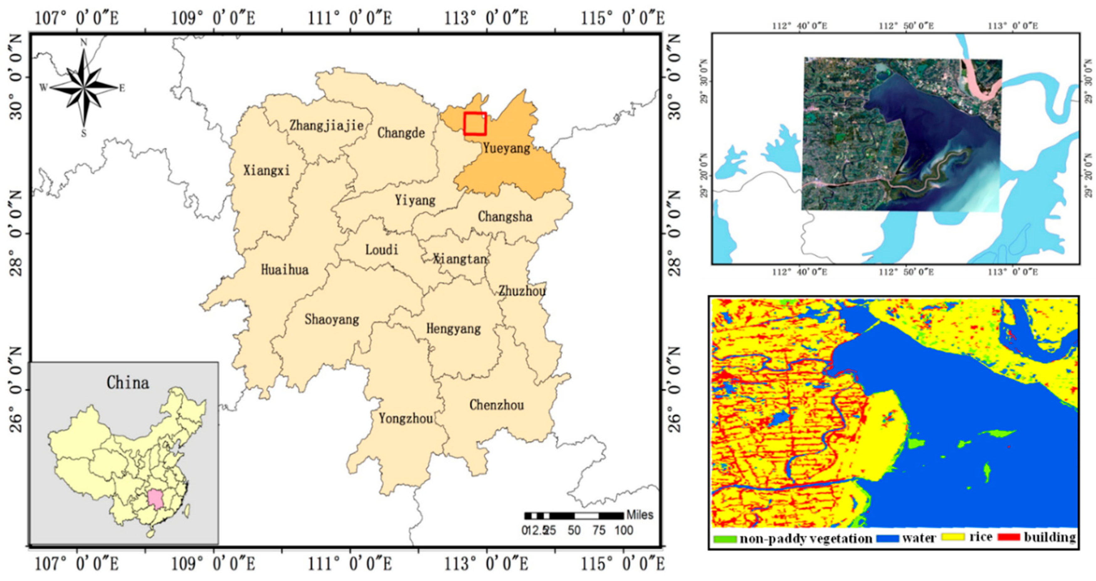
3.1. Study Area
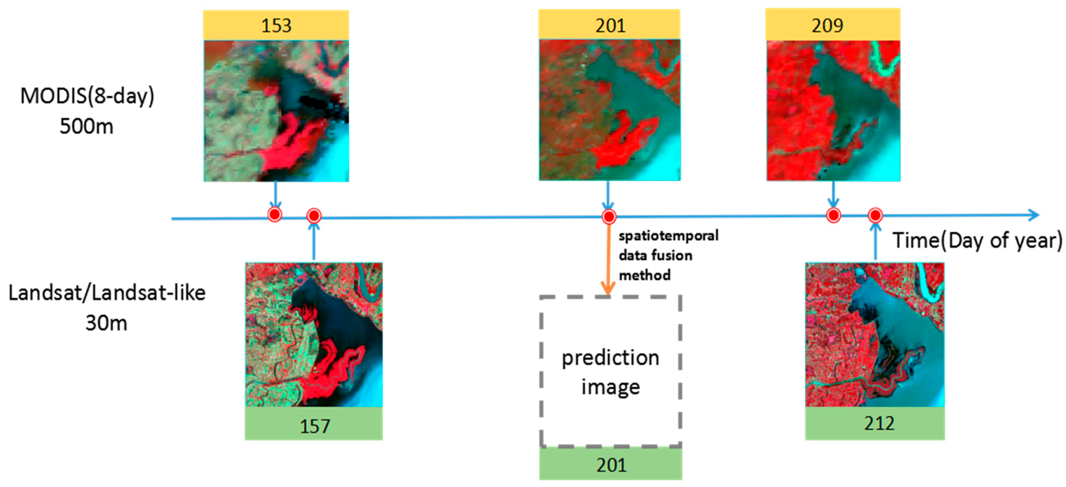
3.2. Satellite Data and Preprocessing
3.3. Algorithm Implementation
4. Results
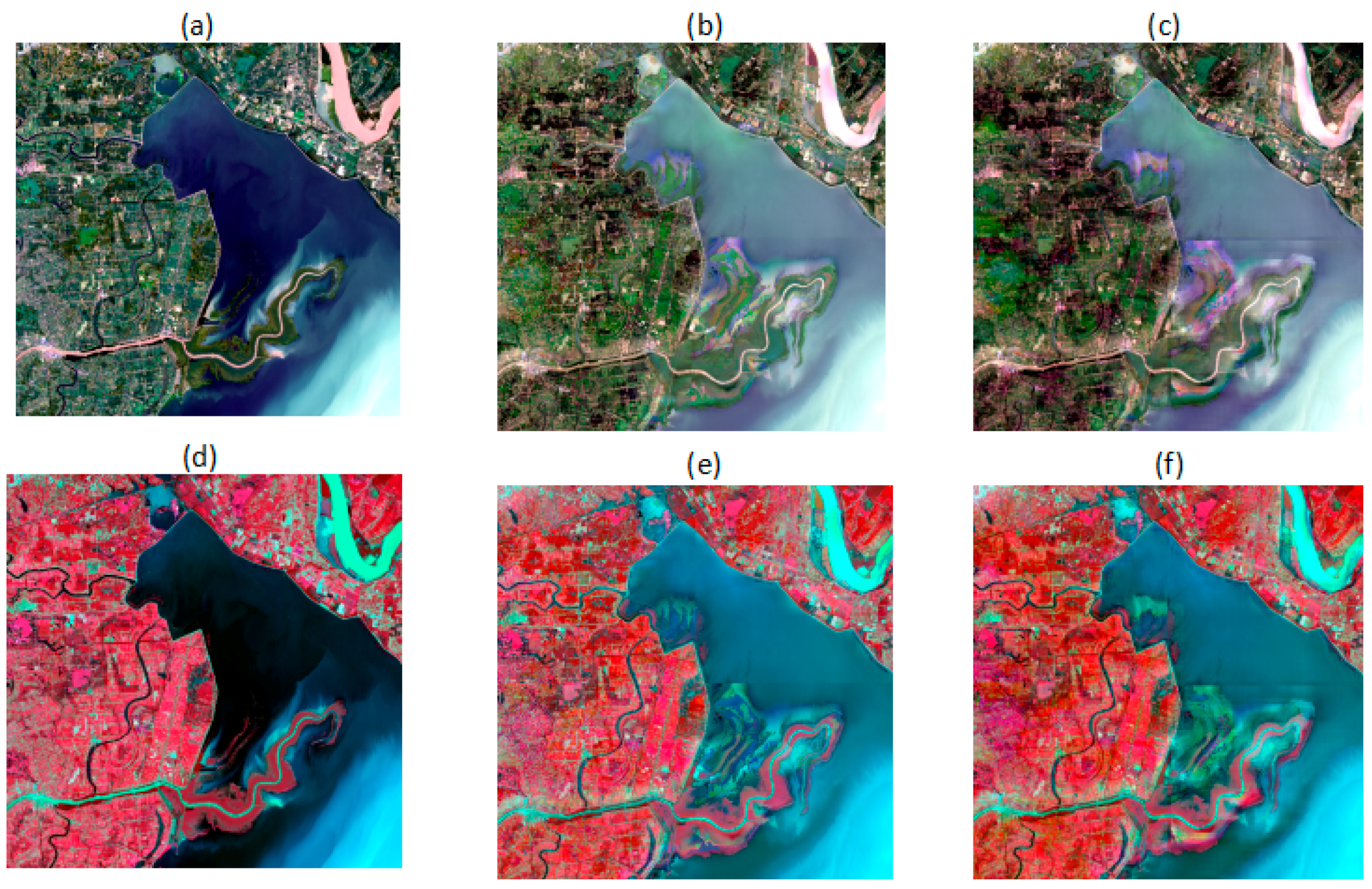
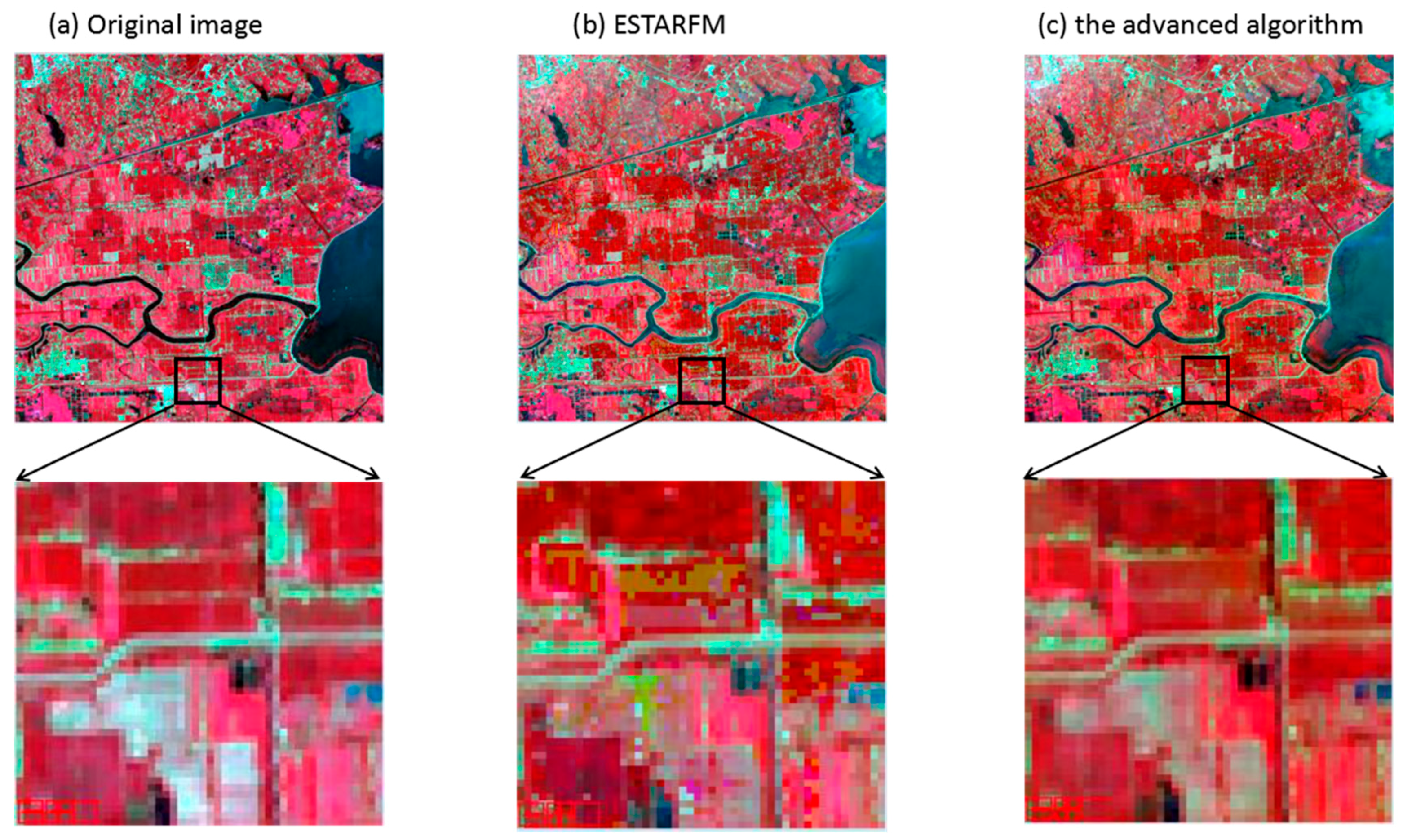
4.1. Comparison with an Actual Image in Visual Details
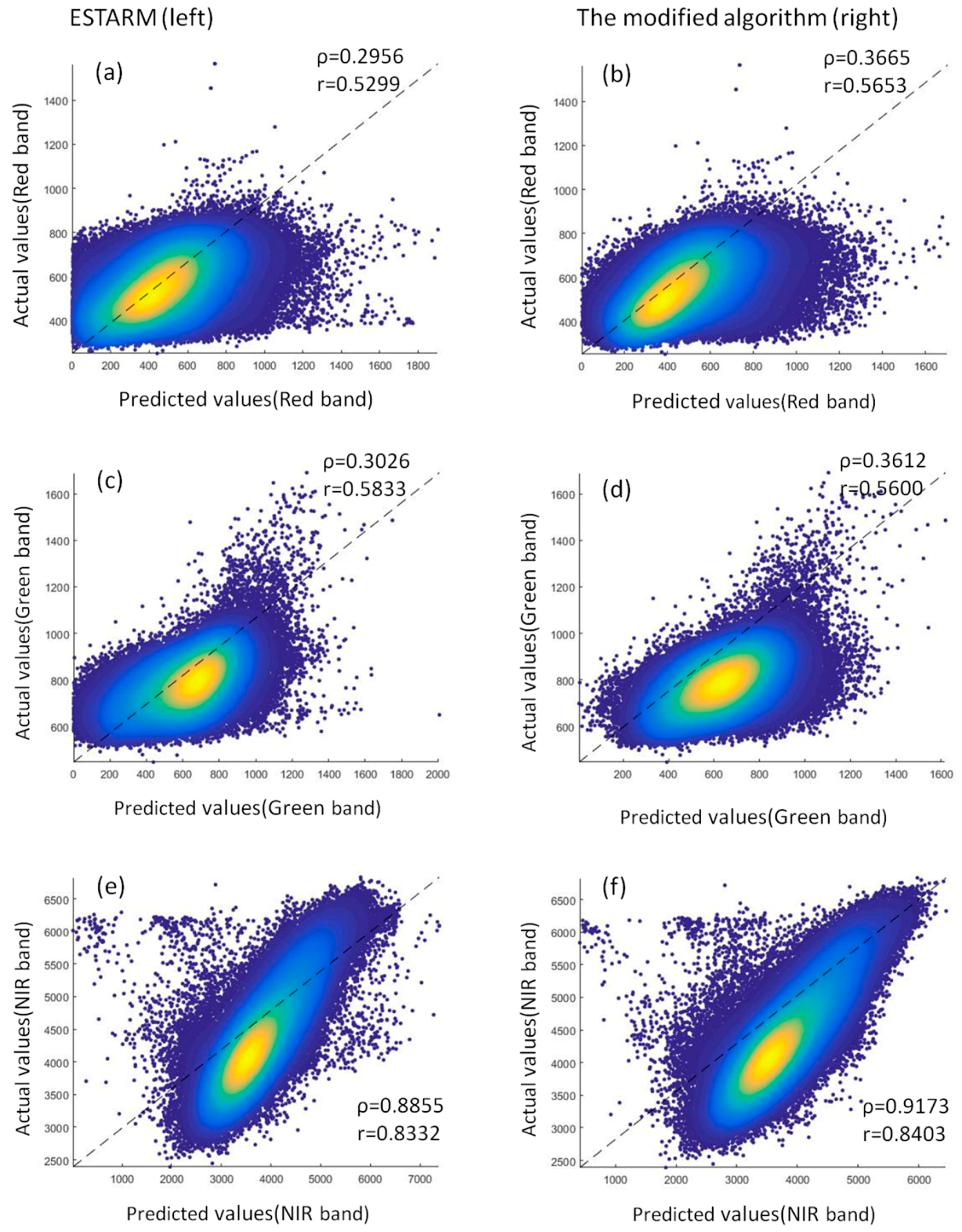
4.2. Comparison with an Actual Image in Reflectance of Paddy Rice
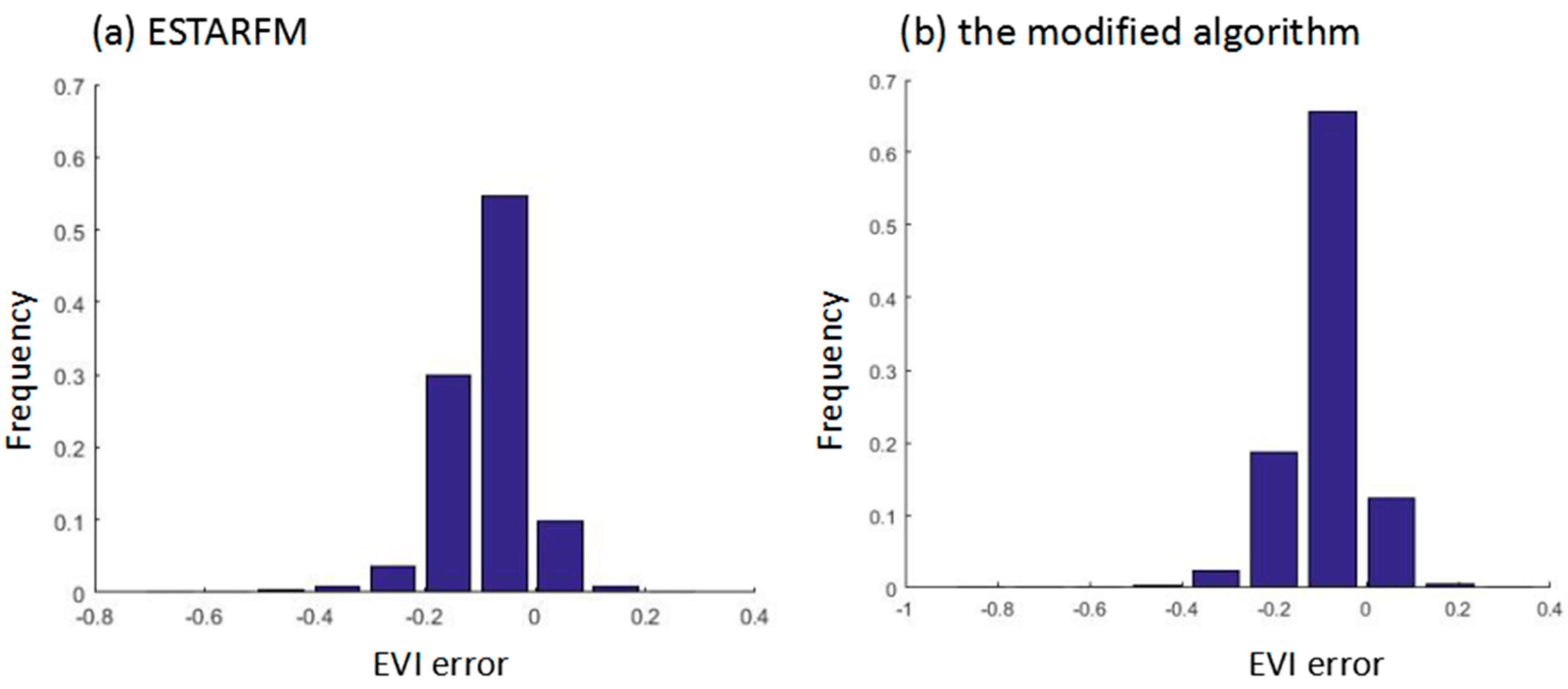
4.3. Comparison with an Actual Image in EVI of Paddy Rice
4.4. Robustness Test of the Modified Algorithm
5. Discussions
6. Conclusions
Author Contributions
Funding
Acknowledgements
Conflicts of Interest
References
- Vogelman, J.E.; Howard, S.M.; Yang, L.M.; Larson, C.R.; Wylie, B.K.; Driel, N.V. Completion of the 1990s national land cover data set for the conterminous united states from landsat thematic mapper data and ancillary data sources. Photogramm. Eng. Remote Sens. 2001, 67, 650–662. [Google Scholar]
- Hansen, M.C.; Roy, D.P.; Lindquist, E.; Adusei, B.; Justice, C.O.; Altstatt, A. A method for integrating modis and landsat data for systematic monitoring of forest cover and change in the congo basin. Remote Sens. Environ. 2008, 112, 2495–2513. [Google Scholar] [CrossRef]
- Cai, S.; Liu, D.; Sulla-Menashe, D.; Friedl, M.A. Enhancing modis land cover product with a spatial–temporal modeling algorithm. Remote Sens. Environ. 2014, 147, 243–255. [Google Scholar] [CrossRef]
- Zhu, X.L.; Jin, C.; Feng, G.; Chen, X.H.; Masek, J.G. An enhanced spatial and temporal adaptive reflectance fusion model for complex heterogeneous regions. Remote Sens. Environ. 2010, 114, 2610–2623. [Google Scholar] [CrossRef]
- Wang, Q.; Atkinson, P.M. Spatio-temporal fusion for daily sentinel-2 images. Remote Sens. Environ. 2017, 204, 31–42. [Google Scholar] [CrossRef]
- Ghassemian, H. A review of remote sensing image fusion methods. Inf. Fusion 2016, 32, 75–89. [Google Scholar] [CrossRef]
- Wei, J.; Wang, L.; Liu, P.; Chen, X.; Li, W.; Zomaya, A.Y. Spatiotemporal fusion of modis and landsat-7 reflectance images via compressed sensing. IEEE Trans. Geosci. Remote Sens. 2017, 55, 7126–7139. [Google Scholar] [CrossRef]
- Wu, M.; Wu, C.; Huang, W.; Niu, Z.; Wang, C.; Li, W.; Hao, P. An improved high spatial and temporal data fusion approach for combining landsat and modis data to generate daily synthetic landsat imagery. Inf. Fusion 2016, 31, 14–25. [Google Scholar] [CrossRef]
- Cohen, W.B.; Goward, S.N. Landsat’s role in ecological applications of remote sensing. Bioscience 2004, 54, 535–545. [Google Scholar] [CrossRef]
- Roy, D.P.; Ju, J.; Lewis, P.; Schaaf, C.; Gao, F.; Hansen, M.; Lindquist, E. Multi-temporal modis–landsat data fusion for relative radiometric normalization, gap filling, and prediction of landsat data. Remote Sens. Environ. Interdiscip. J. 2008, 112, 3112–3130. [Google Scholar] [CrossRef]
- Gao, F.; Masek, J.; Schwaller, M.; Hall, F. On the blending of the landsat and modis surface reflectance: Predicting daily landsat surface reflectance. IEEE Trans. Geosci. Remote Sens. 2006, 44, 2207–2218. [Google Scholar]
- Xiao, X.; Boles, S.; Liu, J.; Zhuang, D.; Frolking, S.; Li, C.; Salas, W.; Iii, B.M. Mapping paddy rice agriculture in southern china using multi-temporal modis images. Remote Sens. Environ. 2005, 95, 480–492. [Google Scholar] [CrossRef]
- Hilker, T.; Wulder, M.A.; Coops, N.C.; Seitz, N.; White, J.C.; Feng, G.; Masek, J.G.; Stenhouse, G. Generation of dense time series synthetic landsat data through data blending with modis using a spatial and temporal adaptive reflectance fusion model. Remote Sens. Environ. 2009, 113, 1988–1999. [Google Scholar] [CrossRef]
- Emelyanova, I.V.; Mcvicar, T.R.; Niel, T.G.V.; Li, L.T.; Dijk, A.I.J.M.V. Assessing the accuracy of blending landsat–modis surface reflectances in two landscapes with contrasting spatial and temporal dynamics: A framework for algorithm selection. Remote Sens. Environ. 2013, 133, 193–209. [Google Scholar] [CrossRef]
- Hilker, T.; Wulder, M.A.; Coops, N.C.; Linke, J.; Mcdermid, G.; Masek, J.G.; Gao, F.; White, J.C. A new data fusion model for high spatial- and temporal-resolution mapping of forest disturbance based on landsat and modis. Remote Sens. Environ. 2009, 113, 1613–1627. [Google Scholar] [CrossRef]
- Zhu, X.; Helmer, E.H.; Gao, F.; Liu, D.; Chen, J.; Lefsky, M.A. A flexible spatiotemporal method for fusing satellite images with different resolutions. Remote Sens. Environ. 2016, 172, 165–177. [Google Scholar] [CrossRef]
- Huang, B.; Song, H. Spatiotemporal reflectance fusion via sparse representation. IEEE Trans. Geosci. Remote Sens. 2012, 50, 3707–3716. [Google Scholar] [CrossRef]
- Huang, B.; Zhang, H. Spatio-temporal reflectance fusion via unmixing: Accounting for both phenological and land-cover changes. Int. J. Remote Sens. 2014, 35, 6213–6233. [Google Scholar] [CrossRef]
- Walker, J.J.; Beurs, K.M.D.; Wynne, R.H.; Gao, F. Evaluation of landsat and modis data fusion products for analysis of dryland forest phenology. Remote Sens. Environ. 2012, 117, 381–393. [Google Scholar] [CrossRef]
- Pan, Y.; Le, L.I.; Zhang, J.; Liang, S. Crop area estimation based on modis-evi time series according to distinct characteristics of key phenology phases:A case study of winter wheat area estimation in small-scale area. J. Remote Sens. 2011, 15, 578–594. [Google Scholar]
- Zhang, X.; Friedl, M.A.; Schaaf, C.B.; Strahler, A.H.; Hodges, J.C.F.; Gao, F.; Reed, B.C.; Huete, A. Monitoring vegetation phenology using modis. Remote Sens. Environ. 2003, 84, 471–475. [Google Scholar] [CrossRef]
- Yang, W.; Zhang, S. Monitoring vegetation phenology using modis time-series data. In Proceedings of the International Conference on Remote Sensing, Environment and Transportation Engineering, Nanjing, China, 1–3 June 2012; pp. 1–4. [Google Scholar]
- Huete, A.; Didan, K.; Miura, T.; Rodriguez, E.P.; Gao, X.; Ferreira, L.G. Overview of the radiometric and biophysical performance of the modis vegetation indices. Remote Sens. Environ. 2002, 83, 195–213. [Google Scholar] [CrossRef]
- Huete, A.R.; Liu, H.Q.; Batchily, K.; Leeuwen, W.V. A comparison of vegetation indices over a global set of tm images for eos-modis. Remote Sens. Environ. 1997, 59, 440–451. [Google Scholar] [CrossRef]
- Sakamoto, T.; Wardlow, B.D.; Gitelson, A.A.; Verma, S.B.; Suyker, A.E.; Arkebauer, T.J. A two-step filtering approach for detecting maize and soybean phenology with time-series modis data. Remote Sens. Environ. 2010, 114, 2146–2159. [Google Scholar] [CrossRef]
- Sun, H.S.; Huang, J.F.; Peng, D.L. Detecting major growth stages of paddy rice using modis data. J. Remote Sens. 2009, 13, 1122–1137. [Google Scholar]
- Jönsson, P.; Eklundh, L. Timesat—A program for analyzing time-series of satellite sensor data. Comput. Geosci. 2004, 30, 833–845. [Google Scholar] [CrossRef]
- Chen, J.; Jönsson, P.; Tamura, M.; Gu, Z.; Matsushita, B.; Eklundh, L. A simple method for reconstructing a high-quality ndvi time-series data set based on the savitzky–golay filter. Remote Sens. Environ. 2004, 91, 332–344. [Google Scholar] [CrossRef]
- Yu, F.; Price, K.P.; Ellis, J.; Shi, P. Response of seasonal vegetation development to climatic variations in eastern central asia. Remote Sens. Environ. 2003, 87, 42–54. [Google Scholar] [CrossRef]
- Adams, J.B.; Smith, M.O.; Johnson, P.E. Spectral mixture modeling: A new analysis of rock and soil types at the viking lander 1 site. J. Geophys. Res. Solid Earth 1986, 91, 8098–8112. [Google Scholar] [CrossRef]


| Data Types | Spatial Resolution | Number of Row/Line | Acquisition Date | Use |
|---|---|---|---|---|
| Landsat8 OLI | 30 m | 123/40 | 5/6/2016 | Image fusion |
| 23/7/2016 | Precision evaluation | |||
| 124/40 | 30/7/2016 | Image fusion | ||
| MODIS09A1 | 500 m | h27v06 | 1/6/2016 | Image fusion |
| 19/7/2016 | Image fusion | |||
| 27/7/2016 | Image fusion | |||
| A total of 46 tiles of a year | the EVI curve extraction of rice |
| Paddy Rice | ESTARFM | The Modified Algorithm Using Phenological Information | |||||
|---|---|---|---|---|---|---|---|
| Type | Band | ρ | r | RMSE | ρ | r | RSME |
| Reflectance | Red | 0.2956 | 0.5299 | 37,533 | 0.3665 | 0.5653 | 28,156 |
| Green | 0.3026 | 0.5833 | 49,607 | 0.3612 | 0.56 | 39,817 | |
| NIR | 0.8855 | 0.8332 | 47,0970 | 0.9173 | 0.8403 | 470,960 | |
| Paddy Rice | ESTARFM | The Modified Algorithm Using Phenological Information | ||||
|---|---|---|---|---|---|---|
| Type | ρ | r | RMSE | ρ | r | RSME |
| EVI | 0.7794 | 0.7894 | 0.0139 | 0.8538 | 0.8073 | 0.0128 |
| Paddy Rice | ESTARFM | The Modified Algorithm Using Phenological Information | |||||
|---|---|---|---|---|---|---|---|
| Type | Band | ρ | r | RMSE | ρ | r | RSME |
| Reflectance | Red | 0.125 | 0.1792 | 408,780 | 0.1473 | 0.2016 | 375,800 |
| Green | 0.0513 | 0.0763 | 334,590 | 0.0636 | 0.089 | 303,700 | |
| NIR | 0.3585 | 0.423 | 692,160 | 0.4291 | 0.4589 | 564,770 | |
| EVI | 0.4431 | 0.5519 | 0.0203 | 0.5233 | 0.5986 | 0.016 | |
© 2018 by the authors. Licensee MDPI, Basel, Switzerland. This article is an open access article distributed under the terms and conditions of the Creative Commons Attribution (CC BY) license (http://creativecommons.org/licenses/by/4.0/).
Share and Cite
Liu, M.; Liu, X.; Wu, L.; Zou, X.; Jiang, T.; Zhao, B. A Modified Spatiotemporal Fusion Algorithm Using Phenological Information for Predicting Reflectance of Paddy Rice in Southern China. Remote Sens. 2018, 10, 772. https://doi.org/10.3390/rs10050772
Liu M, Liu X, Wu L, Zou X, Jiang T, Zhao B. A Modified Spatiotemporal Fusion Algorithm Using Phenological Information for Predicting Reflectance of Paddy Rice in Southern China. Remote Sensing. 2018; 10(5):772. https://doi.org/10.3390/rs10050772
Chicago/Turabian StyleLiu, Mengxue, Xiangnan Liu, Ling Wu, Xinyu Zou, Tian Jiang, and Bingyu Zhao. 2018. "A Modified Spatiotemporal Fusion Algorithm Using Phenological Information for Predicting Reflectance of Paddy Rice in Southern China" Remote Sensing 10, no. 5: 772. https://doi.org/10.3390/rs10050772