A Critical Comparison of Remote Sensing Leaf Area Index Estimates over Rice-Cultivated Areas: From Sentinel-2 and Landsat-7/8 to MODIS, GEOV1 and EUMETSAT Polar System

Abstract

Leaf area index (LAI) is a key biophysical variable fundamental in natural vegetation and agricultural land monitoring and modelling studies. This paper is aimed at comparing, validating and discussing different LAI satellite products from operational services and customized solution based on innovative Earth Observation (EO) data such as Landsat-7/8 and Sentinel-2A. The comparison was performed to assess overall quality of LAI estimates for rice, as a fundamental input of different scale (regional to local) operational crop monitoring systems such as the ones developed during the “An Earth obseRvation Model based RicE information Service” (ERMES) project. We adopted a multiscale approach following international recognized protocols of the Committee on Earth Observation Satellites (CEOS) Land Product Validation (LPV) guidelines in different steps: (1) acquisition of representative field sample measurements, (2) validation of decametric satellite product (10–30 m spatial resolution), and (3) exploitation of such data to assess quality of medium-resolution operational products (~1000 m). The study areas were located in the main European rice areas in Spain, Italy and Greece. Field campaigns were conducted during three entire rice seasons (2014, 2015 and 2016—from sowing to full-flowering) to acquire multi-temporal ground LAI measurements and to assess Landsat-7/8 LAI estimates. Results highlighted good correspondence between Landsat-7/8 LAI estimates and ground measurements revealing high correlations (R² ≥ 0.89) and low root mean squared errors (RMSE ≤ 0.75) in all seasons. Landsat-7/8 as well as Sentinel-2A high-resolution LAI retrievals, were compared with satellite LAI products operationally derived from MODIS (MOD15A2), Copernicus PROBA-V (GEOV1), and the recent EUMETSAT Polar System (EPS) LAI product. Good agreement was observed between high- and medium-resolution LAI estimates. In particular, the EPS LAI product was the most correlated product with both Landsat/7-8 and Sentinel-2A estimates, revealing R² ≥ 0.93 and RMSE ≤ 0.53 m²/m². In addition, a comparison exercise of EPS, GEOV1 and MODIS revealed high correlations (R² ≥ 0.90) and RMSE ≤ 0.80 m²/m² in all cases and years. The temporal assessment shows that the three satellite products capture well the seasonality during the crop phenological cycle. Discrepancies are observed mainly in absolute values retrieved for the peak of rice season. This is the first study that provides a quantitative assessment on the quality of available operational LAI product for rice monitoring to both the scientific community and users of agro-monitoring operational services.

1. Introduction

Leaf area index (LAI) is a key biophysical variable in the evaluation of local, regional, and global vegetation status and dynamics [1,2]. Since it plays an essential role in ecological processes [3,4,5], satellite-derived LAI maps have been used in many Earth Observation (EO) studies including evapotranspiration [6,7] net ecosystem production [8] and rainfall interception by forests [9], as well as in yield estimation [10,11] and in downstream services for crop monitoring [12].

From a remote sensing point of view, LAI estimation can be achieved at local, regional, and global scales taking into account the specific characteristics of sensors onboard satellites and airborne platforms. In this context, LAI retrievals have been derived from high spatial resolution (10 m to 30 m) imagery such as Landsat-7/8 and Sentinel-2A [13,14,15], as well as from coarse-resolution data (~1000 m) such as Moderate-Resolution Imaging Spectroradiometer (MODIS), Satellite Pour l’Observation de la Terre-Vegetation (SPOT/VEGETATION), Project for On-Board Autonomy-Vegetation (PROBA-V), and Advanced Very High-Resolution Radiometer (AVHRR) sensors [16,17,18,19,20].

From the methodological standpoint, biophysical variables estimation approaches include parametric and non-parametric algorithms, physically-based methods and the inversion of radiative transfer models (RTMs) with look-up tables (LUTs) or numerical minimization [21]. Parametric models are based on calibrated relations between vegetation indices and the biophysical variable of interest [22,23], while non-parametric approaches estimate biophysical variables through a regression model learnt from a training database formed by data pairs of the biophysical variables of interest and associated spectra. Parametric models are easier to apply and understand but generally lack expressive power and make (possibly strong) assumptions about the feature relations and data distribution. Contrarily, non-parametric modelling does not assume anything about the data generating process and tries to learn the input–output mapping directly from empirical data. Non-parametric non-linear models generally outperform parametric or semi-empirical models in accuracy and performance [24]. All these advantages make them well-suited to tackle nonlinear complex regression problems as in the case studies of this paper. In pure statistical non-parametric retrievals, the training database comes from ground measurements of the biophysical variable of interest and the associated spectral data from remote sensing platforms [25], while in hybrid approaches the training database is generated by radiative transfer models [13,14,15]. In hybrid LAI retrieval methods, RTMs are inverted by means of machine learning techniques such as Neural networks (NN) [26] or kernel based methods [27]. Regarding the main operational LAI products, the MODIS LAI/FAPAR are derived from a three-dimensional RTM inversion [28] defined for eight biomes, while Geoland2/BioPar version 1 (GEOV1) [19] and the GLASS LAI products [20] are derived from SPOT/VEGETATION and PROBA-V, and AVHRR respectively, by fusing and scaling MODIS and Carbon cYcle and Change in Land Observational Products from an Ensemble of Satellites (CYCLOPES) v3.1 products [29]. On its part, state-of-the-art kernel based methods such as Gaussian process regression (GPR) [30] provided encouraging results in LAI retrievals outperforming other kernel methods and NN [14,25]. As a matter of fact, multioutput GPR was recently developed and implemented in the Satellite Application Facility for Land Surface Analysis (LSA SAF) in the framework of the European Organization for the Exploitation of Meteorological Satellites (EUMETSAT) with the aim of deriving the EUMETSAT Polar System (EPS) vegetation products [31].

The validation and comparison of remotely sensed biophysical products is mandatory to allow for the confident use of these data in vegetation monitoring activities at both spatial and temporal scales. Therefore, setting standard validation protocols is a key element to improve the usability of validation data from different campaigns and initiatives [32]. At high resolution, the assessment of LAI estimates is typically conducted through direct comparison with in situ data. Ground LAI can be acquired by means of using either destructive or non-destructive methods. Destructive methods are time consuming, involve laborious work and are not well suited for continuous validation studies. In turn, non-destructive methods are based on simplified models of light transmission into the canopy and have been applied for validating remote sensing high-resolution LAI estimates in many works [13,14,15,23,24]. Non-destructive methods include the use of classical instrumentation (i.e., plant canopy analyzers, ceptometers, and digital hemispherical photography (DHP)) [33,34] as well as the employment of new technologies (e.g., PocketLAI smartphone application [35]). Over rice crops, PocketLAI estimates align well with acquisitions obtained using other classical non-destructive instrumentation [25,36], although they present a slight underestimation which may reach up to 0.5 in dense rice canopies. Francone et al. [37] found an underestimation of PocketLAI with regard to AccuPAR ceptometer for LAI values higher than 5 m²/m² and RMSE of 0.41, 0.49 and 0.96 m²/m² for grassland, maize and giant reed, respectively. Over broadleaved crops (maize, soybean, and sorghum), a significant underestimation of PocketLAI with regard to LAI-2200 and saturation at about effective Plant Area Index (PAI_eff) of 3.5 m²/m² were reported [38].

Leaf area index measurements only stand for leaf elements of the canopy and if no distinction is made between leaves and other elements of the plant, the term Plant Area Index (PAI) should be used. In addition, if it is assumed that the foliage elements are randomly distributed in space (which is accepted by both classical instrumentation and PocketLAI), the proper term to be used is effective PAI (PAI_eff) [36]. The effect of foliage clumping can be removed/minimized by converting effective PAI_eff measurements to actual PAI (PAI_actual) through the following relation: $PA{I}_{actual}=\frac{PA{I}_{eff}}{\mathsf{\Omega }}$, where $\mathsf{\Omega }$ is the cumpling index. Canopies are made of both photosynthetically (green elements) and non-photosynthetically (non-green elements) active components, therefore, PAI_eff should be corrected to effective Green Area Index (GAI_eff) to represent the photosynthetic functionality of the canopy. This aspect implies the use of optical instruments able to distinguish green from non-green elements of the plant which is not the case of PocketLAI. Since the ground measurements conducted in the present work were acquired with PocketLAI taken into account all elements of the rice plant during the growing season, the term PAI_eff is used when referring to the LAI ground measurements.

The scientific community agreed that validation of moderate-resolution products cannot be performed by comparing field point measurements; on the contrary, these products must be validated exploiting high-resolution maps whose accuracy is certified. At coarse spatial resolution, the Committee on Earth Observation Satellites (CEOS) Land Product Validation (LPV) subgroup proposed a methodology for the validation of satellite-derived products [39]. The validation is commonly addressed by comparison of products of similar spatial resolution as well as with ground based maps derived through a transfer function (TF) linking field measurements with high-resolution remote sensing data using pure statistical/empirical functions [40,41] or specific RTM inversion [42]. In this context, field campaigns and associated high-resolution data, e.g., Landsat-7/8 or Sentinel-2A, provide good source of data to evaluate coarse-resolution products in a multi-temporal manner. Besides, the validation of medium- and coarse-resolution products has been conducted by the scientific community using ground data from different projects such as BigFoot and Validation of Land European Remote Sensing Instruments (VALERI), as well as from the DIRECT 2.0 database [43,44,45,46] hosted at the CEOS cal/val portal (http://calvalportal.ceos.org/), which has recently been updated and is formed of a set of 140 globally-distributed sites where ground measurements were acquired and processed according CEOS LPV guidelines [39,44,46]. Different studies showed that MODIS, CYCLOPES and GEOV1 are consistent global LAI products reaching the Stage 2 validation according to the CEOS hierarchical four-stage validation approach [47,48,49,50]. Although a preliminary assessment of the global EPS vegetation products has revealed overall spatial and temporal consistency with equivalent GEOV1 and MODIS (c5 and c6) products [31], a thorough validation of EPS LAI at specific biomes is still required.

In this framework, the derivation of both high and moderate-resolution remote sensing LAI estimates and their validation is especially challenging over paddy rice since, unlike other crops, the background is flooded most of the time. This uniqueness impacts the typical spectral signature which is affected by water absorption mainly in the first stages of rice growth [14].

In this context, the main objective of this paper is to evaluate the accuracy and consistency of moderate-resolution operational LAI products exploiting high quality customized decametric LAI maps as reference data. The analysis is conducted over three European rice-cultivated areas where multi-temporal field data have been collected. In particular, a set of Landsat-7/8 LAI estimates have been directly validated with in situ LAI measurements conducted from field campaigns in the rice areas during the 2014, 2015 and 2016 rice seasons. Decametric LAI maps are then resampled to coarse resolution to allow comparison with coarse-resolution LAI products (MODIS, GEOV1 and EPS) to verify the reliability and consistency of these coarse-resolution LAI products over the three rice areas. To our knowledge, this is the first study providing a quantitative assessment on the quality of available operational LAI products specifically on rice to both the scientific community and users of agro-monitoring operational services. Additionally, we provide here an assessment of the consistency between two main approaches for the generation of high-resolution reference maps, the TF method and the hybrid (physically based GPR inversion) approach.

This paper is organized as follows. The next section describes the methodological approach study areas, the field campaigns and the remote sensing LAI products used, whereas Section 3 outlines the results. Section 4 discusses the obtained results and Section 5 highlights the main conclusions.

2. Materials and Methods

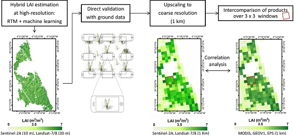
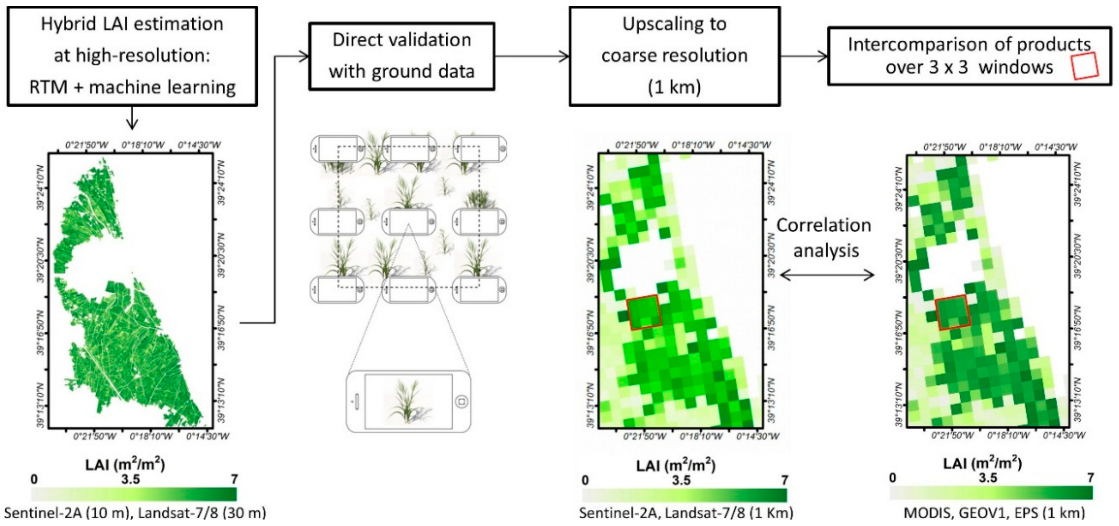
2.1. Methodological Approach

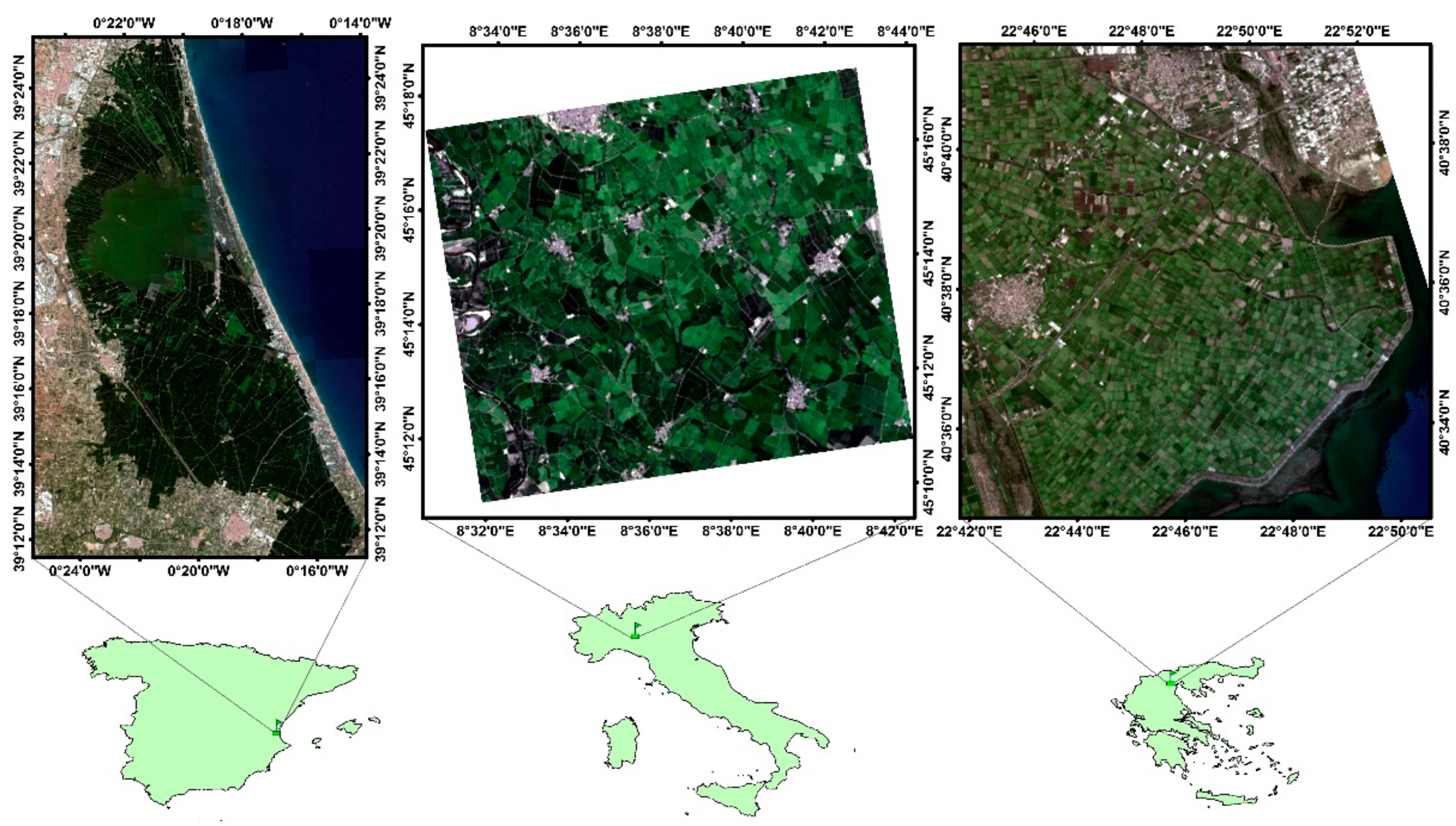
Following international recognized protocols (CEOS LPV guidelines), a multiscale approach is adopted to assess quality of three low-resolution operational LAI products from MODIS (MOD15A2), Copernicus PROBA-V (GEOV1) and the recent EUMETSAT Polar System (EPS). Figure 1 shows a scheme of the comparison procedure that follows four main steps: (1) production of customized decametric satellite products from Landsat-7/8 and Sentinel-2A platforms, (2) direct validation with ground data exploiting representative field sample measurements acquired according to a standardize scheme, (3) upscaling of high-resolution LAI maps to coarse resolution, and (4) exploitation of such data to perform a comparative analysis. A further comparison of moderate-resolution products (i.e., MODIS, GEOV1 and EPS) was conducted by performing a temporal assessment. Temporal dynamics and magnitudes of the three products were analysed for representative rice pixels in order to discuss if the intra-annual variations associated to the phenological cycle were captured.

The following sections describe the study areas (Section 2.2), the field data acquired (Section 2.3), the remote sensing images and product exploited (Section 2.4) and the data analysis conducted for the comparison (Section 2.5).

2.2. Study Areas

The three study areas selected in this work belong to the ERMES FP7 project which aimed at developing a prototype of Copernicus down-stream services assimilating EO and in situ data on crop modelling dedicated to the rice sector. The ERMES study areas were selected in three Mediterranean countries (Spain, Italy and Greece, Figure 2), which are responsible of 85% of total European rice production. The Spanish study area is located within the Albufera Natural Park (Valencia rice district, East of peninsular Spain) that is a special protection area while the Italian study area belongs to the Lomellina rice district (southwestern Lombardy region). In the case of Greece, the study area is located in the Thessaloniki rice district, which is the main cultivation area for Greece. A wide range of rice varieties are cultivated over the study areas covering both Japonica and Indica groups. All study areas belong to temperate rice eco-regions, where a single summer rice cycle can be performed due to climate constraints. Rice sowing is carried out around mid-May in Spain and Greece, whereas in Italy sowing dates may vary from April (for long-cycle varieties—about 150 days from sowing to harvesting) to end of May (modern short-cycle varieties—about 120 days).

In terms of management in the south of Europe, irrigation, fertilization and agro-chemical treatments are performed to guarantee unlimited conditions for rice growth and development. In all three areas fields are irrigated by keeping them flooded for most of the time during the rice-growing period. Italy is the only place where rice is also cultivated via dry seeding with delayed flooding. This practice consists of sowing on dry soil in late April or the beginning of May, keeping the soil moist through short irrigation bouts but not flooded until the unfolding of 2–4 leaves approximately one month after germination, and then flooding the fields from June onward [51]. Fertilisation is generally split in different moments. A pre-sowing Nitrogen-Phosphorus-Potassium (NPK) basal fertilization is generally followed by a first top cover nitrogen fertilisation at tillering (about mid-June) and in some cases by a second top-cover fertilization at panicle initiation (about mid-July). Concerning phytosanitary threats, the main hazard for rice production is related to rice blast (Pyricularia oryza) attacks, which is usually managed through fungicide (e.g., tricyclazole) treatments in July-august according to regional agency bulletins or agro-technical consultant suggestions. Harvesting is performed from late September to October.

2.3. Field Campaigns

Non-destructive PAI_eff ground measurements were acquired with smartphones over the study areas using the PocketLAI app in the framework of the local ERMES field activities. PocketLAI uses both the smartphone’s accelerometer and camera to acquire images at 57.5° below the canopy and compute PAI_eff estimates through an internal segmentation algorithm [35].

Field campaigns over the Spanish and Italian areas were conducted in 2014, 2015 and 2016 throughout the rice phenological cycle; in Greece, only during 2015 and 2016. Based on land cover distribution in the areas and information provided by farmers at the very beginning of the rice season, a reliable sampling was achieved selecting ESUs (Elementary Sampling Units) with different rice varieties and sowing dates in order to cover as much as possible the variability of the study areas.

Table 1. Number of ESUs sampled on the study areas during the 2014, 2015 and 2016 rice seasons.

Rice Season	Number of ESUs
	Spain	Italy	Greece
2014	26	18	-
2015	40	18	10
2016	32	16	10

shows the number of ESUs in which PAI_eff measurements were acquired. The temporal frequency of the campaigns was approximately 7–10 day starting from the very beginning of rice emergence (early-June) up to the maximum PAI_eff development (mid-August). Measurement dates are shown in Tables S1–S3 in Supplementary Materials. The same sampling scheme was used over each ESU, following the VALERI guidelines and recommendations. The size of the ESUs was approximately 20 m × 20 m, and their locations were far from the field borders. A range of 18 to 24 measurements was taken with the goal of characterizing the spatial variability within each ESU, and the ESU centre was geo-located using a Global Positioning System (GPS) for later matching the ground mean LAI measurement with the corresponding remote sensing estimate.

2.4. EO Data and Processing

2.4.1. Remote Sensing High-Resolution LAI Estimates

The high-resolution LAI estimates were produced in the framework of ERMES project. This dataset includes both Sentinel-2A and Landsat-7/8 LAI retrievals. The Sentinel-2A products were recently obtained and validated during the 2016 rice season over the three rice areas [15]. The LAI retrieval approach is based on a hybrid method combining radiative transfer modelling and machine learning regression. In particular, the PROSAIL radiative transfer model [52] was run to simulate rice LAI and associated multispectral reflectances in the corresponding Sentinel-2A bands. This database (composed by LAI-multispectral reflectance data pairs) was then used for training the GPR, which is able to estimate LAI using multi-temporal Sentinel-2A imagery in near real time. In addition, the dataset includes a set of Landsat-7/8 LAI estimates produced in 2015 over Italy and Spain using the same retrieval methodology, but customized for LAI retrieval from Landsat-7/8 features [14]. Finally, the time series of Landsat-7/8 LAI estimates over Italy and Spain for the 2014 and 2016 seasons, and over Greece for the 2015 and 2016 seasons were extended and completed. The validation of these data is provided in Section 3.1.

Table 2. Acquisition dates, shown as day of the year (DOY), of the high-resolution Landsat-7/8 and Sentinel-2A imagery over the study areas.

	Year	Landsat-7/8 DOY	Sentinel-2A DOY
Italy	2014	144,160,184,200,216,256,296	-
	2015	147-155-171-179-187-195-203	-
	2016	142-158-166-174-182-198-214-230-238-246-254-270-278-286	143-173-183-193-203-223-253-263-273
Spain	2014	139-155-171-179-196-203-212-219-227-244-251-283	-
	2015	142-151-158-167-174-182-190-199-215-222-238-246-263-287	-
	2016	146-154-161-170-177-186-193--201-210-217-225-233-241-250-265-282-289	142-162-172-192-212-222-232-242-252-262-282
Greece	2015	141-165-173-189-197-205-213-221-229-237-245-261-277-285	-
	2016	144-152-168-176-184-192-200-216-224-240-248-264-272-288	145-175-183-195-205-215-225-235-245-255-275

shows the remote sensing data acquisition dates for every site and season.

2.4.2. Remote Sensing LAI Products

MODIS (MOD15A2)

Terra MODIS Collection 5 LAI product (MOD15A2) [28] has been produced since February 2000 until March 2017 at eight-day step over a sinusoidal grid at 1 km spatial resolution. The main algorithm of the product is based on a three-dimensional radiative transfer model which links surface spectral bi-directional reflectance factors (BRFs) to both canopy and soil spectral and structural parameters. The algorithm estimates LAI by comparing observed and modelled MODIS BRFs that are stored in biome type specific look up tables. A backup algorithm based on NDVI relationships with LAI [53], calibrated over the same radiative transfer model simulations is used if the main algorithm fails. Both main and back-up algorithms use a biome map in which global vegetation is classified into eight biomes. The product was downloaded from the MODIS data pool (https://lpdaac.usgs.gov/data_access/data_pool) and resized on the study areas for the 2014, 2015 and 2016 rice seasons.

Copernicus PROBA-V (GEOV1)

The Copernicus Global Land Service provides open access, among others, to a LAI product from SPOT/VEGETATION (1999 to May 2014) and PROBA-V (June 2014 up to date) at 1/112° spatial resolution (1 km at the equator) in a Plate Carrée projection (regular latitude/longitude grid), namely GEOV1 products. In this case, the LAI retrieval processing chain relies on neural networks trained to generate LAI estimates by fusing and scaling MODIS c5 and CYCLOPES v3.1 products [19]. The input data of the retrieval chain are top of canopy directional normalized reflectance from either SPOT/VEGETATION or PROBA-V computed using a kernel-driven bidirectional reflectance distribution function (BRDF) model [54]. The retrieval methodology uses a temporal weighting function giving the higher weight in the last observation of the composing period. The estimates are built from 30 days composite observations and the products are provided at a 10 days sampling interval. Similarly to MODIS case, GEOV1 data were downloaded from Copernicus portal (http://land.copernicus.vgt.vito.be) and resized over the three study areas.

EUMETSAT Polar System (EPS)

The Satellite Application Facility (SAF) for Land Surface Analysis (LSA), also known as LSA SAF, is a dedicated processing centre serving EUMETSAT. LSA SAF provides biophysical variables such as LAI which is retrieved from EPS formed by the Meteorological–Operational (MetOp) constellation [31]. MetOp carries a wide range of sensors on-board; among them, the AVHRR instrument is the main sensor in charge of providing observations useful for LAI retrievals. AVHRR offers capability to observe the whole globe every day at 0.01° spatial resolution (at nadir), in the visible and infrared bands of the electromagnetic spectrum. The Land-SAF EPS vegetation products are based on the cloud-free BRDF k₀ parameter [55] of the EPS 10-day albedo product. The LAI retrieval algorithm is based on a hybrid methodology inverting the PROSAIL RTM with multi-output GPR. EPS vegetation products have been computed internally in LSA SAF at 10-day time step from 2015 to present and will be freely available in the next months in near real time at https://landsaf.ipma.pt. In addition, the products will be reprocessed from 2008 onwards.

Table 3. Characteristics of the coarse- (GEOV1, MODIS and EPS) and high-resolution (Landsat and Sentinel-2) LAI products.

	Resolution	Projection	Coverage	Frequency	Compositing	Algorithm
GEOV1	1 km	Plate Carrée (lat/lon)	1999-present (global)	10 days	30 days	Fusion of CYCLOPES & MODIS [19]
MOD15A2	1 km	MODIS sinusoidal	2000-2017 (global)	8 days	8 days	Look-up table inversion of 3D RTM [26]
EPS	1 km	EPS/AVHRR sinusoidal	2015-present (global)	10 days	20 days	GPR based inversion of PROSAIL [31]
Landsat-7/8	30 m	UTM-30N	2014-2016 (study areas)	16 days	-	GPR based inversion of PROSAIL [14]
Sentinel-2A	10 m	UTM-30N	2016 (study areas)	10 days	-	GPR based inversion of PROSAIL [15]

shows the main characteristics of the coarse and high-resolution LAI products.

2.5. Data Analysis

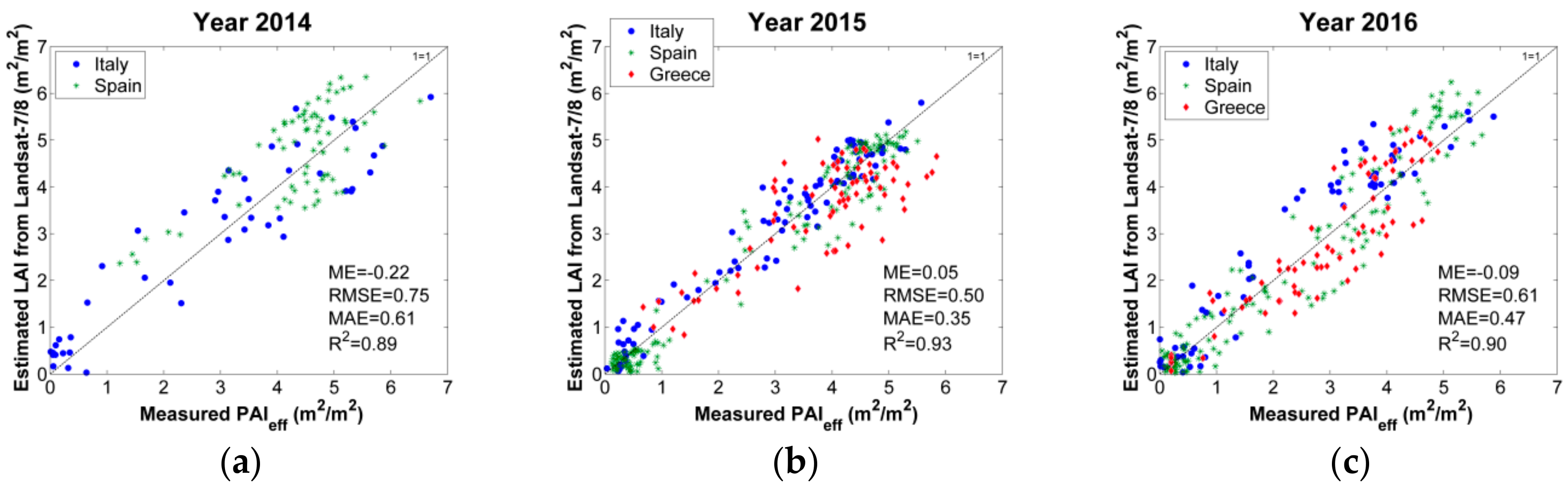
2.5.1. Validation of the Landsat LAI Maps against Ground Measurements

Sentinel-2A LAI maps were already validated as reported in [15]. Following the same approach we first generate LAI maps from Landsat-7/8 and then perform a validation to assess their accuracy. LAI retrievals were obtained at decametric spatial resolution over the three rice areas in different years. In the case of Italy and Spain, Landsat-7/8 LAI estimates were obtained during the 2014, 2015 and 2016 rice seasons while in the Greek study area the estimates were obtained and assessed in 2015 and 2016. The mean error (ME), root mean squared error (RMSE), mean absolute error (MAE), and coefficient of determination (R²) were computed in order to assess accuracy, bias and goodness-of-fit between LAI retrievals and the corresponding in situ measurements (see metrics in Table S4).

In addition, the retrieved LAI maps were compared with results obtained using pure statistical methods based on a transfer function (TF) recommended by CEOS LPV for validation of biophysical products. Following previous studies [36,40,56,57], the multivariate ordinary least squares (OLS) regression based on iteratively re-weighted least squares (IRLS) method was used to establish a relationship between the average PAI_eff measurements from each ESU and the corresponding multispectral data from high-resolution data, in our case Landsat-7/8 data.

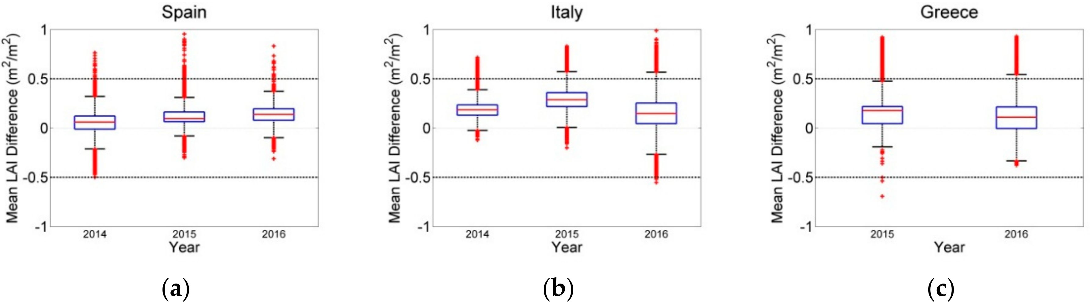
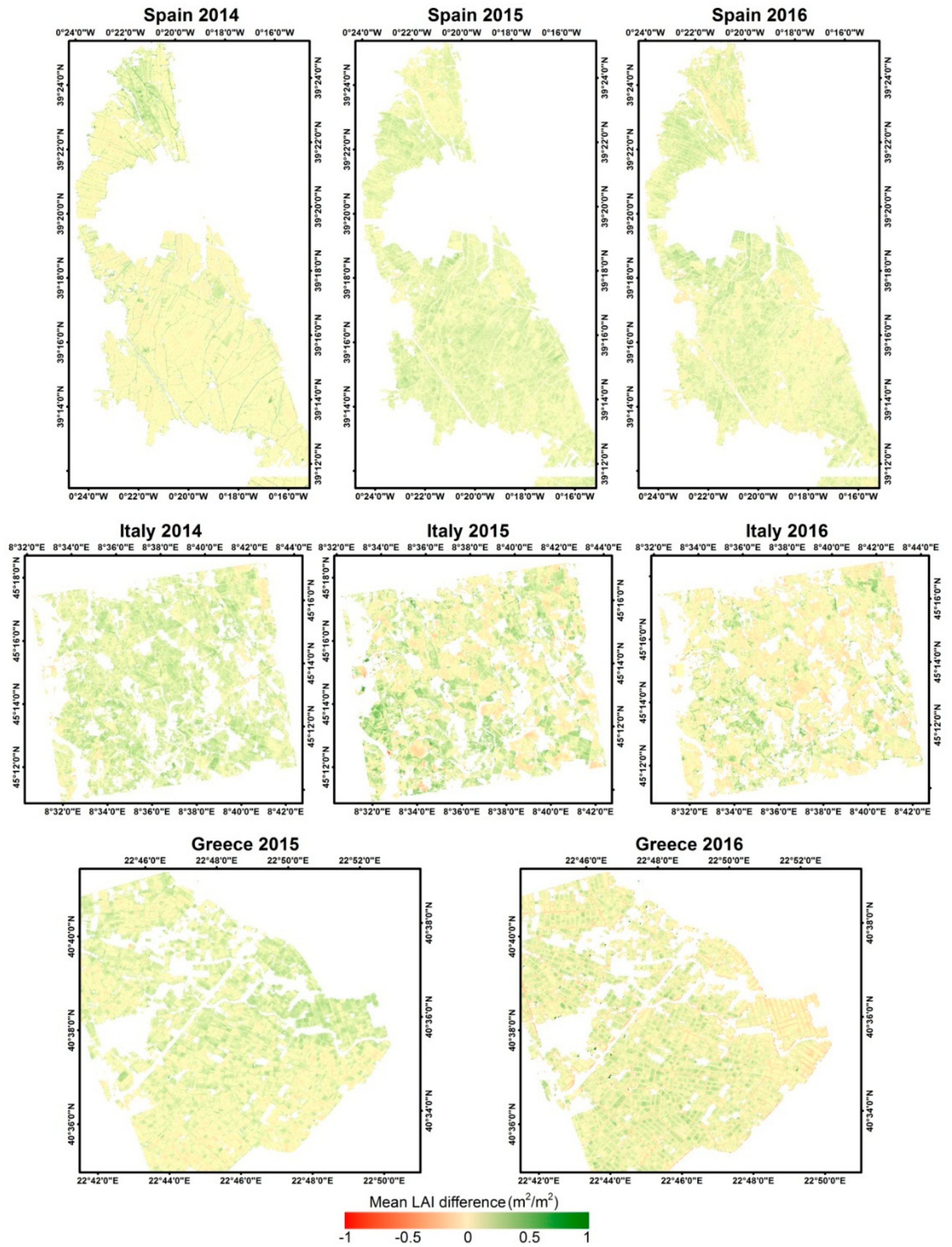
2.5.2. Comparison of Coarse- and High-Resolution LAI Estimates

Since the low- and high-resolution maps to be compared differ in spatial and temporal resolutions, the comparison was conducted for the closest dates of each product at a lowest spatial resolution to minimize differences due to a spatial–temporal mismatch [47]. As different temporal compositing schemes are considered in the satellite products (Table 3) each product was associated with the central value of its temporal window. The comparison between pairs of products considered only good quality observations of the closest central date. All LAI maps were resampled to the GEOV1 1 km regular latitude/longitude projection in order to assure the same projection for all products. Subsequently, the comparison was achieved by averaging the LAI values over a window of 3 × 3 pixels if more than five out of the nine pixels were valid in order to reduce misregistration errors between images and inconsistencies associated to differences in the Point Spread Function (PSF) of the respective sensors [44]. Quality information provided by products’ quality flag was used to filter pixels flagged as invalid or poor quality. Similarly to Section 2.5.1, The ME, RMSE, and R² were computed in order to assess accuracy, bias and goodness-of-fit between products.

3. Results

This section is devoted to assess the Landsat-7/8 LAI estimates obtained by means of applying the hybrid retrieval (i.e., PROSAIL inversion with GPR) in 2014, 2015 and 2016 with in situ data acquired during every season. In addition, we also undertake a comparison exercise between the high-resolution and moderate-resolution LAI products over the study areas in order to evaluate its consistency.

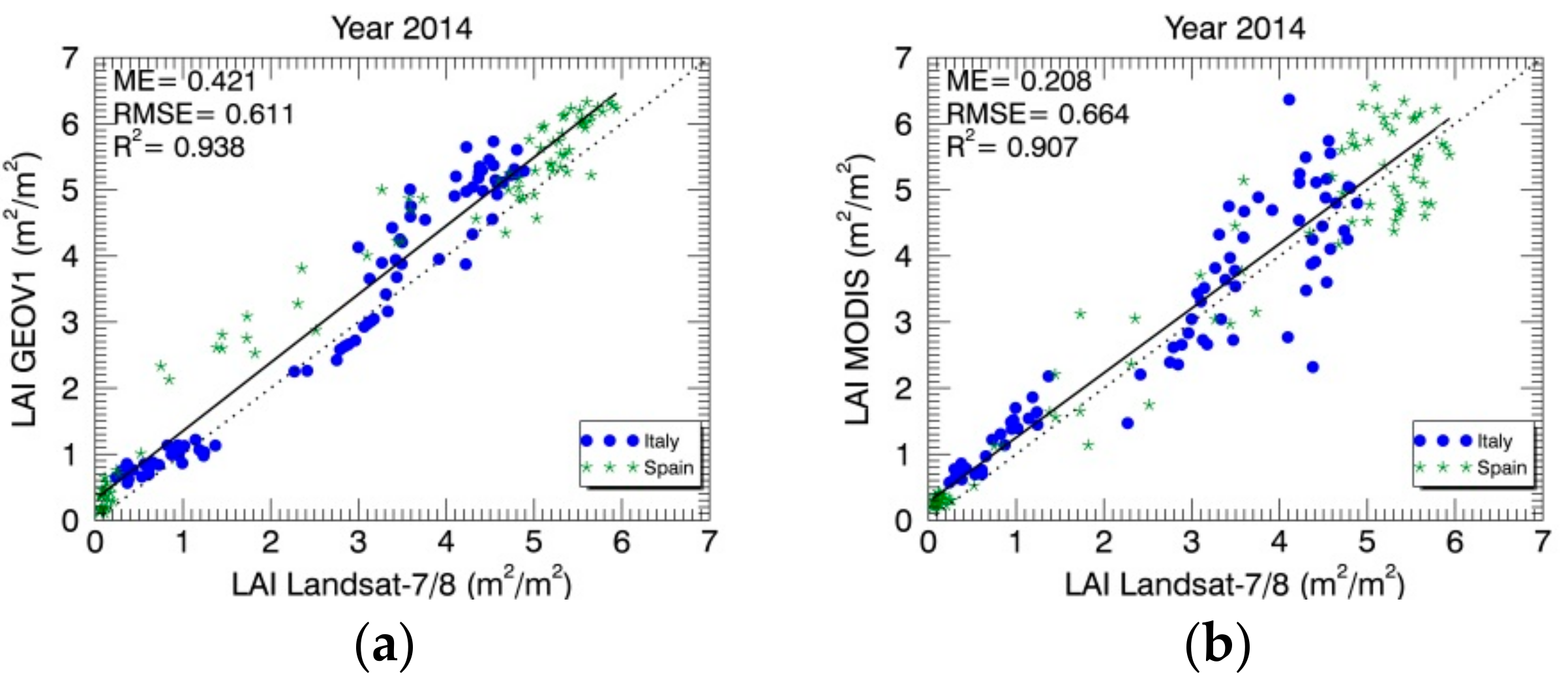
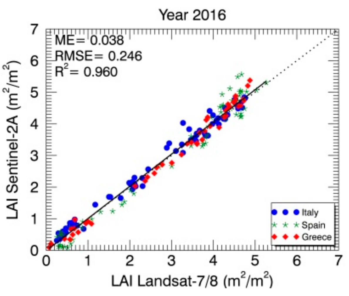
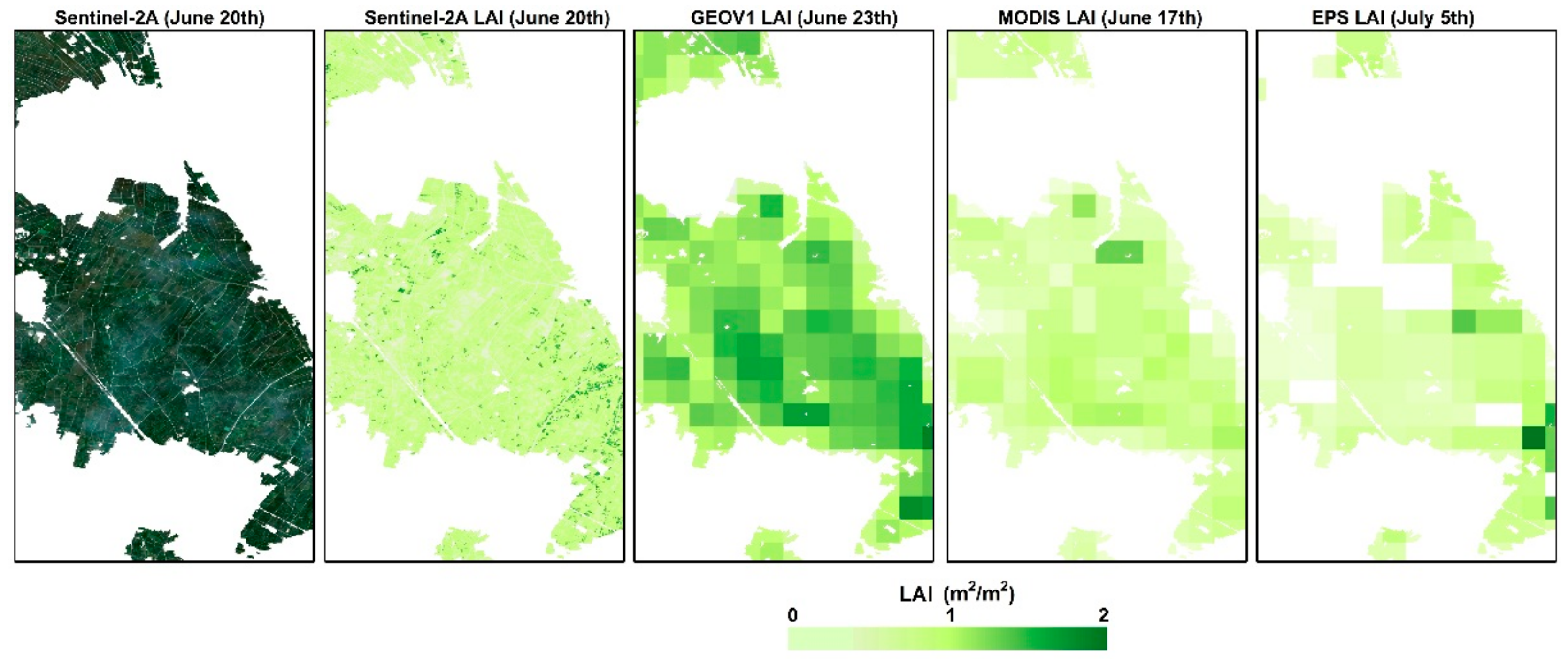
3.1. Assessment at High Spatial Resolution

Figure 3 shows the results of validation exercise for Landsat-7/8 LAI when compared with field data acquired in three years in all three locations. High correlations (R² ≥ 0.89), low errors (RMSE in the range 0.50–0.75 m²/m² and MAE in the range 0.35–0.61 m²/m²) and biases (ME = −0.22, 0.05, and 0.09 m²/m² in 2014, 2015 and 2016, respectively) are found, which highlights the consistency between Landsat-7/8 estimates and ground measurements. These results are in accordance with the accuracy of LAI retrievals obtained in 2016 over the same rice areas using Sentinel-2A imagery [15].

Figure 4 shows the seasonal mean LAI difference maps between the retrieved LAI maps (e.g., RTM inversion) and ground based LAI maps obtained with the TF. In general, the hybrid retrieval produces slightly higher mean values in all rice areas. However, the vast majority of pixels fall within the range of ±0.5 m²/m² which highlights the high correspondence between maps (Figure 5). Slightly greater differences were found in Italy. This can be explained by the higher variability of the study area in terms of cultivated varieties, agronomic practices (dry vs. water sowing) and sowing dates.

The good performance found when comparing Landsat-7/8 and Sentinel-2A LAI retrievals with ground measurements as well as the high consistency between the outputs of the RTM inversion method and the statistical TF maps, justify their use as reference maps for the assessment of coarse-resolution LAI products over rice areas.

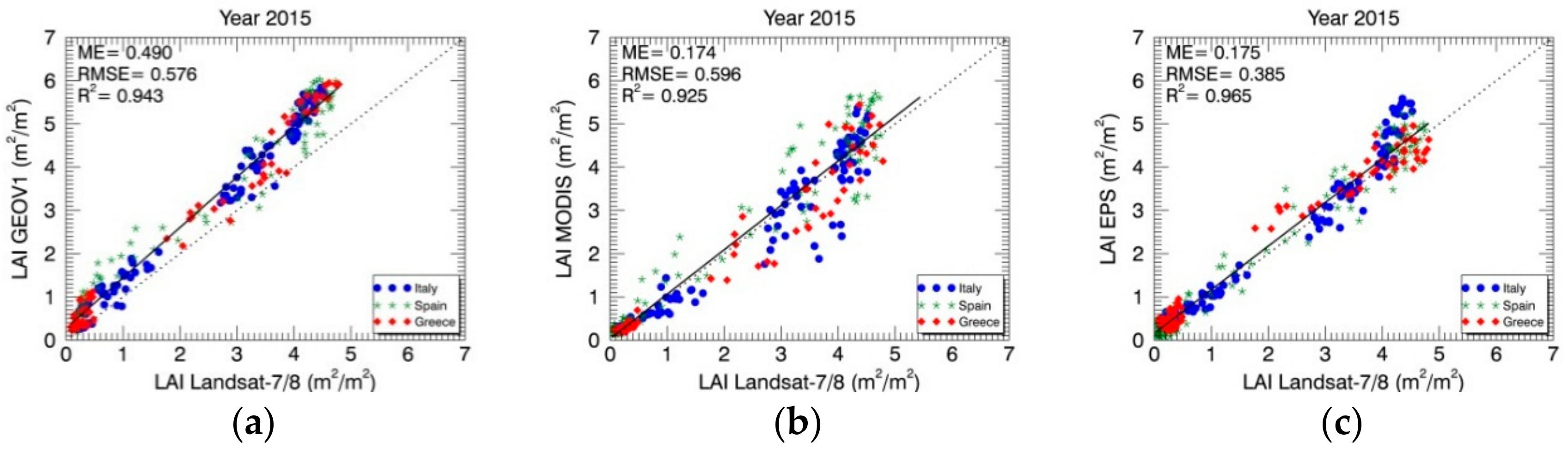
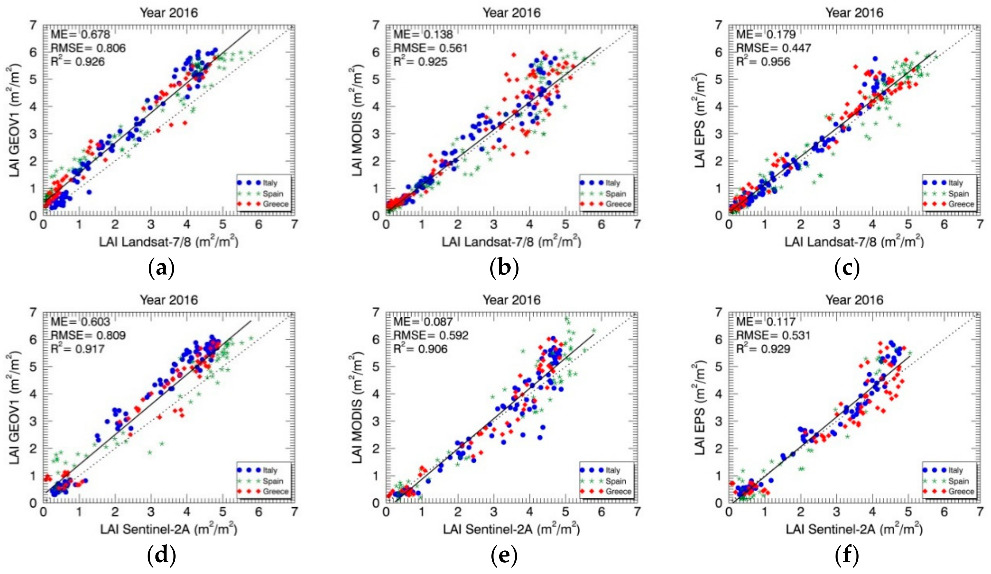
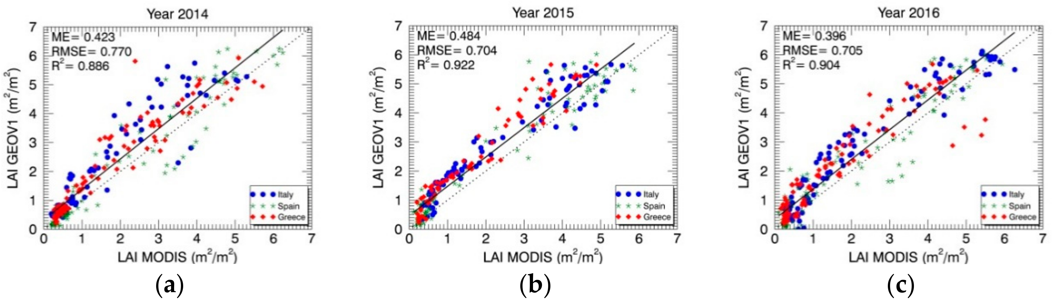
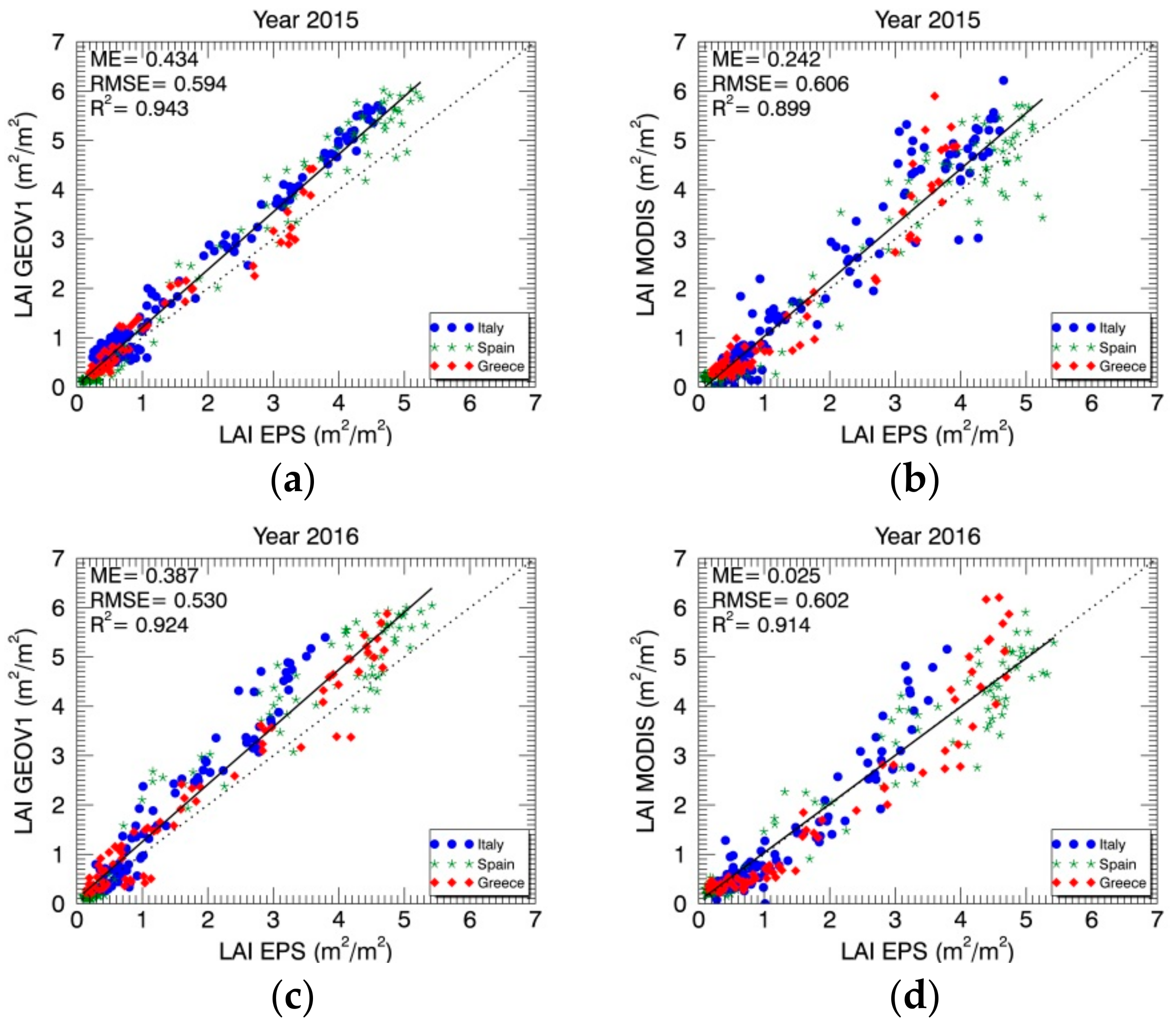
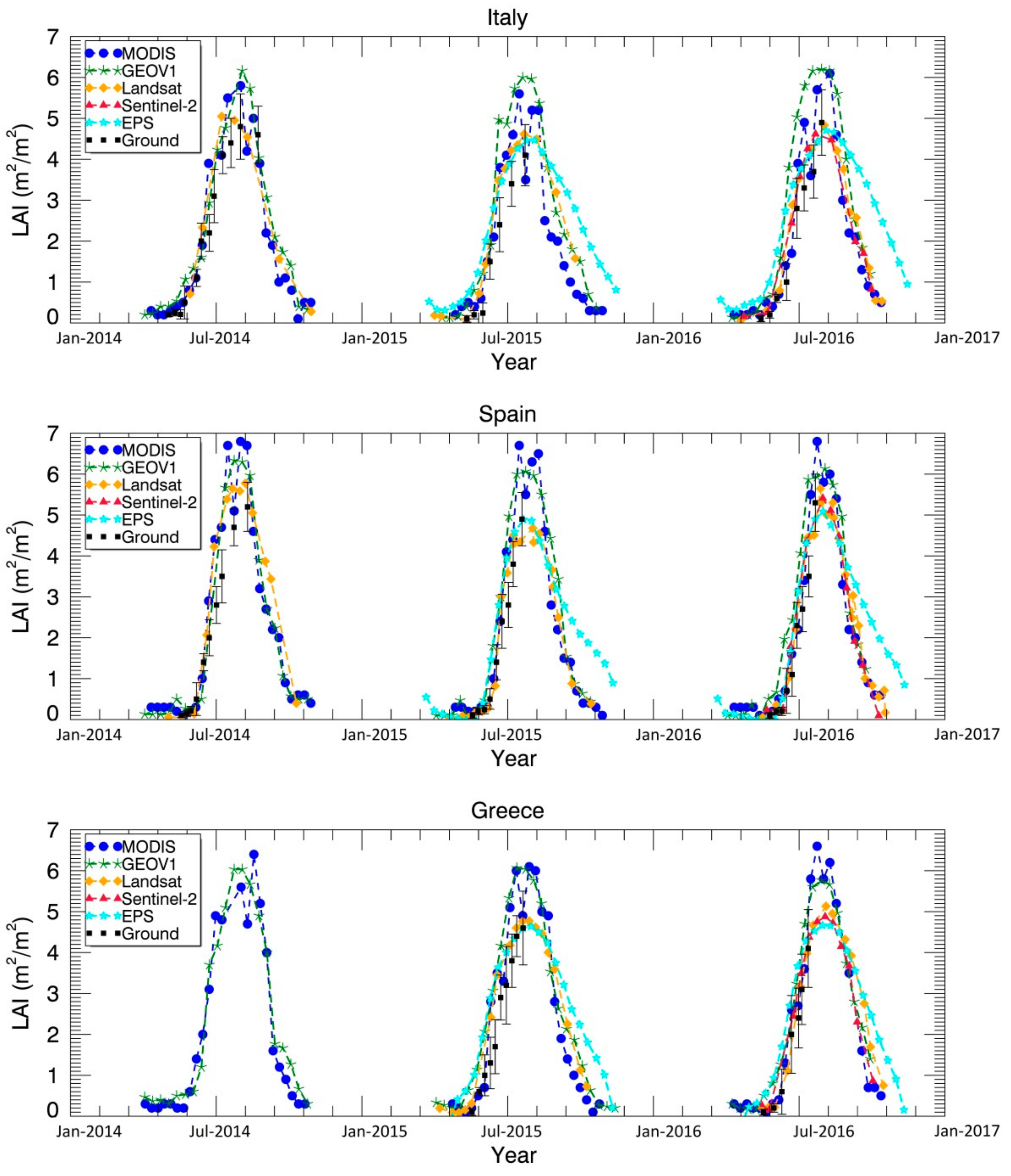
3.2. Analysis of Accuracy of Coarse-Resolution LAI Maps

The next step was to compare both the Landsat-7/8 and Sentinel-2A LAI estimates (upscaled at 1 km spatial resolution) with the coarse satellite LAI products (MODIS, GEOV1 and EPS). In order to assess the consistency between estimates from Sentinel-2A and Landsat, a scatterplot of aggregated values for corresponding dates during year 2016 is shown in Figure 6. A good correspondence (R² = 0.96, RMSE = 0.25 m²/m²) and practically no bias is observed. Figure 7, Figure 8 and Figure 9 show the scatterplots between the products in the 2014, 2015 and 2016 rice seasons, respectively. In general, the GEOV1, MODIS and EPS LAI products fit well with the aggregated estimates derived from the high-resolution ones as proved by a coefficient of determination higher than 0.9 in all cases. In 2014, GEOV1 estimates present higher correlation and similar RMSE than MODIS with regard to Landsat-7/8 upscaled estimates (Figure 7). Note that in 2014 no EPS and no Sentinel-2A data were available. In 2015, EPS estimates were the most correlated with Landsat-7/8. In 2016, EPS is the most correlated with both Landsat-7/8 and Sentinel-2A upscaled LAI retrievals, also revealing lower errors and biases with respect to GEOV1 and MODIS (Figure 8 and Figure 9). A significant good agreement is found between EPS and Landsat-7/8, with R² = 0.97, RMSE = 0.39 m²/m², and ME = 0.18 m²/m² in 2015, and R² = 0.96, RMSE = 0.45 m²/m², and ME = 0.18 in 2016.

GEOV1 products present a slight overestimation (up to 0.7 in LAI units) regarding Landsat-7/8 and Sentinel-2A products for all the years and sites, although with very high correlation values (R² > 0.91 in all cases). MODIS estimates present also a good correlation (R² > 0.90) and lower bias (ME < 0.2) with Landsat-7/8 and Sentinel-2A products (Figure 7, Figure 8 and Figure 9).

In addition, a comparison was conducted among the satellite LAI products over the study areas. Figure 10 shows the scatterplots of GEOV1 versus MODIS for the three seasons. Both products present reasonably high correlation (R² ≥ 0.88) and moderate differences (RMSE ≤ 0.70 m²/m²; ME ≤ 0.50 m²/m²) in the three years. A similar comparison was also conducted during 2015 and 2016 using the available EPS product (Figure 11), which revealed a high consistency among products (R² ranging from 0.90 to 0.94, RMSE ≤ 0.61 m²/m² and ME ≤ 0.44 m²/m² in all cases). The EPS LAI estimates are found to be similar to those of MODIS and GEOV1 products in the first stages of rice growth, while EPS seems to produce consistently lower LAI values, with biases that reach up to 1 m²/m² for dense canopies, particularly when compared with GEOV1.

Figure 12 shows LAI time series for the three rice seasons as obtained by averaging all valid observations within a window of 2 km × 2 km where the typical rice plant phenological cycle of each study area is captured. Ground measurements falling within the window are also provided as a reference, even though they are not directly comparable due to scaling effects. Note that in 2014, Landsat-7/8 LAI estimates were not provided over the Greek rice area since no ground data were available. All products captured similarly the rice LAI temporal evolution showing the highest values in mid-August (peak of season). Over this window, EPS seems consistently lower than MODIS, while the regression results for 2016 suggest that on average they are similar. There is a significant difference in the amplitude of the LAI curve between MODIS and GEOV1 and the rest of products (F ≈ 5 and p < 0.01 in all cases). Both products present a LAI peak of season of around 6 m²/m², while EPS, Landsat-7/8 and Sentinel-2A reach maximum values of about 5 m²/m².

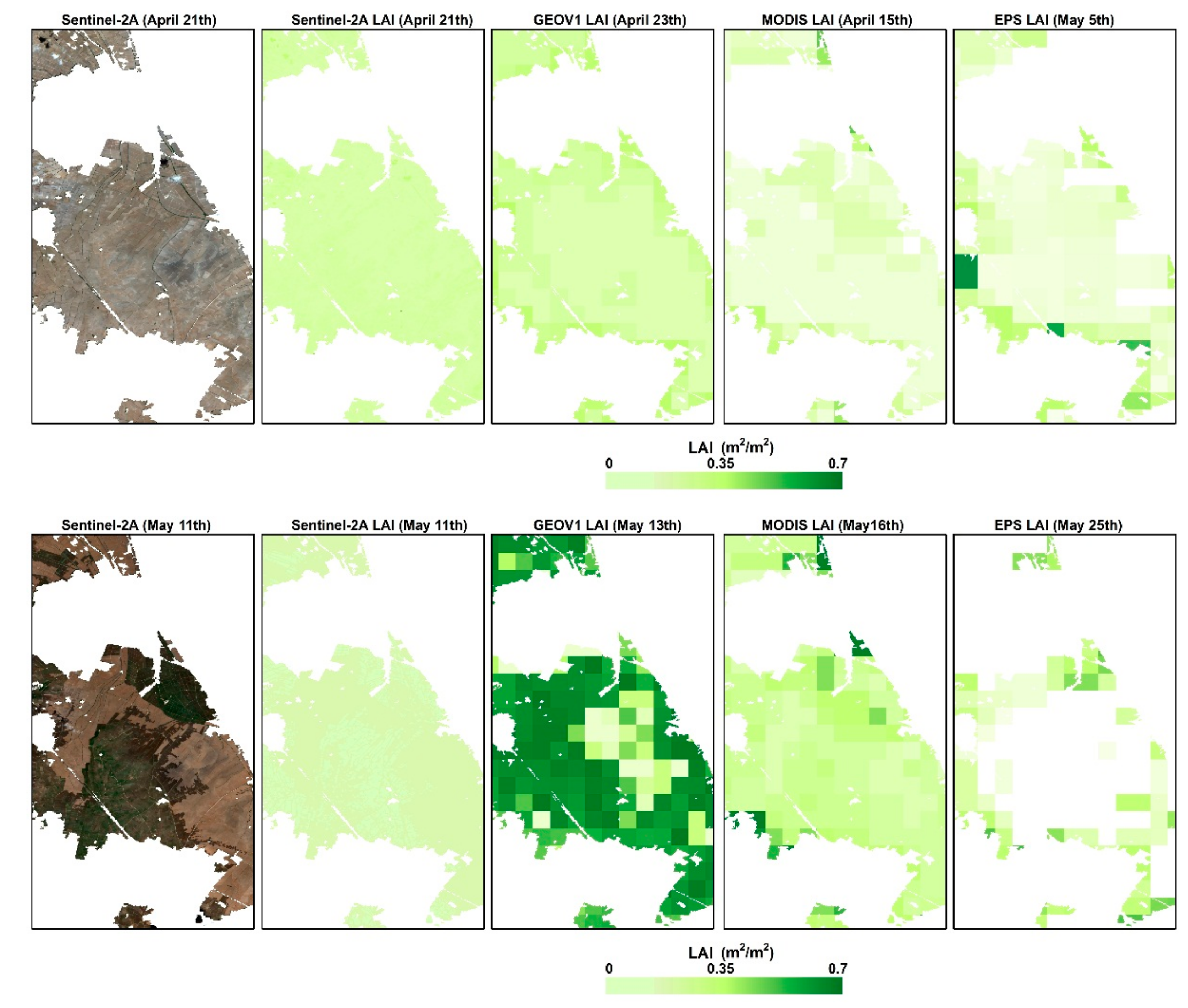
3.3. Influence of Flooding Conditions in LAI Retrievals

One of the main characteristics of rice cropping systems is the rice soil background condition which can be flooded most of the time during the season. This may introduce difficulties in LAI estimation from remote sensing (RS) data in the first part of the season, when canopy closure is low and flooding conditions strongly affect the detected signal. The performances of both the HR and the three coarse-resolution LAI products in these difficult conditions are exemplified in Figure 13, which shows the results obtained in the very first stages of the season in the Spanish rice area in 2016. Note that the apparent inconsistency in the dates between the three coarse-resolution products of Figure 13 is related with the significant differences in the timeslot of file names: for EPS, the timeslot corresponds to the last day of the 20-day time-compositing period; for MODIS to the first day of the 8-day period; and for GEOV1 to the 13th day of the 30-day compositing period.

Both Landsat-7/8 and Sentinel-2A LAI estimates take into account rice background spectra (flooded and non-flooded) in PROSAIL simulations and provide very low/zero LAI values in dry bare soil or in water during the sowing and pre-sowing period. Concerning coarse-resolution products, all of them showed values virtually zero in mid-April (Figure 13, top panel) when the soil was dry, which is coherent with the visual inspection of the area. Some unrealistically high LAI values can be observed on the borders of the study area, in particular for the EPS product: these are, however, mostly a consequence of the large LAI differences existing during May between the bare rice areas and the surrounding land cover, dominated by orange trees. In these conditions, sensors’ PSF (Point Spread Function) effects may lead to contamination of the signal for the borders’ pixel and consequently to positive errors in LAI retrieval. These border effects in LAI patterns are in fact more significant in the case of EPS due to the larger field of view of AVHRR.

Results of a similar comparison based on LAI maps related to the second decade of May show instead very different results (Figure 13, middle panels). The high-resolution Sentinel-2A images revealed that rice fields started to be flooded around the first decade of May (information verified by farmers). The GEOV1 LAI product of 23 April, based on PROBA-V observations of 1 May to 30 May, presented unrealistic high estimates (i.e., 0.4–0.7 m²/m²), particularly in the first flooded fields. This may be a major limitation leading to improper (too early) estimations of the start of the season. The EPS product, though not showing such an overestimation, presents large NoData areas in correspondence of the central part of the study area. The reason for this is that the EPS algorithm applies empirical thresholds to mask areas characterized by the likely presence of undetected snow, inland water, and large input errors or out of physical ranges in reflectance values [31]. In particular, reflectance of flooded soils cause unrealistic inputs (very dark reflectance pixels) leading to missing observations. The bottom panel of Figure 13 (related to LAI estimates corresponding roughly to the end of June) highlights again a tendency towards overestimation for the GEOV1 LAI product, while both MODIS and EPS provide more realistic values close to the Sentinel-2A LAI estimates, showing thus to be more robust against changes in rice background conditions. The overestimation of the GEOV1 LAI product can be explained in the fact that the dark background spectra under flooded conditions is not considered in the RTM simulations of the CYCLOPES products, which has a large impact on the GEOV1 training for low LAI values [19,29].

4. Discussion

In this work we used customized high-resolution LAI maps, produced by RTM inversion for rice-cultivated areas, as reference maps to analyse the quality, accuracy and consistency of satellite LAI products. There are several foundations for exploiting optimally trained RTM inversion methods as an alternative for the widely accepted TF approach: (1) a TF linking field measurements with high-resolution remote sensing is constrained by the number of ESUs, requiring typically 50 to obtain accurate results; (2) pure statistical methods could be biased if ground measurements were not sampled properly since they are not able to extrapolate the ranges seen in the ground dataset (i.e., out of the convex hull), whereas in hybrid approaches a broad range of vegetation situations can be addressed, leading to a dataset covering wider LAI ranges. Thus, suboptimal ground sampling could lead to spatial errors and inconsistencies; (3) linear TFs could not describe properly the well-known non-linear relationship between LAI and reflectance, while RTM approaches rely on physical basis of how radiation interacts with foliage and passes through vegetation canopy to produce the remotely measured signal. On the other hand, the use of the RTM approaches are also limited by the model assumptions on background and canopy spectra, and canopy structure, and should be properly calibrated for a specific region and validated before using them as a validation reference.

The decametric maps produced from Landsat-7/8 data through the developed inversion of RTM with GPR provided RMSEs values (0.75, 0.50 and 0.61 m²/m² for 2014, 2015 and 2016, respectively) comparable to results previously obtained with real Sentinel-2A data [15], and outperformed previous LAI retrieval studies over rice areas using PROSAIL LUT inversion (RMSE = 2.26 m²/m²) [58]. Similar accuracy in LAI retrievals has been reported using LUT inversion of PROSAIL over other cereal crops, e.g., RMSE = 0.9 m²/m² over maize [59] and RMSE of 0.42 and 0.64 m²/m² over maize and wheat respectively [60]. In addition, these HR LAI estimates are highly consistent with PocketLAI measurements. Since previous studies have reported a slight negative bias in PocketLAI measurement over rice regarding LAI-2000 and DHP, a slight underestimation could be present in HR LAI estimates, mainly when canopy closure is high due to saturation effects.

Water background showed an impact on LAI retrievals mainly in the very beginning of the rice season. Both Landsat-7/8 and Sentinel-2A LAI showed good accuracy in the first stages of the season. An alternative to PROSAIL would be the use of SAILHFlood [61], which was specifically designed for simulating partial submerged canopy. SAILHFlood is a modification of SAILH RTM in which the emerged vegetation layer and the submerged vegetation layer are simulated, thus accounting for both emerged and submerged LAI. However, SAILHFlood assumes vegetation to be submerged into clear water, which is not very likely to occur on rice crops. Future research could include the coupling of SAILHFlood with leaf-level RTM (e.g., PROSPECT) to account for both canopy and leaf levels over partially submerged canopies.

In general, the three satellite products (MODIS, GEOV1, and EPS) fit well with the aggregated decametric LAI maps and presented good correspondence and consistent seasonality among them. Although an overall positive offset is found for these products (primarily GEOV1), this bias is small and may be partly compensated with the possible negative bias pointed out for the decametric LAI estimates. Highlighted differences (more evident for high values) are partly due to the different algorithms used for LAI estimation (e.g., temporal compositing windows), the different LAI definition used, sensor spectral response and point spread function, or the use of different atmospheric correction methods [45,47,62,63]. The MODIS LAI retrieval approach accounts for vegetation clumping at leaf and canopy scales through radiative transfer formulations, so that estimated values should be closer to actual (rather than effective) LAI. In turn, GEOV1 algorithm is trained based on the fusion of MODIS c5 and CYCLOPES v3.1 products [64], using a weighted combination that is closer to CYCLOPES v3.1 LAI products for low-medium LAI values and closer to MODIS for dense canopies. GEOV1 is thus closer to an effective LAI for low values. MODIS and GEOV1 agree well because they rely on similar approaches and should be both closer to actual LAI for high values during summer [64]. On the other hand, EPS relies on a turbid radiative transfer model, which does not account for clumping effects. EPS estimates are thus lower in summer, but more similar to Sentinel-2A, and Landsat-7/8 LAI estimates, which rely on similar hybrid LAI retrieval methods and should be closer to an effective LAI. Differences in LAI definitions could explain why during the first stages of the phenological cycle (low and medium LAI values) the temporal evolution of products is more consistent than during the peak of season, since MODIS and GEOV1 show a wider range in all areas.

With regard to smoothness of the retrieved LAI time series GEOV1 and EPS show smoother temporal evolution than MODIS, which exhibits unrealistic drops in time previously reported in other biomes [20,50,65]. This is reasonably due to the shorter (eight days) compositing period used by MODIS, which can lead to rather strong errors due to unfavourable atmospheric conditions (i.e., persistent cloudiness leading to the use of low-quality/high acquisition angle data as the basis for the retrieval). In general, the LAI products present a sharp drop with values close to zero during the senescence. However, the EPS product presents a smooth rice season ending, suggesting that the product may be more sensitive to residual photosynthetic activity in senescent or dying leaves. In addition, discrepancies in temporal variations are also affected by the compositing period of the product [66]. This effect is more noticeable in the first growing stages of rice, and consequently LAI increases rapidly.

The coarse-resolution satellite products may provide unrealistically high LAI values, particularly in the case of GEOV1, which reaches up to 0.7 m²/m² after the flooding and presents abnormally high values during June. A main limitation of GEOV1 is that it has been designed to characterize the main spectral properties of bare soils but it fails to characterize the typical signatures of flooded fields, causing a large overestimation in flooding conditions during the first crop development stages. This early LAI increase would determine an unrealistic estimate of crop growth and a wrong inference of the emergence date. The effect of water background on rice reflectance anisotropy is in fact minimized as rice plant grows [67] and episodes of water background treatment (drain out water and flood) are less influential when LAI and canopy closure are high. Conversely, the EPS LAI product shows incomplete coverage from flooding to the first stages of rice development since very dark pixels are masked out by the retrieval algorithm.

In summary, from an operational point of view the characteristics of both the high- and low-resolution LAI maps here presented and validated allows their exploitation as a valuable input source for agronomic monitoring. In particular, the HR maps generated from Landsat-7/8 and Sentinel-2A may provide data of utmost importance for local scale studies devoted to provide information about crop status at parcel or sub-parcel scale. Dense time series of HR LAI data can be used to monitor the grow cycle and identify within field anomaly in crop conditions due to the effects of plant diseases or other factors [12]. These data can also be used for phenological retrieval at parcel scale [68] and as input for crop modelling to map yield variability within field [69].

A possible limitation of this dataset is related to the fact that they provide estimates of effective LAI rather than actual LAI. This could limit their usefulness for quantitative applications that require actual LAI estimates. This problem could however be reduced by applying appropriate correction factors based on a comparison of the RS-based LAI product related to actual LAI, or on literature data concerning typical clumping factors for rice at different phenological stages.

Concerning the coarse-resolution products, their usefulness relies primarily in providing valuable data for regional applications such as large-scale crop status monitoring and yield estimation. Besides for “direct” mapping studies, these products can be also of value as inputs for crop modelling studies. This have been already demonstrated during the pre-operational activities of the ERMES project, where low-resolution data derived by aggregating the GEOV1 on a 2 km × 2 km regular grid were assimilated in the Water Accounting Rice Model (WARM) crop model to provide seasonal estimates of rice yield at district scale [12,69]. The EPS LAI maps share the same possible problem of representing an effective LAI value illustrated above for HR products. EPS LAI maps also show a possible overestimation tendency towards the end of the season, which could hamper their usefulness for monitoring late phenological stages and assess metrics such as growing season length. Conversely, the GEOV1 LAI product provides apparently reliable estimations on later stages of the growing cycle, but shows a tendency towards overestimation on the earlier stages, when flooded background seems to affect its reliability. Finally, the MODIS product provides generally consistent estimates throughout the season, its main drawback consisting in a noisier signal. This problem could be however reduced by implementing appropriate smoothing procedures.

In general, the usefulness of these products consists primarily in providing valuable data for regional crop monitoring applications. Besides their usefulness as input for monitoring systems devoted to assess crop condition, these products can be also of value as inputs for crop modelling studies. This have been already demonstrated during the pre-operational activities of the ERMES project, where low-resolution data derived by aggregating the GEOV1 on a 2 km × 2 km regular grid were assimilated in the Water Accounting Rice Model (WARM) crop model to provide seasonal estimates of rice yield at district scale [12,70]. In these studies, it was found that regional yield estimation benefits from exogenous LAI inclusion in crop modelling. A yield forecast system (ERMES-WARM) was developed by simulating fourteen years (2002–2015) of rice related model outputs and adopting proper post processing statistical technique to define multivariate predictive relations with official statistics. The ERMES regional modelling solution was able to explain about 70% of interannual variability of official yields, with Mean Absolute Error in cross validation of 0.12 (Italy), 0.20 (Spain), and 0.30 (Greece) ton·ha⁻¹ [12]. The assimilation of LAI data was demonstrated to improve the model results when compared to reference yield data [70].

5. Conclusions

In this study, high-resolution LAI maps generated from decametric EO data and coarse-resolution operational LAI products were compared over three European rice areas during three rice seasons. At high resolution this study used a set of existing multi-temporal Sentinel-2A LAI estimates as well as three seasons of Landsat-7/8 estimates derived in the framework of ERMES project which have been produced through RTM inversion.

The validation of HR estimates was successfully performed using LAI ground measurements acquired during three rice growing seasons in the three rice areas. Results revealed a satisfactory accuracy of retrieved LAI values and also a good consistency with maps obtained with the standard OLS transfer function methodology along the seasons and sites. This suggests that RTM inversion can be a valuable and cost-effective alternative to typical transfer function approaches, but needs to be well calibrated and validated for a specific area prior to use it as a validation reference. This could result in a reduction of field work that is needed for the empirical approaches.

Both the Landsat-7/8 and the Sentinel-2A LAI estimates were then compared with widely used and validated LAI products such as the MODIS and GEOV1, as well as with the recent EPS LAI product. EPS was the most correlated product with both decametric estimates. GEOV1 LAI products showed slightly higher values with respect to the resampled high-resolution estimates; however, good correlations and low errors were found in all years and sites. An additional comparison was conducted among the satellite LAI products revealing GEOV1 and EPS as the most correlated. Despite the spatial and temporal differences that hamper the comparison among products, the seasonal trends of the LAI products were similar along the seasons. The discrepancies found at high LAI values are partly due to product definition (i.e., actual vs. effective LAI) and retrieval algorithm assumptions. These discrepancies may limit the usefulness of the satellite product as input for crop modelling approaches such as those based on simple radiation use efficiency model, or on assimilation of RS data in crop growth models that exploit a forcing approach. Crop modelling approaches based on the assimilation of RS data through recalibration of model parameters (such as the WARM-ERMES approach used in [12,69,70]) would instead be less sensitive to this constraint. Recalibration techniques of LAI estimates could also be exploited to reduce the problem.

At low LAI values, global LAI products do not seem to always properly characterize water surfaces in rice fields and are thus less robust against changes in background condition related to water management. This problem was found to particularly affect the GEOV1 product, with MODIS and EPS showing higher robustness and therefore being more useful for monitoring the first stages of the growing cycle.

In conclusion, operational coarse-resolution and customized high-resolution LAI products are nowadays in our opinion mature enough to contribute to user community in supporting proper agro-monitoring downstream services as already demonstrated in Europe. In the future, similar assessment will be extended to rice districts located in other continents such as Asia to confirm positive results obtained in temperate areas and investigate potential limitation in tropical condition due to impact of cloud contamination on optical data.

References

1. Turner, D.P.; Cohen, W.B.; Kennedy, R.E.; Fassnacht, K.S.; Briggs, J.M. Relationships between leaf area index and Landsat TM spectral vegetation indices across three temperate zone sites. Remote Sens. Environ. 1999, 70, 52–68. [Google Scholar] [CrossRef]
2. Zhu, Z.; Piao, S.; Myneni, R.B.; Huang, M.; Zeng, Z.; Canadell, J.G.; Ciais, P.; Sitch, S.; Friedlingstein, P.; Arneth, A.; et al. Greening of the Earth and its drivers. Nat. Clim. Chang. 2016, 6, 791–795. [Google Scholar] [CrossRef]
3. Nemani, R.; Pierce, L.; Running, S.; Band, L. Forest ecosystem processes at the watershed scale: Sensitivity to remotely-sensed leaf area index estimates. Int. J. Remote Sens. 1993, 14, 2519–2534. [Google Scholar] [CrossRef]
4. Plummer, S.E. Perspectives on combining ecological process models and remotely sensed data. Ecol. Model. 2000, 129, 169–186. [Google Scholar] [CrossRef]
5. Asner, G.P.; Scurlock, J.M.; Hicke, J.A. Global synthesis of leaf area index observations: Implications for ecological and remote sensing studies. Glob. Ecol. Biogeogr. 2003, 12, 191–205. [Google Scholar] [CrossRef]
6. Allen, R.G.; Pereira, L.S.; Raes, D.; Smith, M. Crop Evapotranspiration-Guidelines for Computing Crop Water Requirements-FAO Irrigation and Drainage Paper 56; FAO: Rome, Italy, 1998. [Google Scholar]
7. Duchemin, B.; Hadria, R.; Erraki, S.; Boulet, G.; Maisongrande, P.; Chehbouni, A.; Escadafal, R.; Ezzahar, J.; Hoedjes, J.C.B.; Kharrou, M.H.; et al. Monitoring wheat phenology and irrigation in Central Morocco: On the use of relationships between evapotranspiration, crops coefficients, leaf area index and remotely-sensed vegetation indices. Agric. Water Manag. 2006, 79, 1–27. [Google Scholar] [CrossRef]
8. Barr, A.G.; Black, T.A.; Hogg, E.H.; Kljun, N.; Morgenstern, K.; Nesic, Z. Interannual variability in the leaf area index of a boreal aspen-hazelnut forest in relation to net ecosystem production. Agric. For. Meteorol. 2004, 126, 237–255. [Google Scholar] [CrossRef]
9. Dietz, J.; Hölscher, D.; Leuschner, C. Rainfall partitioning in relation to forest structure in differently managed montane forest stands in Central Sulawesi, Indonesia. For. Ecol. Manag. 2006, 237, 170–178. [Google Scholar] [CrossRef]
10. Fang, H.; Liang, S.; Hoogenboom, G.; Teasdale, J.; Cavigelli, M. Corn-yield estimation through assimilation of remotely sensed data into the CSM-CERES-Maize model. Int. J. Remote Sens. 2008, 29, 3011–3032. [Google Scholar] [CrossRef]
11. Fang, H.; Liang, S.; Hoogenboom, G. Integration of MODIS LAI and vegetation index products with the CSM–CERES–Maize model for corn yield estimation. Int. J. Remote Sens. 2011, 32, 1039–1065. [Google Scholar] [CrossRef]
12. Busetto, L.; Casteleyn, S.; Granell, C.; Pepe, M.; Barbieri, M.; Campos-Taberner, M.; Casa, R.; Collivignarelli, F.; Confalonieri, R.; Crema, A.; et al. Downstream services for rice crop monitoring in Europe: From regional to local scale. J. Sel. Top. Appl. Earth Observ. Remote Sens. 2017, 10, 5423–5441. [Google Scholar] [CrossRef]
13. Fang, H.; Liang, S.; Kuusk, A. Retrieving leaf area index using a genetic algorithm with a canopy radiative transfer model. Remote Sens. Environ. 2003, 85, 257–270. [Google Scholar] [CrossRef]
14. Campos-Taberner, M.; García-Haro, F.J.; Camps-Valls, G.; Grau-Muedra, G.; Nutini, F.; Crema, A.; Boschetti, M. Multi-temporal and multiresolution leaf area index retrieval for operational local rice crop monitoring. Remote Sens. Environ. 2016, 187, 102–118. [Google Scholar] [CrossRef]
15. Campos-Taberner, M.; García-Haro, F.J.; Camps-Valls, G.; Grau-Muedra, G.; Nutini, F.; Busetto, L.; Katsantonis, D.; Stavrakoudis, D.; Minakou, C.; Gatti, L.; et al. Exploitation of SAR and Optical Sentinel Data to Detect Rice Crop and Estimate Seasonal Dynamics of Leaf Area Index. Remote Sens. 2017, 9, 248. [Google Scholar] [CrossRef]
16. Myneni, R.B.; Hoffman, S.; Knyazikhin, Y.; Privette, J.L.; Glassy, J.; Tian, Y.; Wang, Y.; Song, X.; Zhang, Y.; Smith, G.R.; et al. Global products of vegetation leaf area and fraction absorbed PAR from year one of MODIS data. Remote Sens. Environ. 2002, 83, 214–231. [Google Scholar] [CrossRef]
17. Gao, F.; Morisette, J.T.; Wolfe, R.E.; Ederer, G.; Pedelty, J.; Masuoka, E.; Myneni, R.; Tan, B.; Nightingale, J. An algorithm to produce temporally and spatially continuous MODIS-LAI time series. IEEE Geosci. Remote Sens. Lett. 2008, 5, 60–64. [Google Scholar] [CrossRef]
18. Yang, W.; Shabanov, N.V.; Huang, D.; Wang, W.; Dickinson, R.E.; Nemani, R.R.; Knyazikhin, Y.; Myneni, R.B. Analysis of leaf area index products from combination of MODIS Terra and Aqua data. Remote Sens. Environ. 2006, 104, 297–312. [Google Scholar] [CrossRef]
19. Baret, F.; Weiss, M.; Lacaze, R.; Camacho, F.; Makhmara, H.; Pacholcyzk, P.; Smets, B. GEOV1: LAI and FAPAR essential climate variables and FCOVER global time series capitalizing over existing products. Part1: Principles of development and production. Remote Sens. Environ. 2013, 137, 299–309. [Google Scholar] [CrossRef]
20. Xiao, Z.; Liang, S.; Wang, J.; Chen, P.; Yin, X.; Zhang, L.; Song, J. Use of general regression neural networks for generating the GLASS leaf area index product from time-series MODIS surface reflectance. IEEE Trans. Geosci. Remote Sens. 2014, 52, 209–223. [Google Scholar] [CrossRef]
21. Verrelst, J.; Camps-Valls, G.; Muñoz-Marí, J.; Rivera, J.P.; Veroustraete, F.; Clevers, J.G.P.W.; Moreno, J. Optical remote sensing and the retrieval of terrestrial vegetation bio-geophysical properties—A review. ISPRS J. Photogramm. Remote Sens. 2015, 108, 273–290. [Google Scholar] [CrossRef]
22. Gilabert, M.A.; González-Piqueras, J.; Garcıa-Haro, F.J.; Meliá, J. A generalized soil-adjusted vegetation index. Remote Sens. Environ. 2002, 82, 303–310. [Google Scholar] [CrossRef]
23. Delegido, J.; Verrelst, J.; Rivera, J.P.; Ruiz-Verdú, A.; Moreno, J. Brown and green LAI mapping through spectral indices. Int. J. Appl. Earth Obs. Geoinf. 2015, 35, 350–358. [Google Scholar] [CrossRef]
24. Verrelst, J.; Rivera, J.P.; Veroustraete, F.; Muñoz-Marí, J.; Clevers, J.G.; Camps-Valls, G.; Moreno, J. Experimental Sentinel-2 LAI estimation using parametric, non-parametric and physical retrieval methods–A comparison. ISPRS-J. Photogramm. Remote Sens. 2015, 108, 260–272. [Google Scholar] [CrossRef]
25. Campos-Taberner, M.; García-Haro, F.J.; Moreno, A.; Gilabert, M.A.; Sanchez-Ruiz, S.; Martinez, B.; Camps-Valls, G. Mapping leaf area index with a smartphone and Gaussian processes. IEEE Geosci. Remote Sens. Lett. 2015, 12, 2501–2505. [Google Scholar] [CrossRef]
26. Haykin, S. Neural Networks—A Comprehensive Foundation, 2nd ed.; Prentice Hall: Upper Saddle River, NJ, USA, 1999; ISBN 978-0132733502. [Google Scholar]
27. Camps-Valls, G.; Bruzzone, L. Kernel Methods for Remote Sensing Data Analysis; John Wiley & Sons: Hoboken, NJ, USA, 2009; ISBN 978-0-470-72211-4. [Google Scholar]
28. Knyazikhin, Y.; Martonchik, J.V.; Myneni, R.B.; Diner, D.J.; Running, S.W. Synergistic algorithm for estimating vegetation canopy leaf area index and fraction of absorbed photosynthetically active radiation from MODIS and MISR data. J. Geophys. Res. Atmos. 1998, 103, 32257–32275. [Google Scholar] [CrossRef]
29. Baret, F.; Hagolle, O.; Geiger, B.; Bicheron, P.; Miras, B.; Huc, M.; Berthelot, B.; Niño, F.; Weiss, M.; Samain, O.; et al. LAI, fAPAR and fCover CYCLOPES global products derived from VEGETATION: Part 1: Principles of the algorithm. Remote Sens. Environ. 2007, 110, 275–286. [Google Scholar] [CrossRef] [Green Version]
30. Rasmussen, C.E. Gaussian Processes in Machine Learning. In Advanced Lectures on Machine Learning. Lecture Notes in Computer Science; Bousquet, O., von Luxburg, U., Rätsch, G., Eds.; Springer: Berlin, Germany, 2006; Volume 3176, pp. 63–71. [Google Scholar]
31. García-Haro, F.J.; Campos-Taberner, M.; Muñoz-Marí, J.; Laparra, V.; Camacho, F.; Sanchez-Zapero, J.; Camps-Valls, G. Derivation of global vegetation biophysical parameters from EUMETSAT Polar System. ISPRS-J. Photogramm. Remote Sens. 2018, 139, 57–74. [Google Scholar] [CrossRef]
32. Justice, C.; Belward, A.; Morisette, J.; Lewis, P.; Privette, J.; Baret, F. Developments in the ‘validation’ of satellite sensor products for the study of the land surface. Int. J. Remote Sens. 2000, 21, 3383–3390. [Google Scholar] [CrossRef]
33. Bréda, N.J. Ground-based measurements of leaf area index: A review of methods, instruments and current controversies. J. Exp. Bot. 2003, 54, 2403–2417. [Google Scholar] [CrossRef] [PubMed]
34. Jonckheere, I.; Fleck, S.; Nackaerts, K.; Muys, B.; Coppin, P.; Weiss, M.; Baret, F. Review of methods for in situ leaf area index determination: Part I. Theories, sensors and hemispherical photography. Agric. For. Meteorol. 2004, 121, 19–35. [Google Scholar] [CrossRef]
35. Confalonieri, R.; Foi, M.; Casa, R.; Aquaro, S.; Tona, E.; Peterle, M.; Boldini, A.; Carli, G.D.; Ferrari, A.; Finotto, G.; et al. Development of an app for estimating leaf area index using a smartphone. Trueness and precision determination and comparison with other indirect methods. Comput. Electron. Agric. 2013, 96, 67–74. [Google Scholar] [CrossRef]
36. Campos-Taberner, M.; García-Haro, F.J.; Confalonieri, R.; Martínez, B.; Moreno, Á.; Sánchez-Ruiz, S.; Gilabert, M.A.; Camacho, F.; Boschetti, M.; Busetto, L. Multi-temporal monitoring of plant area index in the Valencia rice district with PocketLAI. Remote Sens. 2016, 8, 202. [Google Scholar] [CrossRef]
37. Francone, C.; Pagani, V.; Foi, M.; Cappelli, G.; Confalonieri, R. Comparison of leaf area index estimates by ceptometer and PocketLAI smart app in canopies with different structures. Field Crop. Res. 2014, 155, 38–41. [Google Scholar] [CrossRef]
38. Fang, H.; Ye, Y.; Liu, W.; Wei, S.; Ma, L. Continuous estimation of canopy leaf area index (LAI) and clumping index over broadleaf crop fields: An investigation of the PASTIS-57 instrument and smartphone applications. Agric. For. Meteorol. 2018, 253, 48–61. [Google Scholar] [CrossRef]
39. Fernandes, R.; Plummer, S.; Nightingale, J.; Baret, F.; Camacho, F.; Fang, H.; Garrigues, S.; Gobron, N.; Lang, M.; Lacaze, R.; et al. Global Leaf Area Index Product Validation Good Practices. Version 2.0. In Best Practice for Satellite-Derived Land Product Validation: Land Product Validation Subgroup (WGCV/CEOS); Schaepman-Strub, G., Román, M., Nickeson, J., Eds.; NASA: Greenbelt, MD, USA, 2014; p. 76. [Google Scholar]
40. Martínez, B.; García-Haro, F.; Camacho, F. Derivation of high-resolution leaf area index maps in support of validation activities: Application to the cropland Barrax site. Agric. For. Meteorol. 2009, 149, 130–145. [Google Scholar] [CrossRef]
41. Yang, W.; Tan, B.; Huang, D.; Rautiainen, M.; Shabanov, N.V.; Wang, Y.; Privette, J.L.; Huemmrich, K.F.; Fensholt, R.; Sandholt, I.; et al. MODIS leaf area index products: From validation to algorithm improvement. IEEE Trans. Geosci. Remote Sens. 2006, 44, 1885–1898. [Google Scholar] [CrossRef]
42. Claverie, M.; Vermote, E.F.; Weiss, M.; Baret, F.; Hagolle, O.; Demarez, V. Validation of coarse spatial resolution LAI and FAPAR time series over cropland in southwest France. Remote Sens. Environ. 2013, 139, 216–230. [Google Scholar] [CrossRef]
43. Cohen, W.B.; Maiersperger, T.K.; Turner, D.P.; Ritts, W.D.; Pflugmacher, D.; Kennedy, R.E.; Kirschbaum, A.; Running, S.W.; Costa, M.; Gower, S.T. MODIS land cover and LAI collection 4 product quality across nine sites in the western hemisphere. IEEE Trans. Geosci. Remote Sens. 2006, 44, 1843–1857. [Google Scholar] [CrossRef]
44. Morisette, J.T.; Baret, F.; Privette, J.L.; Myneni, R.B.; Nickeson, J.E.; Garrigues, S.; Shabanov, N.V.; Weiss, M.; Fernandes, R.; Leblanc, S.G.; et al. Validation of global moderate resolution LAI products: A framework proposed within the CEOS land product validation subgroup. IEEE Trans. Geosci. Remote Sens. 2006, 44, 1804–1817. [Google Scholar] [CrossRef]
45. Fang, H.; Wei, S.; Liang, S. Validation of MODIS and Cyclopes LAI products using global field measurement data. Remote Sens. Environ. 2012, 119, 43–54. [Google Scholar] [CrossRef]
46. Claverie, M.; Matthews, J.L.; Vermote, E.F.; Justice, C.O. A 30+ Year AVHRR LAI and FAPAR Climate Data Record: Algorithm Description and Validation. Remote Sens. 2016, 8, 263. [Google Scholar] [CrossRef]
47. Garrigues, S.; Lacaze, R.; Baret, F.; Morisette, J.T.; Weiss, M.; Nickeson, J.E.; Fernandes, R.; Plummer, S.; Shabanov, N.V.; Myneni, R.B. Validation and inter-comparison of global Leaf Area Index products derived from remote sensing data. J. Geophys. Res. Biogeosci. 2008, 113. [Google Scholar] [CrossRef]
48. Nightingale, J.; Nickeson, J.; Justice, C.; Baret, F.; Garrigues, S.; Wolfe, R.; Masuoka, E. Global validation of EOS land products, lessons learned and future challenges: A MODIS case study. In Proceedings of the 33rd International Symposium on Remote Sensing of Environment: Sustaining the Millennium Development Goals, Stresa, Italy, 4–9 May 2009; p. 4. [Google Scholar]
49. McCallum, I.; Wagner, W.; Schmullius, C.; Shvidenko, A.; Obersteiner, M.; Fritz, S.; Nilsson, S. Comparison of four global FAPAR datasets over Northern Eurasia for the year 2000. Remote Sens. Environ. 2010, 114, 941–949. [Google Scholar] [CrossRef]
50. Camacho, F.; Cernicharo, J.; Lacaze, R.; Baret, F.; Weiss, M. GEOV1: LAI, FAPAR essential climate variables and FCOVER global time series capitalizing over existing products. Part 2: Validation and inter-comparison with reference products. Remote Sens. Environ. 2013, 137, 310–329. [Google Scholar] [CrossRef]
51. Ranghetti, L.; Cardarelli, E.; Boschetti, M.; Busetto, L.; Fasola, M. Assessment of Water Management Changes in the Italian Rice Paddies from 2000 to 2016 Using Satellite Data: A Contribution to Agro-Ecological Studies. Remote Sens. 2018, 10, 416. [Google Scholar] [CrossRef]
52. Berger, K.; Atzberger, C.; Danner, M.; D’Urso, G.; Mauser, W.; Vuolo, F.; Hank, T. Evaluation of the PROSAIL Model Capabilities for Future Hyperspectral Model Environments: A Review Study. Remote Sens. 2018, 10, 85. [Google Scholar] [CrossRef]
53. Myneni, R.B.; Williams, D.L. On the relationship between FAPAR and NDVI. Remote Sens. Environ. 1994, 49, 200–211. [Google Scholar] [CrossRef]
54. Hagolle, O.; Nicolas, J.; Fougnie, B.; Cabot, F.; Henry, P. Absolute Calibration of VEGETATION Derived from an Interband Method Based on the Sun Glint Over Ocean. IEEE Trans. Geosci. Remote Sens. 2004, 42, 1472–1481. [Google Scholar] [CrossRef]
55. Geiger, B.; Carrer, D.; Franchisteguy, L.; Roujean, J.L.; Meurey, C. Land surface albedo derived on a daily basis from Meteosat second generation observations. IEEE Trans. Geosci. Remote Sens. 2008, 46, 3841–3856. [Google Scholar] [CrossRef]
56. Cernicharo, J.; Verger, A.; Camacho, F. Empirical and physical estimation of canopy water content from CHRIS/PROBA data. Remote Sens. 2013, 5, 5265–5284. [Google Scholar] [CrossRef]
57. Nestola, E.; Sánchez-Zapero, J.; Latorre, C.; Mazzenga, F.; Matteucci, G.; Calfapietra, C.; Camacho, F. Validation of PROBA-V GEOV1 and MODIS C5 & C6 fAPAR Products in a Deciduous Beech Forest Site in Italy. Remote Sens. 2017, 9, 126. [Google Scholar] [CrossRef]
58. Darvishzadeh, R.; Matkan, A.A.; Ahangar, A.D. Inversion of a radiative transfer model for estimation of rice canopy chlorophyll content using a lookup-table approach. IEEE J. Sel. Topics Appl. Earth Observ. Remote Sens. 2012, 5, 1222–1230. [Google Scholar] [CrossRef]
59. Atzberger, C.; Richter, K. Spatially constrained inversion of radiative transfer models for improved LAI mapping from future Sentinel-2 imagery. Remote Sens. Environ. 2012, 120, 208–218. [Google Scholar] [CrossRef]
60. Richter, K.; Atzberger, C.; Vuolo, F.; D’Urso, G. Evaluation of sentinel-2 spectral sampling for radiative transfer model based LAI estimation of wheat, sugar beet, and maize. IEEE J. Sel. Top. Appl. Earth Obs. Remote Sens 2011, 4, 458–464. [Google Scholar] [CrossRef]
61. Beget, M.E.; Bettachini, V.A.; Di Bella, C.M.; Baret, F. SAILHFlood: A radiative transfer model for flooded vegetation. Ecol. Model. 2013, 257, 25–35. [Google Scholar] [CrossRef]
62. Weiss, M.; Baret, F.; Garrigues, S.; Lacaze, R. LAI and fAPAR CYCLOPES global products derived from VEGETATION. Part 2: Validation and comparison with MODIS collection 4 products. Remote Sens. Environ. 2007, 110, 317–331. [Google Scholar] [CrossRef]
63. Xiao, Z.; Liang, S.; Jiang, B. Evaluation of four long time-series global leaf area index products. Agric. For. Meteorol. 2017, 246, 218–230. [Google Scholar] [CrossRef]
64. Baret, F.; Weiss, M. Algorithm theorethical basis document: Leaf area index (LAI), Fraction of absorbed PAR (FAPAR) and fraction of vegetation cover (FCOVER) version 2.01 (GEOV1). In Gio Global Land Component-Lot I. “Operation of the Global Land Component”; Diss. Report for Contract No. 388533; Institut National de la Recherche Agronomique: Avignon, France, 2017; p. 50. [Google Scholar]
65. Xiao, Z.; Liang, S.; Wang, J.; Xiang, Y.; Zhao, X.; Song, J. Long-time-series global land surface satellite leaf area index product derived from MODIS and AVHRR surface reflectance. IEEE Trans. Geosci. Remote Sens. 2016, 54, 5301–5318. [Google Scholar] [CrossRef]
66. Sánchez, J.; Camacho, F.; Lacaze, R.; Smets, B. Early validation of PROBA-V GEOV1 LAI, FAPAR and FCOVER products for the continuity of the Copernicus Global Land Service. Int. Arch. Photogramm. Remote Sens. Spat. Inf. Sci. 2015, XL-7/W3, 93–100. [Google Scholar] [CrossRef]
67. Sun, T.; Fang, H.; Liu, W.; Ye, Y. Impact of water background on canopy reflectance anisotropy of a paddy rice field from multi-angle measurements. Agric. For. Meteorol. 2017, 233, 143–152. [Google Scholar] [CrossRef]
68. Boschetti, M.; Busetto, L.; Ranghetti, L.; Garcia Haro, F.J.; Campos-Taberner, M.; Confalonieri, R. Testing Multisensors time series on LAI estimates to monitor rice phenology: Preliminary results. In Proceedings of the International Geoscience Remote Sensing Symposium (IGARSS), Valencia, Spain, 22–27 July 2018. [Google Scholar]
69. Gilardelli, C.; Stella, T.; Confalonieri, R.; Ranghetti, L.; Campos-Taberner, M.; García-Haro, F.J.; Boschetti, M. Downscaling rice yield simulation at sub-field scale using remotely sensed LAI data. Eur. J. Agron. 2018, in press. [Google Scholar]
70. Pagani, V.; Guarneri, T.; Busetto, L.; Ranghetti, L.; Boschetti, L.; Movedi, E.; Campos-Taberner, M.; García-Haro, F.J.; Katsantonis, D.; Stavrakoudis, D.; et al. A high resolution, integrated system for rice yield forecast at district level. Agric. Syst. 2018, in press. [Google Scholar]
Figure 1. Scheme of the validation process conducted in this study.
Remotesensing 10 00763 g001
Figure 2. Location of the study areas over European rice districts: Landsat-8 surface reflectance RGB composite of the Spanish (31 July 2014), Italian (7 August 2015) and Greek (4 September 2016) rice areas.
Remotesensing 10 00763 g002
Figure 3. Scatter plots of estimated Landsat-7/8 LAI values versus ground PAIeff measurements in (a) 2014, (b) 2015 and (c) 2016 rice seasons. For the sake of visualization, standard deviations of measurements are not shown.
Remotesensing 10 00763 g003
Figure 4. Mean seasonal LAI differences in the (a) Spanish, (b) Italian and (c) Greek rice areas.
Remotesensing 10 00763 g004
Figure 5. Mean seasonal LAI difference maps (RTM-TF) obtained in the (top) Spanish, (middle) Italian and (bottom) Greek rice areas.
Remotesensing 10 00763 g005
Figure 6. Scatter plots of Sentinel-2A versus Landsat-7/8 LAI upscaled retrievals in the 2016 rice season.
Remotesensing 10 00763 g006
Figure 7. Scatter plots of (a) GEOV1 and (b) MODIS LAI estimates versus Landsat-7/8 LAI upscaled retrievals in the 2014 rice season.
Remotesensing 10 00763 g007
Figure 8. Scatter plots of (a) GEOV1, (b) MODIS and (c) EPS LAI estimates versus Landsat-7/8 LAI upscaled retrievals in the 2015 rice season.
Remotesensing 10 00763 g008
Figure 9. Scatter plots of GEOV1, MODIS and EPS LAI estimates versus (ac) Landsat-7/8 and (df) Sentinel-2A LAI upscaled retrievals in the 2016 rice season.
Remotesensing 10 00763 g009
Figure 10. Scatter plots of GEOV1 versus MODIS LAI estimates in the (a) 2014, (b) 2015 and (c) 2016 rice seasons.
Remotesensing 10 00763 g010
Figure 11. Scatter plots of GEOV1 and MODIS versus EPS LAI estimates in the (a,b) 2015 and (c,d) 2016 rice seasons.
Remotesensing 10 00763 g011
Figure 12. Time series of LAI over rice areas (window of 2 km × 2 km) in Italy (top), Spain (middle) and Greece (bottom). Ground measurements correspond to mean (black squares) and standard deviation (error bars) values of all 20 m × 20 m ESUs falling within the window.
Remotesensing 10 00763 g012
Figure 13. Sentinel-2A RGB composite, Sentinel-2A LAI, GEOV1 LAI, MODIS LAI and EPS LAI in early April (top), early May (middle), and mid-May (bottom) over the Spanish rice area. White indicates missing invalid/poor quality data and no rice areas. GEOV1 23 April stands for the period from 11 April to 10 May. GEOV1 13 May stands for the period from 1 May to 30 May. GEOV1 23 June stands for the period from 11 June to 10 July. MODIS 15 April stands for the period from 15 April to 22 April. MODIS 16 May stands for the period from 16 May to 23 May. 17 MODIS June stands for the period from 17 June to 24 June. EPS 5 May stands for the period from 16 April to 5 May. EPS 25 May stands for the period from 6 May to 25 May. EPS 5 July stands for the period from 16 June to 5 July.
Remotesensing 10 00763 g013aRemotesensing 10 00763 g013b