Article

Suspended Sediment Concentration Estimation from Landsat Imagery along the Lower Missouri and Middle Mississippi Rivers Using an Extreme Learning Machine

1
Department of Earth and Atmospheric Sciences, Saint Louis University, Saint Louis, MO 63108, USA
2
Department of Civil Engineering, Parks College of Engineering, Aviation and Technology, Saint Louis University, Saint Louis, MO 63108, USA
*
Author to whom correspondence should be addressed.
Remote Sens. 2018, 10(10), 1503; https://doi.org/10.3390/rs10101503
Submission received: 30 August 2018 / Revised: 12 September 2018 / Accepted: 17 September 2018 / Published: 20 September 2018
(This article belongs to the Special Issue Quantitative Remote Sensing of Land Surface Variables)

Abstract

:
Monitoring and quantifying suspended sediment concentration (SSC) along major fluvial systems such as the Missouri and Mississippi Rivers provide crucial information for biological processes, hydraulic infrastructure, and navigation. Traditional monitoring based on in situ measurements lack the spatial coverage necessary for detailed analysis. This study developed a method for quantifying SSC based on Landsat imagery and corresponding SSC data obtained from United States Geological Survey monitoring stations from 1982 to present. The presented methodology first uses feature fusion based on canonical correlation analysis to extract pertinent spectral information, and then trains a predictive reflectance–SSC model using a feed-forward neural network (FFNN), a cascade forward neural network (CFNN), and an extreme learning machine (ELM). The trained models are then used to predict SSC along the Missouri–Mississippi River system. Results demonstrated that the ELM-based technique generated R2 > 0.9 for Landsat 4–5, Landsat 7, and Landsat 8 sensors and accurately predicted both relatively high and low SSC displaying little to no overfitting. The ELM model was then applied to Landsat images producing quantitative SSC maps. This study demonstrates the benefit of ELM over traditional modeling methods for the prediction of SSC based on satellite data and its potential to improve sediment transport and monitoring along large fluvial systems.

Graphical Abstract

1. Introduction

The measuring and monitoring of suspended sediment concentration (SSC) and its transport is critical to understanding the fluvial dynamics of large streams and rivers such as the Missouri and Mississippi Rivers in the United States. Suspended sediment in inland waters is of explicit interest to scientists, researchers, and water resource managers as it can be used to monitor sediment discharge, erosion, deposition, and potential effects on biological processes [1]. Issues related to sediment can occur due to either excess or deficient quantities or fluxes. Excess sediment loads are the most common issue related to sediment transport rate and have been found to cause issues such as impaired navigation from channel aggradation, harm dams and water intake infrastructure, reduced photosynthesis and dissolved oxygen levels, and harmful algae blooms due to the transport of excess inorganic nutrients [2,3]. Though less common, issues can also arise related to a lack of sediment transport, or sediment starvation, such as the reduction of ecological habitat and even threaten hydraulic infrastructure (e.g., flood levees, piers, and jetties) as a result of erosion from structures like dams [4,5]. Thus, the monitoring and evaluation of SSC is essential in determining water quality and associated hydrologic functions.
To monitor SSC and local sediment transport in large fluvial systems, measurements are typically gathered using cumbersome in situ samplers deployed along bridges, boats, or cableways, which in certain cases can provide continuous data [6]. This method can provide accurate measurements of suspended sediments within a given location at a given time. However, it can be difficult to access larger-scale spatial and temporal trends due to the spatial distribution and long distances between monitoring locations. Utilizing datasets provided by in situ monitoring devices and/or stations for local analysis and large-scale sediment quantification can lead to high uncertainties and potential error [7].
Alternatively, methods such as remote sensing may provide a valuable tool for quantifying SSC in river systems. Over the last several decades, advances in satellite remote sensing technology and data availability have provided an improved means to monitor surficial inland water properties by overcoming issues related to spatial coverage. Since the 1970s, satellite remote sensing has been used to monitor suspended sediment based on spectral reflectance data [8]. The fundamental theory is that portions of the electromagnetic spectrum, in the visible region (mainly red and near-infrared), are directly correlated to sediment concentrations [9,10]. Higher levels of suspended sediment increase spectral reflectance in this region due to the associated backscattering effect caused by the elevated suspended sediment in the water column [11].
Estimating SSC from remote sensing data has been accomplished using a range of statistical modeling techniques and satellite data based on the relationship between SSC and spectral reflectance. Many previous studies have developed models linking SSC and spectral reflectance using various multispectral satellite sensors ranging from course spatial resolution utilizing MODIS and MERIS [9,10,12,13] to relatively finer spatial resolution such as the Landsat series [14,15,16,17,18,19]. Although many studies have successfully created models for SSC using multispectral sensors, inland fluvial systems pose a distinct challenge as it requires higher spatial resolution data (because of narrow stream channels) and sediment concentrations can vary greatly over time and space [20].
Previously, few studies have created reflectance–SSC models along the Missouri and Mississippi Rivers using finer spatial resolution optical satellite data. Studies such as Pereira et al. [15] utilized Landsat series data along the lower Missouri and middle Mississippi Rivers to quantify SSC with reported accuracies between R2 values of 0.62 and 0.78 employing stepwise regression. Umar et al. [21] created a localized reflectance–SSC model for the confluence of the Missouri and Mississippi Rivers based on Landsat 4–5 data and three ground sampling locations, producing an R2 correlation of 0.72 using a random forest (RF) modeling approach. With relatively low correlations resulting from previous studies along the Missouri and Mississippi Rivers, a highly complex relationship between reflectance and SSC within these fluvial systems can be inferred.
Furthermore, it is challenging for regression techniques to model non-linear relationships, such as the relationship between satellite measured reflectance and sediment concentrations that can be impacted by incident sun angle, atmospheric effects, and dynamic water surface properties [22]. To overcome similar issues and capture complex reflectance–SSC relationships in spectrally limited satellite data, machine learning (ML) such as neural networks that capture both linear and non-linear relationships. Based on the human mental and neural structures and functions, neural networks are interconnected models that consist of a set of nodes (neurons) which are organized in several layers [23]. Sudheer et al. [24] suggested that a neural network approach is highly promising for water quality model development and is more flexible than other regression techniques. Neural network regression methods have been proven to outperform traditional techniques when applied to a wide range remote sensing studies [25,26]. Relatively few studies have applied these or similar methods to fluvial water quality remote sensing. Chebud et al. [26] and Sudheer et al. [24] have displayed promising results when utilizing neural networks. This modeling approach is also less affected by temporally segmented data along with atmospheric and other background factors under non-ideal contexts, allowing uncertainties to be better alleviated [26].
The primary goal of this study was to utilize freely available Landsat multispectral data to produce a highly predictive reflectance–SSC modeling paradigm for large fluvial systems such as the Missouri and Mississippi Rivers using state-of-the-art ML techniques. Second, this study also intended to address issues related to modeling a wide range of SSC concentrations using a single ML algorithm. Utilizing the developed methods, SSC maps were produced to analyze the results generated for each Landsat sensor and to demonstrate a real-world application along the lower Missouri and middle Mississippi Rivers.

2. Materials and Methods
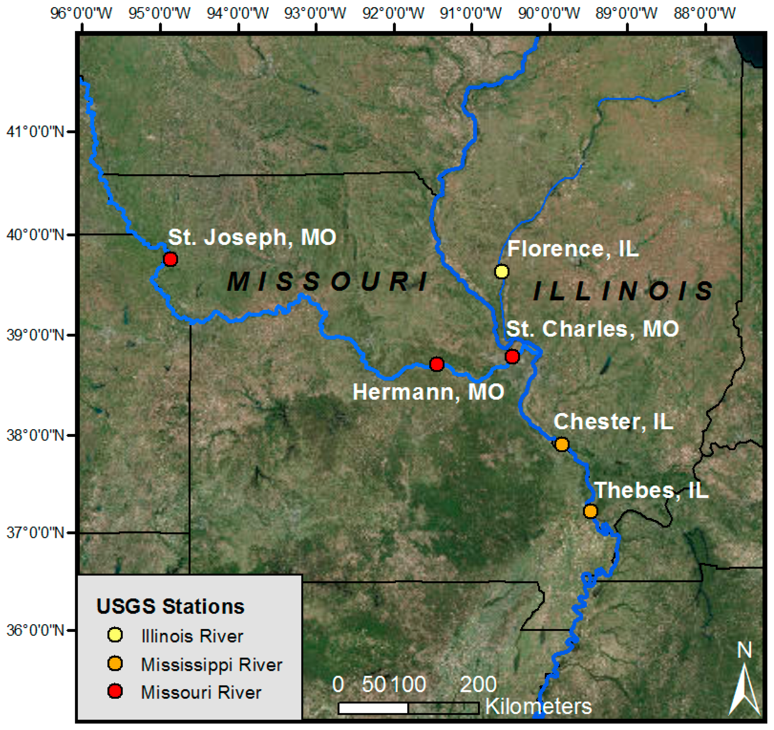
2.1. Study Area

This study focused on modeling SSC across stretches of the lower Missouri and middle Mississippi Rivers. The Missouri–Mississippi River basin encompasses approximately 3,220,000 km2 and is over 5970 km in length, making it one of the largest river systems in the world. Over the past 150 years, both the Missouri and Mississippi Rivers have been subjected to extensive anthropogenic modifications to increase flood control and commercial navigation. These alterations to the natural geomorphology include the construction of dams, channelization, the erection of levees, and impoundments. Modifications such as these, along with resource management changes within the watershed of these rivers, have led to the decline in suspended sediment loads since the 1950s [27].
Due to the importance of understanding localized sediment budgets, significant resources, both state and federal, have been allocated to monitor and quantify trends in SSC within the region. As part of this effort, the United States Geological Survey (USGS) and United States Army Corps of Engineers (USACE) maintain a network of continuous monitoring stations along the Missouri and Mississippi rivers and its major tributaries. To create a predictive reflectance–SSC model, six of these USGS sampling stations were selected (Figure 1). As shown in Figure 1, the sampling locations consisted of three stations along the Missouri River, two along the Mississippi, and one along the Illinois River (a tributary of the Mississippi) to create a range of sampling locations and conditions. The USGS stations used in this study were selected based on the following criteria: (1) SSC must be directly measured and not estimated from turbidity, (2) channel width must be at least 100 m to resolve Landsat 30 m spatial resolution imagery, and (3) the USGS station must contain at least one year of data collection to appropriately represent the site characteristics [15].

2.2. Methods

The methodology for creating a predictive SSC model from Landsat reflectance data is composed of several stages, beginning with the compilation of a pairwise dataset between observed SSC measurements and filtered Landsat imagery. Once the Landsat–SSC database was compiled, a series of spectral band ratios was calculated to create descriptive feature variables to accompany the optical band reflectance values. Using these features and reflectance values, a feature fusion method was applied to eliminate redundant information, improve computational efficiency, and create a single highly informative reflectance variable for regression modeling. The fused spectral information was then used as the input for the regression modeling based on popular ML to produce the final predictive models for SSC.

2.2.1. Suspended Sediment Data

The freely available SSC data were downloaded for the six monitoring stations from the USGS National Water Information System (NWIS) to compile the sediment database. The SSC data provided by the USGS was cross-sectional daily mean SSC reported in milligrams per liter (mg/L), which is computed by the USGS using regression models that relate daily direct point measurements to monthly cross-sectional SSC measurements [28]. An overview of the USGS monitoring stations and their respective data are displayed in Table 1.

2.2.2. Landsat Imagery

The Landsat suite of sensors was chosen for this study due to the free availability of data ranging from 1982 to present and the relatively fine spatial resolution of 30 m conducive to mapping large rivers. Data obtained from all four Landsat sensors were used: Landsat 4 and 5 Thematic Mapper (TM), Landsat 7 Enhanced Thematic Mapper Plus (ETM+), and Landsat 8 Operational Land Imager (OLI). The Landsat sensors also provide relatively fine temporal resolutions with respective 16-day revisit cycles. Utilizing all four Landsat sensors, a wider temporal period can be analyzed and allows for a more continuous monitoring of river systems.
Landsat Level-1 surface-reflectance data products were downloaded from the USGS Earth Explorer website from 1982 to present for the study area to create the Landsat database. To accurately extract filtered and corrected surface-reflectance values at the corresponding USGS sampling locations the image processing routine developed by Pereira et al. [15] was used. First, an atmospheric correction routine was applied to the Level-1 images and the digital number values were then converted to reflectance using image metadata [29,30,31]. Pixels adjacent to each monitoring station were then isolated within a predefined area of interest. Each area of interest for the corresponding sampling sites was defined by a polygon 90 m by 330 m (3 × 11 pixels) to create 33,000 m2 sampling area. The sampling areas were oriented along channel centerlines obtained from the USACE navigational charts which were also used to factor in low-water boundaries. This helped to combat issues related to land adjacency that can lead to errors. The Landsat pixel quality filter was used to ensure only pixels classified as water with low cloud confidence remained. The remaining data contained within the sampling areas were then filtered with a threshold blue band filter of 6.5% for Landsat 4–5 and Landsat 7 and 4.5% for Landsat 8, to filter out effects from cirrus clouds and cloud shadows along with a surface reflectance standard deviation filter of 0.5% to filter out river vessel traffic (Figure 2).
The filtered images in the database were compared to the SSC database to select matching pairs for the regression modeling analysis. Table 2 provides a summary of the corresponding Landsat–SSC database used for modeling. By sensor, this created a database of 425 samples for both Landsat 4–5 and Landsat 7, along with 86 samples for Landsat 8. As displayed in Table 1, the period of record for each selected station varied in length. For example, the Landsat 4–5 database largely consisted of samples from the Chester, IL, Florence, IL, and Thebes, IL locations. Potential bias was confronted by utilizing a random partition of data for modeling and validation.

2.2.3. Suspended Sediment Modeling

The reflectance–SSC modeling utilized the database that contained overlapping non-thermal Landsat surface reflectance and concurrent daily mean SSC values. In addition to the non-thermal reflectance bands, several band ratios [32,33,34,35,36,37] were also created that were previously found useful for satellite-based SSC estimation (Table 3). This created a set of 11 predictor variables for Landsat 4–5 and Landsat 7, and 12 variables for Landsat 8 representing the spectral reflectance characteristics of the given sampling area. The Landsat reflectance information represented the X variables and USGS SSC information the Y variables. Data pertaining to each sensor were randomly partitioned into training (70%) and testing (30%) datasets for the subsequent reflectance–SSC modeling.

2.2.4. Feature Fusion

Feature fusion techniques characteristically take multiple raw input variables or features, such as spectral reflectance values or band ratios and combine them to create a single feature vector which is more informative than any of the individual input features. In this study, a form of canonical correlation analysis (CCA) was employed for feature fusion [38]. This procedure extracts the canonical correlations between two groups of feature vectors to form a unique and more discriminant feature. CCA is a particularly robust method for eliminating redundant information among features and has been found useful in spectroscopic and hyperspectral data analysis [39,40].
The CCA procedure aims to find linear combinations that maximize pair-wise correlations across feature vectors X q x n   and   Y q x n , expressed by
  c o r r ( X * , Y * ) = c o v ( X * , Y * ) v a r ( X * ) . v a r ( Y * ) .  
Let Sxx and Syy denote the intra-set covariance matrices of X (WTx) and Y and Sxy signify the between-set covariance matrix, where cov(X*,Y*) = WTx SxyWy, var(X*) = WTx Sxx Wx and var(Y*) = WTx SyyWy [39]. Maximization is then performed based on the maximum covariance between X* and Y* using var(X*) = var(Y*) = 1 as a constraint. Using principal components analysis (PCA), transformation matrices (Wx and Wy) are created by performing eigenvalue decomposition and by then solving the eigenvalue equations. This generates a diagonal matrix of squares of the canonical correlations [39]. Each non-zero value in the matrix is then sorted by decreasing order to create the final transformation matrices Wx and Wy.
Feature fusion is then performed by summation of the transformed feature matrices
  Z = X * + Y * = W X T X + W Y T Y = ( W x W y ) T ( X Y )  
where T signifies the transformation pair. The resulting Z values are referred to as the canonical correlation discriminant features (CCDFs). The CCA fusion technique was applied to the Landsat reflectance values and band ratios to eliminate redundant spectral information and decrease computational cost. The fused Landsat spectral features were then used as input predictors or explanatory variables in the regression modeling.

2.2.5. Regression Modeling

In this study, several neural network architectures and approaches were explored for estimating SSC from Landsat spectral data and USGS gauge data. Neural networks in their most basic form are structures of fully connected neurons that apply a non-parametric function to the output of a linear regression. These neurons can contain different neural layers or nodes that are interconnected via a weighted linkage. Neural networks are generally defined by three organizational entities: (1) the architecture of interconnection between network nodes, (2) the learning process which automatically updates the weights of the interconnections, and (3) the activation function that converts the networks weighted input with its output [41].
The most widely implemented and common form of neural network modeling is the feedforward neural network (FFNN). The FFNN is a form of supervised learning that passes information forward in the network with no looping, passing first through the input nodes and then through a series of hidden nodes that take in a set of weighted inputs and produce an output through a specified activation function. FFNNs are created by selecting distinct pairs of samples, { x i y i } i = 1 N , from a given training set of N input vectors x i d with the corresponding N output values { y i } i = 1 N . The goal of the model is to determine the relationship between x i and the desired output, y i . Here we implement an FFNN with Bayesian regularization backpropagation containing a single input layer, two hidden layers, and an output layer.
The second neural network approach tested was a cascade-forward neural network (CFNN) that correspondingly utilized Bayesian regularization backpropagation and a similar architecture also containing two hidden layers and the same number of total trainable parameters. CFNNs are like FFNNs but include linkages from each neuron in the input layer and is attached to each neuron in the hidden layer and subsequently all neurons in the output layer. In theory, these additional connections might improve the speed at which the network can learn the desired relationships in the data.
The third regression method tested was extreme learning machine (ELM). A typical ELM is a form of the FFNN that contains an input layer, a single hidden layer, and one output layer. In recent remote sensing studies, ELM has been found to surpass widespread methods such as partial least squares (PLS) and support vector machine (SVM), producing high predictive power while consuming significantly less computational time when dealing with complex spectral interactions [42,43]. ELM gains advantages over other FFNN approaches as the weights of the hidden layer within ELM can be randomly produced and updated without iterative optimization [44]. This in turn leads to significantly less computational time when training the model. The ELM model utilizes the cost function for hidden node L denoted as
  min y i y i ^ i = 1 N = min i = 1 N ( y i j = 1 L β j h j ( w j x i + b j ) )  
where x i is the input, y is the actual output, and y i ^ is the predicted output. ω j d is the weight vector, and b j is the bias of the j hidden node [43], and h ( ) is a nonlinear activation function. The j output weight vector, denoted as βj, is the output weight and links the j hidden node and the output node. For N samples, a compact form for computing β is expressed by
  β =   H T ( 1 λ + H H T ) 1 Y .  
Accordingly, the estimated output value for the i-th input is calculated as
  y ^ i = h ( x i ) T ( I λ + H H T ) 1 Y  
where λ is a user-defined constant, H   refers to the hidden-layer output matrix, Y is the desired output matrix, and I is an identity matrix. An in-depth description of the ELM method is found in [44].
The neural network modeling techniques were selected due to the recent trend in neural network applications in remote sensing and their robust ability to approximate a range of linear and nonlinear functions. To evaluate the effectiveness of the neural network-based approaches, two popular ML methods for remote sensing were used for comparison: SVM [45] and RF [46]. For SVM, sequential minimal optimization [45,47] was utilized to solve the quadratic programming in conjunction with a linear kernel version of the SVM model. The RF model utilized mean square error for the pruning criterion with a minimum leaf size of four, generating an RF model consisting of 99 nodes.
All modeling techniques and procedures were implemented in MATLAB R2018. Apart from ELM, all modeling techniques can be attained from the MATLAB standard library. ELM for regression can be downloaded at http://www.ntu.edu.sg/home/egbhuang/elm_codes.html.

2.2.6. Quantitative Evaluation

To quantitatively analyze the results of the regression modeling process, the coefficient of determination (R2) and the root mean square error (RMSE) were employed. The R2 correlation coefficient represents the proportion of variation in the responses that is explained by the original model using predicted values from the testing dataset. This indicates overall accuracy of the model with higher R2 values representing a higher overall correlation of the model. The RMSE statistic was used to evaluate model error and is calculated as
  R M S E = Σ i = 1 S ( y ˇ i y i ) 2 S  
where y i and y ^ i are the observed and the predicted values and S is the total number of testing samples. Smaller RMSE values indicate a higher overall accuracy and lower predicted error of the model.

3. Results

3.1. Suspended Sediment Modeling

Regression modeling results are displayed in Table 4. ELM generated the highest R2 and lowest RMSE values in all cases when applied to the testing data. Compared to RF and SVM, the ELM model performed slightly better in terms of R2 but displayed significantly lower RMSE. Results for the FFNN and CFNN also displayed significant R2 correlations but produced much higher RMSE values than RF, SVM, and ELM. The ELM model explained over 90% of the SSC data across all Landsat sensors proving to be a robust method for SSC estimation. When applied to the testing datasets, ELM generated an average R2 of 0.916 across Landsat sensors, showing an increase of 4.09%, 7.13%, 9.31%, and 15.51% when compared to SVM, RF, the CFNN, and the FFNN, respectively. The lowest RMSE value was also demonstrated by ELM models with an average testing RMSE across sensors of 45.5, as SVM, RF, FFNN, and CFNN generated RMSE values of 52.2, 57.5, 84.5, and 84.9, respectively. This represents a 12.97% decrease in RMSE values when using ELM compared to SVM that generated the second lowest RMSE.
ELM also displayed negligible overfitting as there was only a minor variance between the training and testing datasets. This is especially notable when applied to the Landsat 8 dataset that only contained 60 samples for training and 26 samples for testing. The FFNN and CFNN methods exhibited higher overfitting compared to RF, SVM, and ELM. As shown in Figure 3, ELM more accurately predicted both high and low values of SSC when compared to the other modeling approaches. The results also displayed that the RF model along with the FFNN and the CFNN appeared to lose accuracy when estimating higher concentrations of SSC. Such decreased accuracy in higher SSC conditions was not demonstrated in either the ELM or SVM model results.
By sensor, the lowest overall results were generated from Landsat 4–5 data with an average R2 of 0.842 and RMSE of 66.6 between modeling techniques. Landsat 7 and Landsat 8 generated higher results with an average R2 of 0.849 and 0.877, respectively. Although Landsat 7 and Landsat 8 displayed similar correlation coefficients, Landsat 8 models resulted in much lower RMSE values with an average of 55.9 compared to the Landsat 7 average RMSE of 72.3.

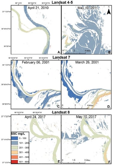
3.2. Suspended Sediment Mapping

To qualitatively evaluate the results of the reflectance–SSC models and filtering process, Landsat images from significant SSC and/or flooding events (Table 5) were selected to illustrate application of the models to a range of hydrologic and SSC conditions. Test cases for each Landsat sensor were evaluated to highlight the fine spatial resolution that can be obtained for SSC estimations. For the first test case, Landsat 4–5 imagery was selected both before and during the 2011 Mississippi River flooding event that lasted from 4 May to 20 June 2011. To represent the normal river conditions, the 21 April 2010 image was selected while the 10 May 2011 image captures the initial stages of the flooding event near Cairo, IL, where significant flooding occurred [48]. The second case utilized Landsat 7 images along the Mississippi River, north of St. Louis, MO, based on a significant rain event that occurred in March of 2001. The 6 February 2001 image represents conditions before the influx of rain, and the 26 March 2001 image displays the results of heavy rains throughout the river basin. The third test case was the May 2017 flooding that occurred along the Missouri and Mississippi Rivers and placed over 10 million residents under flood warnings [49]. Imagery was selected for 24 April 2017 before the flood event and 10 May 2017 after water levels had risen significantly for the area surrounding Cape Girardeau, MO, as the area experienced substantial flooding.
ELM models for each Landsat sensor were tested to illustrate the application of the developed methods for estimating SSC concentrations and monitoring spatial and temporal trends in large fluvial systems. The results of the SSC maps are displayed in Figure 4. As exhibited in Figure 4, the fine spatial resolution of the predicted SSC values provides crucial, continuous information at a localized scale not available from in situ monitoring devices. Given the 30 m spatial resolution of the Landsat imagery, highly detailed SSC patterns are made apparent, especially near confluences such as the confluence of the Ohio and Mississippi Rivers (Figure 4A,B) and the Missouri and Mississippi Rivers (Figure 4C,D). The maps produced in Figure 4 also display the ability to capture temporal changes in SSC that influence local hydrology and sediment budgets. This method represents an efficient and accurate means of producing SSC estimates across vast expanses of large river systems while still maintaining high spatial detail. When compared to the reported daily mean discharge levels in Table 5, the generated SSC maps follow a somewhat linear trend (i.e., as discharge increase so does SSC). Although this is generally true, scenes such as Figure 4B show that, with the applied SSC estimation method, a much more informative data product that contains specific spatial information can be generated. These maps provide a highly improved insight into the SSC dynamics of the waterbody over point based measurements.

4. Discussion

The increased availability and overall quality of satellite-based remote sensing data over the last several decades have greatly improved the ability to remotely monitor inland water bodies without labor and time-intensive in situ sampling. Utilizing data from USGS monitoring stations and the Landsat series of satellites, highly accurate SSC models were generated using the ELM method. In comparison to similar studies such as Pereira et al. [15], the results produced by ELM showed significant improvement generating SSC models for all Landsat sensors with R2 > 0.9 compared to the highest testing result of R2 = 0.78 based on stepwise regression. The developed ELM method also outperformed other similar studies including Umar et al. [21] that generated reflectance–SSC models for Landsat 4–5 with R2 = 0.72 using the RF method. The RF model developed in this study generated improved results with an R2 of 0.853 for Landsat 4–5. Along with exceeding previous findings in terms of R2, the ELM method also displayed a significant reduction in RMSE with an average of 45.4 across sensors compared to 136.0 generated by Pereira et al. [15] and 115.0 by Umar et al. [21]. This improvement can likely be credited to the CCA feature fusion applied to the spectral data which eliminates redundant spectral information and creates highly informative predictor variables. Along with exceeding other reflectance–SSC models, the developed method also outperformed other surrogate methods for SSC quantification such as the acoustic Doppler current profiler method that has a proven accuracy of approximately R2 = 0.8 [50,51].
Findings from several previous studies found that models that performed well at low SSC levels tended to saturate predicted values in cases of higher SSC conditions [11,52]. Due to this issue, several studies propose the use of a switching algorithm depending on the levels of sediment concentrations to improve the model performance [53,54]. In this study, a universal SSC algorithm was utilized with a range of SSC levels up to 750 mg/L. This previously observed phenomenon was demonstrated clearly in the modeling results for RF and slightly in the FFNN and CFNN models (Figure 3). Using the ELM method both low and high values of SSC were accurately predicted (Figure 3) from the Landsat spectral data, although the dataset contained only a small fraction of high SSC values. A potential benefit of the ELM-based method is that all spectral bands and any number of band ratios can be utilized in the model which may also lead to better generalization. ELM has shown promising performance compared to shallow neural networks and traditional remote sensing models in terms of computational efficiency and generalization [44].
The results of ELM’s generalization ability are displayed through the absence of overfitting between the training and testing datasets. When compared to the other modeling approaches tested, ELM showed minimal correlative decay between training and testing accuracies with a mean decrease in R2 of 1.6% compared to 2.6%, 8.2%, 9.5%, and 6.6% for SVM, RF, FFNN, and CFNN, respectively. This in theory allows the ELM-based method to be applied to a wider range of real-world situations such as high or low sediment loads and potentially limit the impact of other variables such as chlorophyll levels on SSC estimation, which can drastically alter the spectral response of the water body [55]. This study supports the trending idea that ML- and neural network-based modeling approaches can significantly improve overall predictive accuracies for complex spectral relationships and interactions, although the still relatively expensive computational requirements could affect the implementation of these techniques. With the use of techniques such as ELM and the USGS monitoring station data, highly accurate reflectance–SSC models can be developed and deployed across the entire Missouri–Mississippi River system to provide monitoring of SSC levels at weekly intervals and continuous spatial extent when based on Landsat data.
The developed models used to predict SSC levels were trained using the mean spectral reflectance values of water pixels adjacent to USGS gauging stations where SSC data were available. The cross-sectional daily mean SSC observations for a given location are collected and derived beneath the water surface in contrast to the Landsat data that largely represents the surface spectral characteristics. Effects such as sun glint and surface waves increase the local variation in water-leaving radiance, but these effects are mitigated through spatial averaging of the Landsat pixels. Other sources of error may also be introduced since satellite information is rarely collected at the exact time of day as the individual SSC measurements. High correlations and relatively low RMSE values generated from the ELM models of predicted SSC suggest that none of these potential sources for error represent inhibiting factors for accurate prediction of a range of SSC levels from Landsat imagery.
Although the proposed methods and resulting reflectance–SSC model was highly predictive there is still a notable and significant limitation in the temporal resolution of Landsat based models representing one of the greatest challenges for remote sensing of SSC. Given Landsat 7 and 8’s revisit cycle of 16 days, the satellite platforms produce imagery over a given area on a weekly basis. For the database generated in this study over half (56%) of the images were eliminated during the filtering process with 31% removed due to cloud cover and 13% due to vessel traffic. This equates to sampling once a month per sensor and represents the limiting factor, as USGS monitoring stations provide daily samples. This dilemma can be improved by utilizing more satellites but still does not address issues related to cloud coverage and vessel traffic.
The application of the developed method to three test cases demonstrates that the technique is effective for quantifying and visualizing temporal and spatial trends in SSC levels within large fluvial systems. The detailed results also showcase the ability of the Landsat suite of sensors to assess local sediment transport and sediment mixing. This technique has the potential to be applied to smaller rivers and streams if based on the finer spatial resolution of the Sentinel satellite suite that contains higher spatial resolution (10 m and 20 m) and twelve bands (Sentinel-2) versus Landsat 8’s eight bands. Models based on Sentinel-2 data could potentially generate higher overall accuracies given an increased number of bands contained within the green, red, and near-infrared regions which are useful for determining SSC.

5. Conclusions

Leveraging widely available and free Landsat data in conjunction with USGS monitoring station data, reflectance–SSC models were developed for the lower Missouri and middle Mississippi River system. The results of the SSC modeling showed that ELM outperformed both FFNN and CFNN, as well as the popular ML techniques such as RF and SVM by significant margins when evaluated by R2 and RMSE. ELM models for all Landsat sensors generated R2 values above 0.9 and displayed noteworthy generalization abilities along with negligible overfitting. ELM proved to be a robust model to predict a wide range of SSC based on a single algorithm. These findings were found to be superior to previous reflectance-SSC models created for the Missouri and Mississippi River systems utilizing more traditional regression techniques such as stepwise regression and RF [15,21].
Utilizing the developed ELM model, SSC maps were generated for the Landsat 4–5, 7, and 8 sensors. Compared to traditional in situ modeling techniques the SSC maps provide continuous spatial coverage which can be used to observe and monitor localized sediment budgets and trends. Applying the ELM-based modeling technique to Landsat 4–5, 7, and 8 allows for long-term temporal monitoring of the Missouri–Mississippi River system ranging from 1982 to the present. Exploring the long-term changes and dynamics in SSC along the river system should be further explored using ELM or other ML techniques as it would establish historical trends at high spatial resolution and accuracy.
Future research should focus on applying ELM or similar modeling techniques to the entire length of the Missouri–Mississippi system. Developments in sensor technology such as improvements in spatial and spectral resolution will further enhance efforts to model SSC in smaller fluvial environments and will enhance the overall knowledge of sediment transport. Future refinements will work to apply the developed method to these newer sensors such as Sentinel-2 that would enable finer resolution SSC estimates. The results of this study demonstrate that ML techniques such as ELM can produce highly accurate reflectance–SSC models that can provide decision makers with valuable sediment information at continuous and finer spatial resolution than those of traditional monitoring methods.

Author Contributions

The paper was conceptualized by K.T.P., V.S., P.S., and A.C. Methodology was formulated by K.T.P., V.S., P.S., and A.C. Landsat 4–5, 7, and 8 imagery along with USGS sediment data were processed by M.M. This study utilized MATLAB R2018 for all modeling and ESRI ArcGIS 10.4 and Harris’s ENVI for image preprocessing.

Funding

Funding for this work were provided in part by the USGS Grant (Award Number: G16AP00066) awarded through the Missouri Water Resources Research Center and The Nature Conservancy (Award Number: 061716-01).

Acknowledgments

A special thanks to Saint Louis University and all who were involved in the research. The authors would also like to extend thanks to the reviewers and editor for their thoughtful review and constructive comments.

Conflicts of Interest

The authors declare no conflict of interest. The funders had no role in the design of the study; in the collection, analyses, or interpretation of data; in the writing of the manuscript; or in the decision to publish the results.

References

  1. Asselman, N.E. Suspended sediment dynamics in a large drainage basin: The River Rhine. Hydrol. Process. 1999, 13, 1437–1450. [Google Scholar] [CrossRef]
  2. Chapra, S.C. Surface Water Quality Modeling. Available online: https://bit.ly/2xcz9Iz (accessed on 17 September 2018).
  3. Welch, H.L.; Coupe, R.H.; Aulenbach, B.T. Concentrations and Transport of Suspended Sediment, Nutrients, and Pesticides in the Lower Mississippi-Atchafalaya River Subbasin during the 2011 Mississippi River Flood, April through July. Available online: https://pubs.er.usgs.gov/publication/sir20145100 (accessed on 17 September 2018).
  4. Kondolf, G.M.; Rubin, Z.K.; Minear, J.T. Dams on the mekong: Cumulative sediment starvation. Water Resour. Res. 2014, 50, 5158–5169. [Google Scholar] [CrossRef]
  5. Meade, R.H.; Moody, J.A. Causes for the decline of suspened-sediment discharge in the Mississippi River system, 1950–2007. Hydrol. Process. 2010, 24, 35–49. [Google Scholar]
  6. Edwards, T.K.; Glysson, G.D. Field Methods for Measurement of Fluvial Sediment. Available online: https://pubs.er.usgs.gov/publication/ofr86531 (accessed on 17 September 2018).
  7. Meade, R.H. Setting: Geology, Hydrology, Sediments, and Engineering of the Mississippi River. Available online: https://pubs.usgs.gov/circ/circ1133/geosetting.html (accessed on 17 September 2018).
  8. Ritchie, J.C.; Schiebe, F.R.; McHenry, J.R. Remote sensing of suspended sediment in surface water. Photogramm. Eng. Remote Sens. 1976, 42, 1539–1545. [Google Scholar]
  9. Feng, L.; Hu, C.; Chen, X.; Tian, L.; Chen, L. Human induced turbidity changes in Poyang Lake between 2000 and 2010: Observations from MODIS. J. Geophys. Res. 2012, 117, 1–19. [Google Scholar] [CrossRef]
  10. Petus, C.; Chust, G.; Gohin, F.; Doxaran, D.; Froidefond, J.M.; Sagarminaga, Y. Estimating turbidity and total suspended matter in the Adour riverplume (south bay of biscay) using MODIS 250-m imagery. Cont. Shelf Res. 2010, 30, 379–392. [Google Scholar] [CrossRef]
  11. Ritchie, J.C.; Zimba, P.V.; Everitt, J.H. Remote sensing techniques to assess water quality. Photogramm. Eng. Remote Sens. 2003, 69, 695–704. [Google Scholar] [CrossRef]
  12. Shen, F.; Verhoef, W.; Zhou, Y.; Salama, M.S.; Liu, X. Satellite estimates of wide-range suspended sediment concentrations in Changjiang (Yangtze) Estuary using MERIS data. Estuaries Coasts 2010, 33, 1420–1429. [Google Scholar] [CrossRef]
  13. Son, S.; Wang, M. Water properties in Chesapeake Bay from MODIS-Aqua measurements. Remote Sens. Environ. 2012, 123, 163–174. [Google Scholar] [CrossRef]
  14. Montanher, O.C.; Novo, E.M.L.M.; Barbosa, C.C.F.; Renno, C.D.; Silva, T.S. Empirical models for estimating the suspended sediment concentration in Amazonian white water rivers using Landsat 5/TM. Int. J. Appl. Earth Obs. Geoinf. 2014, 29, 66–77. [Google Scholar] [CrossRef]
  15. Pereira, L.S.F.; Andes, L.C.; Cox, A.L.; Ghulam, A. Measuring suspended-sediment concentration and turbidity in the middle Mississippi and lower Missouri Rivers using Landsat data. J. Am. Water Resour. Assoc. 2018, 54, 440–450. [Google Scholar] [CrossRef]
  16. Wang, J.J.; Lu, X.X.; Liew, S.C.; Zhou, Y. Retrieval of suspended sediment concentrations in large turbid rivers using Landsat ETM+: An example from the Yangtze River, China. Earth Surf. Process. Landf. 2009, 34, 1082–1092. [Google Scholar] [CrossRef]
  17. Wu, G.; Cui, L.; Liu, L.; Chen, F.; Fei, T.; Liu, Y. Statistical model development and estimation of suspended particulate matter concentrations with Landsat 8 OLI images of Dongting Lake, China. Int. J. Remote Sens. 2015, 36, 343–360. [Google Scholar] [CrossRef]
  18. Zhang, M.; Dong, Q.; Cui, T.; Xue, C.; Zhang, S. Suspended sediment monitoring and assessment for Yellow River Estuary from Landsat TM and ETM+ imagery. Remote Sens. Environ. 2014, 146, 136–147. [Google Scholar] [CrossRef]
  19. Zheng, Z.; Li, Y.; Guo, Y.; Xu, Y.; Liu, G.; Du, C. Landsat-based long-term monitoring of total suspended matter concentration pattern change in the wet season for Dongting Lake, China. Remote Sens. 2015, 7, 13975–13999. [Google Scholar] [CrossRef]
  20. Bukata, R.P.; Jerome, J.H.; Kondratyev, A.S.; Pozdnyakov, D.V. Optical Properties and Remote Sensing of Inland and Coastal Waters. Available online: https://bit.ly/2OsMMd3 (accessed on 17 September 2018).
  21. Umar, M.; Rhoads, B.L.; Greenburg, J.A. Use of multispectral satellite remote sensing to assess mixing of suspended sediment downstream of large river confluences. J. Hydrol. 2018, 556, 325–338. [Google Scholar] [CrossRef]
  22. Zhang, Y.Z.; Pullianen, J.T.; Koponen, S.S.; Hallikainen, M.T. Application of an empirical neural network to surface water quality estimation in the Gulf of Finland using combined optical data and microwave data. Remote Sens. Environ. 2002, 81, 327–336. [Google Scholar] [CrossRef]
  23. Hassoun, M.H. Fundamentals of Artificial Neural Networks. Available online: https://amzn.to/2Ni38IV (accessed on 17 September 2018).
  24. Sudheer, K.P.; Chaubey, I.; Garg, V. Lake water quality assessment from Landsat thematic mapper data using neural network: An approach to optimal band combination selection. J. Am. Water Resour. Assoc. 2006, 42, 1683–1695. [Google Scholar] [CrossRef]
  25. Mas, J.F.; Flores, J.J. The application of artificial neural networks to the analysis of remotely sensed data. Int. J. Remote Sens. 2008, 29, 617–663. [Google Scholar] [CrossRef]
  26. Chebud, Y.; Naja, G.M.; Rivero, R.G.; Melesse, A.M. Water quality monitoring using remote sensing and an artificial neural network. Water Air Soil Pollut. 2012, 223, 4875–4887. [Google Scholar] [CrossRef]
  27. Heimann, D.C.; Sprague, L.A.; Blevins, D.W. Trends in Suspended-Sediment Loads and Concentrations in the Mississippi River Basin. Available online: https://pubs.usgs.gov/sir/2011/5200/pdf/sir2011-5200.pdf (accessed on 17 September 2018).
  28. Koltun, G.F.; Eberle, M.; Gray, J.R.; Glysson, G.D. USGS Geological Survey Techniques and Methods. Available online: https://pubs.usgs.gov/tm/tm7c5/pdf/TM-7-C5.pdf (accessed on 17 September 2018).
  29. United States Geological Survey. Landsat Thematic Mapper (TM) Level 1 (L1) Data Format Control Book (DFCB). Available online: https://landsat.usgs.gov/sites/default/files/documents/LSDS-284.pdf (accessed on 17 September 2018).
  30. United States Geological Survey. Landsat 8 (L8) Level 1(L1) Data Format Control Book. Available online: https://bit.ly/2xiVxzV (accessed on 17 September 2018).
  31. United States Geological Survey. Landsat 4-7 Climate Data Record (CDR) Surface Reflectance. Available online: https://on.doi.gov/2xvg5oa (accessed on 17 September 2018).
  32. Dekker, A.G.; Vos, R.J.; Peters, S.W.M. Analytical algorithms for lake water TSM estimation for retrospective analyses of TM and SPOT sensor data. Int. J. Remote Sens. 2002, 23, 15–35. [Google Scholar] [CrossRef]
  33. Doxoran, D.; Froidefond, J.M.; Castaing, P. Remote-sensing reflectance of turbid sediment-dominated waters reduction of sediment type variations and changing illumination conditions effects by use of reflectance ratios. Appl. Opt. 2003, 42, 2623–2634. [Google Scholar] [CrossRef]
  34. Joshi, I.D.; D’Sa, E.J.; Osborn, C.L.; Bianchi, T.S. Turbidity in Apalachicola Bay, Florida from Landsat 5 TM and field data: Seasonal patterns and response to extreme events. Remote Sens. 2017, 9, 367. [Google Scholar] [CrossRef]
  35. Lathrop, R.G.; Lillesand, T.M. Monitoring water-quality and river plume transport in Green Bay, Lake-Michigan with SPOT-1 imagery. Photogramm. Eng. Remote Sens. 1989, 55, 349–354. [Google Scholar]
  36. Onderka, M.; Pekárová, P. Retrieval of suspended particulate matter concentrations in the Danube River from Landsat ETM data. Sci. Total Environ. 2008, 397, 238–243. [Google Scholar] [CrossRef] [PubMed]
  37. Svab, E.; Tyler, A.N.; Preston, T.; Presing, M.; Balogh, K.V. Characterizing the spectral reflectance of algae in lake waters with high suspended sediment concentrations. Int. J. Remote Sens. 2005, 26, 919–928. [Google Scholar] [CrossRef]
  38. Sun, Q.S.; Zeng, S.G.; Liu, Y.; Heng, P.A.; Xia, D.S. A new method of feature fusion and its application in image recognition. Pattern Recognit. 2005, 38, 2437–2448. [Google Scholar] [CrossRef]
  39. Haghighat, M.; Abdel-Mottaleb, M.; Alhalabi, W. Fully automatic face normalization and single sample face recognition in unconstrained environments. Expert Syst. Appl. 2015, 47, 23–34. [Google Scholar] [CrossRef]
  40. Peterson, K.T. Machine Learning Based Ensemble Prediction of Water Quality Variables Using Feature-Level and Decision-Level Fusion; Remote Sensing Saint Louis University: St. Louis, MO, USA, 2018. [Google Scholar]
  41. Verrelst, J.; Camps-Valls, G.; Muñoz-Marí, J.; Rivera, J.P.; Veroustraete, F.; Clevers, J.G.; Moreno, J. Optical remote sensing and the retrieval of terrestrial vegetation bio-geophysical properties—A review. ISPRS J. Photogramm. Remote Sens. 2015, 108, 273–290. [Google Scholar] [CrossRef]
  42. Lin, Y.; Yu, J.; Cai, J.; Sneeuw, N.; Li, F. Spatio-temporal analysis of wetland changes using a kernel extreme learning machine approach. Remote Sens. 2018, 10, 1129. [Google Scholar] [CrossRef]
  43. Maimaitijiang, M.; Ghulam, A.; Sidike, P.; Hartling, S.; Maimaitiyiming, M.; Peterson, K.T.; Shavers, E.; Fishman, J.; Peterson, J.; Kadam, S.; et al. Unmanned aerial system (UAS)-based phenotyping of soybean using multi-sensor data fusion and extreme learning machine. ISPRS J. Photogramm. Remote Sens. 2017, 134, 43–58. [Google Scholar] [CrossRef]
  44. Huang, G.B.; Zhu, Q.Y.; Siew, C.K. Extreme learning machine: Theory and 641 applications. Neurocomputing 2006, 70, 489–501. [Google Scholar] [CrossRef]
  45. Schölkopf, B.; Smola, A.J. Learning with Kernels: Support Vector Machines, Regularization, Optimization, and Beyond. Available online: https://dl.acm.org/citation.cfm?id=559923 (accessed on 17 September 2018).
  46. Liaw, A.; Wiener, M. Classification and regression by randomforest. R News 2002, 2, 18–22. [Google Scholar]
  47. Fan, R.E.; Chen, P.H.; Lin, C.J. Working set selection using second order information for training support vector machines. J. Mach. Learn. Res. 2005, 6, 1889–1918. [Google Scholar]
  48. Alexander, J.S.; Jacobson, R.B.; Rus, D.L. Sediment Transport and Deposition in the Lower Missouri River during the 2011 Flood. Available online: https://pubs.usgs.gov/pp/1798f/ (accessed on 17 September 2018).
  49. Heimann, D.C.; Holmes, R.R.J.; Harris, T.E. Flooding in the Southern Midwestern United States, April–May 2017: U.S. Geological Survey Open-File Report. Available online: https://bit.ly/2OrL5g5 (accessed on 17 September 2018).
  50. Gray, J.R.; Gartner, J.W. Technological advances in suspended-sediment surrograte monitoring. Water Resour. Res. 2009, 45. [Google Scholar] [CrossRef]
  51. Wall, G.R.; Nystrom, E.; Litten, S. Use of ADCP to Compute Suspended Sediment Discharge in the Tidal Hudson River, NY. Available online: https://bit.ly/2OtSgV5 (accessed on 17 September 2018).
  52. Long, C.M.; Pavelsky, T.M. Remote sensing of suspended sediment concentration and hydrologic connectivity in a complex wetland environment. Remote Sens. Environ. 2013, 129, 197–209. [Google Scholar] [CrossRef]
  53. Feng, L.; Hu, C.; Chen, X.; Song, Q. Influence of the Three Gorges Dam on total suspended matters in the Yangtze Estuary and its adjacent coastal waters: Observations from MODIS. Remote Sens. Environ. 2014, 140, 779–788. [Google Scholar] [CrossRef]
  54. Han, B.; Loisel, H.; Vantrepotte, V.; Mériaux, X.; Bryère, P.; Ouillon, S.; Dessailly, D.; Xing, Q.; Zhu, J. Development of a semi-analytical algorithm for the retrieval of suspended particulate matter from remote sensing over clear to very turbid waters. Remote Sens. 2016, 8, 211. [Google Scholar] [CrossRef]
  55. Jensen, J.R. Remote Sensing of the Environment: An Earth Resource Perspective (Second Edition). Available online: https://amzn.to/2OrZx7W (accessed on 17 September 2018).
Figure 1. Map of the study area detailing the six United States Geological Survey (USGS) sampling stations color coded by the major rivers they are located along.
Remotesensing 10 01503 g001
Figure 2. Examples of the Landsat image filtering process near the confluence of the Missouri and Mississippi rivers. The top panel displays the level-1 surface reflectance for each Landsat sensor and the bottom panel the resulting surface reflectance after the filtering process. All images are visualized in RGB bands.
Remotesensing 10 01503 g002
Figure 3. Plots of the observed versus predicted SSC values when applied to the testing dataset. Plots are arranged by sensor and modeling technique with R2 values representing the overall fit of the model.
Remotesensing 10 01503 g003
Figure 4. Maps of predicted SSC based on the ELM model for the three test cases. Panel A displays Landsat 4–5 SSC predictions for 21 April 2010, and Panel B shows the SSC predictions for 10 May 2011 for the area surrounding Cairo, IL. Panels C and D represent the SSC conditions pre- and post-rain events in 2001 based on Landsat 7 data North of St. Louis, MO. Panels E and F display the SSC conditions near Cape Girardeau, MO both pre-and post the 2017 flood event. Blue represents lower SSC while red represents higher levels of SSC.
Remotesensing 10 01503 g004aRemotesensing 10 01503 g004b
Table 1. Site descriptions of all available USGS suspended sediment monitoring stations within the study area.
USGS Station IDStation NamePeriod of RecordDrainage Area (km2)
07020500Chester, IL1 October 1982–30 September 20171,140,381.16
05586300Florence, IL13 February 1980–29 September 201443,243.07
06934500Hermann, MO24 February 2006–11 March 201843,243.07
06935965St. Charles, MO1 October 2005–30 September 2008843,296.26
06818000St. Joseph, MO1 March 2006–2 April 2018686,385.22
07022000Thebes, IL1 October 1982–30 September 20171,147,784.14
Table 2. Statistics of the filtered suspended sediment concentration (SSC) data corresponding to Landsat imagery.
USGS Station IDStation NamePeriod of RecordSamples (n)SSC mg/L
MinMaxMean
07020500Chester, IL12 January 1983–20 September 201618739.0863.0236.1
05586300Florence, IL3 January 1983–22 September 201426617.8860.0140.7
06934500Hermann, MO8 March 2009–12 July 20178246.81200.0288.0
06935965St. Charles, MO15 October 2005–12 August 200827116.0667.0233.7
06818000St. Joseph, MO4 October 2008–25 July 201786150.01100.0359.4
07022000Thebes, IL3 September 1984–20 September 201628840.9961.0218.8
Table 3. Spectral band ratios for suspended sediment retrieval from multispectral satellite sensors. The R2 value represents the linear correlation between the ratio and the measured SSC for each sensor.
Band RatioR2
Landsat 4–5Landsat 7Landsat 8
(Green + Red)/20.2970.3450.401
Green/Red0.4740.4550.478
Red/Green0.5130.5030.552
NIR/Green0.4450.4480.640
Red/Green + NIR0.4840.5050.720
Red0.4130.3490.497
NIR0.4590.4070.714
Table 4. Results of the regression modeling between the Landsat spectral information and measured SSC. Highlighted in bold are the best results for each sensor when applied to testing data.
Regression Model Results
Landsat 4–5Landsat 7Landsat 8
TrainingTestingTrainingTestingTrainingTesting
R2RMSER2RMSER2RMSER2RMSER2RMSER2RMSE
RF0.94237.60.85356.70.94241.20.86057.60.91157.00.85258.0
SVM0.85658.20.82759.50.89052.60.88456.80.96237.10.92840.4
FFNN0.85575.40.78288.80.86882.10.81493.10.90971.60.78371.7
CFNN0.85581.10.83682.70.90373.50.786102.30.93368.90.89169.7
ELM0.91643.30.91445.20.91048.10.90351.40.96834.20.93139.7
Table 5. Date and location information for the selected images used to generate SSC maps. Dates were chosen to highlight significant SSC events along the Missouri–Mississippi River system. Discharge levels represent the mean daily discharge and are reported using the nearest USGS monitoring location with available data.
SensorLocationImage DateDischarge (m3)USGS Station Location
Landsat 4–5Mississippi River near Cairo, IL21 April 201010,279Mississippi River at Thebes, IL
10 May 201116,225
Landsat 7Mississippi River, North of St. Louis, MO6 February 20012673Mississippi River at Grafton, IL
26 March 20016456
Landsat 8Mississippi River near Cape Girardeau, MO24 April 201710,364Mississippi River at Thebes, IL
10 May 201721,776

