Article

Assessment of Scattering Error Correction Techniques for AC-S Meter in a Tropical Eutrophic Reservoir

1
Department of Cartography, Faculty of Science and Technology, UNESP—Universidade Estadual Paulista, Rua Roberto Simonsen 305, Presidente Prudente, SP 19060-900, Brazil
2
Federal Institute of Education, Science and Technology from Pará, Rodovia BR 316, km 61, Castanhal, PA 68740-970, Brazil
3
Department of Environmental Engineering, Institute of Science and Technology, UNESP—Universidade Estadual Paulista, Rodovia Presidente Dutra km 137.8, São José dos Campos, SP 12247-004, Brazil
4
Department of Mathematics and Computer Science, Faculty of Science and Technology, UNESP—Universidade Estadual Paulista, Rua Roberto Simonsen 305, Presidente Prudente, SP 19060-900, Brazil
*
Author to whom correspondence should be addressed.
Remote Sens. 2018, 10(5), 740; https://doi.org/10.3390/rs10050740
Submission received: 13 February 2018 / Revised: 19 April 2018 / Accepted: 20 April 2018 / Published: 11 May 2018

Abstract

:
Measurements of absorption coefficients (a(λ), in m−1) collected by spectrophotometers in situ are overestimated due to the scattering of the reflecting tube absorption meter. Accurate correction of these data is essential in order to characterize water bodies bio-optically, as well as retrieve the remote sensing reflectance (Rrs, in sr−1), when applying a forward model. There are various methods of scattering error correction; however, they were all developed for clear water. In this research, different techniques were attempted in order to define the most appropriate method for correcting a(λ) values acquired by an absorption and attenuation spectral (ac-s) meter (WET Labs Inc., Philomath, OR, USA) in a tropical eutrophic reservoir. Three methods recommended by the manufacturer of the ac-s meter were tested: “flat” or “baseline”, “constant fraction”, and “proportional”. These methods were applied to two datasets that were measured in May and October 2014. The flat technique exhibited the lowest errors, with an average normalized root mean square error (NRMSE) of 7.95%, and a mean absolute percentage error (MAPE) of 29.26% for May. Meanwhile, proportional was the most suitable technique for most of the samples in October, with a mean NRMSE of 11.19% and a MAPE of 31.03% for October. In addition, the proportional method maintained the shape of the a(λ) values better than the other methods. Despite that, both the flat and proportional methods gave a similar performance statistically. Moreover, the flat method produced the best estimations of chla content for both datasets. Therefore, this method is recommended to correct ac-s data in retrieving such phytoplankton pigments.

1. Introduction

Absorption and scattering coefficients (a(λ) and b(λ), respectively) are inherent optical properties (IOPs) of water [1] that enable the bio-optical characterization of aquatic systems and the underwater light climate to be understood due to variations in optically significant constituents (OSCs) [2,3,4,5,6,7,8,9,10,11]. The sum of a(λ) and b(λ) represents the light extinction or attenuation coefficient (c(λ)) in the water column [1]. Such coefficients are important in studies about primary production [12,13,14,15], photosynthesis [12,13], and energy transfer [16].
In addition, a(λ) and b(λ) are directly associated with measurements of remote sensing reflectance (Rrs), as shown in Equation (1) [17], modeling the magnitude and shape of Rrs according to the composition of OSCs and their concentrations [18,19]. Hence, this relationship has been widely used in inverse and forward models to retrieve concentrations of OSCs [20,21,22,23]. For the second one of these, accurate measurements of a(λ) and bb(λ) are necessary in order to prevent error propagation in subsequent steps:
R rs ( λ ) b b ( λ ) b b ( λ ) + a ( λ )
where Rrs is the remote sensing reflectance; bb is the backscattering coefficient; and a is the absorption coefficient.
In this context, measurements of a(λ) and c(λ) were acquired using an absorption and attenuation spectral (ac-s) meter (WET Labs Inc., Philomath, OR, USA); these have been used in many studies. Martinez-Vicente et al. [24] used b(λ) derived by subtracting a(λ) from c(λ) to investigate the spectral behavior and variability of OSCs [24]. Additionally, ac-s data have been used to correct measurements of bb(λ) collected by sensors such as HydroScat-6P (HOBI Labs, Bellevue, WA, USA) and ECO-BB9 (WET Labs Inc., Philomath, OR, USA) [7,25]. These data have been used in research studies about the biogeochemical gradient [10,26,27] and filtration process in cascading reservoir systems [11]. However, a(λ) data acquired by an ac-s meter are often overestimated due to the light scattering of the reflecting tube absorption meter [28].
Some techniques were developed to correct this effect [28,29,30,31]. In the user’s guide, the manufacturer recommends three techniques: “flat” or “baseline” [28], “constant fraction” [29] and “proportional” [28]. The constant fraction technique assumes that the overestimated a(λ) fraction matches a b(λ) fraction measured by equipment that takes into account a rate of b(λ) related to the type of water [29,30]. Meanwhile, the flat and proportional techniques consider a reference wavelength (λ0), where a(λ) should be equal or close to zero [28]. In other words, the assumption is that the a(λ) value reported actually matches b(λ). In the flat method, b(λ) in the absorption tube is considered equal at every wavelength; therefore, a0) is directly subtracted from a(λ), while, in the proportional method, b(λ) is variable.
These methods were originally developed for marine waters and regions of temperate climate [28,29,30,31,32,33]. Overall, open ocean waters exhibit much lower a(λ) than inland waters due to lower primary productivity and sediments coming from the watershed. Roesler [34] reported a maximum a(412) lower than 2 m−1 for oceanic waters, while Carvalho et al. [25] observed a(412) ranging from 8 m−1 to 17 m−1 in the Lago Grande de Curuai (Amazon River), which is a highly turbid water body (turbidity range of 90 NTU to 1645 NTU). Carvalho et al. [25] also evaluated some of these correction methods in order to determine the most appropriate for that sort of environment. They [25] simulated Rrs using a(λ) corrected from different techniques and compared them with Rrs measured in situ to assess the performance of each method.
Suspended matter is predominately composed of inorganic components in the Lago Grande de Curuai, but it is the organic fraction that is dominant in our study area due to high primary production. We therefore posed the follow question: How does an intense algal bloom affect the scattering correction techniques in a reflective tube absorption meter? Hence, the main goal of this research was to attempt three methods of correction in order to determine the most appropriate for eutrophic waters. The specific aims were: (a) to verify how the bio-optical variability affects the scattering in an absorption tube in productive waters; (b) to access whether the use of the 750-nm wavelength can be used to correct a(λ); and (c) to evaluate the influence of correction performance over bio-optical modeling. Measurements of a(λ) and c(λ) were therefore collected using an ac-s meter in the Barra Bonita (BB) reservoir, which has a high primary production. To assess the correction methods, data of a(λ) were measured in the laboratory using a spectrophotometer.

2. Materials and Methods
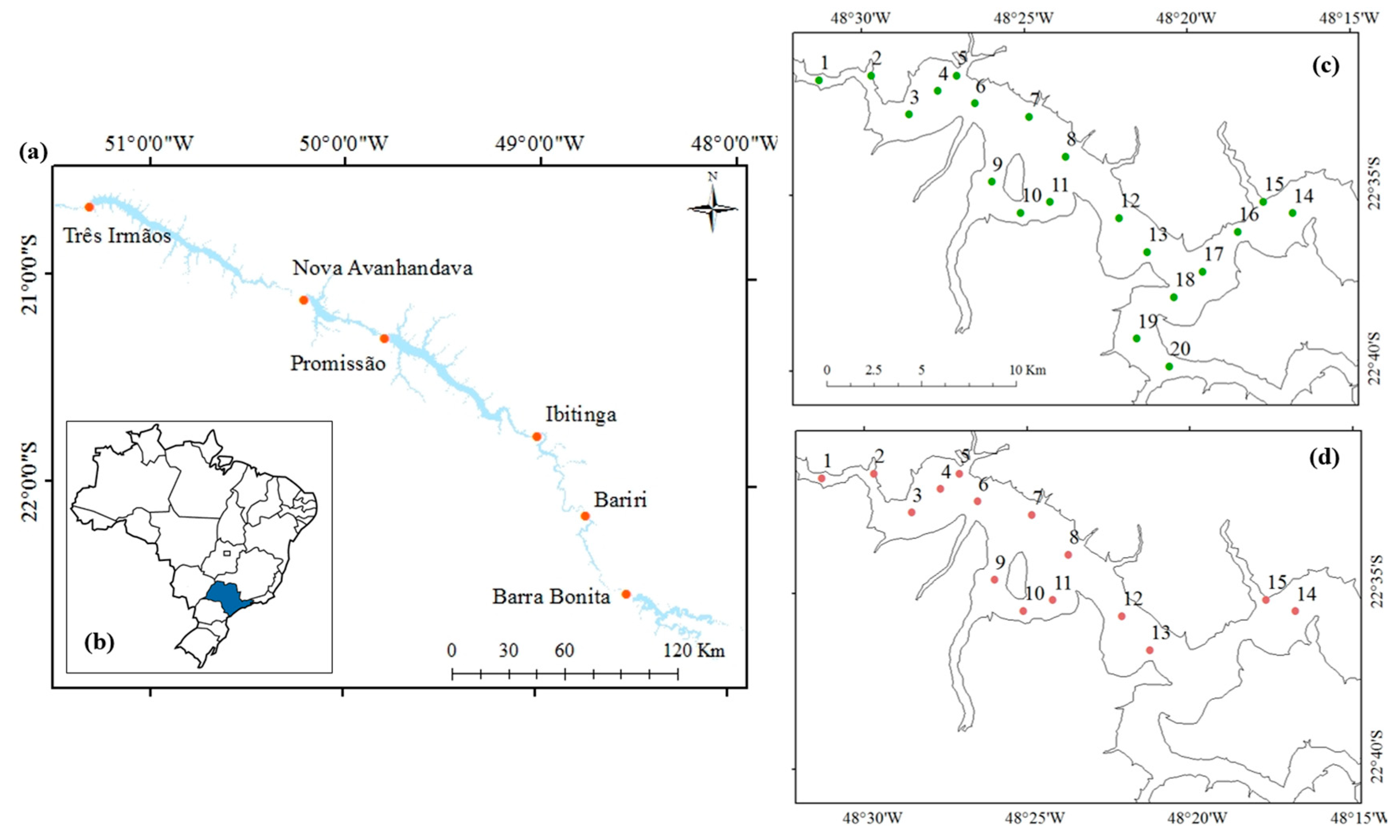
2.1. Study Area

Two datasets were collected in the BB hydroelectric reservoir (22°31′10″S and 48°32′3″W), which lies on the middle course of the Tietê River, São Paulo State, Brazil (Figure 1). BB is the first in a cascading reservoir system on the Tietê River, and therefore receives a high nutrient load coming from the Sao Paulo metropolitan area, which is responsible for its eutrophic status [35,36]. The hydroelectric plant has been in operation since 1963, when the reservoir flooded an area of 310 km2, with a volume of approximately 3.622 × 10⁶ m3 (AES Tietê, www.aestiete.com.br). The average depth is of 10.2 m, with a maximum of 25 m [36], while the water level ranges from 439.5 m to 451.5 m (AES Tietê). The flow rate is approximately 1500 m3 s−1 during the austral summer (wet season from December to March), and 200 m3 s−1 in the austral winter (dry season from June to September), influencing the retention time of 30 days (austral summer) to 180 days (austral winter) [37]. The BB reservoir receives a high nutrient load from the São Paulo metropolitan area, leading to harmful algal blooms. Taking into account the concentration of chlorophyll a (chla), the BB reservoir was classified as hypertrophic and dominated by algal particles [38]. In addition, there is a richness of phytoplankton species [36,37,39], with a predominance of cyanobacteria in the austral summer and diatoms in the austral winter [39]. Cyanobacteria are often associated with the occurrence of the thermal stratification and stability of the water column in BB [40]. According to Barbosa et al. [41], BB is considered a polymictic system, which experiences fluctuations in rainfall, wind, and intrusion of water from tributaries, with a low retention time during the austral summer and density currents due to the contribution of the main tributaries (Tietê and Piracicaba rivers). Such variables affect both the horizontal and vertical mixing processes in the reservoir.

2.2. Data Collection

Two field surveys were carried out between 5–9 May 2014 (austral autumn) and 13–16 October 2014 (austral spring). Low rainfall and medium temperatures characterize the austral autumn, while medium rainfall and high temperatures are observed in the austral spring. Twenty samples were collected in the first campaign, while 15 samples were acquired in the second. Measurements of a(λ) and c(λ) were acquired in situ, using an ac-s meter, with a 10-cm optical path. The equipment works in a spectral range of 400 nm to 742 nm, with a resolution precision of about 4 nm (WET Labs Inc., Philomath, OR, USA). A conductivity, temperature, and depth (CTD) sensor, model 37SI (SEA-BIRD Electronic, Bellevue, WA, USA) was submerged simultaneously with the ac-s meter. Both the ac-s and CTD sensors were coupled to a data handler with four ports (DH-4), which is a sensor interface module that enables the collection, storage, and merging of data from different devices (WET Labs Inc., Philomath, OR, USA). Water samples were also collected just below the surface at each sampling station to determine a(λ) and OSC (chla and suspended matter) concentrations in the laboratory. Turbidity and Secchi disk depth (SDD, in m) were collected at every sampling station.

2.3. Correction of ac-s Data

2.3.1. Temperature and Salinity Correction

The ac-s data were processed using the software wap34 (WET Labs Archive File Processing) (WET Labs Inc., Philomath, OR, USA). This program allows the processing of data files collected by sensors linked to a DH-4. Temperature and salinity effects on pure water absorption (aw) were removed from the ac-s measurements [42]. The correction was carried out using the method proposed by Sullivan et al. [43] from data collected by a CTD sensor as input for corrections. Detailed information about procedures used in this work are presented in Imai et al. [44].

2.3.2. Scattering Error Correction

After correcting for the temperature and salinity effects, the scattering of the reflecting tube was also removed from the ac-s data. The three methods recommended by the manufacturer were tested: flat, proportional [28], and constant fraction [29]. The flat technique consists in subtracting the absorption measured at a reference wavelength, am0), of the absorption measured at every wavelength, am(λ), considering that am0) must be equal to zero, i.e., it is assumed that the OSC absorption (absorption of particles and absorption of colored dissolved organic matter (CDOM), ap + aCDOM) is negligible at λ0 (Equation (2)):
a flat ( λ ) = a m ( λ ) a m ( λ 0 )
where aflat is the absorption corrected by the flat method; am(λ) is the spectral absorption measured by an ac-s meter; and am0) is the absorption measured by an ac-s meter at reference wavelength (λ0). In marine waters, 715 nm is commonly used as λ0 [28]; however, in inland waters, OSC absorption is very high, and therefore, the choice of λ0 is shifted to longer wavelengths [25,32]. In this work, we used the wavelength at 740 nm as λ0, although the temperature strongly affects a(λ) by pure water at around 754 nm [28,43]. However, some studies show that the use of longer wavelengths as λ0 do not produce a negative prediction in inland waters [25].
The proportional method proposed by Zaneveld et al. [28] also considers a λ0 to determine the proportion of b(λ) to subtract from am(λ), as shown in Equation (3). In this method, we also adopted 740 nm as λ0. The b(λ) value used in this formula is derived by subtracting the absorption from the attenuation, which are both measured by an ac-s meter:
a prop ( λ ) = a m ( λ ) a m ( λ 0 ) · b m ( λ ) b m ( λ 0 )
where aprop is the absorption corrected by the proportional method; am(λ) is the absorption measured by an ac-s meter; am0) is the absorption value at λ0; bm(λ) is the scattering estimated by the attenuation minus the absorption measured by an ac-s meter; and bm0) is the scattering calculated from an ac-s meter at λ0.
The constant fraction method proposed by Kirk [29] considers that ‘true’ a0) (acf) is the measured absorption coefficient, am, minus the product of the measured backscattering coefficient, bm, times a constant factor related to a particular phase function, w (Equation (4)). Both am and bm were measured by an ac-s meter:
a cf ( λ ) = a m ( λ ) w · b m ( λ )
Kirk [29] used a Monte Carlo model to describe the behavior of photons in a reflective tube absorption meter, defining the reflectivity of the tube, which is used to determine w. The author found a w of 0.162 for turbid coastal waters and 0.207 for clear marine waters. WET Labs protocol suggests a w of 0.14 for biological particles-dominated scattering, while a w of 0.18 is recommended for sediments-dominated scattering. McKee et al. [30] established a weighting function that describes the collection of angular scattering for an ac-9 reflecting tube absorption meter (WET Labs Inc., Philomath, OR, USA) and also applies Monte Carlo simulations. Although b(λ) is dominated by phytoplankton in the BB reservoir, a value of 0.18 as adopted for w due to high attenuation was found in the study area.

2.4. Absorption Measured in the Laboratory

Measurements of a(λ) determined in the laboratory were adopted as ground true to optical closure. In this work, the a(λ) values of particulate material and colored dissolved organic matter (ap(λ) and aCDOM(λ), respectively) were separately measured to derive a(λ). To determine ap(λ), water samples were filtered through Whatman GF/F glass fiber filters, with a 47-mm diameter and a 0.7-μm pore size (GE Healthcare, Little Chalfont, UK). The filters with material retained were stored in sterile jars, and kept frozen and in the dark until analysis. The reflectance–transmittance method developed by Tassan and Ferrari [45,46,47] was used. Reflectance and transmittance measurements were taken using a UV-Vis spectrophotometer, model UV-2600 (Shimadzu, Kyoto, Japan), dual beam mode, and integration sphere. Data were acquired in a range of 280 nm to 800 nm, with a spectral resolution of 1 nm. A clear filter was used as a blank reference to correct the multiple scattering effects caused by the filter itself [48]. The optical density of the retained particle sample (ODs(λ)) on the filter was derived from the measurements and empirically converted into the optical density of the suspended particles (ODp(λ)), as shown in Tassan and Ferrari [47] (Equation (5)):
O D p ( λ ) = 0.423 · O D S + 0.479 · O D S 2
Finally, ap(λ) was calculated using the relation presented in Equation (6) [45,48]:
a p ( λ ) = 2.3   O D p ( λ ) ( V A )
where ODp(λ) is the optical density of the particles on the filter; V is the filtered volume; and A is the fiber clearance area (m2).
To determine aCDOM, the water samples filtered in the Whatman GF/F glass fiber were refiltered on a Whatman nylon membrane filter (GE Healthcare, Little Chalfont, UK), with a 0.22 pore size and 47-mm diameter. The water filtered twice was stored in sterile jars of 100 ml, and kept cool and in the dark until analysis. Absorbance of CDOM (ACDOM) was measured with the samples at room temperature in a UV-Vis spectrophotometer, model UV-2600 (Shimadzu, Kyoto, Japan), using single beam mode. The samples were inserted into a cuvette with a 10-cm optical path. Also, ultrapure water was used as a blank reference. ACDOM was measured in a spectral range of 280 nm to 800 nm, with a spectral resolution of 1 nm. This data was used to calculate aCDOM from Equation (7) [49]:
a CDOM ( λ ) = 2.3   A CDOM ( λ ) l
where ACDOM is the absorbance of CDOM at wavelength λ, and l is the path length of the cuvette in meters.

2.5. Chla and TSM Concentrations

To estimate chla and total suspended matter (TSM) concentrations, water samples were collected and filtered on a Whatman GF/F glass fiber filter, with a 0.7-μm size pore and a 47-mm diameter. The filters were stored frozen and in the dark until analysis. In May, a volume of 500-mL of water was filtered in each filter, while, in October, just 250 ml of water was filtered due to a higher solid content.
Chla extraction was done using a 90% acetone solution [50]. Measurements of absorbance were acquired at 663 nm and 750 nm, using a FEMTO spectrophotometer (FEMTO, São Paulo, Brazil). After samples were acidified with a 0.1-N HCl solution, new readings of absorbance were done to reduce the influence of phaeophytin (degradation product of chla). Acetone solution was used as a blank reference. TSM concentration was estimated following the APHA method [51]. Before filtering, Whatman GF/F filters were prepared by igniting at 500 °C for 30 min in a muffle furnace, and were then desiccated and weighed to determine the initial filter mass. After filtering, the material retained on the filters was dried in an oven at 105 °C to 110 °C for 12 h. The filters were desiccated and weighed to obtain the TSM mass by subtracting the initial filter mass. The volatile solids were ignited in a muffle furnace at about 500 °C for 30 min. Again, the filters were desiccated and weighed to estimate the inorganic suspended matter (ISM) mass by subtracting the initial filter mass. Consequently, the organic suspended matter (OSM) was determined by subtracting the TSM of the ISM mass. TSM, ISM, and OSM masses were divided by the filtered water sample volume to estimate their respective concentrations.

2.6. Evaluation of the Correction Techniques

The corrected a(λ) values were compared to the a(λ) values that were measured in the laboratory derived from the sum of aCDOM(λ) and ap(λ). Correction methods were evaluated based on statistical metrics: root mean square error (RMSE, Equation (8)), normalized root mean square error (NRMSE, Equation (9)), mean absolute percentage error (MAPE, Equation (10)), and bias (Equation (11)):
R M S E = 1 n i = 1 n ( x i x i ) 2
N R M S E = R M S E x max x min
M A P E = 1 n i = 1 n ( | x i x i x i | )
b i a s = 1 n i = 1 n ( x i x i )
where xi is the absorption spectral measured using an ac-s meter and corrected; xi is the absorption spectrum measured in the laboratory; n is the wavelength number; and i is its position in the spectral range.
Also, a Spectral Angle Mapper (SAM, Equation (12)) was used to compare the a(λ) value that was measured by an ac-s mater and the laboratory spectrophotometer. SAM determines the similarity level between the spectral curves (vector), calculating the angle between them at every wavelength. SAM is therefore not affected by the magnitude variation of the spectrum, taking into account only the shape of the curves [52]:
S A M = cos 1 ( i = 1 n ( x i × x i ) ( i = 1 n x i ) 1 2 × ( i = 1 n x i ) 1 2 )

2.7. Calibration and Validation of the Chla Prediction Algorithm

The algorithms were adjusted to retrieve the chla concentration, using corrected a(λ) values in order to evaluate the influence of the correction performance over bio-optical modeling. In this research, a simple two-band algorithm that is widely used for inland waters was applied (Equation (13)):
C h l a R rs ( λ 2 ) R rs ( λ 1 ) a ( λ 1 ) a ( λ 2 )
where Rrs is the remote sensing reflectance; a is the absorption coefficient; and λ1 and λ2 are wavelengths at position 1 and 2, being λ1 < λ2. In this case, we adopted λ1 = 665 nm due to the maximum absorption of chla in the red light region, and λ2 = 709 nm was related to the reflectance peak at NIR. The selection of these wavelengths is based on Ocean and Land Color Instrument (OLCI) Sentinel-3 bands.
Theoretically, the use of a(λ) presents an advantage in relation to Rrs(λ) measurements, because the former is not affected by b(λ) and illumination conditions. The calibration parameters of the models were fitted using least square, testing linear, and polynomial fits. In turn, the validation was carried out based on leave-one-out cross-validation (LOOCV) using NRMSE, MAPE, bias, and the determination coefficient (R2) as comparison parameters.

3. Results

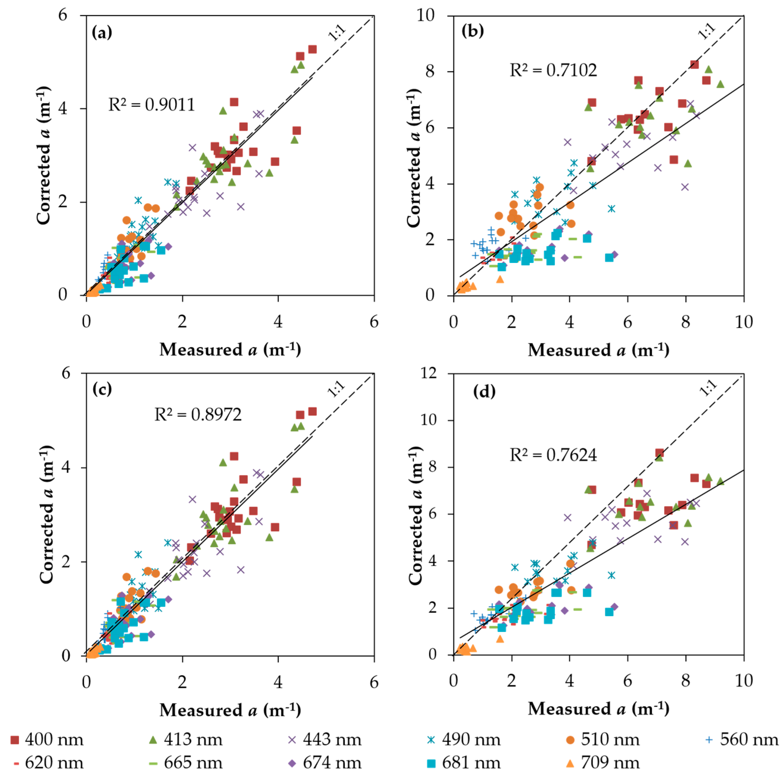
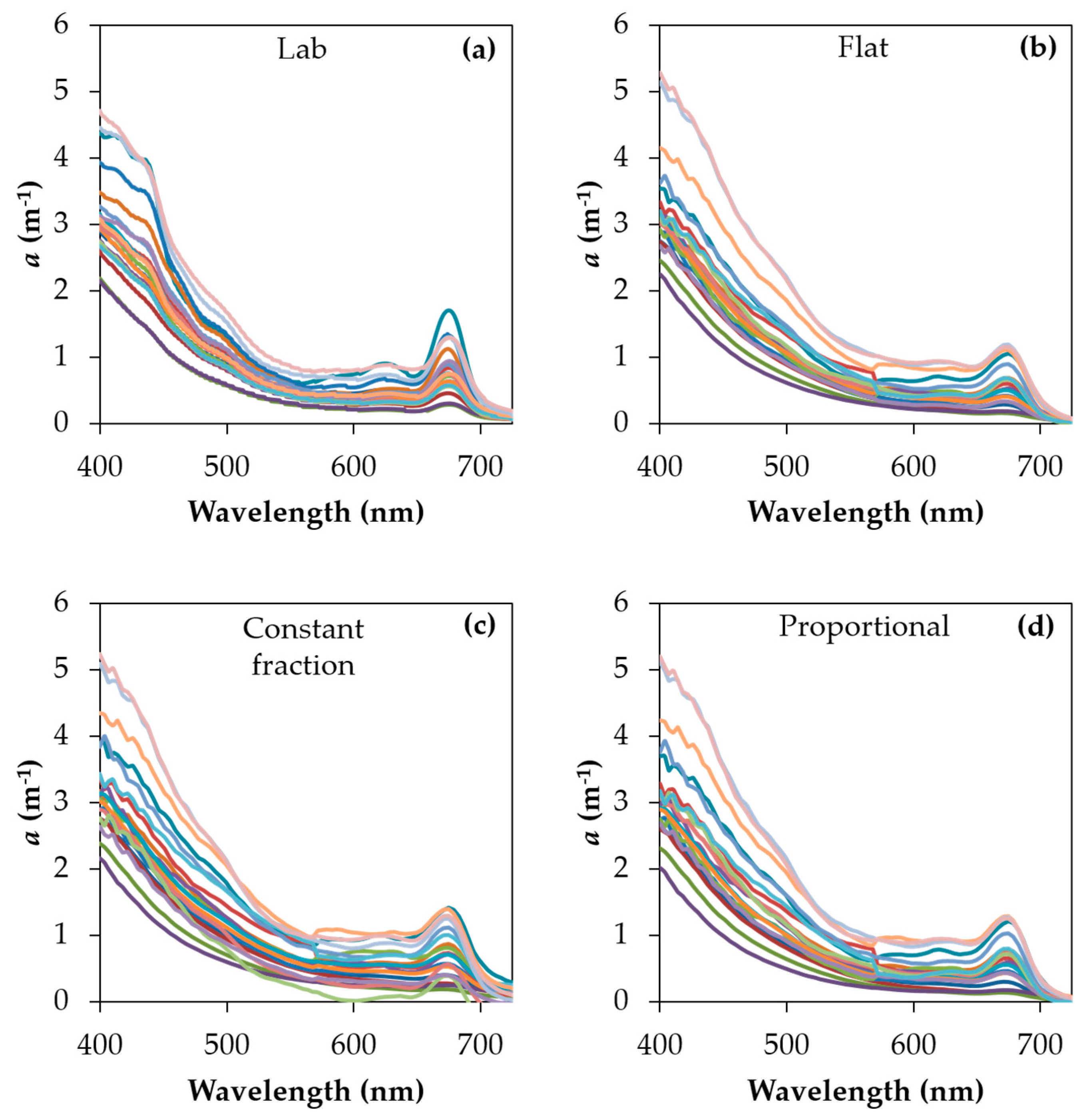
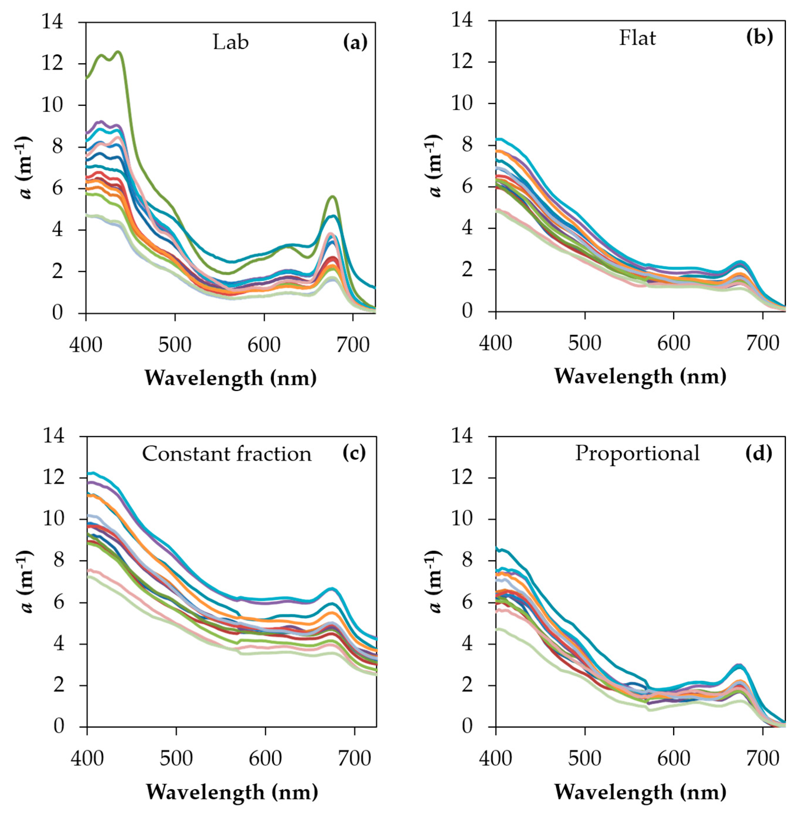
3.1. Scattering Error Correction

Table 1 shows the descriptive statistics of the optical water quality parameters collected in the May and October field campaigns. Overall, the dataset collected in October presented the highest values for chla and TSM concentrations. The BB reservoir showed a high trophic status in both periods, with an average chla content of 120.4 mg m−3 in May and 428.7 120.4 mg m−3 in October. On the other hand, TSM ranged from 3.6 g m−3 to 16.3 g m−3 in May, and from 10.8 g m−3 to 44 g m−3 in October. Such values directly influenced SDD measurements (average of 5.2 NTU for the first fieldwork and 0.6 for the second). It can be seen that the inorganic fraction (ISM) is much lower than the organic (OSM) at both dates.
Figure 2 shows the a(λ) curves that were estimated in the laboratory (Figure 2a) and collected by an ac-s meter and corrected using the flat (Figure 2b), constant fraction (Figure 2c), and proportional (Figure 2d) methods for the May dataset. Analyzing the a(λ) spectra, some spectral differences were identified between the May dataset and the a(λ) that was measured in the laboratory and corrected. It is worth noting that more discrete absorption features of phytoplankton pigments were found at 412 nm and 443 nm, exhibiting two peaks in the a(λ) spectra that was measured in the laboratory. In addition, the phycocyanin absorption feature at 620 nm was well defined in Figure 2a, while it was less obvious in the ac-s data. These differences may be caused by: (a) using different spectrophotometers; (b) collection at different depth; and (c) revolving water.
Regarding the variability of absorption measurements, samples 19 and 20 (see Figure 1 for location) exhibited the highest a(λ) spectra, both determined in the laboratory and collected in situ. Both samples were acquired in the Tietê River before its confluence with the Piracicaba River. Consistently, these points presented the highest chla concentrations in May (279.9 mg m−3 and 231.8 mg m−3 for 19 and 20, respectively). On the other hand, the lowest a(λ) spectrum determined in the laboratory (sample 4) also matched with the lowest ac-s spectrum and the second lowest chla content (26.2 mg m−3) observed in May. These results indicate that a(λ) variations are directly associated with phytoplankton biomass change.
In relation to scattering correction methods, negative values of a(λ) were derived using the constant fraction technique for sample 15 from 691 nm. It is clear that the constant factor of 0.18 was very high for this sample; however, no particular characteristics were observed in relation to chla and TSM content. Other methods also derived negative values, but just after λ0 (740 nm).
Figure 3 shows the a(λ) spectra determined in the laboratory (Figure 3a) and collected by ac-s and corrected using the flat (Figure 3b), constant fraction (Figure 3c), and proportional (Figure 3d) methods for the dataset acquired in October 2014. In this field campaign, two samples (3 and 14) showed a(λ) values that were much higher than the others, in the blue and red spectral regions, and were both associated with phytoplankton pigment absorption. As expected, these two samples presented the highest chla concentration (>700 mg m−3). On the other hand, the ac-s data did not show the same behavior as those estimated in the laboratory. Overall, the laboratory data magnitude was lower than the data that was measured using an ac-s sensor for the October dataset, probably due to: (1) a difference in collection depth; and (2) a deficiency of the correction method Analyzing the curves, the flat and proportional methods showed the best performance, lowering the magnitude of the spectra to a remarkable degree, while the constant fraction method yielded overestimations.
Table 2 shows the evaluation of the results produced by three scattering error corrections. The results exhibited a high variability in relation to the most suitable technique for each sample, especially for the May dataset. Nevertheless, overall, the flat method exhibited the best performance, with an average NRMSE of 7.95% and an average MAPE of 29.26% in May. On the other hand, in October, the proportional was the most suitable for most of the samples, with an average NRMSE of 11.20% and an average MAPE of 31.03%. NRMSE and MAPE values until approximately 30% were considered acceptable. Proportional techniques showed the best fit in terms of spectral shape, with a similarity of 0.098 rad for the May dataset, and 0.127 rad for the October dataset. Despite that, applying a paired t-student test, both the flat and proportional methods produced statistically similar results.

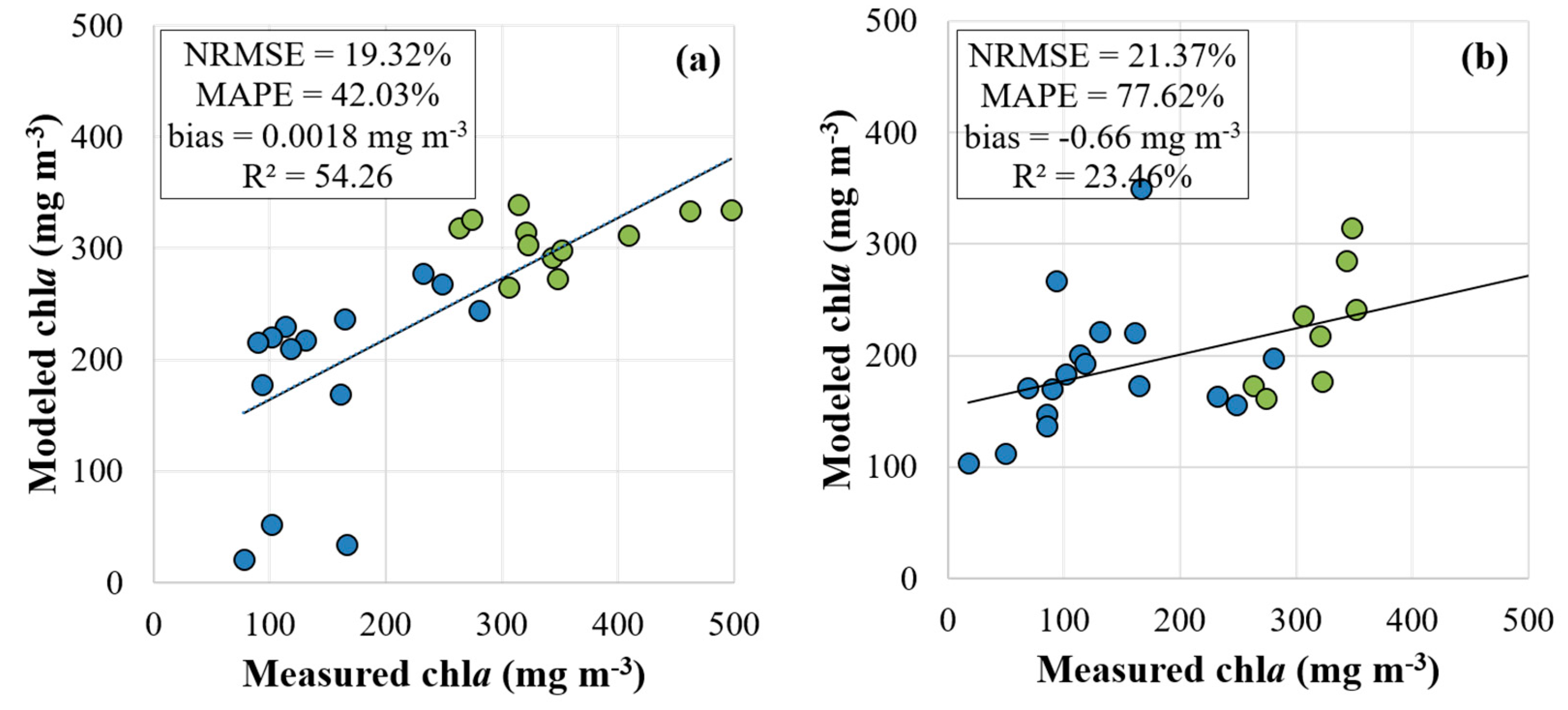
3.2. Implication in Modeling Chla Content

Due to the better performance in correcting scattering error, the a(λ) values that were derived from the flat and proportional methods were tested in estimating chla concentration. The algorithms were fitted simultaneously to both the May and October datasets. Some maximum and minimum values were pointed as outliers during the statistical analysis, taking into account a prediction interval of 95%. Regarding maximum values, it is likely that they are associated with the pigment packaging, as reported by Alcântara et al. [11]. This effect causes a(λ) spectrum flattening when there is an elevated phytoplankton biomass [14]. The blue and red regions are the main intervals affected [14], which can impair the performance of bio-optical models, since phytoplankton pigment and a(λ) do not increase proportionally.
Linear and polynomial adjustments were very similar for both algorithms; therefore, only the results produced by linear fit are given. Figure 4 shows the algorithms fitted to a(λ) that were corrected by the flat and proportional methods. Overall, both fits exhibit low errors, but the flat correction produced the best performance for chla estimation (NRMSE of 19.32% and MAPE of 42.03% for the flat data, and NRMSE of 21.37% and MAPE of 77.62% for the proportional data). Even though the bias is very close to zero for both corrected data, both a higher chla overestimation for the May dataset (lower chla content) and a higher underestimation in the October dataset (higher chla content) were noted.

4. Discussion

The results showed that the scattering error correction methods worked better when applied to the May dataset, i.e., for lower chla concentrations. This difference is clearer when analyzing the performance of constant fraction, which exhibited the worst results for both datasets. We obtained an average NRMSE of 9.25%, in May, which can be regarded as good result; on the other hand, the average NRMSE of 87.21% in October is unsatisfactory. A w of 0.18 produced accurate closure for May, while a higher w should have been adopted for October. Higher OSC concentrations not only increased the a(λ) measured by an ac-s meter, they also increased the b(λ) values inside the reflective tube. Consequently, the weights proposed for clear waters underestimate the true b(λ) fraction, and different weights are therefore needed to cover the high seasonal variability of the IOPs that are shown in Figure 2 and Figure 3. Carvalho et al. [25] tested different weights for turbid inland waters (Amazon River), establishing weights as high as 0.33.
On average, the flat technique produced good performance for the BB reservoir; however, we noted that it did not exhibit the best performance for all of the samples. The variation was higher in May, when the errors were lower. Although a(λ) and b(λ) were lower for the May dataset, the bio-optical variability was higher, as shown in Table 1. On the other hand, very high a(λ) and b(λ) values affected the performance of the methods, making it necessary to adopt higher weights (constant fraction) or shift the λ0 (flat and proportional). So, although the literature recommends avoiding wavelengths close to 745 nm as λ0, the use of 740 nm gave satisfactory results for the BB reservoir.
Pegau and Zaneveld [42] and Sullivan et al. [43] demonstrated the effects of temperature effects over aw(λ) and pointed to the wavelength at 745 nm as that most affected by temperature. In other words, aw(λ) increases with temperature, which can be confused with the a(λ) of other OSCs [42]. In clear water, 745 nm has a high influence over a(λ) due to its low magnitude. Nevertheless, in eutrophic inland waters, the temperature effect is reduced because of high a(λ) values. Also, using 715 nm as λ0 is not suitable for productive and turbid waters due to the high contribution of OSC absorption at that wavelength.
Statistically, the flat and proportional methods presented equal performance for the BB reservoir. However, a(λ) corrected by the flat model is more appropriate in estimating chla content. The best performance of the flat method in retrieving chla concentration must be associated with the proportion among the spectral absorption features, which are kept for this method. Corrected a(λ) can be used to design and access quasi-analytical [53] and semi-analytical algorithms [54], as well as applications in empirical models.
Figure 5 shows plots between measured and corrected a(λ) for the flat and proportional methods. A comparison was carried out for the first eleven bands of OLCI Sentinel-3 sensor (wavelengths centered at 400 nm, 412.5 nm, 442.5 nm, 490 nm, 510 nm, 560 nm, 620 nm, 665 nm, 673.75 nm, 681 nm, and 708.75 nm) [55]. These bands were selected because they are positioned at wavelengths that are associated with the absorption and scattering features of OSCs, which are widely used in remote sensing of the water color. Comparing scatterplots produced for the two methods, it is clear that the best performance is for May, which corroborates with the results shown in Table 2. The October dataset gives a higher dispersion of the samples, especially at shorter wavelengths (412.5 nm and 442.5 nm). Furthermore, the overestimation was also higher at shorter wavelengths.

5. Conclusions

Results showed that the flat and proportional methods gave the best performance in correcting the scattering in the reflective tube absorption meter of the ac-s meter in a highly productive reservoir. The first method showed better performance for lower a(λ) values (May dataset), while the second was better with the higher a(λ) values (October). On the other hand, according to results obtained with a SAM, the proportional method kept the spectral shape better. Although both flat and proportional methods have produced statistically similar results, the a(λ) values that were corrected by the first method yielded better chla estimations for both periods. In turn, the constant fraction technique produced an average NRMSE <10% for May, but considerably overestimated the October figures due to high IOP values. High bio-optical variability affects the selection of the best weight, since a unique value is not suitable for a large a(λ) range. In turn, constant fraction can be a practical technique for homogenous waters.
A strong relationship between bio-optical variability and the most suitable scattering correction method was also noticed. The May dataset exhibited the highest bio-optical variability, affecting the selection of the best method. However, every technique tested gave a better performance in May, when OSC concentrations and IOP values were lower. So, although the constant fraction predicted negative a(λ) values for one sample in May, in general, w = 0.018 was satisfactory for this dataset. Finally, although the proportional method exhibited the best performance in correcting a(λ) for the October dataset, chla estimating models worked better when a(λ) was corrected by the flat method. The t-student test showed that the flat and proportional methods exhibited statistically equal performances. Therefore, the application of flat method is therefore recommended for phytoplankton-dominated waters with a large chla range. For future works, an automatic selection of correction method could be developed for productive inland water based on the spectral characteristics of a(λ) values measured by an ac-s meter.

Author Contributions

Fernanda Watanabe, Thanan Rodrigues, Nariane Bernardo and Luiz Henrique Rotta carried out field surveys and did laboratorial analysis. Enner Alcântara and Nilton Imai managed the projects that funded the dataset acquisition and processing, as well as, supervising the first author respectively in Postdoc and Doctoral studies. Alisson do Carmo and Milton Shimabukuro developed the software architecture for ac-s data processing. Fernanda Watanabe conducted the experiments and wrote the paper; Enner Alcântara, Nariane Bernardo e Thanan Rodrigues corrected the manuscript.

Acknowledgments

The authors would like to thank the São Paulo Research Foundation (FAPESP Process Nos. 2012/19821-1, 2013/09045-7, 2015/21586-9 and 2015/18525-8), the National Council for Scientific and Technological Development (CNPq Process No. 472131/2012-5, 400881/2013-6 and 482605/2013-8). The authors also thank Edivaldo D. Velini and the staff of FCA/UNESP for allowing the use of their laboratory facilities. They also thank members of the SERTIE group (http://sertie.fct.unesp.br) from FCT/UNESP for all support in the field survey and laboratory.

Conflicts of Interest

The authors declare no conflicts of interest.

References

  1. Mobley, C.D. Light and Water: Radiative Transfer in Natural Waters; Academic Press: San Diego, CA, USA, 1994. [Google Scholar]
  2. Smith, R.C.; Baker, K.S. The bio-optical state of ocean waters and remote sensing. Limnol. Oceanogr. 1978, 23, 247–259. [Google Scholar] [CrossRef]
  3. Stramski, D.A.; Bricaud, A.; Morel, A. Modeling the inherent optical properties of the ocean based on the detailed composition of the planktonic community. Appl. Opt. 2001, 40, 2929–2945. [Google Scholar] [CrossRef] [PubMed]
  4. Babin, M.D.; Stramski, G.M.; Ferrari, G.M.; Claustre, H.; Bricaud, A.; Obolensky, G.; Hoepffner, N. Variations in the light absorption coefficients of phytoplankton, nonalgal particles, and dissolved organic matter in coastal waters around Europe. J. Geophys. Res. 2003, 108, 3211. [Google Scholar] [CrossRef]
  5. Bricaud, A.H.; Claustre, H.; Ras, J.; Oubelkheir, K. Natural variability of phytoplankton absorption in oceanic waters: Influence of the size structure of algal populations. J. Geophys. Res. 2004, 109, C11011. [Google Scholar] [CrossRef]
  6. Loos, E.A.; Costa, M. Inherent optical properties and optical mass classification of the waters of the Strait of Georgia, British Columbia, Canada. Prog. Oceanogr. 2010, 87, 144–156. [Google Scholar] [CrossRef]
  7. Campbell, G.; Phinn, S.R.; Daniel, P. The specific inherent optical properties of three sub-tropical and tropical water reservoirs in Queensland, Australia. Hydrobiologia 2011, 658, 233–252. [Google Scholar] [CrossRef]
  8. Wu, G.; Cui, L.; Duan, H.; Fei, T.; Liu, Y. Absorption and backscattering coefficients and their relations to water constituents of Poyang lake, China. Appl. Opt. 2011, 50, 6358–6368. [Google Scholar] [CrossRef] [PubMed]
  9. Ferreira, A.; Garcia, C.A.E.; Dogliotti, A.I.; Garcia, V.M.T. Bio-optical characteristics of the Patagonia Shelf break waters: Implications for ocean color algorithms. Remote Sens. Environ. 2013, 136, 416–432. [Google Scholar] [CrossRef]
  10. Riddick, C.A.L.; Hunter, P.D.; Tyler, A.N.; Martinez-Vicente, V.; Horváth, H.; Kovács, A.W.; Vörös, L.; Preston, T.; Présing, M. Spatial variability of absorption coefficients over a biogeochemical gradient in a large and optically complex shallow lake. J. Geophys. Res. Ocean. 2015, 120, 7040–7066. [Google Scholar] [CrossRef] [Green Version]
  11. Alcântara, E.; Watanabe, F.; Rodrigues, T.; Bernardo, N.; Rotta, L.; Carmo, A.; Curtarelli, M.; Imai, N. Field measurements of the backscattering coefficients in a cascading reservoir system: First results from Nova Avanhandava and Barra Bonita reservoirs (São Paulo, Brazil). Remote Sens. Lett. 2016, 7, 417–426. [Google Scholar] [CrossRef]
  12. Roesler, C.S.; Perry, M.J.; Carder, K.L. Modeling in situ phytoplankton absorption from total absorption spectra in productive inland marine waters. Limnol. Oceanogr. 1989, 34, 1510–1523. [Google Scholar] [CrossRef]
  13. Babin, M.; Therriault, J.C.; Legendre, L.; Condal, A. Variations in the specific absorption coefficient for natural phytoplankton assemblages: Impact on estimates of primary production. Limnol. Oceanogr. 1993, 38, 154–177. [Google Scholar] [CrossRef]
  14. Bricaud, A.; Babin, M.; Morel, A.; Claustre, H. Variability in the chlorophyll-specific absorption coefficients of natural phytoplankton: Analysis and parameterization. J. Geophys. Res. 1995, 100, 13321–13332. [Google Scholar] [CrossRef]
  15. Garcia, C.A.E.; Garcia, V.M.T.; Dogliotti, A.I.; Ferreira, A.; Romero, S.I.; Mannino, A.; Souza, M.S.; Matta, M.M. Environmental conditions and bio-optical signature of a cocolithophorid bloom in the Patagonian shelf. J. Geophys. Res. 2011, 116, C03025. [Google Scholar] [CrossRef]
  16. Lee, Z.P.; Carder, K.L.; Mobley, C.D.; Steward, R.G.; Patch, J.S. Hyperspectral remote sensing for shallow waters. I. A semianalytical model. Appl. Opt. 1998, 37, 6329–6338. [Google Scholar] [CrossRef] [PubMed]
  17. Gordon, H.R.; Brown, O.; Evans, R.H.; Brown, J.W.; Smith, R.C.; Baker, K.S.; Clark, D.K. A semianalytical radiance model of ocean color. J. Geophys. Res. 1988, 93, 10909–10924. [Google Scholar] [CrossRef]
  18. Canizzaro, J.P.; Carder, K.L. Estimating chlorophyll a concentration from remote-sensing reflectance in optically shallow waters. Remote Sens. Environ. 2006, 101, 13–24. [Google Scholar] [CrossRef]
  19. Tzortziou, M.; Subramaniam, A.; Herman, J.R.; Gallegos, C.L.; Neale, P.J.; Harding, L.W., Jr. Remote sensing reflectance and inherent optical properties in the mid Chesapeake bay. Estuar. Coast. Shelf 2007, 72, 16–32. [Google Scholar] [CrossRef]
  20. Carder, K.L.; Chen, F.R.; Lee, Z.P.; Hawes, S.K. Semianalytical Moderate-Resolution Imaging Spectrometer algorithm for chlorophyll a and absorption with bio-optical domains based on nitrate-depletion temperatures. J. Geophys. Res. 1999, 104, 5403–5421. [Google Scholar] [CrossRef]
  21. Brando, V.E.; Dekker, A.G. Satellite hyperspectral remote sensing for estimating estuarine and coastal water quality. IEEE Trans. Geosc. Remote Sens. 2003, 41, 1378–1387. [Google Scholar] [CrossRef]
  22. Gitelson, A.A.; Dall’Olmo, G.; Moses, W.; Rundquist, D.C.; Barrow, T.; Fisher, T.R.; Gurlin, D.; Holz, J. A simple semi-analytical model for remote estimation of chlorophyll-a in turbid waters: Validation. Remote Sens. Environ. 2008, 112, 3582–3593. [Google Scholar] [CrossRef]
  23. Mobley, C.D.; Sundman, L.K. Hydrolight 5.2, Ecolight 5.2: User’s Guide; Sequoia Scientific: Bellevue, WA, USA, 2013. [Google Scholar]
  24. Martinez-Vicente, V.; Land, P.E.; Tilstone, G.H.; Widdicombe, C.; Fishwich, J.R. Particulate scattering and backscattering related to water constituents and seasonal changes in the Western English channel. J. Plankton Res. 2010, 32, 603–619. [Google Scholar] [CrossRef]
  25. Carvalho, L.A.S.; Barbosa, C.C.F.; Novo, E.M.L.M.; Rudorff, C.M. Implications of scatter corrections for absorption measurements on optical closure of Amazon floodplain lakes using spectral absorption and attenuation meter (ac-s—WETLabs). Remote Sens. Environ. 2015, 157, 123–137. [Google Scholar] [CrossRef]
  26. Hout, Y.; Morel, A.; Twardowski, M.S.; Stramski, D.; Reynolds, A. Particle optical backscattering along a chlorophyll gradient in the upper layer of the eastern South Pacific ocean. Biogeosciences 2008, 5, 495–507. [Google Scholar] [CrossRef]
  27. Antoine, A.; Siegel, A.; Kostadinov, T.; Maritorena, S.; Nelson, N.B.; Gentili, B.; Vellucci, V.; Guilocheau, N. Variability optical particle backscattering in contrasting bio-optical oceanic regimes. Limnol. Oceanogr. 2011, 56, 955–973. [Google Scholar] [CrossRef]
  28. Zaneveld, J.R.; Kitchen, J.C.; Moore, C. The scattering error correction of reflecting-tube absorption meters. Proc. SPIE 1994, 2258, 44–55. [Google Scholar] [CrossRef]
  29. Kirk, J.T.O. Monte Carlo modeling of the performance of a reflective tube absorption meter. Appl. Opt. 1992, 31, 6463–6469. [Google Scholar] [CrossRef] [PubMed]
  30. Mckee, D.; Piskozub, J.; Brown, I. Scattering error corrections for in situ absorption and attenuation measurements. Opt. Express 2008, 16, 19480–19492. [Google Scholar] [CrossRef] [PubMed]
  31. Stockley, N.D.; Röttgers, R.; Mckee, D.; Fefering, I.; Sullivan, J.M.; Twardowski, M.S. Assessing uncertainties in scattering correction algorithms for reflective tube absorption measurements made with a WET Labs ac-9. Opt. Express 2017, 25, A1139. [Google Scholar] [CrossRef] [PubMed]
  32. Leymarie, E.; Doxaran, D.; Babin, M. Uncertainties associated to measurements of inherent optical properties in nature waters. Appl. Opt. 2010, 49, 5415–5436. [Google Scholar] [CrossRef] [PubMed]
  33. Röttgers, R.; Mckee, D.; Woźniak, B. Evaluation of scatter corrections for ac-9 absorption measurements in coastal waters. Methods Oceanogr. 2013, 7, 21–39. [Google Scholar] [CrossRef]
  34. Roesler, C.S. Theoretical and experimental approaches to improve the accuracy of particulate absorption coefficients derived from the quantitative filter technique. Limnol. Oceanogr. 1998, 43, 1649–1660. [Google Scholar] [CrossRef]
  35. Abe, D.S.; Matsumura-Tundisi, T.; Rocha, O.; Tundisi, G. Denitrification and bacterial community structure in the cascade of six reservoirs on a tropical river in Brazil. Hydrobiologia 2003, 504, 67–76. [Google Scholar] [CrossRef]
  36. Matsumura-Tundisi, T.; Tundisi, J.G. Plankton richness in a eutrophic reservoir (Barra Bonita reservoir, SP, Brazil). Hydrobiologia 2005, 542, 367–378. [Google Scholar] [CrossRef]
  37. Calijuri, M.C.; dos Santos, A.C.A. Short-term changes in the Barra Bonita reservoir (São Paulo, Brazil) emphasis on the phytoplankton communities. Hydrobiologia 1996, 330, 163–175. [Google Scholar] [CrossRef]
  38. Watanabe, F.S.Y.; Alcântara, E.H.; Rodrigues, T.W.P.; Bernardo, N.M.R.; Rotta, L.H.S.; Imai, N.N. Phytoplankton community dynamic detection from the chlorophyll-specific absorption coefficient in productive inland waters. Acta Limnol. Bras. 2017, 29, e13. [Google Scholar] [CrossRef]
  39. Dellamano-Oliveira, M.J.; Vieira, A.A.H.; Rocha, O.; Colombo, V.; Sant’Anna, C.L. Phytoplankton taxonomic composition and temporal changes in a tropical reservoir. Fundam. Appl. Limnol. 2008, 17, 27–38. [Google Scholar] [CrossRef]
  40. Tundisi, J.G.; Matsumura-Tundisi, T.; Pereira, K.C.; Luzia, A.P.; Passerini, M.D.; Chiba, W.A.C.; Morais, M.A.; Sebastian, N.Y. Cold fronts and reservoir limnology: An intergrated approach towards the ecological dynamics of freshwater ecosystems. Braz. J. Biol. 2010, 70, 815–824. [Google Scholar] [CrossRef] [PubMed]
  41. Barbosa, F.A.R.; Padisák, J.; Espíndola, E.L.; Borics, G.; Rocha, O. The cascading reservoirs continuum concept (CRCC) and its application to the rover Tietê-basin, São Paulo State, Brazil. In Theoretical Reservoir Ecology and Its Application; Tundisi, J.G., Straškraba, M., Eds.; International Institute of Ecology: São Carlos, Brazil, 1999; pp. 425–437. [Google Scholar]
  42. Pegau, W.S.; Zaneveld, R.V. Temperature-dependent absorption of water in the red and near-infrared portions of the spectrum. Limnol. Oceanogr. 1993, 38, 188–192. [Google Scholar] [CrossRef]
  43. Sullivan, J.M.; Twardowski, M.S.; Zaneveld, R.V.; Moore, C.M.; Bernard, A.H.; Donaghay, P.L.; Rhoades, B. Hyperspectral temperature and salt dependencies of absorption by water and heavy water in the 400–750 nm spectral range. Appl. Opt. 2006, 45, 5294–5309. [Google Scholar] [CrossRef] [PubMed]
  44. Imai, N.N.; Shimabukuro, M.H.; Carmo, A.F.C.; Alcântara, E.H.; Rodrigues, T.; Watanabe, F. Bio-optical data integration based on a 4 D database system approach. Int. Arch. Photogramm. Remote Sens. Spat. Inf. Sci. 2015, XL-7/W3, 635–641. [Google Scholar] [CrossRef]
  45. Tassan, S.; Ferrari, G.M. An alternative approach to absorption measurements of aquatic particles retained on filters. Limnol. Oceanogr. 1995, 40, 1358–1368. [Google Scholar] [CrossRef]
  46. Tassan, S.; Ferrari, G.M. Measurements of light absorption by aquatic particles retained on filters: Determination of the optical path length amplification by the ‘transmittance-reflectance’ method. J. Plankton Res. 1998, 20, 1699–1709. [Google Scholar] [CrossRef]
  47. Tassan, S.; Ferrari, G.M. A sensitivity analysis of the ‘transmittance-reflectance’ method for measuring light absorption by aquatic particles. J. Plankton Res. 2002, 24, 757–774. [Google Scholar] [CrossRef]
  48. Cleveland, J.S.; Weidemann, A.D. Quantifying absorption by aquatic particles: A multiple scattering correction for glass-fiber filters. Limnol. Oceanogr. 1993, 38, 1321–1327. [Google Scholar] [CrossRef]
  49. Bricaud, A.; Morel, A.; Prieur, L. Absorption by dissolved organic matter of the sea (yellow substance) in the UV and visible domains. Limnol. Oceanogr. 1981, 26, 43–53. [Google Scholar] [CrossRef]
  50. Golterman, H.L.; Clymo, R.S.; Ohnstad, M.A.M. Methods for Physical and Chemical Analysis of Fresh Water; Blackwell Scientific Publications: Oxford, UK, 1978. [Google Scholar]
  51. American Public Health Association (APHA); American Water Works Association (AWWA); Water Environmental Federation (WEF). Standard Methods for the Examination of Water and Wastewater, 20th ed.; APHA; AWWA; WEF: Washington, DC, USA, 1998; pp. 2–54. [Google Scholar]
  52. Kruse, F.A.; Lefkoff, A.B.; Boardman, J.W.; Heidebrecht, K.B.; Shapiro, A.T.; Barloon, P.J.; Goetz, A.F.H. The spectral image processing system (SIPS)—interactive visualization and analysis of imaging spectrometer data. Remote Sens. Environ. 1993, 44, 145–163. [Google Scholar] [CrossRef]
  53. Lee, Z.P.; Carder, K.L. Absorption spectrum of phytoplankton pigments derived from hyperspectral remote-sensing reflectance. Remote Sens. Environ. 2004, 89, 361–368. [Google Scholar] [CrossRef]
  54. Watanabe, F.; Alcântara, A.; Imai, N.; Rodrigues, T.; Bernardo, N. Estimation of chlorophyll-a concentration from optimizing a semi-analytical algorithm in productive inland waters. Remote Sens. 2018, 10, 227. [Google Scholar] [CrossRef]
  55. Donlon, C.; Berruti, B.; Buongiorno, A.; Ferreira, M.H.; Féménias, P.; Frerick, J.; Goryl, P.; Klein, U.; Laur, H.; Mavrocordatos, C.; et al. The global monitoring for environment and security (GMES) Sentinel-3 mission. Remote Sens. Environ. 2012, 120, 37–57. [Google Scholar] [CrossRef]
Figure 1. The Barra Bonita (BB) hydroelectric reservoir lies on (a) a cascading reservoir system in the Tietê River, (b) in São Paulo State, Brazil. Sampling stations randomly distributed along the reservoir for (c) May and (d) October field campaigns.
Remotesensing 10 00740 g001
Figure 2. Measurements of a(λ) obtained by (a) laboratory spectrophotometry and acquired by an absorption and attenuation spectral (ac-s) meter and previously corrected using (b) flat, (c) constant fraction, and (d) proportional methods for the dataset collected in May 2014.
Remotesensing 10 00740 g002
Figure 3. Measurements of a(λ) obtained by (a) laboratory spectrophotometry and acquired by an ac-s meter and previously corrected using (b) the flat, (c) constant fraction, and (d) proportional methods for the dataset collected in October 2014.
Remotesensing 10 00740 g003
Figure 4. Chla retrieval algorithm fitted using a(λ) values that were derived from scattering correction methods: (a) flat and (b) proportional.
Remotesensing 10 00740 g004
Figure 5. Measurements of a(λ) obtained by spectrophotometry in the laboratory and acquired by an ac-s meter, and previously corrected using the flat method applied to the (a) May and (b) October datasets, and using the proportional method applied to the (c) May and (d) October datasets.
Remotesensing 10 00740 g005
Table 1. Descriptive statistics of water quality optical parameters: chla (mg m−3), TSM, inorganic suspended matter (ISM), and organic suspended matter (OSM) (g m−3), Secchi disk depth (SDD) (m) and turbidity (NTU) collected in May and October 2014. Statistics metrics used: minimum value (Min), maximum value (Max), mean, standard deviation (SD), and coefficient of variation (CV = (SD/mean) × 100) (%).
ParameterMinMaxMeanSDCV
Dataset collected on 5–9 May 2014, n = 20 samples
Chla17.7279.9120.470.358.4
TSM3.616.37.23.345.8
ISM0.24.41.10.978.8
OSM2.814.76.13.252.0
SDD0.82.31.50.426.7
Turbidity1.712.55.22.446.2
Dataset collected on 13–16 October 2014, n = 15 samples
Chla263.2797.8415.4159.238.3
TSM10.844.023.57.431.7
ISM0.63.82.51.040.9
OSM10.230.419.54.824.6
SDD0.370.780.560.1119.1
Turbidity15.133.219.85.226.3
Table 2. Assessment of the scattering error correction methods for the datasets collected in May and October 2014 using root mean square error (RMSE) (m−1), normalized root mean square error (NRMSE) (%), mean absolute percentage error (MAPE) (%), bias (m−1), and a Spectral Angle Mapper (SAM) (rad).
MethodRMSENRMSEMAPEbiasSAM
Correction for May 2014
Flat0.2577.9529.260.0480.103
Constant fraction0.2929.2549.201.1270.199
Proportional0.2638.2230.570.0530.098
Correction for October 2014
Flat0.96913.0334.89−0.1820.154
Constant fraction3.12448.14859.843.0460.348
Proportional0.83311.2031.03−0.1310.127

