Applying Independent Component Analysis on Sentinel-2 Imagery to Characterize Geomorphological Responses to an Extreme Flood Event near the Non-Vegetated Río Colorado Terminus, Salar de Uyuni, Bolivia


Abstract
1. Introduction
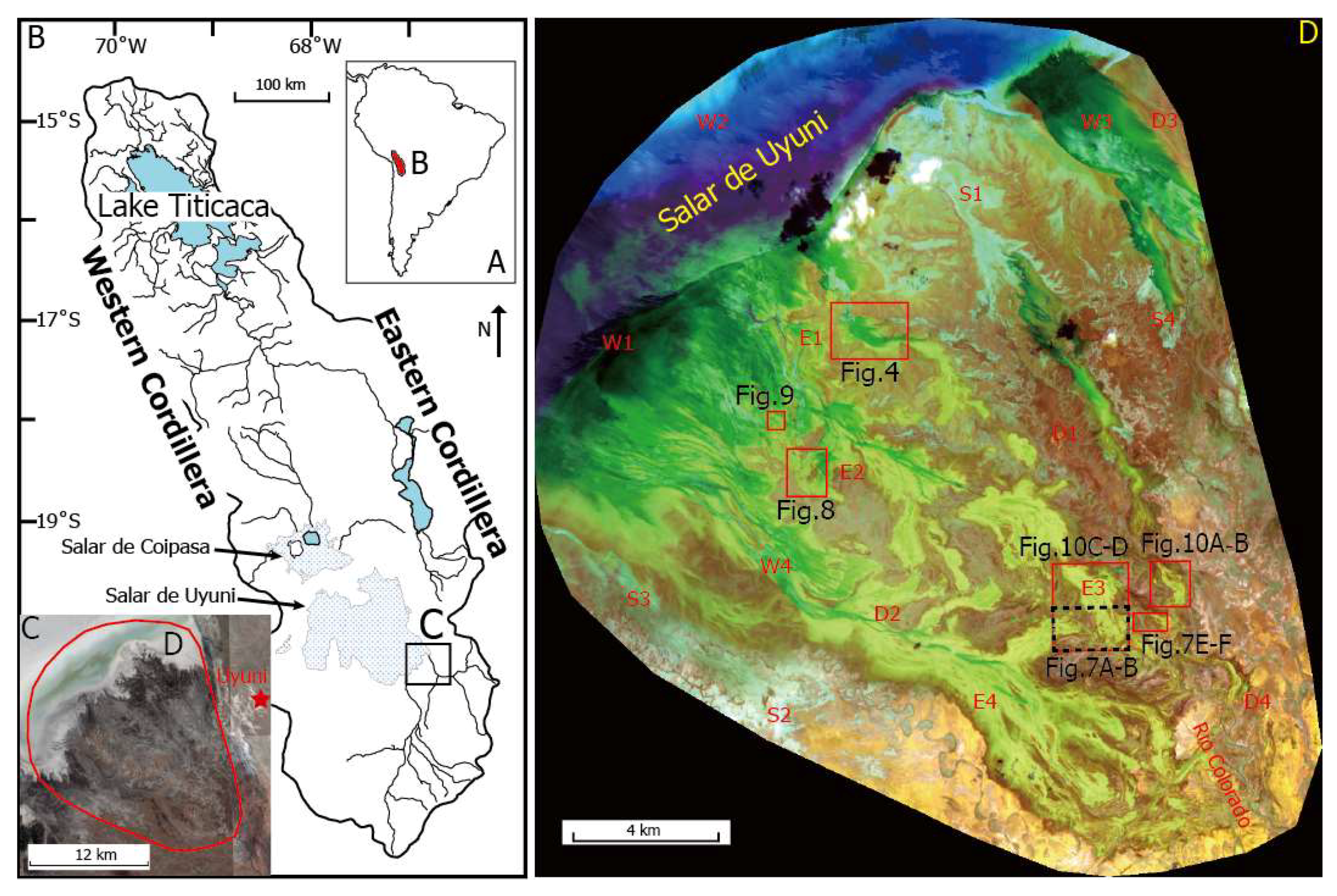
2. Study Area
3. Materials and Methods
3.1. Materials
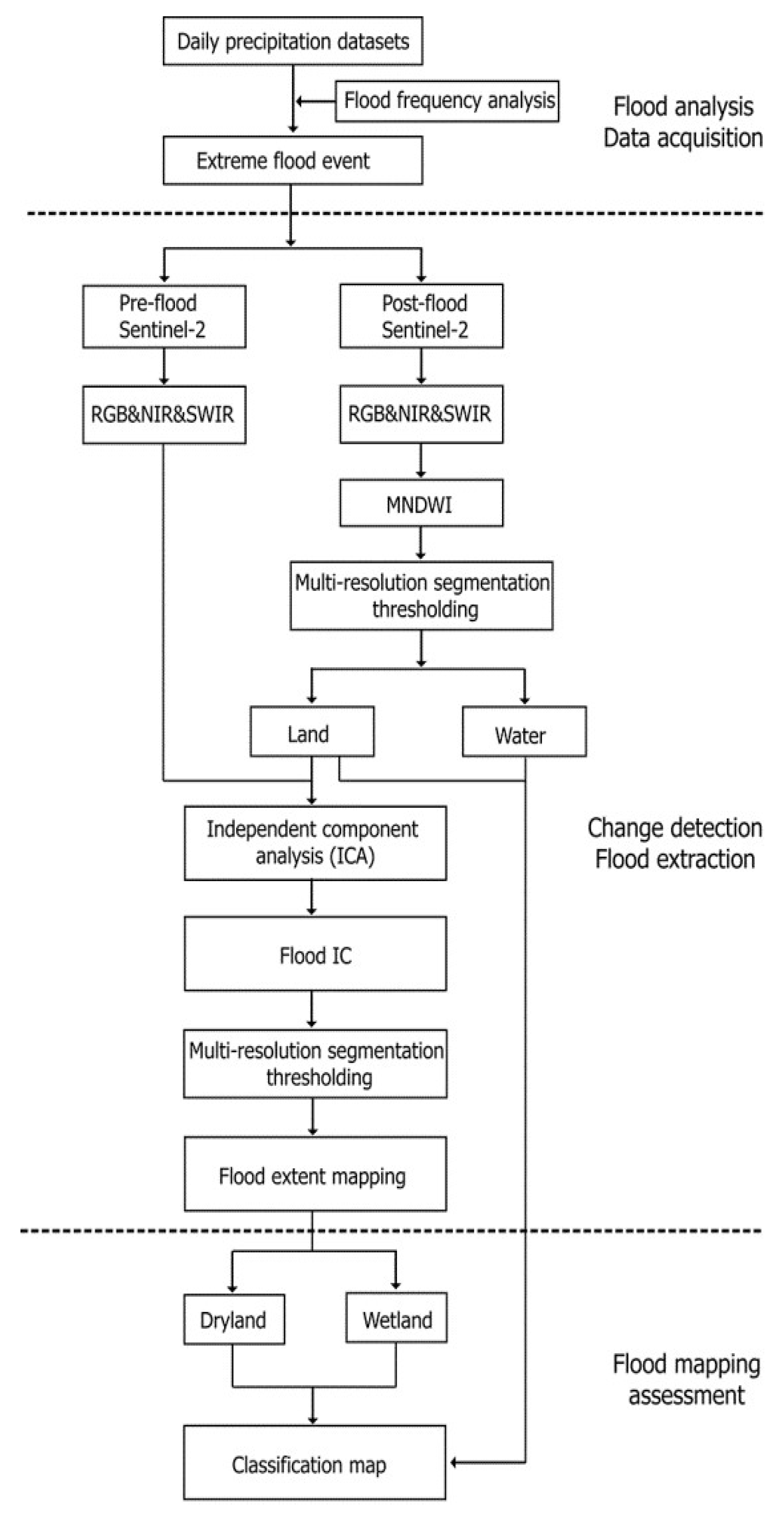
3.2. Methodology
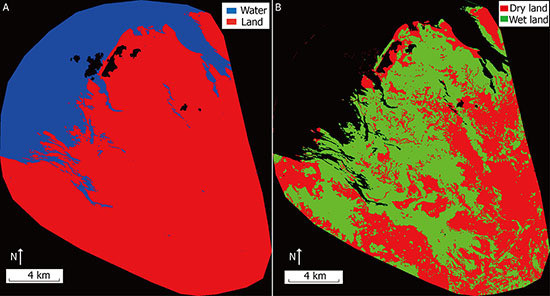
4. Results
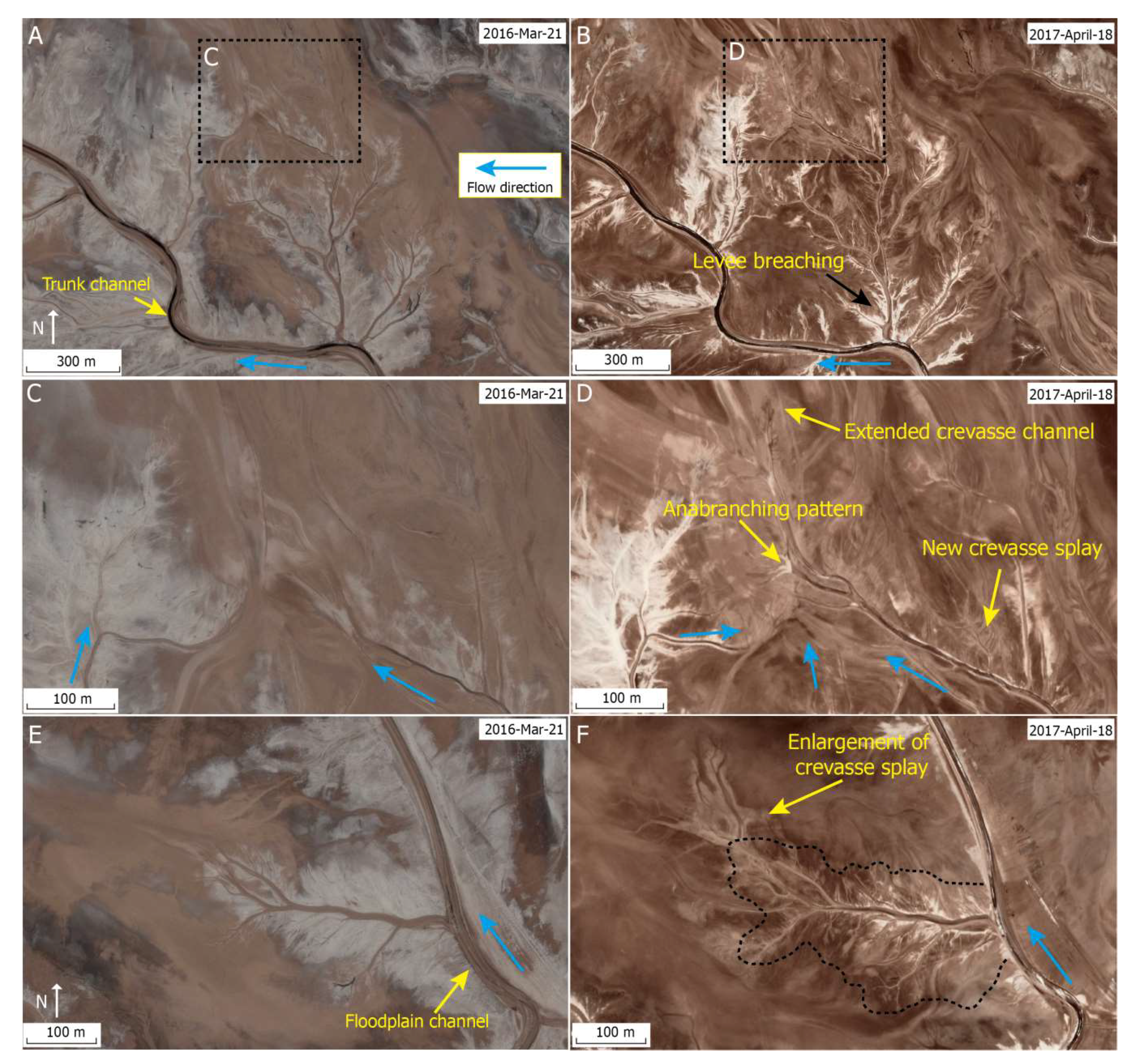
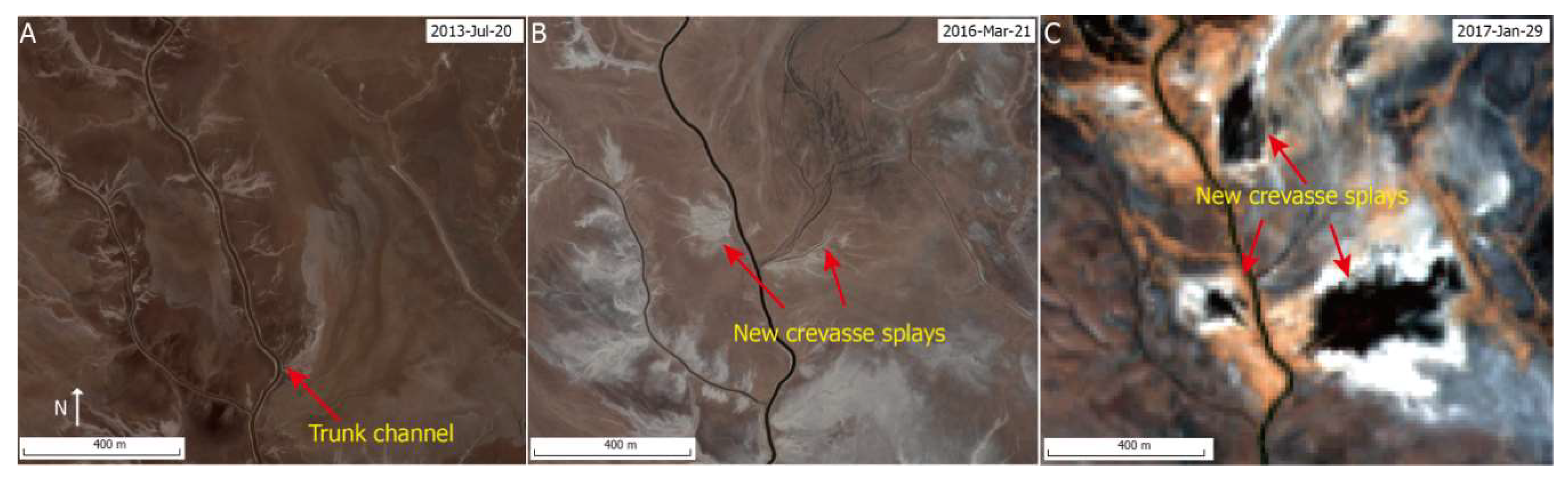
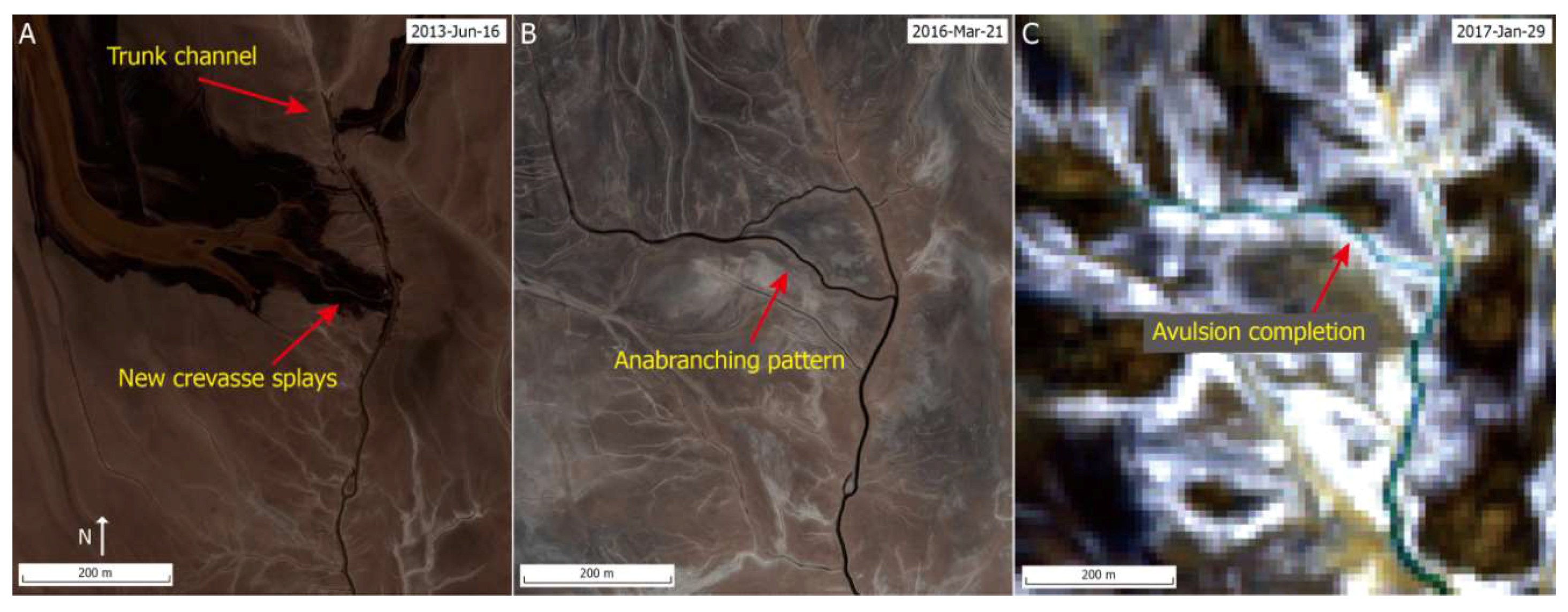
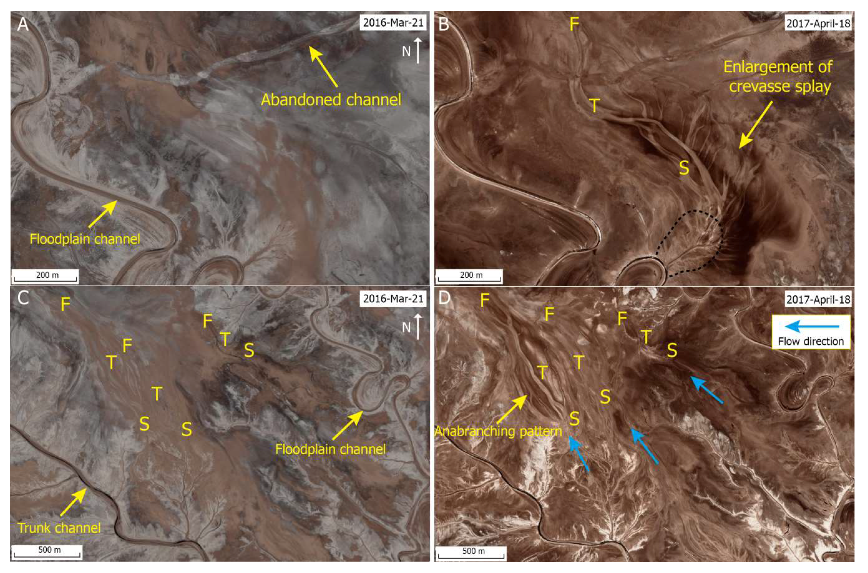
4.1. Visual Interpretation
4.2. Accuracy Assessment
4.3. Flood Extent, Flood Patterns, and Geomorphological Changes
5. Interpretation and Discussion
5.1. Strengths and Limitations
5.2. Morphodynamics Resulting from Extreme Flood Events in Terminal Dryland River Systems
6. Conclusions
Author Contributions
Funding
Acknowledgments
Conflicts of Interest
References
- Shaw, P.A.; Bryant, R.G. Playas, pans and salt lakes. In Arid Zone Geomorphology: Process, Form and Change in Drylands, 3rd ed.; Thomas, D.S.G., Ed.; John Wiley & Sons, Ltd.: Chichester, UK, 2011; pp. 373–401. [Google Scholar]
- Tooth, S.; Nanson, G.C. Distinctiveness and diversity of arid zone river systems. In Arid Zone Geomorphology: Process, Form and Change in Drylands, 3rd ed.; Thomas, D.S.G., Ed.; John Wiley & Sons, Ltd.: Chichester, UK, 2011; pp. 269–300. [Google Scholar]
- Reid, I.; Frostick, L.E. Channel Form, Flows and Sediments in Deserts. In Arid Zone Geomorphology: Process, Form and Change in Drylandss, 2nd ed.; Thomas, D.S.G., Ed.; Wiley: Chichester, UK, 1997; pp. 205–229. [Google Scholar]
- Lang, S.C.; Payenberg, T.H.D.; Reilly, M.R.W.; Hicks, T.; Benson, J.; Kassan, J. Modern Analogues for Dryland Sandy Fluvial-Lacustrine Deltas and Terminal Splay Reservoirs. APPEA J. 2004, 44, 329. [Google Scholar] [CrossRef]
- Fisher, J.A.; Krapf, C.B.E.; Lang, S.C.; Nichols, G.J.; Payenberg, T.H.D. Sedimentology and architecture of the Douglas Creek terminal splay, Lake Eyre, central Australia. Sedimentology 2008, 55, 1915–1930. [Google Scholar] [CrossRef]
- Bryant, R.G. Validated linear mixture modelling of landsat TM data for mapping evaporite minerals on a playa surface: Methods and applications. Int. J. Remote Sens. 1996, 17, 315–330. [Google Scholar] [CrossRef]
- Zartman, R.E.; Ramsey, R.H.; Evans, P.W.; Koenig, G.; Truby, C.; Kamara, L. Outerbasin, annulus and playa basin infiltration studies. Texas J. Agric. Nat. Resour. 1996, 9. [Google Scholar]
- Bartuszevige, A.M.; Pavlacky, D.C.; Burris, L.; Herbener, K. Inundation of playa wetlands in the western Great Plains relative to landcover context. Wetlands 2012, 32, 1103–1113. [Google Scholar] [CrossRef]
- Smith, L.M. Playas of the Great Plains; University of Texas Press: Austin, TX, USA, 2003. [Google Scholar]
- Sirisena, K.A.; Ramirez, S.; Steele, A.; Glamoclija, M. Microbial Diversity of Hypersaline Sediments from Lake Lucero Playa in White Sands National Monument, New Mexico, USA. Microb. Ecol. 2018, 1–15. [Google Scholar] [CrossRef] [PubMed]
- McKie, T. A Comparison of Modern Dryland Depositional Systems with the Rotliegend Group in the Netherlands. In The Permian Rotliegend of The Netherlands; SEPM Society for Sedimentary Geology: Darlington, UK, 2011; pp. 89–103. [Google Scholar]
- Van Toorenenburg, K.A.; Donselaar, M.E.; Noordijk, N.A.; Weltje, G.J. On the origin of crevasse-splay amalgamation in the Huesca fluvial fan (Ebro Basin, Spain): Implications for connectivity in low net-to-gross fluvial deposits. Sediment. Geol. 2016, 343, 156–164. [Google Scholar] [CrossRef]
- Pickup, G. The erosion cell—A geomorphic approach to landscape classification in range assessment. Rangel. J. 1985, 7, 114–121. [Google Scholar] [CrossRef]
- Pickup, G. Event frequency and landscape stability on the floodplain systems of arid Central Australia. Quat. Sci. Rev. 1991, 10, 463–473. [Google Scholar] [CrossRef]
- Wakelin-King, G.A.; Webb, J.A. Threshold-dominated fluvial styles in an arid-zone mud-aggregate river: The uplands of Fowlers Creek, Australia. Geomorphology 2007, 85, 114–127. [Google Scholar] [CrossRef]
- Tooth, S.; McCarthy, T.; Rodnight, H.; Keen-Zebert, A.; Rowberry, M.; Brandt, D. Late Holocene development of a major fluvial discontinuity in floodplain wetlands of the Blood River, eastern South Africa. Geomorphology 2014, 205, 128–141. [Google Scholar] [CrossRef]
- Woodward, J.C.; Tooth, S.; Brewer, P.A.; Macklin, M.G. The 4th International Palaeoflood Workshop and trends in palaeoflood science. Glob. Planet. Chang. 2010, 70, 1–4. [Google Scholar] [CrossRef]
- Bates, P.D.; Horritt, M.S.; Smith, C.N.; Mason, D. Integrating remote sensing observations of flood hydrology and hydraulic modelling. Hydrol. Process. 1997, 11, 1777–1795. [Google Scholar] [CrossRef]
- Houser, P.R.; Shuttleworth, W.J.; Famiglietti, J.S.; Goodrich, D.C. Integration of soil moisture remote sensing and hydrologic modelling using data assimilation. Water Resour. Manag. 1998, 34, 3405–3420. [Google Scholar] [CrossRef]
- Balenzano, A.; Satalino, G.; Belmonte, A.; D’Urso, G.; Capodici, F.; Iacobellis, V. On the Use of Multi-Temporal Series of COSMO-SkyMed Data for Landcover Classification and Surface Parameter Retrieval over Agricultural Sites. In Proceedings of the 2011 IEEE Geoscience and Remote Sensing Symposium (IGARSS2011), Vancouver, BC, Canada, 24–29 July 2011; pp. 142–145. [Google Scholar]
- Tarantino, E.; Novelli, A.; Laterza, M.; Gioia, A.; Politecnico, D.; Orabona, V. Testing high spatial resolution WorldView-2 Imagery for retrieving the Leaf Area Index. Proc. SPIE 2015, 9535, 1–8. [Google Scholar]
- Islam, A.S.; Bala, S.K.; Haque, M.A. Flood inundation map of Bangladesh using MODIS time-series images. J. Flood Risk Manag. 2010, 3, 210–222. [Google Scholar] [CrossRef]
- Huang, C.; Chen, Y.; Wu, J. Mapping spatio-temporal flood inundation dynamics at large river basin scale using time-series flow data and MODIS imagery. Int. J. Appl. Earth Obs. Geoinf. 2014, 26, 350–362. [Google Scholar] [CrossRef]
- Chignell, S.M.; Anderson, R.S.; Evangelista, P.H.; Laituri, M.J.; Merritt, D.M. Multi-temporal independent component analysis and Landsat 8 for delineating maximum extent of the 2013 Colorado front range flood. Remote Sens. 2015, 7, 9822–9843. [Google Scholar] [CrossRef]
- Hyvarinen, A. Fast and robust fixed-point algorithm for independent component analysis. IEEE Trans. Neural Netw. Learn. Syst. 1999, 10, 626–634. [Google Scholar] [CrossRef] [PubMed]
- Hyvärinen, A.; Oja, E. Independent Component Analysis: Algorithms and Applications. Neural Netw. 2000, 13, 411–430. [Google Scholar] [CrossRef]
- Drusch, M.; Del Bello, U.; Carlier, S.; Colin, O.; Fernandez, V.; Gascon, F.; Hoersch, B.; Isola, C.; Laberinti, P.; Martimort, P. Sentinel-2: ESA’s Optical High-Resolution Mission for GMES Operational Services. Remote Sens. Environ. 2012, 120, 25–36. [Google Scholar] [CrossRef]
- Yang, X.; Zhao, S.; Qin, X.; Zhao, N.; Liang, L. Mapping of urban surface water bodies from sentinel-2 MSI imagery at 10 m resolution via NDWI-based image sharpening. Remote Sens. 2017, 9, 596. [Google Scholar] [CrossRef]
- Yang, X.; Chen, L. Evaluation of automated urban surface water extraction from Sentinel-2A imagery using different water indices. J. Appl. Remote Sens. 2017, 11, 26016. [Google Scholar] [CrossRef]
- Marshall, L.G.; Swisher, C.C., III; Lavenu, A.; Hoffstetter, R.; Curtis, G.H. Geochronology of the mammal-bearing late Cenozoic on the northern Altiplano, Bolivia. J. S. Am. Earth Sci. 1992, 5, 1–19. [Google Scholar] [CrossRef]
- Horton, B.K.; Decelles, P.G. Modern and ancient fluvial megafans in the foreland basin system of the central Andes, southern Bolivia: Implications for drainage network evolution in fold-thrust belts. Basin Res. 2001, 13, 43–63. [Google Scholar] [CrossRef]
- Baucom, P.C.; Rigsby, C.A. Climate and lake-level history of the northern Altiplano, Bolivia, as recorded in Holocene sediments of the Rio Desaguadero. J. Sediment. Res. 1999, 69, 597–611. [Google Scholar] [CrossRef]
- Bills, B.G.; De Silva, S.L.; Currey, D.R.; Emenger, R.S.; Lillquist, K.D.; Donnellan, A.; Worden, B. Hydro-isostatic deflection and tectonic tilting in the central Andes: Initial results of a GPS survey of Lake Minchin shorelines. Geophys. Res. Lett. 2013, 21, 293–296. [Google Scholar] [CrossRef]
- Placzek, C.J.; Quade, J.; Patchett, P.J. A 130 ka reconstruction of rainfall on the Bolivian Altiplano. Earth Planet. Sci. Lett. 2013, 363, 97–108. [Google Scholar] [CrossRef]
- Argollo, J.; Mourguiart, P. Late Quaternary climate history of the Bolivian Altiplano. Quat. Int. 2000, 72, 37–51. [Google Scholar] [CrossRef]
- Grosjean, M. Paleohydrology of Laguna Lejia (north Chilean Altiplano) and climatic implications for Late Glacial times. Palaeogeogr. Palaeoclimatol. Palaeoecol. 1994, 109, 89–100. [Google Scholar] [CrossRef]
- Risacher, F.; Fritz, A.B.; Lerman, A. Origin of salts and brine evolution of Bolivian and Chilean salars. Aquat. Geochem. 2009, 15, 123–157. [Google Scholar] [CrossRef]
- Lenters, J.D.; Cook, K.H. Summertime Precipitation Variability over South America: Role of the Large-Scale Circulation. Mon. Weather Rev. 1999, 127, 409–431. [Google Scholar] [CrossRef]
- Li, J.; Donselaar, M.E.; Hosseini Aria, S.E.; Koenders, R.; Oyen, A.M. Landsat imagery-based visualization of the geomorphological development at the terminus of a dryland river system. Quat. Int. 2014, 352, 100–110. [Google Scholar] [CrossRef]
- Li, J.; Menenti, M.; Mousivand, A.; Luthi, S.M. Non-vegetated playa morphodynamics using multi-temporal landsat imagery in a semi-arid endorheic basin: Salar de Uyuni, Bolivia. Remote Sens. 2014, 6, 10131–10151. [Google Scholar] [CrossRef]
- Li, J.; Luthi, S.M.; Donselaar, M.E.; Weltje, G.J.; Prins, M.A.; Bloemsma, M.R. An ephemeral meandering river system: Sediment dispersal processes in the Río Colorado, Southern Altiplano Plateau, Bolivia. Z. Geomorphol. 2015, 59, 301–317. [Google Scholar] [CrossRef]
- Toming, K.; Kutser, T.; Laas, A.; Sepp, M.; Paavel, B.; Nõges, T. First experiences in mapping lakewater quality parameters with sentinel-2 MSI imagery. Remote Sens. 2016, 8, 640. [Google Scholar] [CrossRef]
- Escolà, A.; Badia, N.; Arnó, J.; Martínez-Casasnovas, J.A. Using Sentinel-2 images to implement Precision Agriculture techniques in large arable fields: First results of a case study. Adv. Anim. Biosci. 2017, 8, 377–382. [Google Scholar] [CrossRef]
- Louis, J.; Debaecker, V.; Pflug, B.; Mainkorn, M.; Bieniarz, J.; Muellerwilm, U.; Cadau, E.; Gascon, F. Sentinel-2 Sen2Cor: L2A Processor for Users. In Proceedings of the Living Planet Symposium, Prague, Czech Republic, 9–13 May 2016. [Google Scholar]
- Li, J.; Bristow, C.S. Crevasse splay morphodynamics in a dryland river terminus: Río Colorado in Salar de Uyuni Bolivia. Quat. Int. 2015, 377, 71–82. [Google Scholar] [CrossRef]
- Xu, H. Modification of normalised difference water index (NDWI) to enhance open water features in remotely sensed imagery. Int. J. Remote Sens. 2006, 27, 3025–3033. [Google Scholar] [CrossRef]
- Du, Y.; Zhang, Y.; Ling, F.; Wang, Q.; Li, W.; Li, X. Water bodies’ mapping from Sentinel-2 imagery with Modified Normalized Difference Water Index at 10-m spatial resolution produced by sharpening the swir band. Remote Sens. 2016, 8, 354. [Google Scholar] [CrossRef]
- Wang, J.Z.; Li, J.; Gray, R.M.; Wiederhold, G. Unsupervised multiresolution on segmentation for images with low depth of field. IEEE Trans. Pattern Anal. Mach. Intell. 2001, 23, 85–90. [Google Scholar] [CrossRef]
- Blaschke, T. Object based image analysis for remote sensing. ISPRS J. Photogramm. Remote Sens. 2010, 65, 2–16. [Google Scholar] [CrossRef]
- Belgiu, M.; Drǎguţ, L. Comparing supervised and unsupervised multiresolution segmentation approaches for extracting buildings from very high resolution imagery. ISPRS J. Photogramm. Remote Sens. 2014, 96, 67–75. [Google Scholar] [CrossRef] [PubMed]
- Zhong, J.; Wang, R. Multi-temporal remote sensing change detection based on independent component analysis. Int. J. Remote Sens. 2006, 27, 2055–2061. [Google Scholar] [CrossRef]
- Lobell, D.B.; Asner, G.P. Moisture effects on soil reflectance. Soil Sci. Soc. Am. J. 2002, 66, 722–727. [Google Scholar] [CrossRef]
- Kaplan, G.; Avdan, U. Object-based water body extraction model using Sentinel-2 satellite imagery. Eur. J. Remote Sens. 2017, 50. [Google Scholar] [CrossRef]
- Donselaar, M.E.; Gozalo, M.C.C.; Moyano, S. Avulsion processes at the terminus of low-gradient semi-arid fl uvial systems: Lessons from the Río Colorado, Altiplano endorheic basin, Bolivia. Sediment. Geol. 2013, 283, 1–14. [Google Scholar] [CrossRef]
- Bourke, M.C.; Pickup, G. Fluvial form variability in arid central Australia. In Varieties of Fluvial Form; Miller, A.J., Gupta, A., Eds.; John Wiley & Sons, Ltd.: Chichester, UK, 1999; pp. 249–271. [Google Scholar]
- Tooth, S. Splay Formation Along the Lower Reaches of Ephemeral Rivers on the Northern Plains of Arid Central Australia. J. Sediment. Res. 2005, 75, 636–649. [Google Scholar] [CrossRef]
- Li, J.; Tooth, S.; Yao, G. Channel-floodplain morphodynamics in low-gradient, non-vegetated reaches near a dryland river terminus: Salar de Uyuni, Bolivia. Earth Surf. Process. Landf. 2018. in review. [Google Scholar]


| Sentinel-2 Bands | Central Wavelength (µm) | Resolution (m) | Bandwidth (nm) |
|---|---|---|---|
| Band 1—Coastal aerosol | 0.443 | 60 | 20 |
| Band 2—Blue | 0.490 | 10 | 65 |
| Band 3—Green | 0.560 | 10 | 35 |
| Band 4—Red | 0.665 | 10 | 30 |
| Band 5—Vegetation Red Edge | 0.705 | 20 | 15 |
| Band 6—Vegetation Red Edge | 0.740 | 20 | 15 |
| Band 7—Vegetation Red Edge | 0.783 | 20 | 20 |
| Band 8—NIR | 0.842 | 10 | 115 |
| Band 8A—Narrow NIR | 0.865 | 20 | 20 |
| Band 9—Water vapour | 0.945 | 60 | 20 |
| Band 10—SWIR—Cirrus | 1.380 | 60 | 30 |
| Band 11—SWIR | 1.610 | 20 | 90 |
| Band 12—SWIR | 2.190 | 20 | 180 |
| Type | Catalog ID | Acq. Date | Processing Level | Instrument |
|---|---|---|---|---|
| Sentinel-2 | S2A_MSIL1C_20170119T143731_N0204_R096_T19KGT_20170119T144547 | 19 January 2017 | Level-1C | MSI |
| Sentinel-2 | S2A_MSIL1C_20161220T143742_N0204_R096_T19KGT_20161220T143919 | 20 December 2016 | Level-1C | MSI |
| Segmentation | Image Layer Weights | Thematic Layer Usage | Scale Parameters | Composition of Homogeneity Criterion | |
|---|---|---|---|---|---|
| Shape | Compactness | ||||
| MNDWI | 1 | Yes | 0.6 | 0.02 | 0.5 |
| Flood IC | 1 | Yes | 0.6 | 0.04 | 0.5 |
| Change Threshold | Maximum Iterations | Maximum Stabilization Iterations | Contrast Function |
|---|---|---|---|
| 0.0001 | 100 | 100 | LogCosh (coefficient = 1.0) |
| Class | Commission Error (%) | Omission Error (%) | Producer’s Accuracy (%) | User’s Accuracy (%) |
|---|---|---|---|---|
| Land | 4.6 | 0.6 | 99 | 95 |
| Water | 1.7 | 12.3 | 88 | 98 |
| Overall Accuracy | 96% | |||
| Kappa Coefficient | 0.9 | |||
| Class | Commission Error (%) | Omission Error (%) | Producer’s Accuracy (%) | User’s Accuracy (%) |
|---|---|---|---|---|
| Dry land | 21.4 | 14.7 | 85.3 | 78.6 |
| Wet land | 13.5 | 19.8 | 80.2 | 86.5 |
| Overall Accuracy | 83% | |||
| Kappa Coefficient | 0.65 | |||
© 2018 by the authors. Licensee MDPI, Basel, Switzerland. This article is an open access article distributed under the terms and conditions of the Creative Commons Attribution (CC BY) license (http://creativecommons.org/licenses/by/4.0/).
Share and Cite
Li, J.; Yang, X.; Maffei, C.; Tooth, S.; Yao, G. Applying Independent Component Analysis on Sentinel-2 Imagery to Characterize Geomorphological Responses to an Extreme Flood Event near the Non-Vegetated Río Colorado Terminus, Salar de Uyuni, Bolivia. Remote Sens. 2018, 10, 725. https://doi.org/10.3390/rs10050725
Li J, Yang X, Maffei C, Tooth S, Yao G. Applying Independent Component Analysis on Sentinel-2 Imagery to Characterize Geomorphological Responses to an Extreme Flood Event near the Non-Vegetated Río Colorado Terminus, Salar de Uyuni, Bolivia. Remote Sensing. 2018; 10(5):725. https://doi.org/10.3390/rs10050725
Chicago/Turabian StyleLi, Jiaguang, Xiucheng Yang, Carmine Maffei, Stephen Tooth, and Guangqing Yao. 2018. "Applying Independent Component Analysis on Sentinel-2 Imagery to Characterize Geomorphological Responses to an Extreme Flood Event near the Non-Vegetated Río Colorado Terminus, Salar de Uyuni, Bolivia" Remote Sensing 10, no. 5: 725. https://doi.org/10.3390/rs10050725
APA StyleLi, J., Yang, X., Maffei, C., Tooth, S., & Yao, G. (2018). Applying Independent Component Analysis on Sentinel-2 Imagery to Characterize Geomorphological Responses to an Extreme Flood Event near the Non-Vegetated Río Colorado Terminus, Salar de Uyuni, Bolivia. Remote Sensing, 10(5), 725. https://doi.org/10.3390/rs10050725