Mapping Arctic Bottomfast Sea Ice Using SAR Interferometry

 , ,
, , 
Abstract
:
1. Introduction
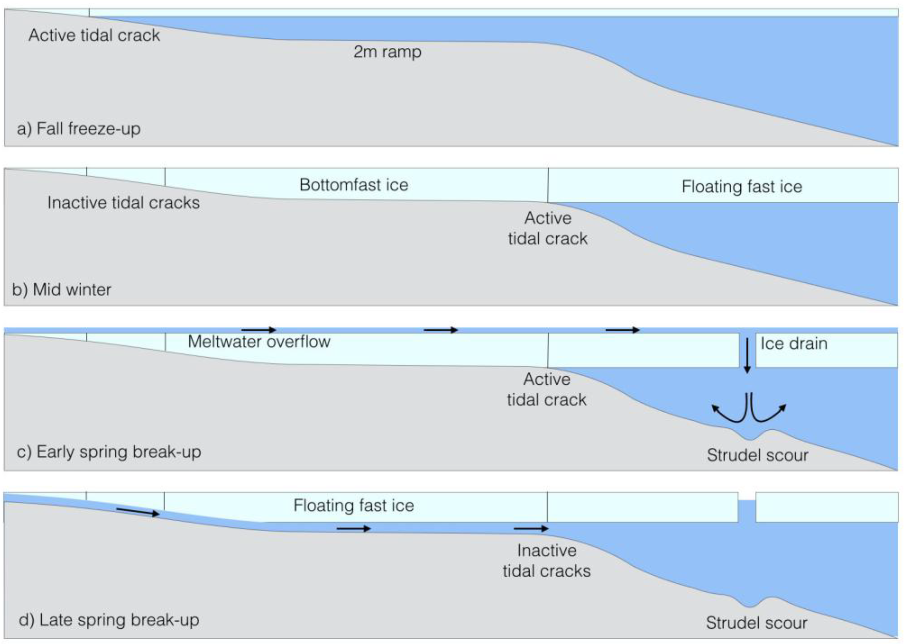
1.1. Evolution and Relevance of Bottomfast Sea Ice
1.2. Remote Sensing of Bottomfast Sea Ice
2. Materials and Methods
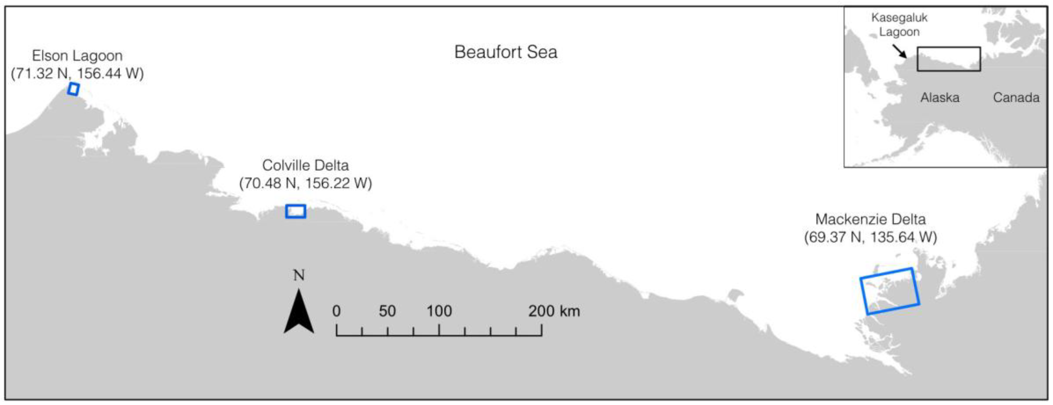
2.1. Study Area
2.2. Satellite Data
2.3. InSAR Processing and Concepts
2.4. In-Situ Data for Validation
2.5. Freezing-Degree-Day Model to Estimate Ice Thickness
3. Results
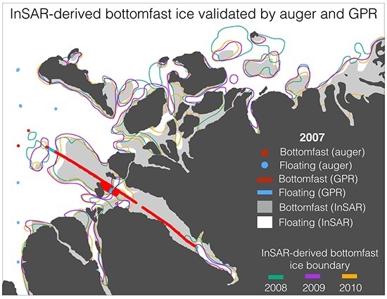
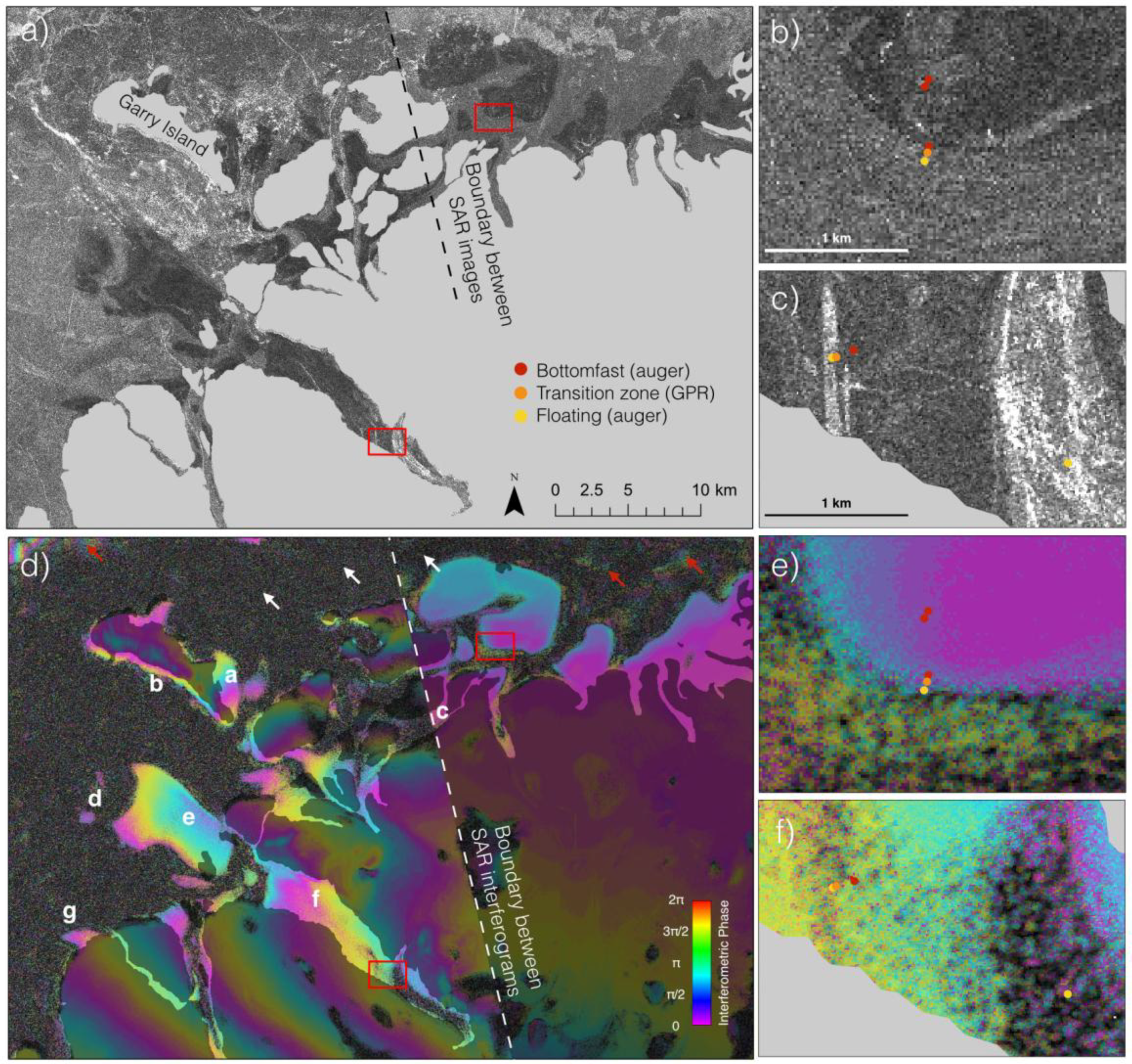
3.1. Mackenzie Delta
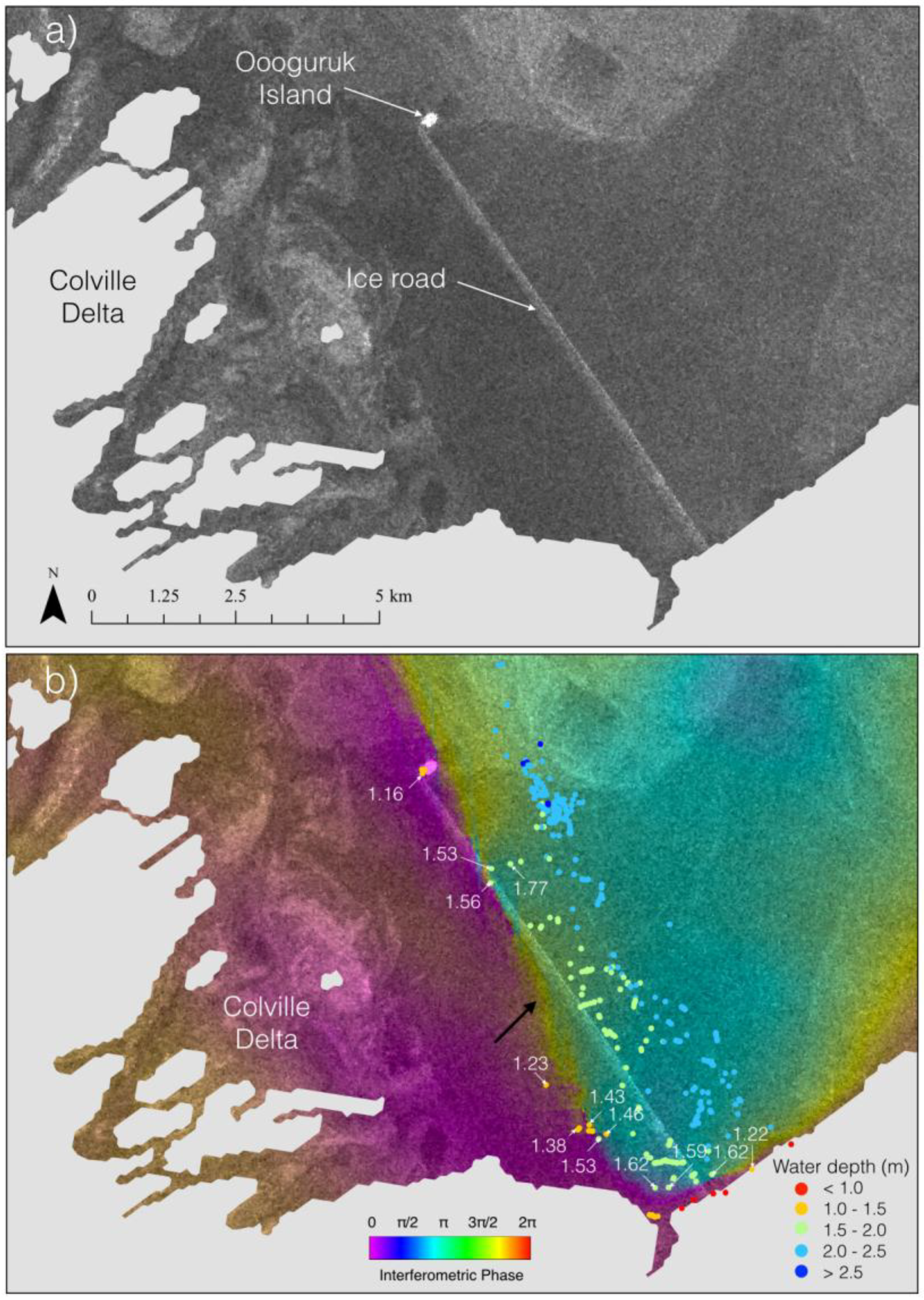
3.2. Colville Delta
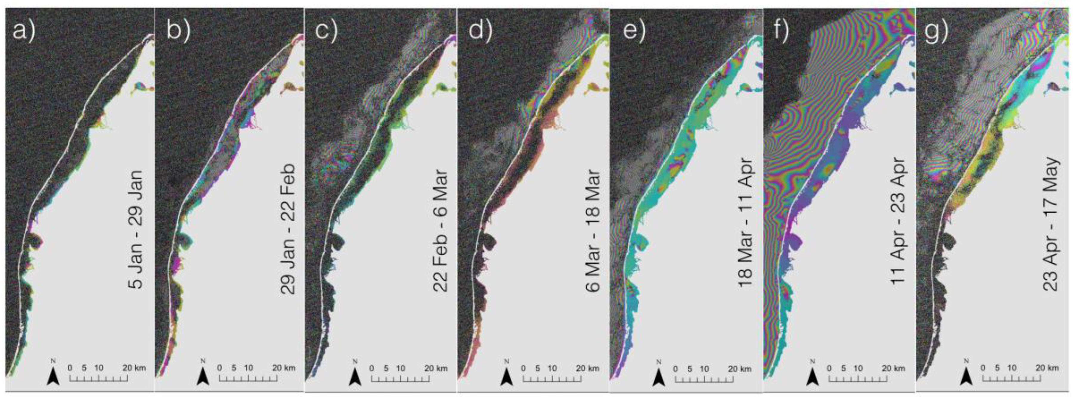
3.3. Elson Lagoon
4. Discussion
4.1. Delineation Constraints
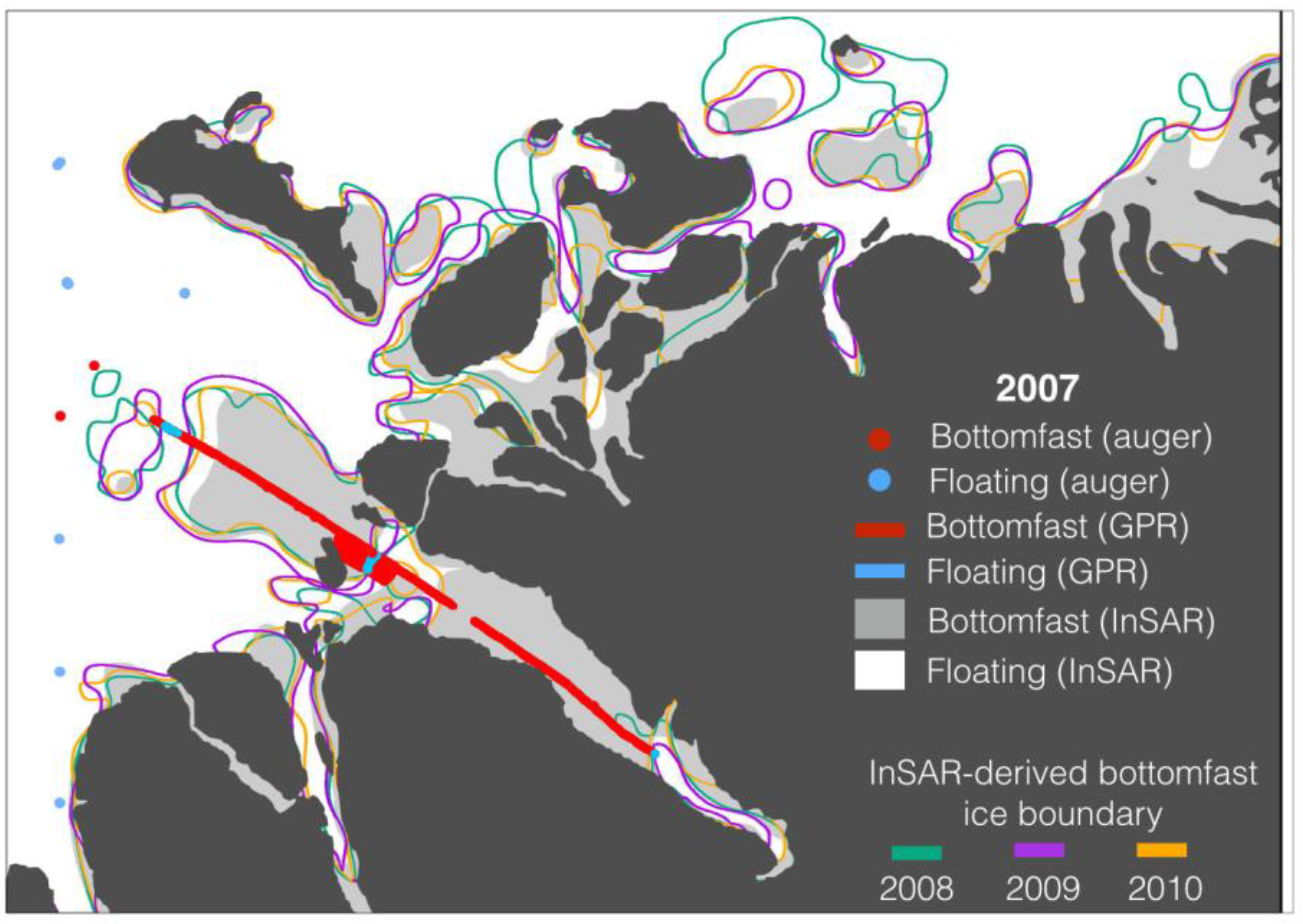
4.2. Tracking Bottomfast Ice on a Seasonal Scale
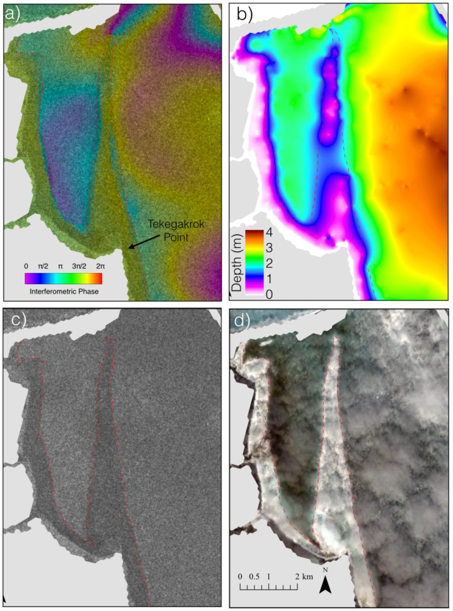
4.3. Detection of Bottomfast Sea Ice Using Optical Imagery
5. Conclusions
Author Contributions
Acknowledgments
Conflicts of Interest
References
- Eicken, H.; Lovecraft, A.L.; Druckenmiller, M.L. Sea-ice system services: A framework to help identify and meet information needs relevant for Arctic observing networks. Arctic 2009, 62, 119–136. [Google Scholar] [CrossRef]
- Stroeve, J.C.; Serreze, M.C.; Holland, M.M.; Kay, J.E.; Malanik, J.; Barrett, A.P. The Arctic’s rapidly shrinking sea ice cover: A research synthesis. Clim. Chang. 2012, 110, 1005–1027. [Google Scholar] [CrossRef]
- Comiso, J.C.; Hall, D.K. Climate trends in the Arctic as observed from space. Wiley Interdiscip. Rev. Clim. Chang. 2014, 5, 389–409. [Google Scholar] [CrossRef] [PubMed]
- Meier, W.N.; Hovelsrud, G.K.; Oort, B.E.; Key, J.R.; Kovacs, K.M.; Michel, C.; Haas, C.; Granskog, M.A.; Gerland, S.; Perovich, D.K. Arctic sea ice in transformation: A review of recent observed changes and impacts on biology and human activity. Rev. Geophys. 2014, 52, 185–217. [Google Scholar] [CrossRef]
- Mahoney, A.; Eicken, H.; Gaylord, A.G.; Gens, R. Landfast sea ice extent in the Chukchi and Beaufort Seas: The annual cycle and decadal variability. Cold Reg. Sci. Technol. 2014, 103, 41–56. [Google Scholar] [CrossRef]
- Selyuzhenok, V.; Krumpen, T.; Mahoney, A.; Janout, M.; Gerdes, R. Seasonal and interannual variability of fast ice extent in the southeastern Laptev Sea between 1999 and 2013. J. Geophys. Res. Oceans 2015, 120, 7791–7806. [Google Scholar] [CrossRef] [Green Version]
- Screen, J.A.; Simmonds, I. The central role of diminishing sea ice in recent Arctic temperature amplification. Nature 2010, 464, 1334–1337. [Google Scholar] [CrossRef] [PubMed] [Green Version]
- Post, E.; Bhatt, U.S.; Bitz, C.M.; Brodie, J.F.; Fulton, T.L.; Hebblewhite, M.; Kerby, J.; Kutz, S.J.; Stirling, I.; Walker, D.A. Ecological consequences of sea-ice decline. Science 2013, 341, 519–524. [Google Scholar] [CrossRef] [PubMed]
- Dammann, D.O. Arctic Sea Ice Trafficability—New Strategies for a Changing Icescape. Ph.D. Thesis, University of Alaska Fairbanks, Fairbanks, AK, USA, 2017. [Google Scholar]
- Solomon, S.M.; Taylor, A.E.; Stevens, C.W. Nearshore ground temperatures, seasonal ice bonding, and permafrost formation within the bottom-fast ice zone, Mackenzie Delta, NWT. In Proceedings of the Ninth International Conference on Permafrost, Fairbanks, AK, USA, 29 June–3 July 2008; University of Alaska Fairbanks: Fairbanks, AK, USA, 2008; pp. 1675–1680. [Google Scholar]
- Stevens, C.W.; Moorman, B.J.; Solomon, S.M. Interannual changes in seasonal ground freezing and near-surface heat flow beneath bottom-fast ice in the near-shore zone, Mackenzie Delta, NWT, Canada. Permafr. Periglac. Process. 2010, 21, 256–270. [Google Scholar] [CrossRef]
- Stevens, C.W.; Moorman, B.J.; Solomon, S.M. Detection of frozen and unfrozen interfaces with ground penetrating radar in the nearshore zone of the Mackenzie Delta, Canada. In Proceedings of the Ninth International Conference on Permafrost, Fairbanks, AK, USA, 29 June–3 July 2008; University of Alaska Fairbanks: Fairbanks, AK, USA, 2008; pp. 1711–1716. [Google Scholar]
- Stevens, C.W. Controls on Seasonal Ground Freezing and Permafrost in the Near-Shore Zone of the Mackenzie Delta, NWT, Canada. Ph.D. Thesis, University of Calgary, Calgary, AB, Canada, 2011. [Google Scholar]
- Eicken, H.; Dmitrenko, I.; Tyshko, K.; Darovskikh, A.; Dierking, W.; Blahak, U.; Groves, J.; Kassens, H. Zonation of the Laptev Sea landfast ice cover and its importance in a frozen estuary. Glob. Planet. Chang. 2005, 48, 55–83. [Google Scholar] [CrossRef]
- Are, F.; Reimnitz, E. An overview of the Lena River Delta setting: Geology, tectonics, geomorphology, and hydrology. J. Coast. Res. 2000, 1083–1093. [Google Scholar]
- Leidersdorf, C.B.; Hearon, G.E.; Vaudrey, K.D.; Swank, G. Strudel scour formation off Arctic river deltas. In Coastal Engineering 2006: (In 5 Volumes); World Scientific: Singapore, 2007; p. 5312. [Google Scholar]
- Dickins, D.; Hearon, G.; Morris, K.; Ambrosius, K.; Horowitz, W. Mapping sea ice overflood using remote sensing: Alaskan Beaufort Sea. Cold Reg. Sci. Technol. 2011, 65, 275–285. [Google Scholar] [CrossRef]
- Lanan, G.A.; Cowin, T.; Hazen, B.; Maguire, D.H.; Hall, J.D.; Perry, C.J. Oooguruk offshore Arctic flowline design and construction. In Proceedings of the Offshore Technology Conference, Houston, TX, USA, 5–8 May 2008. [Google Scholar]
- Hearon, G.; Dickins, D.; Ambrosius, K.K.M. Mapping Sea Ice Overflood Using Remote Sensing: Smith Bay to Camden Bay; Report Prepared by DF Dickins Associates, Minerals Management Service, Alaska OCS Region under Contract M06PC00034; Coastal Frontiers Corporation, Aerometric, and The Geophysical Institute; University of Alaska for US Department of Interior: Fairbanks, AK, USA, 2009. [Google Scholar]
- Reimnitz, E. Interaction of river discharge with sea ice in proximity of Arctic deltas: A review. Polarforschung 2002, 70, 123–134. [Google Scholar]
- Hirose, T.; Kapfer, M.; Bennett, J.; Cott, P.; Manson, G.; Solomon, S. Bottomfast ice mapping and the measurement of ice thickness on tundra lakes using c-band synthetic aperture radar remote sensing. J. Am. Water Resour. Assoc. 2008, 44, 285–292. [Google Scholar] [CrossRef]
- Hall, J. Oooguruk project offshore Alaska. Offshore Magazine, 1 August 2008; 68. [Google Scholar]
- Engram, M.; Arp, C.D.; Jones, B.M.; Ajadi, O.A.; Meyer, F.J. Analyzing floating and bedfast lake ice regimes across Arctic Alaska using 25 years of space-borne SAR imagery. Remote Sens. Environ. 2018, 209, 660–676. [Google Scholar] [CrossRef]
- Jeffries, M.; Morris, K.; Weeks, W.; Wakabayashi, H. Structural and stratigraphie features and ERS 1 synthetic aperture radar backscatter characteristics of ice growing on shallow lakes in NW Alaska, winter 1991–1992. J. Geophys. Res. Oceans 1994, 99, 22459–22471. [Google Scholar] [CrossRef]
- Hallikainen, M.; Winebrenner, D.P. The physical basis for sea ice remote sensing. Microw. Remote Sens. Sea Ice 1992, 29–46. [Google Scholar]
- Oggier, M.; Eicken, H. Tabulation of first-year sea-ice properties representative of the annual cycle as relevant to 2014 oil-in-ice experiments project. In Detection of Oil on-in-and-under Ice—Final Report 5.3; Pegau, W.S., Garron, J., Zabilansky, L., Eds.; Arctic Response Technology: London, UK, 2016; pp. 251–264. [Google Scholar]
- Yue, B.; Chamberland, J.; Mulvie, J. Bottom-fast ice delineation with polsar and insar techniques in the Mackenzie Delta Region, Northwest Territories, Canada. Can. J. Remote Sens. 2013, 39, 341–353. [Google Scholar] [CrossRef]
- Dammann, D.O.; Eicken, H.; Meyer, F.; Mahoney, A. Assessing small-scale deformation and stability of landfast sea ice on seasonal timescales through l-band SAR interferometry and inverse modeling. Remote Sens. Environ. 2016, 187, 492–504. [Google Scholar] [CrossRef]
- Berg, A.; Dammert, P.; Eriksson, L.E. X-band interferometric SAR observations of Baltic fast ice. IEEE Trans. Geosci. Remote Sens. 2015, 53, 1248–1256. [Google Scholar] [CrossRef]
- Li, S.; Shapiro, L.; McNutt, L.; Feffers, A. Application of satellite radar interferometry to the detection of sea ice deformation. J. Remote Sens. Soc. Jpn. 1996, 16, 67–77. [Google Scholar]
- Meyer, F.J.; Mahoney, A.R.; Eicken, H.; Denny, C.L.; Druckenmiller, H.C.; Hendricks, S. Mapping Arctic landfast ice extent using l-band synthetic aperture radar interferometry. Remote Sens. Environ. 2011, 115, 3029–3043. [Google Scholar] [CrossRef]
- Zebker, H.A.; Villasenor, J. Decorrelation in interferometric radar echoes. IEEE Trans. Geosci. Remote Sens. 1992, 30, 950–959. [Google Scholar] [CrossRef]
- Mikhailova, M. Hydrological processes at an Arctic river mouth: Case study of the Colville River, Alaska, USA. Water Resour. 2009, 36, 26–42. [Google Scholar] [CrossRef]
- Ferretti, A.; Monti-Guarnieri, A.; Prati, C.; Rocca, F.; Massonet, D. Insar principles-guidelines for SAR interferometry processing and interpretation. ESA Publ. 2007, TM-19, 40. [Google Scholar]
- Bamler, R.; Hartl, P. Synthetic aperture radar interferometry. Inverse Probl. 1998, 14, R1. [Google Scholar] [CrossRef]
- Haas, C.; Druckenmiller, M. Ice thickness and roughness measurements. In Field Techniques for Sea Ice Research; Eicken, H., Gradinger, R., Salganek, M., Shirasawa, K., Perovich, D., Leppäranta, M., Eds.; University of Alaska Press: Fairbanks, AK, USA, 2009; pp. 49–116. [Google Scholar]
- Stevens, C.W.; Moorman, B.J.; Solomon, S.M.; Hugenholtz, C.H. Mapping subsurface conditions within the near-shore zone of an Arctic delta using ground penetrating radar. Cold. Reg. Sci. Technol. 2009, 56, 30–38. [Google Scholar] [CrossRef]
- Dammann, D.O.; Eicken, H.; Mahoney, A.; Meyer, F.; Betcher, S. Assessing sea ice trafficability in a changing Arctic. Arctic 2018, 71, 59–75. [Google Scholar] [CrossRef]
- Anderson, D.L. Growth rate of sea ice. J. Glaciol. 1961, 3, 1170–1172. [Google Scholar] [CrossRef]
- Petrich, C.; Eicken, H. Growth, structure and properties of sea ice. In Sea Ice; Thomas, D.N., Dieckmann, G.S., Eds.; Wiley-Blackwell: Oxford, UK, 2010; Volume 2, pp. 23–77. [Google Scholar]
- Walker, H. Spring discharge of an Arctic river determined from salinity measurements beneath sea ice. Water Resour. Res. 1973, 9, 474–480. [Google Scholar] [CrossRef]
- Tweedie, C.E.; Escarzaga, S.; Manley, W.F.; Tarin, G.; Gaylord, A. Interpolated Bathymetric Surface for the Elson Lagoon, Barrow, Northern Alaska, 2015. Barrow Area Information Database (BAID), 2016. Digital Media. Available online: http://barrowmapped.org (accessed on 7 May 2018).
- Stierle, A.P.; Eicken, H. Sediment inclusions in Alaskan coastal sea ice: Spatial distribution, interannual variability, and entrainment requirements. Arct. Antarct. Alp. Res. 2002, 34, 465–476. [Google Scholar] [CrossRef]
- Wessel, P.; Smith, W.H. A global, self-consistent, hierarchical, high-resolution shoreline database. J. Geophys. Res. Solid Earth 1996, 101, 8741–8743. [Google Scholar] [CrossRef]
- Frost, K.; Lowry, L.; Carroll, G. Use of Kasegaluk Lagoon, Chukchi Sea, Alaska, by Marine Birds and Mammals, III: Marine Mammals; Minerals Management Service, U.S. Department of Interior Anchorage, Alaska: Anchorage, AK, USA, 1992; p. 627.
- Overduin, P.P.; Westermann, S.; Yoshikawa, K.; Haberlau, T.; Romanovsky, V.; Wetterich, S. Geoelectric observations of the degradation of nearshore submarine permafrost at Barrow (Alaskan Beaufort Sea). J. Geophys. Res. Earth Surf. 2012, 117. [Google Scholar] [CrossRef]


| Area | Satellite | Orbit | Frame | Date | BT (d) | Θ |
|---|---|---|---|---|---|---|
| Mackenzie | PALSAR | 05021, 05692 | 1390 | 3 January–18 February 2007 | 46 | 36.6–40.9 |
| Mackenzie | PALSAR | 10389, 11060 | 1390 | 6 January–21 February 2008 | 45 | 36.6–40.9 |
| Mackenzie | PALSAR | 15757, 16428 | 1390 | 8 January–23 February 2009 | 46 | 36.6–40.9 |
| Mackenzie | PALSAR | 21125, 21796 | 1390 | 11 January–26 February 2010 | 45 | 36.6–40.9 |
| Mackenzie | PALSAR | 21971, 22642 | 1390 | 10 March–25 April 2010 | 45 | 36.6–40.9 |
| Colville Delta | Sentinel-1 | 5195, 5370 | 230 | 17–29 April 2017 | 12 | 30.0–47.3 |
| Elson Lagoon | Sentinel-1 | 5312, 5487 | 230 | 25 April–7 May 2017 | 12 | 30.0–47.3 |
| Kasegaluk | Sentinel-1 | 3708, 4058 | 226 | 5–29 January2017 | 24 | 30.0–47.4 |
| Kasegaluk | Sentinel-1 | 4058, 4408 | 226 | 29 January–22 February 2017 | 24 | 30.0–47.4 |
| Kasegaluk | Sentinel-1 | 4408, 4583 | 226 | 22 February–6 March 2017 | 12 | 30.0–47.4 |
| Kasegaluk | Sentinel-1 | 4583, 4758 | 226 | 6–18 March 2017 | 12 | 30.0–47.4 |
| Kasegaluk | Sentinel-1 | 4758, 5108 | 226 | 18 March–11 April 2017 | 24 | 30.0–47.4 |
| Kasegaluk | Sentinel-1 | 5108, 5283 | 226 | 11–23 April 2017 | 12 | 30.0–47.4 |
| Kasegaluk | Sentinel-1 | 5283, 5633 | 226 | 23 April–17 May 2017 | 24 | 30.0–47.4 |
© 2018 by the authors. Licensee MDPI, Basel, Switzerland. This article is an open access article distributed under the terms and conditions of the Creative Commons Attribution (CC BY) license (http://creativecommons.org/licenses/by/4.0/).
Share and Cite
Dammann, D.O.; Eriksson, L.E.B.; Mahoney, A.R.; Stevens, C.W.; Van der Sanden, J.; Eicken, H.; Meyer, F.J.; Tweedie, C.E. Mapping Arctic Bottomfast Sea Ice Using SAR Interferometry. Remote Sens. 2018, 10, 720. https://doi.org/10.3390/rs10050720
Dammann DO, Eriksson LEB, Mahoney AR, Stevens CW, Van der Sanden J, Eicken H, Meyer FJ, Tweedie CE. Mapping Arctic Bottomfast Sea Ice Using SAR Interferometry. Remote Sensing. 2018; 10(5):720. https://doi.org/10.3390/rs10050720
Chicago/Turabian StyleDammann, Dyre O., Leif E. B. Eriksson, Andrew R. Mahoney, Christopher W. Stevens, Joost Van der Sanden, Hajo Eicken, Franz J. Meyer, and Craig E. Tweedie. 2018. "Mapping Arctic Bottomfast Sea Ice Using SAR Interferometry" Remote Sensing 10, no. 5: 720. https://doi.org/10.3390/rs10050720