Hyperspectral Imagery Classification Based on Semi-Supervised Broad Learning System


1
School of Information and Control Engineering, China University of Mining and Technology, Xuzhou 221116, China
2
Department of Computer and Information Science, Faculty of Science and Technology, University of Macau, Macau 99999, China; also with the State Key Laboratory of Management and Control for Complex Systems, Institute of Automation, Chinese Academy of Sciences, Beijing 100080, China
*
Author to whom correspondence should be addressed.
Remote Sens. 2018, 10(5), 685; https://doi.org/10.3390/rs10050685
Submission received: 26 March 2018
/
Revised: 18 April 2018
/
Accepted: 26 April 2018
/
Published: 28 April 2018
(This article belongs to the Section Remote Sensing Image Processing)
Abstract
:Recently, deep learning-based methods have drawn increasing attention in hyperspectral imagery (HSI) classification, due to their strong nonlinear mapping capability. However, these methods suffer from a time-consuming training process because of many network parameters. In this paper, the concept of broad learning is introduced into HSI classification. Firstly, to make full use of abundant spectral and spatial information of hyperspectral imagery, hierarchical guidance filtering is performing on the original HSI to get its spectral-spatial representation. Then, the class-probability structure is incorporated into the broad learning model to obtain a semi-supervised broad learning version, so that limited labeled samples and many unlabeled samples can be utilized simultaneously. Finally, the connecting weights of broad structure can be easily computed through the ridge regression approximation. Experimental results on three popular hyperspectral imagery datasets demonstrate that the proposed method can achieve better performance than deep learning-based methods and conventional classifiers.
1. Introduction
Hyperspectral imagery (HSI) captured by hyperspectral sensors has high spectral and spatial resolution, thus has a strong capability to distinguish surface objects [1]. HSI has been widely applied in many fields including agricultural monitoring [2], environment analysis and prediction [3], and climate monitoring [4]. HSI classification is a common task in these applications, i.e., to assign a class label of surface object to every HSI pixel by using a small number of training samples.
In recent years, many methods have been proposed to address HSI classification. The K-nearest neighborhood (KNN) [5] determines the class of testing sample by calculating the Euclidean distance between testing and training samples. Support vector machine (SVM) [6,7] projects samples to a high-dimensional space by kernel functions and distinguishes sample classes by learning a classification hyperplane, which achieves satisfactory performance in the small-sample classification tasks. Extreme learning machine (ELM) [8,9] is a single hidden-layer neural network which has the following characteristics: (1) the connecting weights between input-layer and hidden-layer neurons are randomly assigned and do not need to be adjusted during the learning process; and (2) the connecting weights between hidden-layer and output-layer neurons can be calculated via the least square method. Therefore, the computational efficiency of ELM is high.
Recently, deep learning (DL) is found to be able to automatically learn representative features from data via stacking multi-layer nonlinear units [10,11], making successful application on HSI analysis. Chen et al. [12] firstly introduced DL into HSI classification, and directly deemed spectral and spatial information as inputs of stacked autoencoder (SAE). Afterwards, Tao et al. [13] added sparse constraints on SAE and Chen et al. [14] introduced the deep belief network. The unsupervised CNN was designed by Romero et al. [15]. By layer-wise training approach, the unsupervised sparse features of HSI are learned. Compared with unsupervised CNN, supervised CNN can extract features that are more helpful on classification. A CNN with pixel-pair features (CNN-PPF) was proposed by Li et al. [16]. By comparing the classes of a couple of samples, new training samples are obtained, which highly outnumbered the original, and thus ensures a vast number of parameter learning in CNN. In terms of limited labeled samples as well as dimensionality disaster problem, Santara et al. [17] proposed BASS-Net. Compared with conventional CNN, BASS-Net has fewer parameters and needs fewer training samples. By simplifying the training process, Pan et al. [18] introduced PCANet to realize HSI classification and further the NSSNet for more complex nonlinear mapping by using kernel PCA (KPCA) instead of PCA due to insufficient expression of nonlinearity from PCANet. In later study, Pan et al. [19] further proposed R-VCANet comprehensively using rolling guidance filter (RGF) and vertex component analysis network (VCANet). Compared with conventional CNN, R-VCANet has a simpler structure and fewer network parameters, which demand fewer labeled training samples. Meanwhile, the fully utilized spatial information of HSI makes the extracted features from network more discriminative, thus achieving higher classification accuracy. Several experiments on hyperspectral datasets demonstrated that the classification accuracy of R-VCANet is higher than other deep learning methods such as R-PCANet and NSSNet.
However, DL methods require complicated structural adjustment and a vast computation of network training. Aiming at such problems, Chen and Liu [20] proposed a novel broad learning system (BLS) to offer an optional learning approach. The approach is based on the random vector functional link neural network (RVFLNN) [21,22]. First, the original data are mapped via random weights as mapped features (MF) and stored in feature nodes. Next, MF is similarly mapped via random weights to obtain enhancement nodes (EN) for broad expansion. Finally, the normalized optimization of l2-norm is solved by ridge regression approximation to get ultimate network weights. Compared with DL, BLS has the following advantages: (1) BLS is merely composed of three parts while the deep learning requires deep structure that is stacked by multiple nonlinear units. Therefore, BLS has a simpler structure. (2) BLS solves the network weights with ridge regression while DL adopts gradient descent. When the weights are not well initialized, DL requires more iterations. Therefore, the training process of BLS is simpler and faster. (3) The connecting weights from input data to MF and from MF to EN in BLS are randomly generated and the trainable parameters merely include the connecting weights from MF and EN to output nodes. Therefore, compared with DL, BLS generally needs less network parameter training and hence fewer labeled training samples. In the tasks of HSI classification, there exactly exists such a problem of limited numbers of labeled samples. Therefore, BLS might be better suited to HSI classification than DL. However, BLS belongs to supervised classification method while the unlabeled samples are huge in number. To fully make use of this part of information, it is necessary to investigate semi-supervised BLS.
Semi-supervised learning (SSL) methods have attracted much research attention recently due to its capability of full use of both vast numbers of unlabeled samples and the limited numbers of labeled samples. Plenty of graph-based SSL methods have been successively proposed, such as the adjacency structure of graph is constructed by KNN or ε-ball neighborhood, which further determines weight matrices by Gaussian kernel [23,24], non-negative local linear reconstruction coefficients [25], etc. However, SSL methods based on conventional graph have the following disadvantages: (1) the algorithm performance is heavily influenced by graphs to be constructed; and (2) higher sensitivity occurs in terms of neighboring parameters. Considering these problems, SSL methods based on sparse graph were successively proposed. The nonnegative low-rank and sparse graph proposed by Zhuang et al. [26] can capture both the global mixture of subspaces structure (by the low-rankness) and the locally linear structure (by the sparseness) of data, hence it is both generative and discriminative. Morsier et al. [27] presented a kernel low-rank and sparse graph, which was based on sample proximities in reproducing kernel Hilbert spaces and expressed sample relationships under sparse and low-rank constraints. However, data class structure is not considered in the above methods. Considering this, Shao, et al. [28] presented a class-probability (CP) structure, which can express the relation between each sample and each class via a class-probability matrix.
In summary, a HSI classification method is proposed based on a semi-supervised BLS (SBLS). The main contributions of this paper include: (1) To our knowledge, this is the first trial where BLS is applied in HSI classification tasks. The proposed SBLS can get higher HSI classification accuracy and faster training speed. (2) The class-probability structure is introduced into BLS for an extended semi-supervised BLS to make use of limited numbers of labeled samples as well as vast unlabeled samples.
2. HSI Classification Based On SBLS
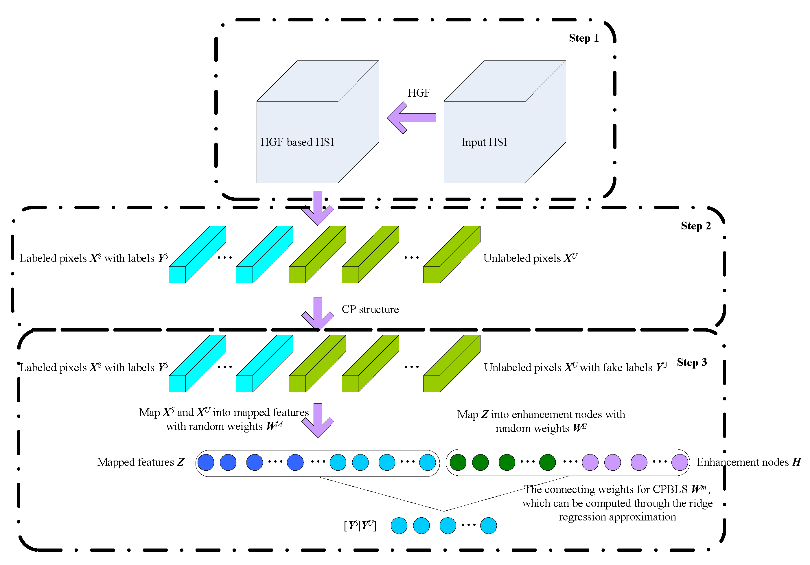
The flowchart of HSI classification based on SBLS is shown in Figure 1 and includes three steps: (1) the original HSI data are processed by hierarchical guidance filtering (HGF) to get the spectral-spatial expression of HSI; (2) the pseudo labels of unlabeled samples are obtained via CP structure; and (3) SBLS is trained by labeled samples and corresponding labels, as well as unlabeled samples and corresponding pseudo labels.
2.1. Hierarchical Guidance Filtering
The first step of SBLS is to get the HGF representation of HSI, shown as Step 1 in Figure 1. The original hyperspectral images are expressed in the form of 3D tensor. If vectorization is expressed by a tensor, not only is the data dimension greatly increased, but the inherent data structure is also destroyed. Pan et al. [29] proposed a spectral-spatial expression of HSI data by using HGF. As one of the edge-preserving filtering methods, HGF can remove noise and small details while preserving the overall structure of the image, thus can map the original HSI data into a feature subspace having more abundant feature expression. In terms of the superiority of HGF, the original HSI is processed by HGF to get the spectral-spatial expression of HSI.
As an extension of guided filtering and rolling guidance filtering, HGF can generate a series of joint spectral-spatial features. HGF minimizes the following energy function:
where and are linear coefficients based on the input HSI data and the guidance image , is the window around pixel k with size , is the window radius, is one of a pixel in , denotes the p-th band, and ε is the controlling parameter. Larger ε will lead smoother output. Equation (1) is a ridge regression, and can be solved by:
where and are the mean and standard variance of , respectively; is the mean of in ; and is the number of pixels in . More details can be found in [29]. HGF is a kind of preprocessing trick, and a similar strategy is also used in [19,29].
2.2. Class-Probability Structure
The second step of SBLS is to obtain the pseudo labels of unlabeled samples via CP structure, shown as Step 2 in Figure 1. The labeled samples via HGF expression and corresponding labels are given, where is the number of labeled samples, m is the number of dimensionality, c is the number of classes, is a binary number and if the i-th sample belongs to j-th class, , or else . Given the unlabeled samples via HGF expression, where means the number of unlabeled samples, the overall number of samples is . Hence, the similarity between the labeled and unlabeled samples can be expressed by the following:
where is the sparsity coefficient. Equation (3) can be solved with alternating direction methods of multipliers with adaptive penalty (ADMAP). More details can be referred to in [28]. The class-probability vector of xi is written as:
where , and means the probability that the i-th sample belongs to the c-th class. Regarding the unlabeled samples, it is feasible to get the class-probability matrix via label propagation for a given sample. Regarding the labeled samples, the class-probability matrix is defined. Therefore, the probability that the i-th and the j-th samples belong to an identical class is written as:
As a further step, P can be expressed as , where means the probability that the labeled samples have the same class while means the probability that the unlabeled samples have the same class. and represent the probabilities that the unlabeled and labeled samples have the same class, respectively. Finding the index of maximum probability per row in , can obtain the labeled sample that is most similar to each unlabeled one as well as the pseudo label of the unlabeled samples. The calculation principle is as follows:
2.3. SBLS
The third step of SBLS is to train the SBLS model and get the predictive labels of unlabeled samples, shown as Step 3 in Figure 1. BLS is proposed based on RVFLNN, including three parts: mapped features (which are the mapping from inputs), enhancement nodes (which are the mapping from mapped features), and output labels (which are the joint mapping from mapped features and enhancement nodes). The learning parameter is , which can be fast and approximately obtained by ridge regression. However, the BLS model belongs to the supervised method and cannot utilize vast numbers of commonly unlabeled samples in HSI. Hence, for better adaption of BLS into HSI classification, it is necessary to investigate semi-supervised BLS. Here, CP is introduced into BLS and SBLS is proposed to realize the semi-supervision classification of HSI.
HSI samples generally expressed by HGF are given, as well as labels and that are obtained by the class-probability structure. In terms of SBLS, the input is first mapped to “mapped features” via the random weight and bias , which is:
where is the number of groups of MF. is a nonlinear function, and different functions can be chosen for different groups of MF. Here, linear mapping is used in all MF for simplicity, which means . To have better features, WM is usually fine-tuned by linear sparse auto encoder.
After obtaining the MF, , the expansion of SBLS can be realized by mapping the features of MF to EN with random weights and bias
where is the number of ENs. Further, the SBLS model is expressed as:
where are the connecting weights from MF and EN to output nodes. It can be solved the following problem:
where denotes the further constraints on the sum of the Wm. The solution of Equation (8) can be solved by ridge regression:
If , Equation (8) degenerates into the least square problem. On the other hand, if , the solution is heavily constrained and tends to 0. Thus, we set here, such as . By giving an approximation to the Moore–Penrose generalized inverse of , Equation (8) can be written as:
Specifically, we have:
Finally, the predictive labels can be obtained by
In summary, the algorithm steps of HSI classification based on SBLS is shown in Table 1.
3. Experiments and Analysis
3.1. HSI Datasets
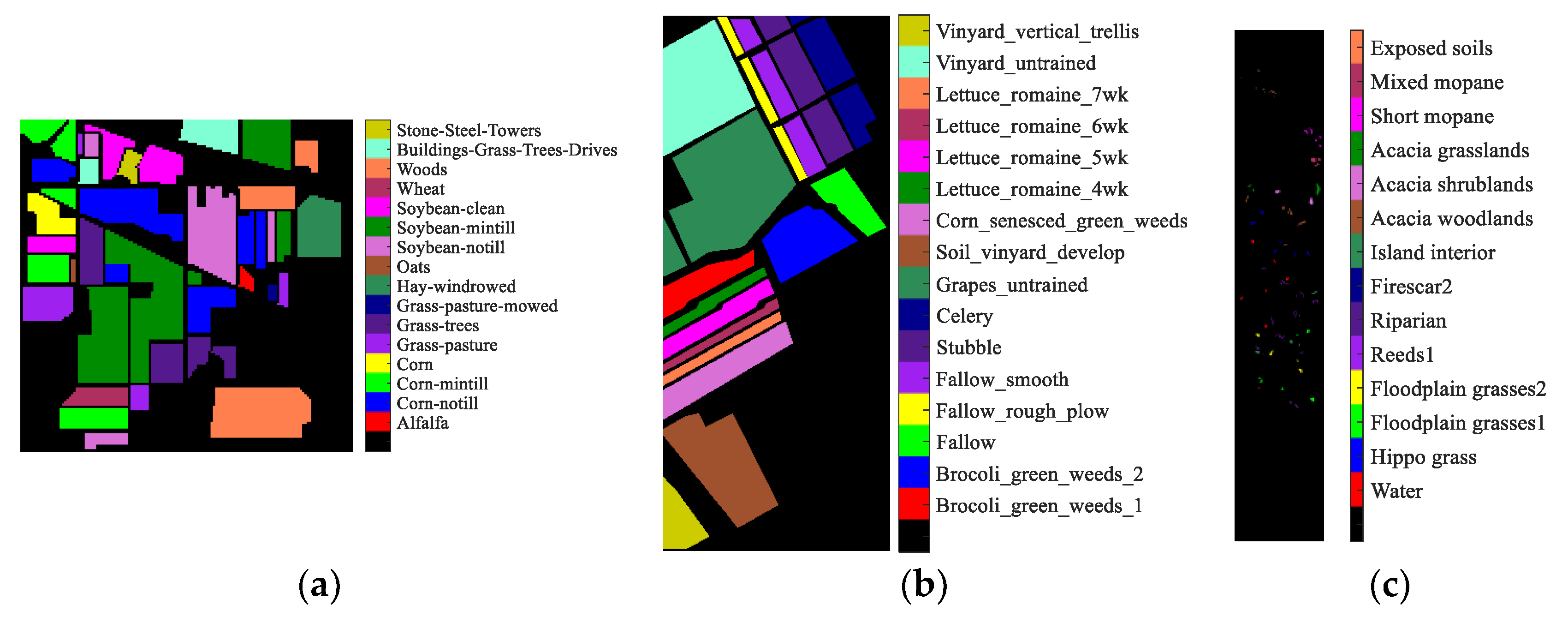
In this section, three real HSI datasets, i.e. Indian Pines, Salinas and Botswana, are used to evaluate the accuracy and efficiency of the proposed SBLS method. Figure 2 shows the ground truth maps of the three HSI datasets. For the three HSI datasets, 20 samples are randomly selected from different surface objects as labeled (training) samples, with the remaining as unlabeled (testing) samples.
(1) For supervised classification methods, only the labeled samples are used to train the classifier and the trained classifier is used to predict the labels of unlabeled samples.
(2) For semi-supervised classification methods, all labeled and unlabeled samples are used to train the classifier. In addition, since the total size of Salinas dataset is large, only part of labeled samples participates in the classifier training.
(3) Since the total size of surface object “Oats” in Indian Pines dataset is small, the size of labeled samples (denoted by s.l.s.) equals that of unlabeled samples (denoted by s.u.s.). The detailed sample settings for different HSI datasets are shown in Table 2.
3.2. Comparative Experiments
To evaluate the performance of the proposed SBLS on HSI classification, we investigate the following nine methods for comparison.
(1) Traditional classifiers include SVM [6], ELM [8], and SPELM [9]. Since only the linear feature mapping is used in BLS and SBLS, the linear kernel function is used in SVM and ELM in our experiments. The hyper parameters of SVM and ELM are selected through five-fold cross validation, and the penalty factor of SVM and the regularization coefficient of ELM and SPELM are selected from {1, 10, 100, 1000}. In addition, HSI data after HGF preprocessing were taken as the input of SVM, ELM, and SPELM for fair comparison. The number of trails of SPELM is set as 50.
(2) Semi-supervised graph-based classification method is SSG [23]. The width of Gaussian and regularization parameter are selected from {10−5, 10−4, …, 105}.
(3) Deep learning-based methods include CNN-PPF [16], BASS-Net [17], and R-VCANet [19]. The network configurations of CNN-PPF, BASS-Net, and R-VCANet refer to corresponding articles, respectively.
(4) Spectral-spatial classification method is HiFi-We [29].
(5) BLS [20], where HSI data after HGF preprocessing were taken as the input of BLS.
The proposed SBLS and nine comparative methods are used on the three HSI datasets for classification. Related experiments about CNN-PPF and BASS-Net are tested on Theano and Torch platforms with GPU GTX 980. Other experiments are performed in MATLAB R2014a using a computer with a 3.60 GHz Intel Core i7-4790 CPU and 16 GB of RAM. Each experiment is conducted five times to get the average value for stochastic. Table 3, Table 4 and Table 5, respectively, show the comparison of classification performance on different datasets, where five performance indexes are considered: the accuracy on each surface object (%), average accuracy (AA, %), overall accuracy (OA, %), Kappa coefficient, and consumed time (t, s) for classifier training and testing sample classification.
(1) The AA, OA, and Kappa coefficient of SBLS on the three datasets are the highest. This is because the CP structure is introduced into SBLS, which can make use of vast unlabeled samples compared with BLS.
(2) ELM has the shortest period of consumed time, followed by SVM. Besides SVM and ELM, BLS has the shortest consumed time. This is because the BLS network parameters can be directly solved by the generalized inverse and BLS has simple network.
(3) CNN-PPF, BASS-Net, and R-VCANET have longer consumed time. This is because these methods belong to deep learning. For BASS-Net, a high number of iteration steps are needed when the network parameters are updated based on the gradient descent. For CNN-PPF, to ensure the training of the CNN with many layers, the training samples are expanded greatly in number and, therefore, it has longer training time. For R-VCANet, its testing process is time-consuming due to the high dimensions of extracted features per layer.
(4) Compared with BLS, SBLS has longer period of consumed time. This is because the correlation computation between samples in CP structure consumes much time.
3.3. Parameter Analysis
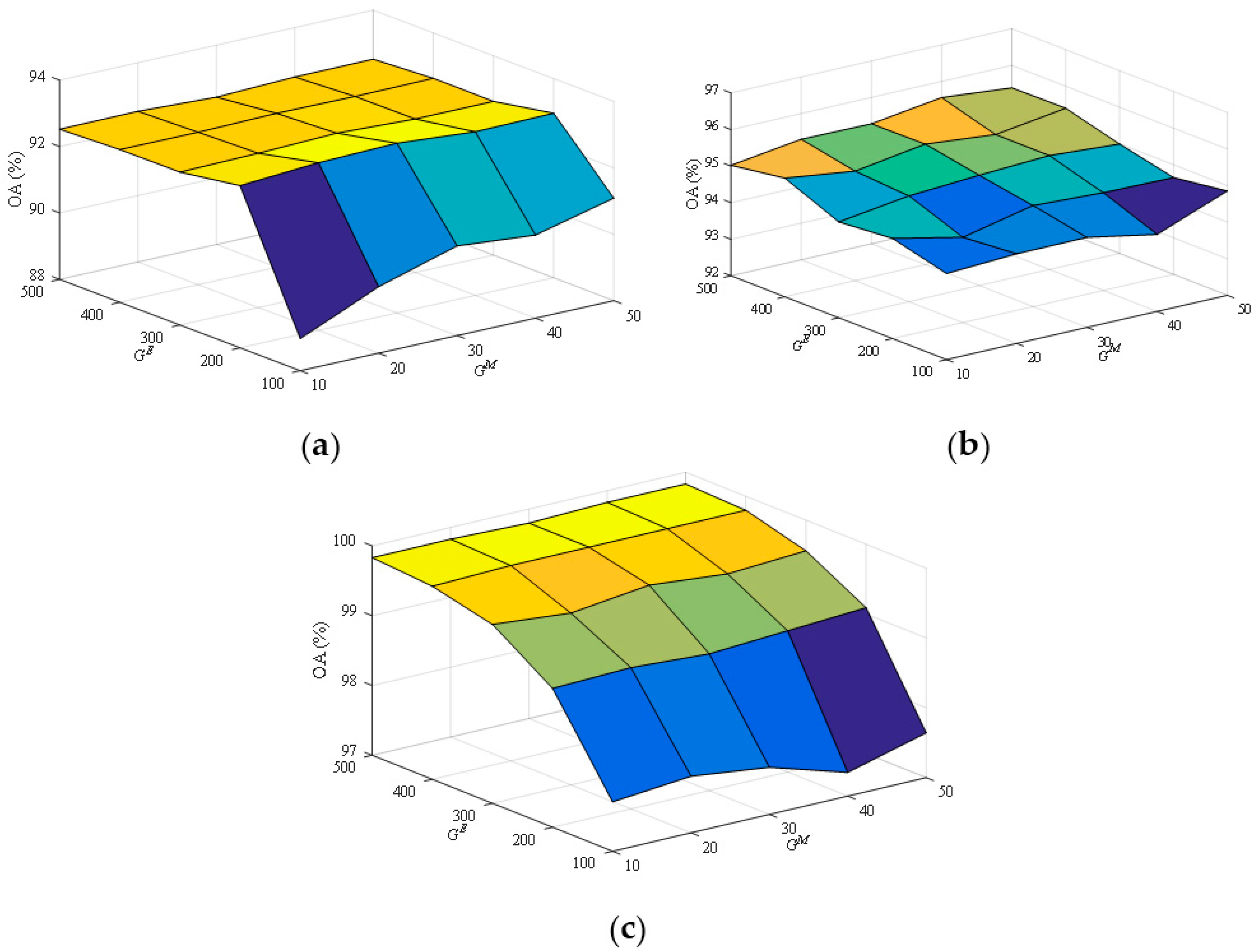
The adjustable parameters in SBLS include: MF group number, and number of MF nodes per group. Let MF group number equal to number of nodes per MF, which is set as . The number of EN nodes is set as . The relation between OA and or of SBLS on the three datasets is shown in Figure 5. It is demonstrated that:
(1) With increase of and , the OA on each of the three datasets takes on the tendency of rising up first and then dropping down. This is because the expression ability of SBLS increases gradually and saturates with increase of and .
(2) The excessively low and will lead to the OA decrease while the excessively high and will lead to additional computation. Therefore, and are, respectively, selected as 30–100, 40–400 and 20–500 in terms of the three datasets.
4. Discussion
The experimental results show the following:
(1) From the aspect of classification accuracy, our proposed method, SBLS, achieves the highest performance. There are two main reasons. First, BLS helps us to get a more accurate mapping between input HSI and labels by utilizing a small amount of labeled samples. Then, by exploring the relationship between each sample and each class with class-probability structure, we can obtain the most similar labeled samples to each unlabeled one. Furthermore, the pseudo labels of unlabeled samples can be given, and both the labeled and unlabeled samples can be utilized.
(2) From the aspect of consumed time, compared with deep learning-based methods, BLS and SBLS consumed less time. The reasons can be summarized as two aspects. On the one hand, the architectures of two broad learning-based methods only contain three parts (MF, EN and output layer), while the deep learning-based methods are built with many layers. On the other hand, the trainable parameters of broad learning are less than deep learning, and can be easily solved with ridge regression. Compared with BLS, SBLS is more time-consuming because of the utilizing of more samples and the extra computation for obtaining the class-probability matrix.
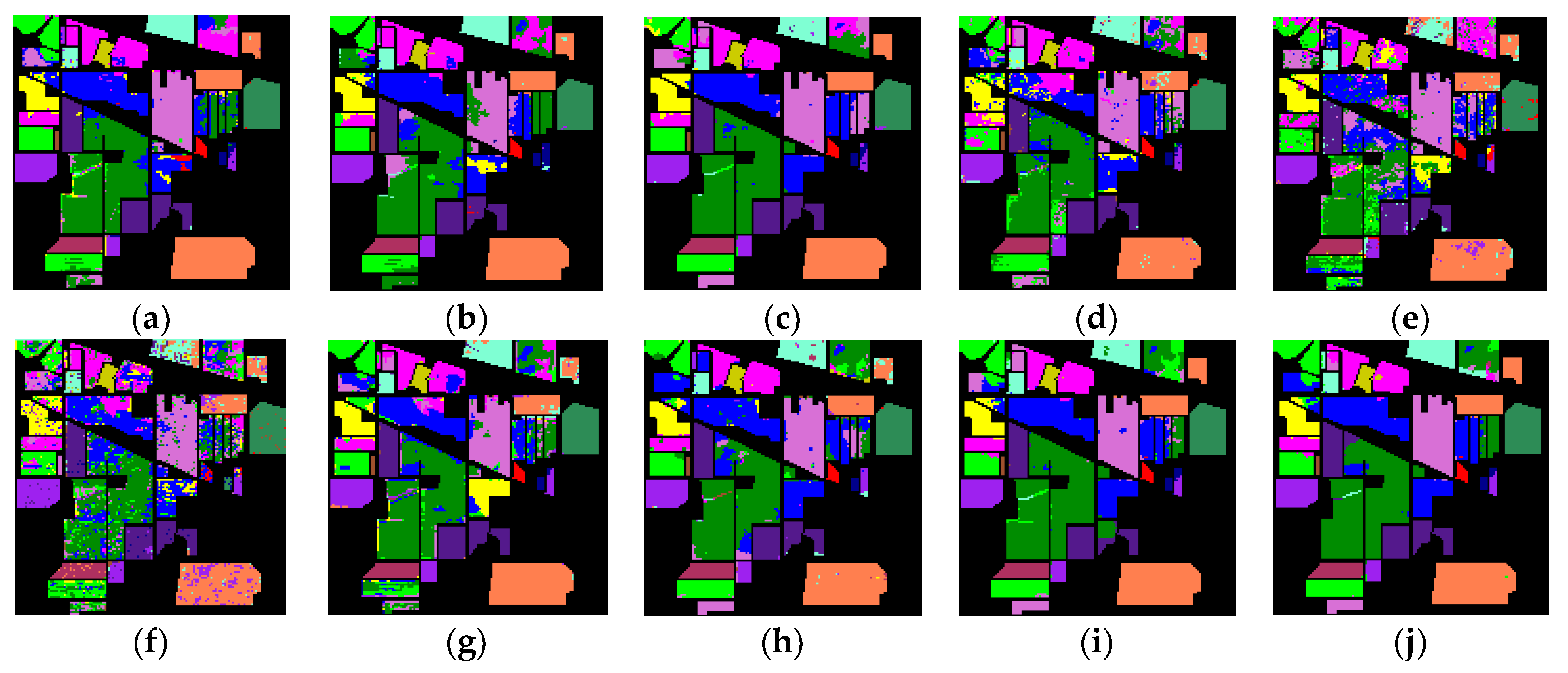
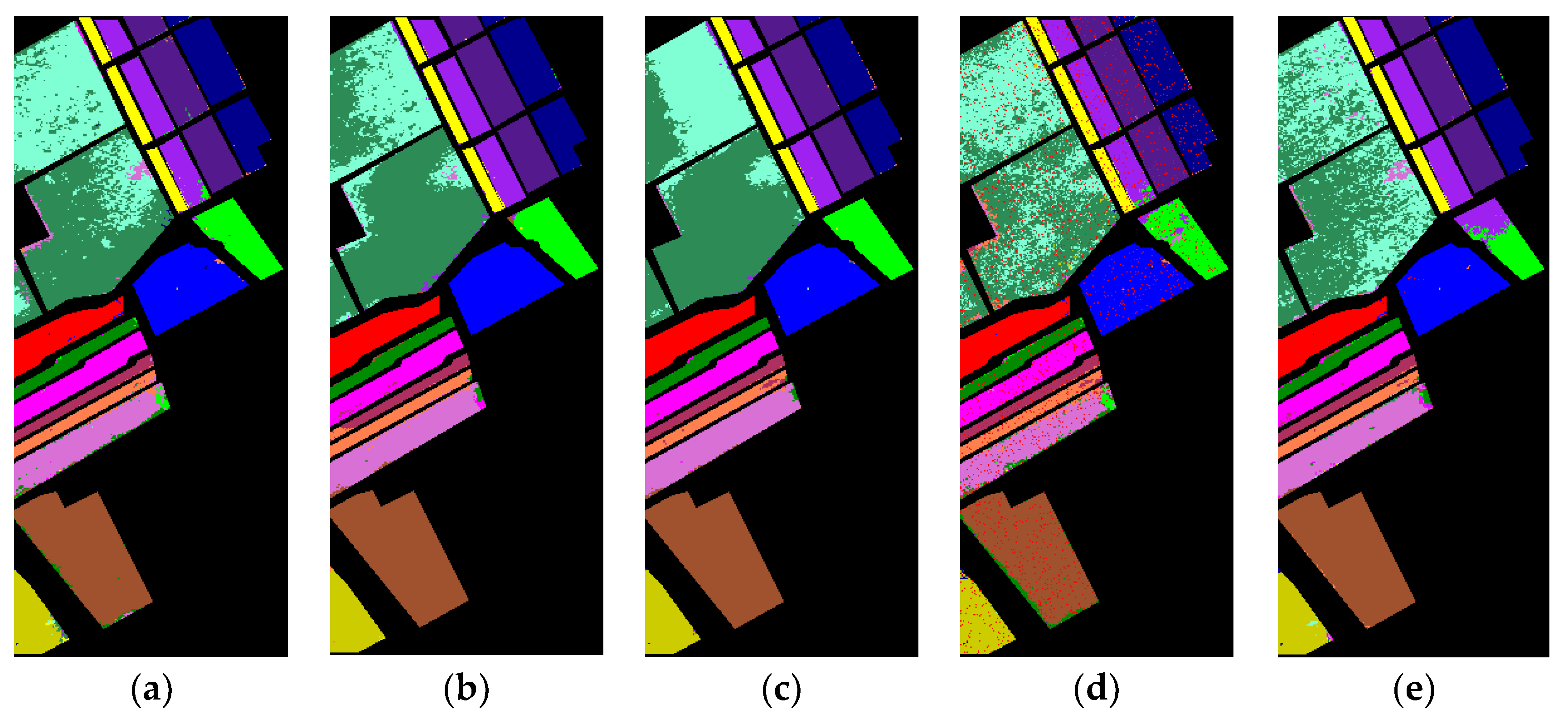
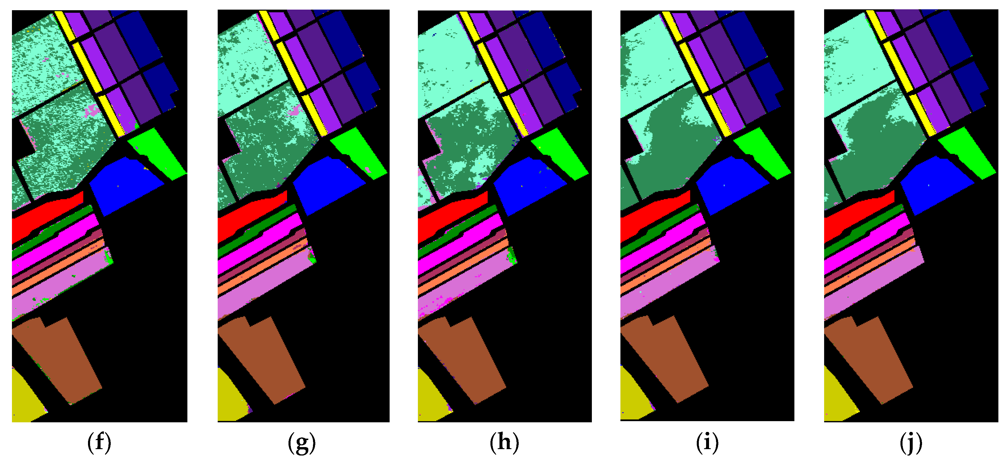
(3) The classification maps (shown in Figure 3 and Figure 4) and the analysis of adjustable parameters (shown in Figure 5) are also given for more details. We cannot guarantee that OAs obtained from SBLS with any parameter settings are the highest. This is mainly because, when there are too few nodes, much information is lost during the procedure of mapping.
Since there is no perfect thing, the drawbacks of the proposed SBLS method are summarized as follows:
(1) Similar to other types of classifiers, both BLS and SBLS are sensitive to input.
(2) If too many nodes in MF or EN are settled, much memory space will be used.
5. Conclusions
With advances of hyperspectral imaging techniques, HSI classification remains an active and challenging topic in the remote sensing community. Due to the difficulty of labeled samples, in this paper, a semi-supervised broad learning system-based HSI classification method called SBLS is proposed, which incorporates the class-probability into the broad learning. The designed model can take advantage of limited samples and large number of unlabeled samples simultaneously. Compared with deep learning-based methods, the weights of SBLS can be easily computed through ridge regression approximation instead of gradient descent methods. Nine classification methods including three traditional classifiers (SVM, ELM, and SPELM), one semi-supervised graph-based method (SSG), three deep learning-based methods (CNN-PPF, BASS-Net, and R-VCANet), one spectral-spatial method (HiFi-We), and the original broad learning system (BLS) are compared. Experimental results on three real hyperspectral datasets (Indian Pines, Salinas and Botswana) demonstrate that, under the condition of limited labeled samples, the proposed SBLS method can not only get higher classification accuracy, but also cost much less time than deep learning-based methods.
Moreover, the proposed SBLS still has space for further improvement. For instance, SBLS cannot determine the labels of samples when there is no a priori information. We will explore an unsupervised version of BLS for HSI clustering.
Author Contributions
All of the authors made significant contributions to the work. Y.K. and Y.C. conceived and designed the experiments; Y.K., X.W. and Y.C. performed the experiments; Y.K., X.W. and Y.C. analyzed the data; C.L.P.C. provided the codes about broad learning system; Y.K., X.W., Y.C., and C.L.P.C. wrote the paper.
Acknowledgments
This work was supported in part by the National Natural Science Foundation of China under Grant 61772532, Grant 61472424, and Grant 61703404.
Conflicts of Interest
The authors declare no conflict of interest.
References
- Gao, L.; Yang, B.; Du, Q.; Zhang, B. Adjusted spectral matched filter for target detection in hyperspectral imagery. Remote Sens. 2015, 7, 6611–6634. [Google Scholar] [CrossRef]
- Onoyama, H.; Ryu, C.; Suguri, M.; Lida, M. Integrate growing temperature to estimate the nitrogen content of rice plants at the heading stage using hyperspectral imagery. IEEE J. Sel. Top. Appl. Earth Obs. Remote Sens. 2014, 7, 2506–2515. [Google Scholar] [CrossRef]
- Brunet, D.; Sills, D. A generalized distance transform: Theory and applications to weather analysis and forecasting. IEEE Trans. Geosci. Remote Sens. 2017, 55, 1752–1764. [Google Scholar] [CrossRef]
- Islam, T.; Hulley, G.C.; Malakar, N.K.; Radocinski, R.G.; Guillevic, P.C.; Hook, S.J. A physics-based algorithm for the simultaneous retrieval of land surface temperature and emissivity from VIIRS thermal infrared data. IEEE Trans. Geosci. Remote Sens. 2017, 55, 563–576. [Google Scholar] [CrossRef]
- Li, W.; Du, Q.; Zhang, F.; Hu, W. Collaborative-representation-based nearest neighbor classifier for hyperspectral imagery. IEEE Geosci. Remote Sens. Lett. 2015, 12, 389–393. [Google Scholar] [CrossRef]
- Wu, Y.F.; Yang, X.H.; Plaza, A.; Qiao, F.; Gao, L.R.; Zhang, B.; Cui, Y.B. Approximate computing of remotely Sensed data: SVM hyperspectral image classification as a case study. IEEE J. Sel. Top. Appl. Earth Obs. Remote Sens. 2016, 9, 5806–5818. [Google Scholar] [CrossRef]
- Xue, Z.; Du, P.; Su, H. Harmonic analysis for hyperspectral image classification integrated with PSO optimized SVM. IEEE J. Sel. Top. Appl. Earth Obs. Remote Sens. 2014, 7, 2131–2146. [Google Scholar] [CrossRef]
- Li, W.; Chen, C.; Su, H.; Du, Q. Local binary patterns and extreme learning machine for hyperspectral imagery classification. IEEE Trans. Geosci. Remote Sens. 2015, 53, 3681–3693. [Google Scholar] [CrossRef]
- Alom, M.; Sidike, P.; Taha, T.; Asari, V. State preserving extreme learning machine: A monotonically increasing learning approach. Neural Process. Lett. 2016, 45, 703–725. [Google Scholar] [CrossRef]
- Feng, S.; Chen, C.L.P. A fuzzy restricted boltzmann machine: Novel learning algorithms based on crisp possibilistic mean value of fuzzy numbers. IEEE Trans. Fuzzy Syst. 2016. [Google Scholar] [CrossRef]
- Chen, C.L.P.; Zhang, C.Y.; Chen, L.; Gan, M. Fuzzy restricted boltzmann machine for the enhancement of deep learning. IEEE Trans. Fuzzy Syst. 2015, 23, 2163–2173. [Google Scholar] [CrossRef]
- Chen, Y.; Lin, Z.; Zhao, X.; Wang, G. Deep learning-based classification of hyperspectral data. IEEE J. Sel. Top. Appl. Earth Obs. Remote Sens. 2014, 7, 2094–2107. [Google Scholar] [CrossRef]
- Tao, C.; Pan, H.; Li, Y.; Zou, Z. Unsupervised spectral-spatial feature learning with stacked sparse autoencoder for hyperspectral imagery classification. IEEE Geosci. Remote Sens. Lett. 2015, 12, 2438–2442. [Google Scholar]
- Chen, Y.; Zhao, X.; Jia, X. Spectral-spatial classification of hyperspectral data based on deep belief network. IEEE J. Sel. Top. Appl. Earth Obs. Remote Sens. 2015, 8, 1–12. [Google Scholar] [CrossRef]
- Romero, A.; Gatta, C.; Camps-Valls, G. Unsupervised deep feature extraction for remote sensing image classification. IEEE Trans. Geosci. Remote Sens. 2016, 54, 1349–1362. [Google Scholar] [CrossRef]
- Li, W.; Wu, G.; Zhang, F.; Du, Q. Hyperspectral image classification using deep pixel-pair features. IEEE Trans. Geosci. Remote Sens. 2017, 55, 844–853. [Google Scholar] [CrossRef]
- Santara, A.; Mani, K.; Hatwar, P.; Singh, A.; Garg, A.; Padia, K.; Mitra, P. BASS net: Band-adaptive spectral-spatial feature learning neural network for hyperspectral image classification. IEEE Trans. Geosci. Remote Sens. 2017. [Google Scholar] [CrossRef]
- Pan, B.; Shi, Z.; Zhang, N.; Xie, S. Hyperspectral image classification based on nonlinear spectral-spatial network. IEEE Geosci. Remote Sens. Lett. 2016, 13, 1782–1786. [Google Scholar] [CrossRef]
- Pan, B.; Shi, Z.; Xu, X. R-VCANet: A new deep-learning-based hyperspectral image classification method. IEEE J. Sel. Top. Appl. Earth Obs. Remote Sens. 2017, 10, 1975–1986. [Google Scholar] [CrossRef]
- Chen, C.L.P.; Liu, Z. Broad learning system: An effective and efficient incremental learning system without the need for deep architecture. IEEE Trans. Neural Netw. Learn. Syst. 2017. [Google Scholar] [CrossRef] [PubMed]
- Chen, C.L.P.; Wan, J.Z. A rapid learning and dynamic stepwise updating algorithm for flat neural networks and the application to time-series prediction. IEEE Trans. Syst. Man Cybern. Part B 1999, 29, 62–72. [Google Scholar] [CrossRef] [PubMed]
- Chen, C.L.P. A rapid supervised learning neural network for function interpolation and approximation. IEEE Trans. Neural Netw. 1996, 7, 1220–1230. [Google Scholar] [CrossRef] [PubMed]
- Camps-Valls, G.; Marsheva, T.B.; Zhou, D. Semi-supervised graph-based hyperspectral image classification. IEEE Trans. Geosci. Remote Sens. 2007, 45, 3044–3054. [Google Scholar] [CrossRef]
- Belkin, M.; Niyogi, P.; Sindhwani, V. Manifold regularization: Ageometric framework for learning from examples. J. Mach. Learn. Res. 2006, 7, 2399–2434. [Google Scholar]
- Wang, F.; Zhang, C. Label propagation through linear neighborhoods. IEEE Trans. Knowl. Data Eng. 2008, 20, 55–67. [Google Scholar] [CrossRef]
- Zhuang, L.; Gao, S.; Tang, J.; Wang, J.; Lin, Z.; Ma, Y.; Yu, N. Constructing a nonnegative low-rank and sparse graph with data-adaptive features. IEEE Trans. Image Process. 2015, 24, 3717–3728. [Google Scholar] [CrossRef] [PubMed]
- De Morsier, F.; Borgeaud, M.; Gass, V.; Thiran, J.P.; Tuia, D. Kernel low-rank and sparse graph for unsupervised and semi-supervised classification of hyperspectral images. IEEE Trans. Geosci. Remote Sens. 2016, 54, 3410–3420. [Google Scholar] [CrossRef]
- Shao, Y.J.; Sang, N.; Gao, C.X.; Ma, L. Probabilistic class structure regularized sparse representation graph for semi-supervised hyperspectral image classification. Pattern Recognit. 2017, 63, 102–114. [Google Scholar] [CrossRef]
- Pan, B.; Shi, Z.W.; Xu, X. Hierarchical guidance filtering based ensemble classification for hyperspectral image. IEEE Trans. Geosci. Remote Sens. 2017, 55, 4177–4189. [Google Scholar] [CrossRef]
Figure 1.
Flowchart of HSI classification based on SBLS.

Figure 2.
Ground truth maps of three HSI datasets: (a) Indian Pines; (b) Salinas; and (c) Botswana.

Figure 3.
Classification maps on Indian pines dataset: (a) SVM; (b) ELM; (c) SPELM; (d) SSG; (e) CNN-PPF; (f) BASS-Net; (g) R-VCANet; (h) HiFi-We; (i) BLS; and (j) SBLS.
Figure 3.
Classification maps on Indian pines dataset: (a) SVM; (b) ELM; (c) SPELM; (d) SSG; (e) CNN-PPF; (f) BASS-Net; (g) R-VCANet; (h) HiFi-We; (i) BLS; and (j) SBLS.

Figure 4.
Classification maps on Salinas dataset: (a) SVM; (b) ELM; (c) SPELM; (d) SSG; (e) CNN-PPF; (f) BASS-Net; (g) R-VCANet; (h) HiFi-We; (i) BLS; and (j) SBLS.
Figure 4.
Classification maps on Salinas dataset: (a) SVM; (b) ELM; (c) SPELM; (d) SSG; (e) CNN-PPF; (f) BASS-Net; (g) R-VCANet; (h) HiFi-We; (i) BLS; and (j) SBLS.


Figure 5.
OA versus and : (a) Indian Pines; (b) Salinas; and (c) Botswana.


Table 1.
The proposed HSI classification method based on SBLS.
| Input: HGF-based HSI spectral-spatial representation. (a) Calculate class-probability matrix according to Equation (5). (b) Calculate pseudo labels for unlabeled samples according to Equation (6). (c) Calculate and according to Equations (7)–(8), respectively. (d) Calculate weights of BLS according to Equations (12)–(13). (e) Calculate predictive labels with Equations (7), (8), and (14), according to , , , , and . Output: predictive labels . |
Table 2.
Size of labeled and unlabeled samples for different HSI datasets.
| No. | Indian Pines | Salinas | Botswana | ||||||
|---|---|---|---|---|---|---|---|---|---|
| Surface Object | s.l.s. | s.u.s. | Surface Object | s.l.s. | s.u.s. | Surface Object | s.l.s. | s.u.s. | |
| 1 | Alfalfa | 20 | 26 | Brocoli_green_weeds_1 | 20 | 500 | Water | 20 | 250 |
| 2 | Corn-notill | 20 | 1408 | Brocoli_green_weeds_2 | 20 | 500 | Hippo grass | 20 | 81 |
| 3 | Corn-mintill | 20 | 810 | Fallow | 20 | 500 | Floodplain grasses1 | 20 | 231 |
| 4 | Corn | 20 | 217 | Fallow_rough_plow | 20 | 500 | Floodplain grasses2 | 20 | 195 |
| 5 | Grass-pasture | 20 | 463 | Fallow_smooth | 20 | 500 | Reeds1 | 20 | 249 |
| 6 | Grass-trees | 20 | 710 | Stubble | 20 | 500 | Riparian | 20 | 249 |
| 7 | Grass-pasture-mowed | 20 | 8 | Celery | 20 | 500 | Firescar2 | 20 | 239 |
| 8 | Hay-windrowed | 20 | 458 | Grapes_untrained | 20 | 500 | Island interior | 20 | 183 |
| 9 | Oats | 10 | 10 | Soil_vinyard_develop | 20 | 500 | Acacia woodlands | 20 | 294 |
| 10 | Soybean-notill | 20 | 952 | Corn_senesced_green_weeds | 20 | 500 | Acacia shrublands | 20 | 228 |
| 11 | Soybean-mintill | 20 | 2435 | Lettuce_romaine_4wk | 20 | 500 | Acacia grasslands | 20 | 285 |
| 12 | Soybean-clean | 20 | 573 | Lettuce_romaine_5wk | 20 | 500 | Short mopane | 20 | 161 |
| 13 | Wheat | 20 | 185 | Lettuce_romaine_6wk | 20 | 500 | Mixed mopane | 20 | 248 |
| 14 | Woods | 20 | 1245 | Lettuce_romaine_7wk | 20 | 500 | Exposed soils | 20 | 75 |
| 15 | Buildings-Grass-Trees-Drives | 20 | 366 | Vinyard_untrained | 20 | 500 | |||
| 16 | Stone-Steel-Towers | 20 | 73 | Vinyard_vertical_trellis | 20 | 500 | |||
Table 3.
Comparison of classification performance on Indian Pines dataset.
| Surface Object | SVM [6] | ELM [8] | SPELM [9] | SSG [23] | CNN-PPF [16] | BASS-Net [17] | R-VCANet [19] | HiFi-We [29] | BLS [20] | SBLS |
|---|---|---|---|---|---|---|---|---|---|---|
| Alfalfa (%) | 54.15 | 66.63 | 90.13 | 96.15 | 32.84 | 80.77 | 100 | 100 | 96.15 | 99.23 |
| Corn-notill (%) | 75.00 | 79.17 | 87.01 | 71.46 | 53.64 | 55.33 | 64.98 | 85.72 | 78.69 | 84.73 |
| Corn-mintill (%) | 72.11 | 87.93 | 85.30 | 84.07 | 56.36 | 59.75 | 86.05 | 91.36 | 98.52 | 94.49 |
| Corn (%) | 54.13 | 61.31 | 77.35 | 93.82 | 33.73 | 91.24 | 99.54 | 98.16 | 100 | 100 |
| Grass-pasture (%) | 87.88 | 98.58 | 94.31 | 85.40 | 79.34 | 89.42 | 91.14 | 91.14 | 96.33 | 90.67 |
| Grass-trees (%) | 98.15 | 99.40 | 99.62 | 97.35 | 94.67 | 94.93 | 99.30 | 99.86 | 90.14 | 99.86 |
| Grass-pasture-mowed (%) | 27.34 | 28.59 | 38.46 | 97.50 | 57.14 | 100 | 100 | 100 | 100 | 100 |
| Hay-windrowed (%) | 100 | 98.35 | 99.57 | 98.69 | 91.02 | 99.56 | 98.47 | 98.69 | 87.12 | 99.34 |
| Oats (%) | 66.21 | 73.78 | 94.85 | 100 | 58.82 | 100 | 100 | 100 | 100 | 100 |
| Soybean-notill (%) | 72.36 | 71.24 | 80.18 | 79.33 | 53.83 | 73.11 | 89.50 | 83.82 | 82.98 | 88.11 |
| Soybean-mintill (%) | 91.85 | 82.31 | 94.38 | 78.94 | 72.81 | 54.74 | 72.98 | 83.61 | 89.40 | 88.38 |
| Soybean-clean (%) | 75.78 | 57.59 | 82.56 | 78.25 | 43.46 | 63.18 | 95.64 | 87.09 | 97.91 | 93.40 |
| Wheat (%) | 99.78 | 99.47 | 100 | 99.14 | 98.90 | 98.92 | 98.92 | 99.46 | 100 | 99.68 |
| Woods (%) | 99.57 | 99.50 | 99.74 | 94.18 | 93.14 | 82.09 | 94.14 | 99.20 | 98.96 | 99.81 |
| Buildings-Grass-Trees-Drives (%) | 83.83 | 92.84 | 97.97 | 85.74 | 73.10 | 65.57 | 90.16 | 89.89 | 99.73 | 99.07 |
| Stone-Steel-Towers (%) | 99.19 | 96.35 | 98.12 | 98.63 | 87.18 | 98.63 | 100 | 98.63 | 98.63 | 99.18 |
| AA (%) | 78.58 | 80.82 | 88.72 | 89.91 | 67.50 | 81.70 | 92.55 | 94.16 | 94.66 | 95.99 |
| OA (%) | 83.56 | 83.01 | 90.78 | 83.91 | 67.20 | 69.95 | 84.36 | 89.94 | 90.88 | 92.47 |
| Kappa | 0.8139 | 0.8071 | 0.8950 | 0.8177 | 0.6325 | 0.6616 | 0.8234 | 0.8855 | 0.8959 | 0.9143 |
| t(s) | 0.98 | 0.34 | 35.80 | 372.96 | 1500.03 | 1251.78 | 3238.74 | 250.16 | 4.81 | 420.02 |
Table 4.
Comparison of classification performance on Salinas dataset.
| Surface Object | SVM [6] | ELM [8] | SPELM [9] | SSG [23] | CNN-PPF [16] | BASS-Net [17] | R-VCANet [19] | HiFi-We [29] | BLS [20] | SBLS |
|---|---|---|---|---|---|---|---|---|---|---|
| Brocoli_green_weeds_1 (%) | 100 | 100 | 100 | 98.06 | 99.95 | 99.50 | 99.60 | 99.66 | 99.97 | 100 |
| Brocoli_green_weeds_2 (%) | 99.80 | 100 | 99.95 | 93.84 | 98.84 | 99.65 | 99.87 | 99.19 | 99.51 | 99.81 |
| Fallow (%) | 91.07 | 99.80 | 99.88 | 88.20 | 78.47 | 99.49 | 98.06 | 99.06 | 100 | 99.96 |
| Fallow_rough_plow (%) | 97.33 | 97.01 | 98.87 | 94.29 | 95.81 | 98.84 | 98.91 | 99.07 | 99.33 | 99.80 |
| Fallow_smooth (%) | 97.26 | 91.77 | 96.82 | 90.32 | 96.21 | 97.03 | 99.32 | 98.59 | 98.98 | 99.13 |
| Stubble (%) | 99.70 | 99.97 | 99.98 | 94.54 | 99.61 | 99.80 | 98.65 | 99.20 | 99.78 | 99.80 |
| Celery (%) | 98.26 | 99.90 | 99.81 | 92.89 | 97.66 | 99.72 | 98.20 | 98.73 | 99.53 | 99.84 |
| Grapes_untrained (%) | 85.31 | 77.57 | 86.12 | 56.65 | 72.84 | 65.18 | 70.71 | 78.99 | 88.81 | 91.31 |
| Soil_vinyard_develop (%) | 99.20 | 98.43 | 98.50 | 89.73 | 99.08 | 98.61 | 99.74 | 99.87 | 99.97 | 99.65 |
| Corn_senesced_green_weeds (%) | 84.84 | 95.92 | 96.61 | 77.38 | 80.84 | 87.78 | 91.22 | 89.13 | 93.52 | 94.12 |
| Lettuce_romaine_4wk (%) | 86.68 | 92.56 | 96.49 | 89.43 | 63.20 | 92.18 | 98.66 | 97.73 | 99.54 | 99.79 |
| Lettuce_romaine_5wk (%) | 97.27 | 97.76 | 95.56 | 95.02 | 91.72 | 98.53 | 100 | 99.97 | 99.94 | 100 |
| Lettuce_romaine_6wk (%) | 96.52 | 88.63 | 96.41 | 91.58 | 96.84 | 96.21 | 99.44 | 96.58 | 99.11 | 99.00 |
| Lettuce_romaine_7wk (%) | 86.62 | 76.20 | 88.69 | 89.60 | 88.61 | 96.95 | 97.33 | 96.50 | 97.18 | 97.10 |
| Vinyard_untrained (%) | 67.10 | 81.56 | 79.71 | 72.97 | 60.14 | 67.43 | 74.66 | 87.14 | 82.75 | 89.27 |
| Vinyard_vertical_trellis (%) | 99.24 | 99.93 | 99.98 | 88.35 | 96.74 | 98.15 | 99.44 | 95.86 | 98.68 | 98.80 |
| AA (%) | 92.89 | 93.56 | 95.84 | 87.68 | 88.53 | 93.44 | 95.23 | 95.95 | 97.28 | 97.96 |
| OA (%) | 89.12 | 90.73 | 93.29 | 81.21 | 84.76 | 86.77 | 89.42 | 92.56 | 94.67 | 96.14 |
| Kappa | 0.8793 | 0.8965 | 0.9252 | 0.7927 | 0.8306 | 0.8533 | 0.8824 | 0.9174 | 0.9406 | 0.9570 |
| t(s) | 3.26 | 1.68 | 131.60 | 156.20 | 1560.19 | 1294.50 | 17,080.47 | 352.24 | 13.95 | 240.26 |
Table 5.
Comparison of classification performance on Botswana dataset.
| Surface Object | SVM [6] | ELM [8] | SPELM [9] | SSG [23] | CNN-PPF [16] | BASS-Net [17] | R-VCANet [19] | HiFi-We [29] | BLS [20] | SBLS |
|---|---|---|---|---|---|---|---|---|---|---|
| Water (%) | 100 | 99.84 | 100 | 100 | 99.21 | 100 | 100 | 100 | 100 | 98.32 |
| Hippo grass (%) | 88.89 | 93.33 | 97.83 | 87.90 | 100 | 100 | 100 | 96.05 | 99.26 | 97.28 |
| Floodplain grasses1 (%) | 95.43 | 98.5 | 99.57 | 98.35 | 100 | 99.57 | 100 | 96.62 | 100 | 100 |
| Floodplain grasses2 (%) | 91.26 | 78.09 | 95.81 | 96.21 | 94.20 | 97.44 | 100 | 99.49 | 99.28 | 100 |
| Reeds1 (%) | 89.19 | 94.79 | 93.8 | 79.52 | 89.02 | 86.35 | 96.79 | 90.84 | 93.57 | 96.87 |
| Riparian (%) | 62.43 | 100 | 100 | 77.83 | 78.74 | 82.33 | 90.36 | 94.46 | 87.71 | 99.28 |
| Firescar2 (%) | 97.07 | 100 | 100 | 98.74 | 94.35 | 100 | 100 | 95.73 | 100 | 100 |
| Island interior (%) | 97.83 | 98.19 | 98.71 | 97.27 | 87.56 | 100 | 100 | 100 | 100 | 100 |
| Acacia woodlands (%) | 93.40 | 87.69 | 98.47 | 93.47 | 92.09 | 94.22 | 87.07 | 95.78 | 99.25 | 99.86 |
| Acacia shrublands (%) | 75.18 | 88.31 | 99.39 | 90.61 | 93.62 | 96.49 | 99.56 | 98.77 | 100 | 100 |
| Acacia grasslands (%) | 93.85 | 99.02 | 99.93 | 88.14 | 95.40 | 92.63 | 97.54 | 94.95 | 100 | 100 |
| Short mopane (%) | 89.70 | 94.43 | 98.43 | 98.14 | 100 | 100 | 100 | 97.52 | 100 | 100 |
| Mixed mopane (%) | 89.52 | 97.80 | 99.84 | 92.42 | 95.38 | 95.56 | 99.19 | 93.79 | 98.47 | 99.27 |
| Exposed soils (%) | 94.94 | 99.84 | 100 | 97.87 | 100 | 100 | 98.67 | 99.73 | 98.93 | 97.33 |
| AA (%) | 96.51 | 94.61 | 98.70 | 92.61 | 94.26 | 96.04 | 97.80 | 96.70 | 98.32 | 99.16 |
| OA (%) | 96.71 | 94.16 | 98.67 | 92.15 | 93.40 | 95.25 | 97.27 | 96.36 | 98.13 | 99.32 |
| Kappa | 0.9644 | 0.9367 | 0.9856 | 0.9149 | 0.9284 | 0.9485 | 0.9704 | 0.9606 | 0.9798 | 0.9926 |
| t(s) | 1.59 | 1.31 | 12.57 | 16.35 | 1020.09 | 1120.53 | 908.54 | 439.56 | 3.83 | 70.97 |
© 2018 by the authors. Licensee MDPI, Basel, Switzerland. This article is an open access article distributed under the terms and conditions of the Creative Commons Attribution (CC BY) license (http://creativecommons.org/licenses/by/4.0/).
Share and Cite
MDPI and ACS Style
Kong, Y.; Wang, X.; Cheng, Y.; Chen, C.L.P. Hyperspectral Imagery Classification Based on Semi-Supervised Broad Learning System. Remote Sens. 2018, 10, 685. https://doi.org/10.3390/rs10050685
AMA Style
Kong Y, Wang X, Cheng Y, Chen CLP. Hyperspectral Imagery Classification Based on Semi-Supervised Broad Learning System. Remote Sensing. 2018; 10(5):685. https://doi.org/10.3390/rs10050685
Chicago/Turabian StyleKong, Yi, Xuesong Wang, Yuhu Cheng, and C. L. Philip Chen. 2018. "Hyperspectral Imagery Classification Based on Semi-Supervised Broad Learning System" Remote Sensing 10, no. 5: 685. https://doi.org/10.3390/rs10050685
Note that from the first issue of 2016, this journal uses article numbers instead of page numbers. See further details here.